DIFFERENTIAL EQUATIONS

AND

CONTROL PROCESSES

N. 4, 2020

Electronic Journal,
reg. N ${\Phi}$C77-39410 at 15.04.2010

ISSN 1817-2172

http://diffjournal.spbu.ru/

e-mail: jodiff@mail.ru

Numerical methods

A Numerical-Analytical Method for Constructing Periodic Solutions of the Lorenz System

Abstract. This article describes a method for constructing approximations to periodic solutions of dynamic Lorenz system with classical values of the system parameters. The author obtained a system of nonlinear algebraic equations in general form concerning of the cyclic frequency, constant terms and amplitudes of harmonics that make up harmonic approximations to the desired solutions. The initial approximation for the Newton method is selected, which converges to a solution describing a periodic solution different from the equilibrium position. The results of a computational experiment are presented. The results are verified using high-precision calculations.

Keywords: Attractor, Lorenz Attractor, Trigonometric Polynomial, Newton’s Method.

1 Introduction

Let us consider the nonlinear system of differential equations introduced by E. Lorenz in [1]

$$\left\{\begin{array}[]{l}\dot{x}_{1}=\sigma(x_{2}-x_{1}),\vskip 6.0pt plus 2.0pt minus 2.0pt\\ \dot{x}_{2}=rx_{1}-x_{2}-x_{1}x_{3},\vskip 6.0pt plus 2.0pt minus 2.0pt\\ \dot{x}_{3}=x_{1}x_{2}-bx_{3},\end{array}\right.$$ (1)

where $\sigma=10$, $r=28$ and $b=8/3$ are the classical values of the system parameters.

Let us denote by $X(t)=\left[x_{1}(t)\>\>x_{2}(t)\>\>x_{3}(t)\right]^{\scriptsize\mbox{T}}$. It is proved in the article [1] that there exists a number $C>0$ such that for any solution $X(t)$ of the system (1), starting at time moment, $|X(t)|<C$, and the divergence of the vector velocity field of the system (1) is negative everywhere in $\mathbb{R}^{3}$ for classical values of the system parameters. Then [1] there exists a limit set, called the Lorenz attractor, to which all trajectories of the dynamical system are attracted when time tends to infinity. Thus the attractor determines the behavior of the solutions of a dynamical system over large segments of time.

W. Tucker in his work [2] proved that the attractor is hyperbolic in the system (1), that is, the attractor consists of cycles everywhere dense on it along which the near trajectories diverge exponentially. This creates their chaotic behavior.

As know [3, 4], the symbolic dynamics is used to track cycles in the Lorenz system. The region in the phase space containing the attractor is divided into a finite number of subdomains. Denoting each partition element by a symbol, the trajectories on the attractor passing through the corresponding regions are encoded by sequences of such symbols. If the sequence has regularity (repeatability of groups of characters), then we have a cycle. However, the return of trajectories in a neighborhood of its part does not mean its closure. A critique of the results of such computational experiments can be found, for example, in [5].

In 2004, D. Viswanath published the paper [6], in which he presented the initial conditions and periods for three cycles in the Lorenz attractor with a high accuracy. The calculation algorithm is based on the Lindstedt-Poincaré (LP) method, which (unlike numerical integration methods) is not affected by the stability of the cycle to which approximations are constructed.

An analysis of the Viswanath’s articles [6, 7] showed that the author gives a general description of the algorithm without reference to the computer implementation (in MATLAB as indicated in his works). Moreover, it is not clear how the obtained inhomogeneous linear system of differential equations with periodic coefficients is symbolically solved by the LP-method. For example, this can be done for the Van der Pol equation without any special problems.

In the article [6] Viswanath showed data that can be verified by solving the Cauchy problem with high-precision numerical methods (for example, [8]), but the details of the algorithm are not disclosed.

Therefore, it is important here to obtain the values of the initial conditions and the period with a given accuracy, having described in detail the implementation of the cycles search algorithm in the system (1).

The goal of this article is to develop a numerical-analytical method for constructing approximations to periodic solutions of the Lorenz system, which is simpler to implement than the LP-method. In this case, a system of nonlinear algebraic equations concerning of the cyclic frequency, constant terms, and amplitudes of harmonics making up the desired solution will be obtained in general form.

2 A Numerical-Analytical Method

Attempts to construct approximate periodic solutions in the system (1) with were made before Viswanath (for example, [9]) by the method of harmonic balance, but with low accuracy in representing real numbers, while in the article [9] initial conditions and periods of found cycles are not indicated (only drawings with cycles are given). Now this method is actively developing in the works of [10, 11, 12] A. Luo to find periodic solutions of nonlinear systems of differential equations.

Next, we describe a numerical-analytical method for constructing approximations to periodic solutions of the system (1). We make for this an approximation of the phase coordinates on the period $T$ by trigonometric polynomials in general form with an unknown cyclic frequency $\omega$ (since we do not know the value of $T$; in the general case, it can be an irrational number):

$$\begin{array}[]{l}\displaystyle x_{1}(t)\approx\tilde{x}_{1}(t)=x_{1,0}+\sum_{i=1}^{h}\left(c_{1,i}\cos(i\omega t)+s_{1,i}\sin(i\omega t)\right),\vskip 6.0pt plus 2.0pt minus 2.0pt\\ \displaystyle x_{2}(t)\approx\tilde{x}_{2}(t)=x_{2,0}+\sum_{i=1}^{h}\left(c_{2,i}\cos(i\omega t)+s_{2,i}\sin(i\omega t)\right),\vskip 6.0pt plus 2.0pt minus 2.0pt\\ \displaystyle x_{3}(t)\approx\tilde{x}_{3}(t)=x_{3,0}+\sum_{i=1}^{h}\left(c_{3,i}\cos(i\omega t)+s_{3,i}\sin(i\omega t)\right),\end{array}$$

where $h$ is given number of harmonics. If $i>h$, then we assume

$$c_{1,i}=s_{1,i}=c_{2,i}=s_{2,i}=c_{3,i}=s_{3,i}=0.$$ (2)

By the right-hand side of the system (1), we compose the residuals

$$\begin{array}[]{l}\delta_{1}(t)=\tilde{x}^{\prime}_{1}(t)-\sigma[\tilde{x}_{2}(t)-\tilde{x}_{1}(t)],\\ \delta_{2}(t)=\tilde{x}^{\prime}_{2}(t)-[r\tilde{x}_{1}(t)-\tilde{x}_{2}(t)-\tilde{x}_{1}(t)\tilde{x}_{3}(t)],\\ \delta_{3}(t)=\tilde{x}^{\prime}_{3}(t)-[\tilde{x}_{1}(t)\tilde{x}_{2}(t)-b\tilde{x}_{3}(t)],\end{array}$$

where the prime denotes the time derivative of the function. If we make calculations in an analytical form, then for each residual you need the following:

1. Differentiate by time the corresponding trigonometric polynomial;

2. Where there are products of phase coordinates, multiply the corresponding trigonometric polynomials, converting the products of trigonometric functions into sums;

3. Give similar terms for each function $\cos()$ and $\sin()$ with the corresponding argument;

4. By virtue of the equalities (2), to cut off the higher-order harmonics from the resulting residual;

5. Set the resulting residual to zero, i.e., coefficients at its harmonics.

If we put together the found algebraic equations for each residual, we obtain a still unclosed system of nonlinear equations concerning of unknown amplitudes $c_{1,i}$, $s_{1,i}$, $c_{2,i}$, $s_{2,i}$, $c_{3,i}$ and $s_{3,i}$ ($i=\overline{1,h}$), constant terms $x_{1,0}$, $x_{2,0}$ and $x_{3,0}$ and the cyclic frequency $\omega$. The number of unknown variables in the system is $3(1+2h)+1=6h+4$, but the equations are one less.

An additional equation can be taken from the following considerations. It is known (see [4, 6]) that the desired cycles intersect the plane passing through the equilibrium positions of the system (1)

$$O_{1}\left(-\sqrt{b(r-1)},\,-\sqrt{b(r-1)},\,r-1\right),\>\>O_{2}\left(\sqrt{b(r-1)},\,\sqrt{b(r-1)},\,r-1\right)$$ (3)

and parallel to the plane $x_{1}Ox_{2}$ (a Poincare section). Then the third coordinate in the initial condition for the desired cycles is equal to $r-1$, whence $\tilde{x}_{3}(0)=r-1$.

Therefore the additional equation of the system has the form:

$$x_{3,0}+\sum_{i=1}^{h}c_{3,i}-27=0.$$

The author did not find in literature of other additional information on the periodic solutions in the Lorenz system. Note that for the three cycles found by Viswanath, in the initial condition for the third coordinate, the number 27 was taken.

Next, we give an example of a system of equations for $h=2$:

$$\left\{\begin{aligned} \omega s_{1,1}-10c_{2,1}+10c_{1,1}&=0,\\ -10s_{2,1}+10s_{1,1}-c_{1,1}\omega&=0,\\ 2\omega s_{1,2}-10c_{2,2}+10c_{1,2}&=0,\\ -10s_{2,2}+10s_{1,2}-2c_{1,2}\omega&=0,\\ 10x_{1,0}-10x_{2,0}&=0,\\ c_{1,1}x_{3,0}+c_{3,1}x_{1,0}+\dfrac{s_{1,1}s_{3,2}}{2}+\dfrac{s_{1,2}s_{3,1}}{2}+\omega s_{2,1}+\dfrac{c_{1,1}c_{3,2}}{2}+\dfrac{c_{1,2}c_{3,1}}{2}+c_{2,1}-28c_{1,1}&=0,\\ s_{1,1}x_{3,0}+s_{3,1}x_{1,0}+\dfrac{c_{1,1}s_{3,2}}{2}-\dfrac{c_{1,2}s_{3,1}}{2}+s_{2,1}+\dfrac{c_{3,1}s_{1,2}}{2}-\dfrac{c_{3,2}s_{1,1}}{2}-28s_{1,1}-c_{2,1}\omega&=0,\\ c_{1,2}x_{3,0}+c_{3,2}x_{1,0}-\dfrac{s_{1,1}s_{3,1}}{2}+2\omega s_{2,2}+\dfrac{c_{1,1}c_{3,1}}{2}+c_{2,2}-28c_{1,2}&=0,\\ s_{1,2}x_{3,0}+s_{3,2}x_{1,0}+\dfrac{c_{1,1}s_{3,1}}{2}+s_{2,2}-28s_{1,2}+\dfrac{c_{3,1}s_{1,1}}{2}-2c_{2,2}\omega&=0,\\ x_{1,0}x_{3,0}+x_{2,0}-28x_{1,0}+\dfrac{s_{1,2}s_{3,2}}{2}+\dfrac{s_{1,1}s_{3,1}}{2}+\dfrac{c_{1,2}c_{3,2}}{2}+\dfrac{c_{1,1}c_{3,1}}{2}&=0,\\ -c_{1,1}x_{2,0}-c_{2,1}x_{1,0}+\omega s_{3,1}-\dfrac{s_{1,1}s_{2,2}}{2}-\dfrac{s_{1,2}s_{2,1}}{2}+\dfrac{8c_{3,1}}{3}-\dfrac{c_{1,1}c_{2,2}}{2}-\dfrac{c_{1,2}c_{2,1}}{2}&=0,\\ -s_{1,1}x_{2,0}-s_{2,1}x_{1,0}+\dfrac{8s_{3,1}}{3}-\dfrac{c_{1,1}s_{2,2}}{2}+\dfrac{c_{1,2}s_{2,1}}{2}-\dfrac{c_{2,1}s_{1,2}}{2}+\dfrac{c_{2,2}s_{1,1}}{2}-c_{3,1}\omega&=0,\\ -c_{1,2}x_{2,0}-c_{2,2}x_{1,0}+2\omega s_{3,2}+\dfrac{s_{1,1}s_{2,1}}{2}+\dfrac{8c_{3,2}}{3}-\dfrac{c_{1,1}c_{2,1}}{2}&=0,\\ -s_{1,2}x_{2,0}-s_{2,2}x_{1,0}+\dfrac{8s_{3,2}}{3}-\dfrac{c_{1,1}s_{2,1}}{2}-\dfrac{c_{2,1}s_{1,1}}{2}-2c_{3,2}\omega&=0,\\ \dfrac{8x_{3,0}}{3}-x_{1,0}x_{2,0}-\dfrac{s_{1,2}s_{2,2}}{2}-\dfrac{s_{1,1}s_{2,1}}{2}-\dfrac{c_{1,2}c_{2,2}}{2}-\dfrac{c_{1,1}c_{2,1}}{2}&=0,\\ x_{3,0}+c_{3,1}+c_{3,2}-27&=0.\end{aligned}\right.$$

Note that for any $h$ a similar system has solutions

$$\begin{array}[]{c}\displaystyle x_{1,0}=x_{2,0}=\pm\sqrt{b(r-1)},\>x_{3,0}=r-1,\>c_{k,i}=0,\>s_{k,i}=0,\\ \omega\>\mbox{is any number},\>\,k=\overline{1,3},\>i=\overline{1,h},\end{array}$$

corresponding to the equilibrium positions (3).

Therefore the resulting nonlinear system of algebraic equations has a non-unique solution. To find its approximate solutions, we will use the Newton numerical method, whose a convergence to the desired solution (i.e., describing a periodic solution of the system (1) different from its the equilibrium positions) depends on the choice of the initial approximation.

3 The Symbolic Computations to Obtain the System of Algebraic Equations

Thus, to obtain an approximation to the periodic solution, we must obtain a nonlinear system concerning of unknown decomposition coefficients and frequencies. As shown in the previous section, even for two harmonics, the system has a bulky form. Therefore, we consider the algorithm for performing symbolic calculations to obtain it.

When developing software [13], the Maxima math package (a computer algebra system) was chosen. The program for obtaining the amplitudes and constant terms of the residuals for $h=2$ is presented below.

/* [wxMaxima batch file version 1] [ DO NOT EDIT BY HAND! ]*/
/* [wxMaxima: input   start ] */
display2d:false$
x1:x10+c1c1*cos(1*omega*t)+s1c1*sin(1*omega*t)+
c1c2*cos(2*omega*t)+s1c2*sin(2*omega*t)$
x2:x20+c2c1*cos(1*omega*t)+s2c1*sin(1*omega*t)+
c2c2*cos(2*omega*t)+s2c2*sin(2*omega*t)$
x3:x30+c3c1*cos(1*omega*t)+s3c1*sin(1*omega*t)+
c3c2*cos(2*omega*t)+s3c2*sin(2*omega*t)$
assume(omega > 0)$
delta1:trigreduce(diff(x1,t)-(10*(x2-x1)),t)$
delta2:trigreduce(diff(x2,t)-(28*x1-x2-x1*x3),t)$
delta3:trigreduce(diff(x3,t)-(x1*x2-8/3*x3),t)$
expand(diff(delta1,cos(1*omega*t)));
expand(diff(delta1,sin(1*omega*t)));
expand(diff(delta1,cos(2*omega*t)));
expand(diff(delta1,sin(2*omega*t)));
expand(integrate(delta1,t,0,2*%pi/omega)*omega/(2*%pi));
expand(diff(delta2,cos(1*omega*t)));
expand(diff(delta2,sin(1*omega*t)));
expand(diff(delta2,cos(2*omega*t)));
expand(diff(delta2,sin(2*omega*t)));
expand(integrate(delta2,t,0,2*%pi/omega)*omega/(2*%pi));
expand(diff(delta3,cos(1*omega*t)));
expand(diff(delta3,sin(1*omega*t)));
expand(diff(delta3,cos(2*omega*t)));
expand(diff(delta3,sin(2*omega*t)));
expand(integrate(delta3,t,0,2*%pi/omega)*omega/(2*%pi));
/* [wxMaxima: input   end   ] */

The expression display2d:false$ turns off multi-line drawing of fractions, degrees, etc. The sign $ allows to calculate the result of an expression, but not display it (instead of ;). The function trigreduce(expression,t) collapses all products of trigonometric functions concerning of the variable $t$ in a combination of sums. Differentiation of residuals according to harmonic functions is necessary to obtain the corresponding amplitudes. The function expand(expression) expands brackets (performs multiplication, exponentiation, leads similar terms).

To find the constant terms of the residuals, their integration over the period is applied, i.e. the constant term of the $k$-residual is

$$\dfrac{\displaystyle\omega\int_{0}^{\frac{2\pi}{\omega}}\delta_{k}(t)dt}{2\pi}.$$

So that during symbolic integration the package does not ask a question about the sign of the frequency, a command is given assume(omega > 0)$.

A file with package commands is generated similarly for any number of $h$ harmonics by a computer program written in C++ [13]. After executing this program, the package will output symbolic expressions to the console for the left side of the system of algebraic equations, which will be solved in it by the Newton method.

Note that the most time-consuming operation here is symbolic integration. For example, for 120 harmonics, the system formation time is more than 2 days. We can here parallelize the computational process on three computers, but this will not have a significant effect. Therefore, a system of algebraic equations must be formed immediately. Next, we get a general form of this system. Note that when solving the system of nonlinear equations by the Newton method, the Jacobi matrix for the left side of the system does not invert. The Maxima package uses LU decomposition to solve a system of linear equations at each iteration of the method.

4 General Form of the System of Algebraic Equations

Since the right-hand side of the (1) system contains nonlinearities in the form of products of phase coordinates, let us obtain relations expressing the coefficients of trigonometric polynomials obtained by multiplying the approximations $\tilde{x}_{1}(t)\tilde{x}_{3}(t)$ and $\tilde{x}_{1}(t)\tilde{x}_{2}(t)$.

We consider two functions $f(t)$ and $F(t)$ represented by Fourier series

$$\begin{array}[]{c}\displaystyle f(t)=a_{0}+\sum_{i=1}^{\infty}\left(a_{i}\cos(i\omega t)+b_{i}\sin(i\omega t)\right),\vskip 6.0pt plus 2.0pt minus 2.0pt\\ \displaystyle F(t)=A_{0}+\sum_{i=1}^{\infty}\left(A_{i}\cos(i\omega t)+B_{i}\sin(i\omega t)\right).\end{array}$$

Let

$$f(t)F(t)=\alpha_{0}+\sum_{i=1}^{\infty}\left(\alpha_{i}\cos(i\omega t)+\beta_{i}\sin(i\omega t)\right).$$

Following the book [14, pp. 123-125], we have the relations:

$$\alpha_{0}=a_{0}A_{0}+\dfrac{1}{2}\sum_{m=1}^{\infty}\left(a_{m}A_{m}+b_{m}B_{m}\right),$$

$$\alpha_{i}=a_{0}A_{i}+\dfrac{1}{2}\sum_{m=1}^{\infty}\left(a_{m}(A_{m+i}+A_{m-i})+b_{m}(B_{m+i}+B_{m-i})\right),$$ (4)

$$\beta_{i}=a_{0}B_{i}+\dfrac{1}{2}\sum_{m=1}^{\infty}\left(a_{m}(B_{m+i}-B_{m-i})-b_{m}(A_{m+i}-A_{m-i})\right).$$ (5)

We assume that for $i>h$

$$a_{i}=b_{i}=A_{i}=B_{i}=0.$$

Since for our problem we find for an approximation up to and including the $h$-harmonic, we zero all the amplitudes in the product for $i>h$, i.e.

$$\alpha_{i}=\beta_{i}=0.$$

Thus, we pass from the product of series to the product of trigonometric polynomials. Also in the relations (4) and (5) we will assume [14, p. 124] that

$$A_{m-i}=A_{i-m},\>\>B_{m-i}=-B_{i-m},\>\>B_{0}=0.$$

Then we get

$$\alpha_{0}=a_{0}A_{0}+\dfrac{1}{2}\sum_{m=1}^{h}\left(a_{m}A_{m}+b_{m}B_{m}\right),$$

$$\alpha_{i} =a_{0}A_{i}+\dfrac{1}{2}\sum_{m=1}^{\infty}a_{m}A_{m+i}+\dfrac{1}{2}\sum_{m=1}^{\infty}a_{m}A_{m-i}+\dfrac{1}{2}\sum_{m=1}^{\infty}b_{m}B_{m+i}+\dfrac{1}{2}\sum_{m=1}^{\infty}b_{m}B_{m-i}=$$

$$=a_{0}A_{i}+\dfrac{1}{2}\sum_{m=1}^{h-i}a_{m}A_{m+i}+\dfrac{1}{2}a_{i}A_{0}+\dfrac{1}{2}\sum_{m=1}^{i-1}a_{m}A_{i-m}+\dfrac{1}{2}\sum_{m=i+1}^{h}a_{m}A_{m-i}+$$

$$+\dfrac{1}{2}\sum_{m=1}^{h}b_{m}B_{m+i}+\dfrac{1}{2}b_{i}B_{0}-\dfrac{1}{2}\sum_{m=1}^{i-1}b_{m}B_{i-m}+\dfrac{1}{2}\sum_{m=i+1}^{h}b_{m}B_{m-i}=$$

$$=a_{0}A_{i}+a_{i}A_{0}+\dfrac{1}{2}\sum_{m=1}^{h-i}\left(a_{m}A_{m+i}+b_{m}B_{m+i}\right)+\dfrac{1}{2}\sum_{m=1}^{i-1}\left(a_{m}A_{i-m}-b_{m}B_{i-m}\right)+$$

$$+\dfrac{1}{2}\sum_{m=i+1}^{h}\left(a_{m}A_{m-i}+b_{m}B_{m-i}\right),$$

$$\beta_{i} =a_{0}B_{i}+\dfrac{1}{2}\sum_{m=1}^{\infty}a_{m}B_{m+i}-\dfrac{1}{2}\sum_{m=1}^{\infty}a_{m}B_{m-i}-\dfrac{1}{2}\sum_{m=1}^{\infty}b_{m}A_{m+i}+\dfrac{1}{2}\sum_{m=1}^{\infty}b_{m}A_{m-i}=$$

$$=a_{0}B_{i}+\dfrac{1}{2}\sum_{m=1}^{h-i}a_{m}B_{m+i}+\dfrac{1}{2}\sum_{m=1}^{i-1}a_{m}B_{i-m}-\dfrac{1}{2}\sum_{m=i+1}^{h}a_{m}B_{m-i}-$$

$$-\dfrac{1}{2}\sum_{m=1}^{h-i}b_{m}A_{m+i}+b_{i}A_{0}+\dfrac{1}{2}\sum_{m=1}^{i-1}b_{m}A_{i-m}+\dfrac{1}{2}\sum_{m=i+1}^{h}b_{m}A_{m-i}=$$

$$=a_{0}B_{i}+b_{i}A_{0}+\dfrac{1}{2}\sum_{m=1}^{h-i}\left(a_{m}B_{m+i}-b_{m}A_{m+i}\right)+\dfrac{1}{2}\sum_{m=1}^{i-1}\left(a_{m}B_{i-m}+b_{m}A_{i-m}\right)+$$

$$+\dfrac{1}{2}\sum_{m=i+1}^{h}\left(-a_{m}B_{m-i}+b_{m}A_{m-i}\right).$$

Applying the obtained formulas to calculate the products of trigonometric polynomials to the residuals, we can write the equations for the $i$-th harmonics ($i=\overline{1,h}$ is the number of harmonics, $k=\overline{1,3}$ is residual number):

$k=1$:

$$\begin{array}[]{r}i\omega s_{1,i}-10c_{2,i}+10c_{1,i}=0,\vskip 6.0pt plus 2.0pt minus 2.0pt\\ -i\omega c_{1,i}-10s_{2,i}+10s_{1,i}=0,\end{array}$$

the equation corresponding to the constant term for the first residual is

$$x_{1,0}-x_{2,0}=0,$$

$k=2$:

$$i\omega s_{2,i}-28c_{1,i}+c_{2,i}+x_{1,0}c_{3,i}+c_{1,i}x_{3,0} +\dfrac{1}{2}\sum_{m=1}^{h-i}\left(c_{1,m}c_{3,m+i}+s_{1,m}s_{3,m+i}\right)+$$

$$+\dfrac{1}{2}\sum_{m=1}^{i-1}\left(c_{1,m}c_{3,i-m}-s_{1,m}s_{3,i-m}\right)+$$

$$+\dfrac{1}{2}\sum_{m=i+1}^{h}\left(c_{1,m}c_{3,m-i}+s_{1,m}s_{3,m-i}\right)=0,$$

$$-i\omega c_{2,i}-28s_{1,i}+s_{2,i}+x_{1,0}s_{3,i}+s_{1,i}x_{3,0} +\dfrac{1}{2}\sum_{m=1}^{h-i}\left(c_{1,m}s_{3,m+i}-s_{1,m}c_{3,m+i}\right)+$$

$$+\dfrac{1}{2}\sum_{m=1}^{i-1}\left(c_{1,m}s_{3,i-m}+s_{1,m}c_{3,i-m}\right)+$$

$$+\dfrac{1}{2}\sum_{m=i+1}^{h}\left(-c_{1,m}s_{3,m-i}+s_{1,m}c_{3,m-i}\right)=0,$$

the equation corresponding to the constant term for the second residual is

$$-28x_{1,0}+x_{2,0}+x_{1,0}x_{3,0}+\dfrac{1}{2}\sum_{m=1}^{h}\left(c_{1,m}c_{3,m}+s_{1,m}s_{3,m}\right)=0,$$

$k=3$:

$$i\omega s_{3,i}-x_{1,0}c_{2,i}-c_{1,i}x_{2,0} -\dfrac{1}{2}\sum_{m=1}^{h-i}\left(c_{1,m}c_{2,m+i}+s_{1,m}s_{2,m+i}\right)-$$

$$-\dfrac{1}{2}\sum_{m=1}^{i-1}\left(c_{1,m}c_{2,i-m}-s_{1,m}s_{2,i-m}\right)-$$

$$-\dfrac{1}{2}\sum_{m=i+1}^{h}\left(c_{1,m}c_{2,m-i}+s_{1,m}s_{2,m-i}\right)+\dfrac{8}{3}c_{3,i}=0,$$

$$-i\omega c_{3,i}-x_{1,0}s_{2,i}-s_{1,i}x_{2,0} -\dfrac{1}{2}\sum_{m=1}^{h-i}\left(c_{1,m}s_{2,m+i}-s_{1,m}c_{2,m+i}\right)-$$

$$-\dfrac{1}{2}\sum_{m=1}^{i-1}\left(c_{1,m}s_{2,i-m}+s_{1,m}c_{2,i-m}\right)-$$

$$-\dfrac{1}{2}\sum_{m=i+1}^{h}\left(-c_{1,m}s_{2,m-i}+s_{1,m}c_{2,m-i}\right)+\dfrac{8}{3}s_{3,i}=0,$$

the equation corresponding to the constant term for the third residual is

$$-x_{1,0}x_{2,0}-\dfrac{1}{2}\sum_{m=1}^{h}\left(c_{1,m}c_{2,m}+s_{1,m}s_{2,m}\right)+\dfrac{8}{3}x_{3,0}=0,$$

the additional system equation is

$$x_{3,0}+\sum_{i=1}^{h}c_{3,i}-27=0.$$

5 The Results of the Computational Experiment

As a result of numerous computational experiments, the initial approximation was chosen for the cyclic frequency, constant terms, and amplitudes at $h=h_{1}=5$:

$$\begin{array}[]{c}\omega=4,\>\>x_{1,0}=x_{2,0}=x_{3,0}=0,\>\>c_{1,i}=-1,\>i=\overline{1,5},\\ s_{1,j}=0,\>j=1,3,4,5,\>\>s_{1,2}=1.\end{array}$$

This result is remarkable in that the Newton method converges to a solution different from the equilibrium positions. Therefore, to improve the accuracy of the approximate periodic solution, we consider a system of algebraic equations for the value of $h$ equal to some $h_{2}>h_{1}$.

The obtained numerical solution of the system for $h=h_{1}$ is taken as the initial approximation for amplitudes with indices $i\leq h_{1}$ for a system with $h=h_{2}$, and the values of the initial approximation for amplitudes with indices $i>h_{1}$ are assumed to be zero.

Table 1: The amplitudes of harmonics for $\tilde{x}_{1}(t)$, $x_{1,0}=0$.

$i$	$c_{1,i}$	$s_{1,i}$
1	$-5.780478259196228$	$8.56017654325353$
2	0	0
3	$3.160762628380509$	$2.239212141102876$
4	0	0
5	$0.6958870387616096$	$-0.7979388979225431$
6	0	0
7	$-0.1891992374027477$	$-0.1864921358925765$
8	0	0
9	$-0.04770429623010056$	$0.04554044367245914$
10	0	0
11	$0.01112322884679491$	$0.01209138588669679$
12	0	0
13	$0.003061207095371694$	$-0.002735092350544739$
14	0	0
15	$-6.744578887916229\cdot 10^{-4}$	$-7.748319471034087\cdot 10^{-4}$
16	0	0
17	$-1.960718247379475\cdot 10^{-4}$	$1.665584161919807\cdot 10^{-4}$
18	0	0
19	$4.116738805347028\cdot 10^{-5}$	$4.960493476144467\cdot 10^{-5}$
20	0	0
21	$1.254757391175977\cdot 10^{-5}$	$-1.018054283421179\cdot 10^{-5}$
22	0	0
23	$-2.518375902000733\cdot 10^{-6}$	$-3.173486439630506\cdot 10^{-6}$
24	0	0
25	$-8.025338211960923\cdot 10^{-7}$	$6.230623750431923\cdot 10^{-7}$
26	0	0
27	$1.541534734542893\cdot 10^{-7}$	$2.0292802821633\cdot 10^{-7}$
28	0	0
29	$5.130649139299358\cdot 10^{-8}$	$-3.813725452268523\cdot 10^{-8}$
30	0	0
31	$-9.43393531993558\cdot 10^{-9}$	$-1.297038481588497\cdot 10^{-8}$
32	0	0
33	$-3.278552746800046\cdot 10^{-9}$	$2.333260259021725\cdot 10^{-9}$
34	0	0
35	$5.76957885768651\cdot 10^{-10}$	$8.28626640138045\cdot 10^{-10}$

Table 2: The amplitudes of harmonics for $\tilde{x}_{2}(t)$, $x_{2,0}=0$.

$i$	$c_{2,i}$	$s_{2,i}$
1	$-2.32972926505593$	$10.89038310357172$
2	0	0
3	$5.86875317198698$	$-1.5832552129833$
4	0	0
5	$-0.9124249133801483$	$-2.200556873678218$
6	0	0
7	$-0.7154457265566421$	$0.3473932955614448$
8	0	0
9	$0.1175186702136983$	$0.2186139734768588$
10	0	0
11	$0.06473984670858603$	$-0.03723215039412078$
12	0	0
13	$-0.01127208646321726$	$-0.01877739524860192$
14	0	0
15	$-0.005359671824365359$	$0.003303445299126894$
16	0	0
17	$9.453499475830811\cdot 10^{-4}$	$0.001510235036151227$
18	0	0
19	$4.211022386354685\cdot 10^{-4}$	$-2.657049331814368\cdot 10^{-4}$
20	0	0
21	$-7.363528144366622\cdot 10^{-5}$	$-1.164013765469982\cdot 10^{-4}$
22	0	0
23	$-3.19419300699788\cdot 10^{-5}$	$2.017609175377016\cdot 10^{-5}$
24	0	0
25	$5.47663534401654\cdot 10^{-6}$	$8.710929378319451\cdot 10^{-6}$
26	0	0
27	$2.362852034076972\cdot 10^{-6}$	$-1.474901091428546\cdot 10^{-6}$
28	0	0
29	$-3.94532524722541\cdot 10^{-7}$	$-6.379296603810031\cdot 10^{-7}$
30	0	0
31	$-1.715198229248314\cdot 10^{-7}$	$1.049218598356554\cdot 10^{-7}$
32	0	0
33	$2.776045093375681\cdot 10^{-8}$	$4.59473450493284\cdot 10^{-8}$
34	0	0
35	$1.22681173575872\cdot 10^{-8}$	$-7.31171826830086\cdot 10^{-9}$

Table 3: The amplitudes of harmonics for $\tilde{x}_{3}(t)$, $x_{3,0}=23.04210397942006$.

$i$	$c_{3,i}$	$s_{3,i}$
1	0	0
2	$7.568410271550653$	$-9.50386584559212$
3	0	0
4	$-3.555327211552558$	$-1.844710563805469$
5	0	0
6	$-0.4741220131932616$	$1.279043179069961$
7	0	0
8	$0.4227292179138024$	$0.1274574086305204$
9	0	0
10	$0.03498415351761577$	$-0.1315337800809524$
11	0	0
12	$-0.03934013541135439$	$-0.009645786231708874$
13	0	0
14	$-0.002660052258813564$	$0.01145537653603837$
15	0	0
16	$0.003271688724557337$	$7.33752523103949\cdot 10^{-4}$
17	0	0
18	$2.024982256871223\cdot 10^{-4}$	$-9.206266886554897\cdot 10^{-4}$
19	0	0
20	$-2.560063570343799\cdot 10^{-4}$	$-5.58964460662525\cdot 10^{-5}$
21	0	0
22	$-1.542436654918173\cdot 10^{-5}$	$7.050327849098175\cdot 10^{-5}$
23	0	0
24	$1.926014222030195\cdot 10^{-5}$	$4.25261452471065\cdot 10^{-6}$
25	0	0
26	$1.170939944189529\cdot 10^{-6}$	$-5.225643926851625\cdot 10^{-6}$
27	0	0
28	$-1.409525591131397\cdot 10^{-6}$	$-3.21879984959824\cdot 10^{-7}$
29	0	0
30	$-8.83134288999026\cdot 10^{-8}$	$3.782652721710986\cdot 10^{-7}$
31	0	0
32	$1.010610960272394\cdot 10^{-7}$	$2.418021923473667\cdot 10^{-8}$
33	0	0
34	$6.606163280924149\cdot 10^{-9}$	$-2.689431432873997\cdot 10^{-8}$
35	0	0

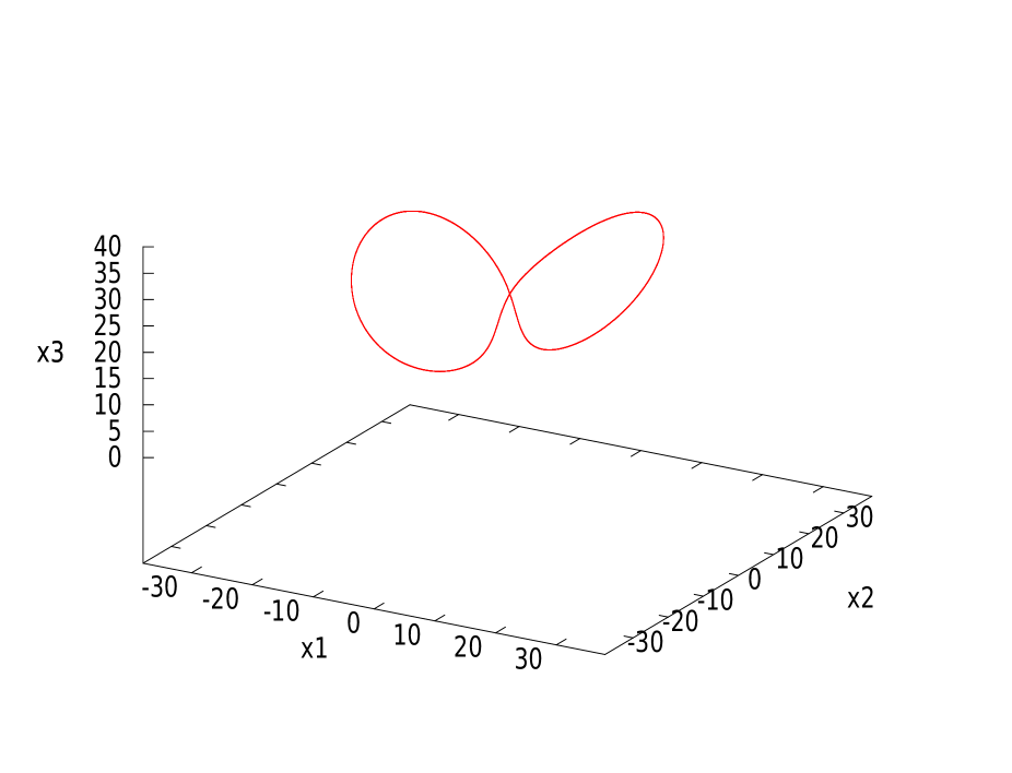
Figure 1: The cycle obtained by described method.

Tables 1–3 show the result of solving the system for $h=35$; the accuracy of the Newton method is $10^{-8}$. The period value is obtained equal to $T=1.558652210$, the initial condition for the obtained approximate periodic solution is

$$\begin{array}[]{c}\tilde{x}_{1}(0)=-2.147367631,\>\>\tilde{x}_{2}(0)=2.078048211,\>\>\tilde{x}_{3}(0)=27.\end{array}$$ (6)

The initial values (6) were checked on the period in a computer program that implements the numerical integration of the system (1) by the modified power series method [8] with an accuracy of estimating the common term of the series $10^{-25}$, 100 bits for mantissa real number and machine epsilon $1.57772\cdot 10^{-30}$. With such parameters of the method, the approximate values of the phase coordinates obtained by numerical integration were also verified by the same numerical method, but in reverse time. The values in the reverse time coincide with (6) up to the 9th character inclusive after the point. The resulting values of $x_{1}(T)$, $x_{2}(T)$ and $x_{3}(T)$ coincide with (6) up to the 8th character inclusive.

The cycle corresponding to (6) is shown in Fig. 1. Note that the cycle found coincides with the first Viswanath cycle in [6], all signs after the point for $T$ also coincide with the data from [6].

6 Acknowledgements

The reported study was funded by RFBR according to the research project 20-01-00347.

References

- [1] Lorenz, E. N. Deterministic Nonperiodic Flow, Journal of the Atmospheric Sciences, vol. 20, no. 2 (1963), pp. 130-141.
- [2] Tucker, W. A Rigorous ODE Solver and Smale’s 14th Problem, Foundations of Computational Mathematics, vol. 2, no. 1 (2002), pp. 53-117.
- [3] Rabinovich, M. I. Stochastic Self-Oscillations and Turbulence, Soviet Physics Uspekhi, vol. 21, no. 5 (1978), pp. 443-469.
- [4] Galias, Z., Tucker, W. Validated Study of the Existence of Short Cycles for Chaotic Systems Using Symbolic Dynamics and Interval Tools, International Journal of Bifurcation and Chaos, vol. 21, no. 2 (2011), pp. 551-563.
- [5] Lozi, R. Can We Trust in Numerical Computations of Chaotic Solutions of Dynamical Systems?, Topology and Dynamics of Chaos. In Celebration of Robert Gilmore’s 70th Birthday. - World Scientific Series in Nonlinear Science Series A, vol. 84 (2013), pp. 63-98.
- [6] Viswanath, D. The Fractal Property of the Lorenz Attractor, Physica D: Nonlinear Phenomena, vol. 190, no. 1-2 (2004), pp. 115-128.
- [7] Viswanath, D. The Lindstedt-Poincare Technique as an Algorithm for Computing Periodic Orbits, SIAM Review, vol. 43, no. 3 (2001), pp. 478-495.
- [8] Pchelintsev, A. N. Numerical and Physical Modeling of the Dynamics of the Lorenz System, Numerical Analysis and Applications, vol. 7, no. 2 (2014), pp. 159-167.
- [9] Neymeyr, K., Seelig, F. Determination of Unstable Limit Cycles in Chaotic Systems by Method of Unrestricted Harmonic Balance, Zeitschrift für Naturforschung A, vol. 46, no. 6 (1991), pp. 499-502.
- [10] Luo, A. C. J., Huang, J. Approximate Solutions of Periodic Motions in Nonlinear Systems via a Generalized Harmonic Balance, Journal of Vibration and Control, vol. 18, no. 11 (2011), pp. 1661-1674.
- [11] Luo, A. C. J. Toward Analytical Chaos in Nonlinear Systems, John Wiley & Sons, Chichester, ISBN: 978-1-118-65861-1, 2014, 258 pp.
- [12] Luo, A. C. J., Guo, S. Analytical Solutions of Period-1 to Period-2 Motions in a Periodically Diffused Brusselator, Journal of Computational and Nonlinear Dynamics, vol. 13, no. 9, 090912 (2018), 8 pp.
- [13] Pchelintsev, A. N. The Programs for Finding of Periodic Solutions in the Lorenz Attractor, GitHub, https://github.com/alpchelintsev/periodic_sols
- [14] Tolstov, G. P. Fourier Series, Dover Publications, New York (1962), 336 pp.