Fast Discovery of Heterogeneous Subsequences for Fast Trajectory Classification

Keywords Data Mining  $\cdot$ Multiple Aspect Trajectories  $\cdot$ Hiper Movelets  $\cdot$ Trajectory Classification, Sequence Classification

1 Introduction

Trajectory classification can be defined as the technique of discovering the class label of a moving object based on its trajectories [1]. It is important for several application domains as, for instance, identifying the transportation mode of a moving object [2], the strength level of a hurricane [1], a vessel type (cargo, fish, tourism, etc) [1], the owner user of a trajectory [3], etc.

A recent method for trajectory classification is MASTERMovelets, developed specifically for multiple aspect trajectories [3]. This method extracts movelets, which are subtrajectories that better discriminate each class, and are used as input to traditional classifiers. MASTERMovelets automatically explores all possible subtrajectories (or subsequences) of any size (e.g. one point, two points, three points, etc.) and explores all dimension combinations (e.g. space; space and time; space, time and POI category, etc), while seeking the best ones to represent the classes. The method Movelets[4] outperformed all previous works on raw trajectory classification.

The movelets are in general subtrajectories that are frequent in trajectories of one class and infrequent in trajectories of other classes, representing a certain behavior, or a routine. The quality of a movelet is computed based on the distance of a subtrajectory, called movelet candidate, to all subtrajectories of the same size (same number of points) in every class of the database. In real datasets, the combinatorial explosion of MASTERMovelets makes it very time consuming, but it outperformed all previous methods for trajectory classification in terms of accuracy.

The MASTERMovelets generates subtrajectories of all sizes (e.g. one point, two points, three points, etc) and dimension combinations, seeking for the best movelet candidates, meaning that for each subtrajectory there is an explosion of dimension combinations. This means that in a trajectory with ten points and three dimensions, will be generated $55$ subtrajectories, that with $7$ possible dimension combinations will result in $385$ movelet candidates. The problem is that with increasing dimensionality these numbers exponentially grow as, for instance, a trajectory with $20$ points and $6$ dimensions will result in $210$ subtrajectories, and $13,230$ movelet candidates. It will try $63$ dimension combinations for each subtrajectory, as the number of combinations is given by $2^{l}-1$, where $l$ is the number of dimensions. However, MASTERMovelets-Log can limit subtrajectories to the natural logarithm of its size. In the example, the trajectory with $20$ points and $6$ dimensions, MASTERMovelets-Log reduces to $74$ subtrajectories and $4,662$ movelet candidates. Although this strategy significantly reduces the computational cost, it still computes the distances of each subtrajectory to all subtrajectories of the entire dataset for comparisons, and generates a large number of movelets to use as input to classifiers, resulting in the curse of dimensionality problem.

Considering the MASTERMovelets high computational cost, in this work we propose a new method for discovering the movelets. We claim that frequent subtrajectories in a class will discriminate classes, as human behaviors commonly display recurrent movement patterns, which are more frequent for an object and less frequent for others.

2 Related Works

The algorithms Movelets [4] and MASTERMovelets [3] discover relevant subtrajectories, called movelets, without the need of extracting other features. The MASTERMovelets achieves a much better accuracy than Movelets. While Movelets encapsulates the distances of all trajectory dimensions in a single distance value, the MASTERMovelets keep distances in a vector using all data dimensions with the best combination. Ferrero et al. (2020) [3] also proposed MASTERMovelets-Log, which reduces the running time of the MASTERMovelets by limiting the size of the movelet candidates to the natural logarithm of the trajectory size. However, the processing time and computational cost are still extremely high. MASTERMovelets [3] was developed for multiple aspect trajectory classification, specifically, and largely outperformed state of the art methods in terms of accuracy. Moreover, the movelets are interpretable results, giving insights about the data. It is important for researchers looking for vaccines, for instance, that the classification results can be explainable and understandable.

The work of [5] can perform much faster than Movelets [4], with similar classification accuracy for a single dimension. To use several dimensions, the user must manually test and select the best dimensions combination. While, MASTERMovelets automatically selects the best dimension combinations with heterogeneous and different numbers of dimensions to generate movelets.

MARC, proposed by [6], is a recent work that uses word embeddings [7]. It encapsulates all trajectory dimensions: space, time and semantics, and use them as input to a neural network classifier. It is the first work to use the geoHash [8] on the spatial dimension, combined with other dimensions. MARC outperforms the Movelets [4] with very high accuracy when using all dimensions, as Movelets is unable to choose the best dimensions. However, the resulting patterns of MARC are not interpretable, as the classifier is limited to neural networks.

Some works for trajectory classification were developed for solving a single problem, as transportation mode inference [2, 9, 10], while the works of [11, 4, 6, 3] were developed for general purposes, such as level of hurricane, animal types, transportation modes, trajectory users, etc.

Since Movelets and MASTERMovelets are inspired by shapelets, we included works in time series optimization. Several optimizations are used in these works, as for instance, early abandoning [12, 13], SAX to reduction of search space and run time [14], and sampling the dataset for fast candidate search [15]. The early abandoning technique is not useful for movelets because multiple aspect trajectories are in general more sparse than time series, and this technique is interesting for sequences with high number of points.

Other works used statistical analysis, such as an Analysis of Variance A(NOVA) metric employed by Zuo et. al. [16]. In time series numerical values, statistical analysis can be used to identify regions from which to extract shapelets that have discriminant power over other classes. It is also used to filter redundant and low-quality candidates. Another work, proposed by Zhang et. al. [17], used Local Fisher Discriminant Analysis (LFDA) to determine the most relevant parts of the time series from which to extract shapelet candidates that are most likely to achieve good results. The works in time series, as the above mentioned, generally search discriminant shapelets in one dimension individually, while MASTERMovelets evaluates the dimensions individually and combined with others.

3 HiPerMovelets: A method for High Performance Movelet Extraction

In this section we propose a new method for reducing the search space for finding movelets, called HiPerMovelets. The method is inspired by the greedy search algorithm for feature selection proposed in [18], as an optimization for MASTERMovelets [3]. Our method is class-aware, and deals with one class at a time instead of all the classes in the dataset at once, thus reducing the search space and time for finding the movelets.

3.1 Main Definitions

Movelet candidates in [3] represent subtrajectories with different sizes and any dimension combination. As we propose to reduce the search space for movelets discovery, we define a different type of movelet candidate, described in Definition 1. In our method, a movelet candidate is a subtrajectory that is frequent in the trajectories of a class.

Definition 1.

Movelet Candidate. A movelet candidate is a tuple $\mathcal{M}=(T_{i},s_{(start,end)},C,\mathbb{W},L,\textbf{T}^{c})$, where $T_{i}$ is a trajectory from T’; $s_{start,end}$ is a subtrajectory extracted from $T_{i}$; $C$ is a subset with the candidate dimensions, and $C\subseteq D$; $\mathbb{W}$ is a set of pairs $(W^{s}_{T_{j}},class_{T_{j}})$, where $W^{s}_{T_{j}}$ is a distance vector that contains the distances of the best alignment of $\mathcal{M}$ to every trajectory T’, the same class as ${T_{j}}$. The distances are calculated using the best alignment between $s_{(start,end)}$ and each trajectory ${T_{j}}$ in the dimensions $C$; $\textbf{T}^{c}$ are the covered trajectories, i.e., a subset of class trajectories that contain the candidate $\mathcal{M}$ ($\textbf{T}^{c}\subseteq\textbf{T'}$); $L$ is a pair $(sp,quality)$, where $sp$ is a set of distances $W^{s}_{T_{j}}$, with one value for each dimension, that better divide the classes (used to measure the candidate relevance), and quality is a relative frequency score given to the candidate $\mathcal{M}$.

The quality score of a movelet candidate is based on the relative frequency (a proportion) that it appears in its class trajectories. For each dimension of a movelet candidate, we define a relative frequency as presented in Equation 1. It describes the relative frequency function for a dimension $k$ ($freq_{k}$) from a movelet candidate $\mathcal{M}_{j}$ to the trajectories T’ of a class:

$$freq_{k}=\frac{\sum^{i=|\textbf{T'}|}_{i=1}\left(max({W^{*}[k]})-W^{s}_{T_{i}}[k]\right)}{max({W^{*}[k]}).|\textbf{T'}|}$$ (1)

Where $W^{*}$ is a multidimensional vector of trajectory distances from extracted candidates to trajectories of the class (T’), and $W^{s}_{T_{i}}[k]$ is the distance value from the movelet candidate to the trajectory $T_{i}\in\textbf{T'}$ in the dimension $k\in C$. To make the proportion more accurate, we normalize the distance value by subtracting it from the maximum distance value ($max({W^{*}[k]})$) in that dimension. The frequency is the average between the sum of the distances and the maximum possible sum of distances ($max({W^{*}[k]}).|\textbf{T'}|$). The quality of a movelet candidate (Equation 2) is the average proportion that a candidate has in trajectories T’ of its class in each dimension $k$.

$$\textit{Quality}=\frac{\sum^{k=|C|}_{k=1}freq_{k}(\mathcal{M}_{j},\textbf{T'})}{|C|}$$ (2)

As there are different dimension combinations for a candidate, we use a “soft” approach for measuring its frequency and a “hard” approach to do trajectory pruning (subsubsection 3.1.4). Equation 1 considers each dimension separately, and than aggregates the results in one quality value (Equation 2). he $freq_{k}$ is a weighted average of all distances in each dimension. This way, even in cases where movelet candidates are not exact matches (when distances are all zeros), the method can still find the most similar ones because the quality is proportional to the maximum distances.

Movelet candidates are selected based on their quality, and only those with highest relative frequency will become movelets. Our method evaluates the movelet candidates with at least $\tau$ relative frequency ($\mathcal{M}.L.quality\geq\tau$), where $\tau$ is calculated from the movelet candidate with highest score.

Our method limits the search for movelets in the set of movelet candidates with high relative frequency. A movelet, however, is qualified with F-Score considering all trajectories in the dataset, similar to MASTERMovelets. We define movelets (Definition 2) as the movelet candidates that have best F-Score and no overlapping points.

Definition 2.

Movelet. Given a trajectory $T_{i}$, and a movelet candidate $\mathcal{M}_{x}=(T_{i},s_{(start,end)},C,\mathbb{W},$ $L,\textbf{T}^{c})$ containing a subtrajectory s with $s_{start,end}\subseteq T_{i}$, $\mathcal{M}_{x}$ is a movelet if for each movelet candidate $\mathcal{M}_{y}$ containing a subtrajectory $u_{f,g}$ with $u_{f,g}\subseteq T_{i}$ that overlaps $s_{start,end}$ in at least one element, $\mathcal{M}_{x}.quality>\mathcal{M}_{y}.quality$.

In the work of [18] for feature selection, features are iteratively chosen as they maximize the relevance for classification, which are the most different ones from the previous chosen feature. It is a greedy approach to search the most discriminant features without the need to explore the entire dataset. In a trajectory dataset, trajectories that contain the same movelets are similar and therefore do not need to be analysed. We introduce the concept of covered trajectory in Definition 3 as a criterion for our proposed greedy search algorithm.

Definition 3.

Covered Trajectory. A trajectory $T_{b}$ is covered by a movelet candidate of a trajectory $T_{a}$ when they have the same class and at least half of the movelet candidates of $T_{a}$ have distance equal to zero to subtrajectories of the same size of $T_{b}$.

The movelet candidates of a trajectory that cover another trajectory of the same class are likely to represent both trajectories. Therefore, it is unnecessary to search for movelets in the covered trajectory. Covered trajectories are then ignored by our method, thus reducing the search space and avoiding to search for movelets in trajectories of the same class.

3.1.1 HiPerMovelets General Overview

Our approach, called HiPerMovelets (HIgh PERformance Movelets), extracts movelets that better discriminate classes without searching the entire dataset.

Algorithm 1 summarizes the HiPerMovelets method. The input is a set of trajectories T from the dataset and the output is the set of movelets M extracted from each class. The first step searches for relevant subtrajectories inside the trajectories of each class (line 2). Next, it fills a queue with the trajectories T’ of one class (line 3) and extracts movelet candidates of one trajectory at a time. It extracts all possible subtrajectories and selects movelet candidates that have relative proportion higher than $\tau$ (line 6).

Algorithm 1 HiPerMovelets

1:Input: T// Trajectory dataset

2:Output: M // set of movelets

3:$\textbf{M}\leftarrow\emptyset$

4:for each class trajectories T’ in T do

5:     $queue\leftarrow\textbf{T'}$

6:     while queue not {} do

7:         $T_{i}\leftarrow queue.pop()$

8:         $\textit{bestCandidates}_{T_{i}},\;\textit{bucket}\leftarrow hiperExtraction(T_{i},\textbf{T'})$

9:         $\textbf{M}^{T_{i}}\leftarrow moveletDiscovery(bestCandidates_{T_{i}},$ T$)$

10:         if $\textbf{M}^{T_{i}}\;=\;\emptyset$ then

11:              do $moveletDiscovery$ with $10\%$ slices from $bucket$          

12:         $\textit{covered}_{T_{i}}\leftarrow coveredTrajectories(\textbf{M}^{T_{i}})$

13:         $queue\leftarrow queue-\textit{covered}_{T_{i}}$

14:         $\textbf{M}\leftarrow\textbf{M}\cup\textbf{M}^{T_{i}}$      

15:return  M

At this step, candidates are compared only to trajectories of the same class, as detailed in subsubsection 3.1.2. Then, in the movelets discovery step, it compares the earlier selected candidates to all trajectories in the dataset with F-Score quality (line 7), and the most discriminant are the resulting movelets (subsubsection 3.1.3). However, if HiPerMovelets is not able to discover movelets (line 8), it will start recovering the previous excluded candidates (line 9) with small portions of 10% of the $bucket$ set at a time, so it will fast search top-bottom from the better qualified candidates to the less frequent and stop when movelets are found. Finally, it analyzes the covered trajectories of each movelet of $T_{i}$, and removes them from the queue (lines 10 and 11), as detailed in subsubsection 3.1.4.

The HiPerMovelets can be divided in three main steps: (i) the hiper movelet candidate discovery, (ii) individual trajectory movelet discovery, and (iii) the class trajectory pruning.

3.1.2 HiPerMovelets Candidate Extraction

The movelet candidates extraction is similar to the MASTERMovelets method, with the difference that HiPerMovelets compares the candidates only with trajectories in the same class, and their quality is based on the frequency inside the class. As an example of extraction of movelet candidates, HiPerMovelets generates all subtrajectories of $T_{i}$ and only computes distances to trajectories T’ of the class. Although there is a combinatorial explosion, in this step, it is limited to the number of the class trajectories. It qualifies each movelet candidate, and filters them by low quality and redundancy. First, the movelet candidates are filtered by the value of $\tau$, which is learned for each trajectory, and consists of $\operatorname{50\%}$ of the relative frequency from the best qualified candidate. The movelet candidates with $\tau$ relative frequency or higher are compared to the dataset T for discovering the movelets (subsubsection 3.1.3). The second filter is to remove non redundant movelet candidates. For instance, if two movelet candidates have the same values in at least one dimension, they will remain. The candidates that repeat in a trajectory are better to describe the movement. Such filter can greatly reduce the number of candidates keeping the most probable to became movelets.

It is less likely to a movelet candidate having a perfect fit (when all distances are zero), as the subtrajectory size increases. Therefore, we propose two variations for hiper movelet candidates extraction: (i) without pivots, and (ii) using pivots.

The first way of HiPerMovelets candidates extraction, presented in Algorithm 2, generates all movelet candidates of any size (or log limit) and than prunes by relative frequency. Starting from size one to the limit size $m$ (line 3), it generates all movelet candidates (line 4). Then, it calculates the relative frequency to each candidate (line 7), so the quality is calculated, and they are sorted. The $\tau$ value is defined with the first candidate relative frequency (line 9), as they are sorted in descending quality order. Lastly, the algorithm filters movelet candidates (line 10) with less than $\tau$ quality.

Algorithm 2 hiperExtraction // Without Pivots

1:Input: $\textit{T}_{i}$ // a trajectory,

2:         T’ // Trajectory set for the class,

3:Output: bestCandidates // set of best hiper candidates

4:           bucket // excluded movelet candidates

5:$\textit{candidates}_{T_{i}}\leftarrow\emptyset$

6:$m\leftarrow\textit{T}_{i}.length$              // OR $\log_{2}\left(\textit{T}_{i}.length\right)$

7:for size in $(1,m)$ do

8:     $\textit{candidates}_{size}\leftarrow findCandidates(T_{i},\emptyset,size)$

9:     $\textit{candidates}_{T_{i}}\leftarrow\textit{candidates}_{T_{i}}\cup\textit{candidates}_{size}$

10:for each $\mathcal{M}\;\textbf{in}\;\textit{candidates}_{T_{i}}$ do

11:     $\mathcal{M}.L.quality\leftarrow quality_{freq}(\mathcal{M},\textbf{T'})$

12:$\textit{candidates}_{T_{i}}.sort()$

13:$\tau\leftarrow\textit{candidates}_{T_{i}}[0].L.quality\;*\;\operatorname{0.5}$

14:$\textit{bestCandidates}\leftarrow moveletCandidatePruning(\textit{candidates}_{T_{i}},\textbf{T'},\tau)$

15:$\textit{bucket}\leftarrow\textit{candidates}_{T_{i}}-\textit{bestCandidates}$

16:$\textbf{return}{}\ \textit{bestCandidates},\;\textit{bucket}$

The second strategy is exemplified in Figure 1, that shows a trajectory with seven points (Figure 1 a). It finds movelet candidates of size one to the limit size, in each step pruning the candidates by relative frequency. The first time, it generates the candidates of size one and filters them by relative frequency Figure 1 (b) (suppose this points are $p_{2}$ and $p_{6}$.) Subsequently, it looks for candidates of size two in the nearest neighbors Figure 1 (c), either starting or ending at the points of the previous candidates of size one (the neighbor points $p_{1}$, $p_{3}$, $p_{5}$, and $p_{7}$). It generates the size two candidates ($p_{1}\rightarrow p_{2}$, $p_{2}\rightarrow p_{3}$, $p_{5}\rightarrow p_{6}$, and $p_{6}\rightarrow p_{7}$), prunes again by low relative frequency (candidate $p_{2}\rightarrow p_{3}$ in Figure 1 d), and searches new candidates of size three in the neighborhood points ($p_{1}$ and $p_{4}$). Each candidate will generate two new candidates, one added with the previous point and the other added with the next point, similar to the idea of nearest neighbour. However, our method removes candidates with overlapping points, thus keeping the candidate with higher relative frequency.

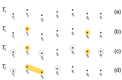
Figure 1: (a) Trajectory $T_{1}$, (b) The pivots of size one, (c) The pivots neighborhood, and (d) one pivot of size two neighborhood.

Algorithm 3 presents the pivots strategy. First, it generates the candidates of size one (line 6), assess their relative frequency (line 8), sort in descending quality order (line 9) and than filter the candidates relative frequency inferior of $\tau$ (line 11). Then, it looks for candidates of size two from the neighborhood of the previous candidates of size one (line 6), and prunes again by low relative frequency (line 11). The findCandidates function (line 6) will generate subtrajectories from the previous size candidates adding the neighbor point in the beginning or end. It goes on increasing the size until it reaches the trajectory size limit (line 5).

Algorithm 3 hiperExtraction // With Pivots

1:Input: $\textit{T}_{k}$ // a trajectory,

2:         T’ // Trajectory set for the class,

3:Output: bestCandidates // set of best hiper candidates

4:           bucket // set of the remaining movelet candidates

5:$\textit{bestCandidates}\leftarrow\emptyset$

6:$\textit{candidates}_{size}\leftarrow\emptyset$

7:$\textit{bucket}\leftarrow\emptyset$

8:$m\leftarrow\textit{T}_{i}.length$              // OR $\log_{2}\left(\textit{T}_{i}.length\right)$

9:for size in $(1,m)$ do

10:     $\textit{candidates}_{T_{i}}\leftarrow findCandidates(T_{i},\textit{candidates}_{size},size)$

11:     for each $\mathcal{M}\;\textbf{in}\;\textit{candidates}_{T_{i}}$ do

12:         $\mathcal{M}.L.quality\leftarrow quality_{freq}(\mathcal{M},\textbf{T'})$      

13:     $\textit{candidates}_{T_{i}}.sort()$

14:     $\tau\leftarrow\textit{candidates}_{T_{i}}[0].L.quality\;*\;\operatorname{0.5}$

15:     $\textit{candidates}_{size}\leftarrow moveletCandidatePruning(\textit{candidates}_{T_{i}},\textbf{T'},\tau)$

16:     $\textit{bestCandidates}\leftarrow\textit{bestCandidates}\cup\textit{candidates}_{size}$

17:     $\textit{bucket}\leftarrow\textit{bucket}\cup(\textit{candidates}_{T_{i}}-\textit{candidates}_{size})$

18:$\textbf{return}{}\ \textit{bestCandidates},\;\textit{bucket}$

When a dataset has more dimensions, more patterns can be found and it is easier to find discriminant movelets. Indeed, the more is information available with combined dimensions, the more unique behaviours can be found. For instance, datasets with one dimension are harder for finding discriminating patterns in classes and HiPerMovelets might end not finding movelets among the better qualified candidates. HiPerMovelets keeps the set of removed candidates($bucket$ in Algorithm 3 line 13), and it will use the $bucket$ set to look for movelets in case none was previously found.

3.1.3 Movelets Discovery

The movelets discovery is similar to MASTERMovelets algorithm [3], it computes and filters the movelet candidates using the F-Score quality. The difference is that our method only calculates this quality for the class-frequent movelet candidates. To measure the F-Score is necessary to compare each candidate with the entire dataset, and by reducing the number of movelet candidates, this task can be done significantly faster.

This step is represented by the subroutine moveletDiscovery in Algorithm 1 (line 7), in which the movelets are the best representations of the behaviors of a class. First, it filters candidates that are equal, what can happen when a behavior repeats in the same trajectory. Then, HiPerMovelets calculates distances for all movelet candidates to the dataset trajectories, and assesses their F-Score quality. Then, candidates with zero quality and overlapping points are discarded. If the resulting movelets are an empty set, the HiPerMovelets will repeat this step with the $bucket$ set of candidates previously excluded. Only the movelet candidates with best quality and without point overlapping in the trajectory are kept and called movelets.

3.1.4 Trajectory Pruning

From the discovered movelets of each trajectory, HiPerMovelets evaluates the covered trajectories. Algorithm 4 shows how our method finds covered trajectories from the movelets of trajectory $T_{i}$ (line 3). First, each trajectory is mapped with the number of occurrences in the movelets coverage (lines 4 to 5). Then, it selects the trajectories covered by at least half of the movelets (lines 6 to 8). If a class contains similar trajectories, than HiPerMovelets search space can be reduced as the movelets will cover more examples (trajectories) in the class. However, classes with distant trajectories will need more examples to discover movelets.

Algorithm 4 coveredTrajectories

1:Input: $\textbf{M}^{T_{i}}$ // set of movelets of trajectory $T_{i}$

2:Output: covered // set of covered trajectories

3:$\textit{covered}\leftarrow\emptyset$

4:$covered\_count\leftarrow Map[]$

5:for each movelet in $\textbf{M}^{T_{i}}$ do

6:     for each $\textit{T}_{x}$ in $\textit{movelet}.coveredTrajectories$ do

7:         $covered\_count[\textit{T}_{x}]++$      

8:for each $\textit{T}_{y}$ in $covered\_count$ do

9:     if $covered\_count[\textit{T}_{y}]>(|\textbf{M}^{T_{i}}|/2)$ then

10:         $\textit{covered}\leftarrow\textit{covered}\;\cup\;\textit{T}_{y}$      

11:return  covered

4 Experimental Evaluation

We evaluated the HiPer Movelets approach by comparing their computational cost and classification power. First, we evaluated their computational cost in learning the model, and the classification power with MASTERMovelets-Log.

4.1 Datasets

We performed preliminary experiments with the datasets of multiple aspect trajectories to evaluate used in [3, 6, 19]. They are composed of check-in trajectories and are enriched with semantic dimensions from three different Location-Based Social Networks (LBSN). The trajectories were splitted by week in order to increase the trajectories examples of each user as necessary for classification tasks. The multiple aspect trajectory datasets were used for evaluating the HiPerMovelets, because of their number of dimensions and because MASTERMovelets-Log was tested with these datasets. We evaluated our method over the same datasets used in [3, 6], with the average trajectory size, the number of trajectories, points and classes, and the attributes of the dataset. We also evaluated this datasets using only the spatial dimension, referred as “spatial only”.

Brightkite: dataset from Brightkite social media, collected between April 2008 and October 2010 [20]. A total of $300$ users were randomly selected, with a total of $7,911$ trajectories, a minimum of $10$ points and maximun of $50$ points per trajectory for consistency. Trajectories provide the anonymized user of the check-in, the POI, space and time information, and were enriched with the semantic weekday information.

Gowalla: dataset from the Gowalla Location-Based Social Network (LSBN), collected between February 2009 and October 2010 [20]. We used a total of $300$ random users for analysis, limiting the trajectory sizes of minimum $10$ and maximun $50$ points, resulting in a total of $5,329$ trajectories. It is composed by the same dimensions as the Brightkite dataset, including the enriched semantic information of the weekday.

The Foursquare dataset is from the Foursquare social media, having the user check-in, the POI and the spatial position in time when the check-in was made. Trajectories were enriched with semantic information of: (i) the weekday, (ii) the POI from the Foursquare API with the POI category, and the numerical information of its price and rating. The trajectories were splitted in weeks to increase the examples for each user with at least $10$ check-ins.

Foursquare NYC: the dataset was collected between April 2012 and February 2013 [21]. It has a total of $227,428$ check-in points of $1,083$ users in New York, USA. It provides $193$ users for this dataset. The dataset has a total of $3079$ trajectories, with trajectory sizes varying from $10$ to $144$. The dataset trajectories were enriched with the weather information at the POI location and time with the Weather Wunderground API.

4.2 Experimental Setup

The datasets are split in a hold-out proportion of $70\%$ training and $30\%$ testing, with respect to the class balance. We evaluated three classification models: the Multilayer-Perceptron (MLP), the Random Forest (RF) and the Support Vector Machine (SVM), as they are commonly used and achieved good results in [3, 6, 19]. The classifiers were implemented using the Python language, with the keras package in the same way as [3, 19]. The MLP has a fully-connected hidden layer with $100$ units, a Dropout Layer rate of $0.5$, learning rate of $10^{-}3$ and Output Layer with softmax activation. It was also applied Adam Optmization to improve the learning time and to avoid categorical cross entropy loss, same as in the work of [19], with $200$ of batch size, and a total of $200$ epochs for each training. The Random Forest was built with $300$ decisions trees. The Support Vector Machine (SVM) algorithm was implemented with linear kernel, and probability estimates are enabled.

In the MASTERMovelets configurations, the distance was calculated in each dimension by using: (i) euclidean distance for the space, (ii) difference for the numerical, and (iii) simple equality (if is equal or not) for the semantical.

The experiments were performed in an Intel(R) Core(TM) i7-9700 CPU @ 3.00GHz, with $8$ cores (limited to $3$ threads) and 32GB of intern memory.

4.3 Preliminary Results

We compared the classification results of the MASTERMovelets-Log and our approaches, by using the Accuracy metric. The results for each dataset are presented in Table 1, where the higher values for each metric are presented in bold, and the second best are underlined. MARC was the fastest method in almost all the experiments, but its running time is not compared as HiPerMovelets and MASTERMovelets methods, as they were limited to three threads for a fair time comparison between them. In addition, MARC had the eight cores and GPU acceleration to run.

In this experiment we compare the number of movelet candidates generated by the MASTERMovelets-Log and HiPerMovelets-Log, the number of movelets, the time spent in this task, the accuracy and time of classification in each classifier, and the HiPerMovelets-Log number of trajectories it looked for movelets extraction. Table 1 summarizes the results, where the main observation is that the method HiPerMovelets-Pivots-Log is at least $95\%$ faster than the MASTERMovelets-Log in time comparison in any of the specific datasets, and HiPerMovelets-Log is at least $71\%$ faster in the same datasets. HiPerMovelets-Pivots-Log and HiPerMovelets-Log in the spatial only datasets are, respectively, at least $78\%$ and $70\%$ faster than MASTERMovelets-Log. Note that in the spatial only dataset of Foursquare NYC MASTERMovelets-Log did not output movelets.

Table 1: Results for Brightkite, Gowalla and Foursquare NYC datasets.

Dataset		MARC	MASTER. -Log	HiPer. -Log	HiPer. Pivots -Log
Brightkite (spatial only)	Candidates	-	409,380	288,319	192,811
	Movelets	-	83,422	38,186	39,802
	MLP	94.158	94.849	94.033	93.970
	RF		94.095	93.342	93.530
	SVM		93.970	93.342	93.279
	Extraction Time	8m48s	1h16m15s	22m49s	18m12s
	Time MLP		36m44s	14m38s	15m09s
	Time RF		28s	16s	17s
	Time SVM		1h51m36s	41m05s	43m07s
	Trajs. Compared	-	-	4,549	4,617
	Trajs. Pruned	-	-	1,770	1,702
Gowalla (spatial only)	Candidates	-	318,326	252,281	146,825
	Movelets	-	52,711	11,860	12,380
	MLP	87.723	94.752	90.628	91.753
	RF		91.565	89.784	90.159
	SVM		91.471	88.004	87.629
	Extraction Time	5m58s	42m54s	4m44s	6m54s
	Time MLP		12m23s	2m52s	2m59s
	Time RF		14s	6s	6s
	Time SVM		1h18m20s	12m16s	12m52s
	Trajs. Compared	-	-	3,381	3,345
	Trajs. Pruned	-	-	881	917
Foursquare NYC (spatial only)	Candidates	-	240,297	181,549	108,418
	Movelets	-	0	7,521	7,411
	MLP	92.241	-	91.552	91.034
	RF		-	89.828	89.655
	SVM		-	88.966	88.621
	Extraction Time	8m08s	9m36s	1m53s	1m44s
	Time MLP		-	1m05s	1m03s
	Time RF		-	3s	2s
	Time SVM		-	2m47s	2m40s
	Trajs. Compared	-	-	1,897	1,893
	Trajs. Pruned	-	-	602	606

Dataset		MARC	MASTER. -Log	HiPer. -Log	HiPer. Pivots -Log
Brightkite (specific)	Candidates	-	6,140,700	3,355,050	773,364
	Movelets	-	88,763	34,586	33,280
	MLP	95.477	96.420	96.357	95.729
	RF		95.352	95.791	95.415
	SVM		95.854	95.791	95.603
	Extraction Time	6m26s	22h48m01s	2h40m07s	36m00s
	Time MLP		38m40s	13m15s	12m46s
	Time RF		22s	12s	12s
	Time SVM		4h21m54s	1h55m01s	1h46m07s
	Trajs. Compared	-	-	3,657	3,299
	Trajs. Pruned	-	-	2,662	3,020
Gowalla (specific)	Candidates	-	4,774,890	3,064,335	607,977
	Movelets	-	62,141	20,312	17,459
	MLP	95.314	95.689	94.564	94.845
	RF		94.283	93.440	92.784
	SVM		92.596	88.379	89.503
	Extraction Time	11m13s	9h23m59s	54m26s	14m01s
	T. MLP		14m35s	4m59s	4m16s
	T. RF		14s	8s	7s
	T. SVM		2h00m42s	47m04s	38m48s
	Trajs. Compared	-	-	2,765	2,318
	Trajs. Pruned	-	-	1,497	1,944
Foursquare NYC (specific)	Candidates	-	61,275,735	25,697,880	3,248,927
	Movelets	-	36,353	14,956	11,552
	MLP	98.966	97.069	98.276	95.345
	RF		95.345	96.552	96.552
	SVM		90.862	83.793	74.138
	Extraction Time	9m09s	29h49m49s	8h32m47s	1h28m02s
	T. MLP		4m50s	. 2m05s	1m37s
	T. RF		4s	3s	4s
	T. SVM		34m24s	. 14m44s	11m15s
	Trajs. Looked	-	-	1,173	674
	Trajs. Pruned	-	-	1,326	1,825

MASTERMovelets-Log has the highest accuracy in almost all experiments. In the specific and spatial only datasets, however, our method had almost the same or higher accuracy than MASTERMovelets-Log.

5 Conclusion

In this draft we proposed a method for fast movelet extraction, that is more efficient than MasterMovelets and keeps a similar accuracy. In future works we will perform several experiments with 5-fold cross validation and scalability analysis.

References

- [1] Jae Gil Lee, Jiawei Han, Xiaolei Li, and Hector Gonzalez. TraClass: Trajectory classification using hierarchical region based and trajectory based clustering. Proceedings of the VLDB Endowment, 1(1):1081–1094, 2008.
- [2] Mohammad Etemad, Amílcar Soares Júnior, and Stan Matwin. Predicting transportation modes of GPS trajectories using feature engineering and noise removal. Lecture Notes in Computer Science (including subseries Lecture Notes in Artificial Intelligence and Lecture Notes in Bioinformatics), 10832 LNAI(ii):259–264, 2018.
- [3] Carlos Andres Ferrero, Lucas May Petry, Luis Otávio Alvares, Camila Leite da Silva, Willian Zalewski, and Vania Bogorny. MasterMovelets: discovering heterogeneous movelets for multiple aspect trajectory classification. Data Min. Knowl. Discov., 34(3):652–680, 2020.
- [4] Carlos Andres Ferrero, Luis Otavio Alvares, Willian Zalewski, and Vania Bogorny. Movelets: Exploring relevant subtrajectories for robust trajectory classification. In Proceedings of the 33rd Annual ACM Symposium on Applied Computing, SAC ’18, page 849–856, New York, NY, USA, 2018. Association for Computing Machinery.
- [5] Francisco Vicenzi, Lucas May Petry, Camila Leite Da Silva, Luis Otavio Alvares, and Vania Bogorny. Exploring frequency-based approaches for efficient trajectory classification. Proceedings of the ACM Symposium on Applied Computing, pages 624–631, 2020.
- [6] Lucas May Petry, Camila Leite da Silva, Andrea Esuli, Chiara Renso, and Vania Bogorny. MARC: a robust method for multiple-aspect trajectory classification via space, time, and semantic embeddings. International Journal of Geographical Information Science, 2020.
- [7] Tomas Mikolov, Ilya Sutskever, Kai Chen, Greg S Corrado, and Jeff Dean. Distributed representations of words and phrases and their compositionality. In Advances in neural information processing systems, pages 3111–3119, 2013.
- [8] Gustavo Niemeyer. Geohash. [Online]. Available: https://en.wikipedia.org/wiki/Geohash, 2008.
- [9] Sina Dabiri and Kevin Heaslip. Inferring transportation modes from GPS trajectories using a convolutional neural network. Transportation Research Part C: Emerging Technologies, 86(August 2017):360–371, 2018.
- [10] Zhibin Xiao, Yang Wang, Kun Fu, and Fan Wu. Identifying different transportation modes from trajectory data using tree-based ensemble classifiers. ISPRS International Journal of Geo-Information, 6(2), 2017.
- [11] Irineu Júnior Pinheiro dos Santos, Irineu Jr, and Luis Otavio Alvares. TRACTS: um método para classificação de trajetórias de objetos móveis usando séries temporais. In XXXI Congresso da Sociedade Brasileira de Computação, 2011.
- [12] Lexiang Ye and Eamonn Keogh. Time series shapelets: A novel technique that allows accurate, interpretable and fast classification. Data Mining and Knowledge Discovery, 22(1-2):149–182, 2011.
- [13] Abdullah Mueen, Eamonn Keogh, and Neal Young. Logical-shapelets: An expressive primitive for time series classification. Proceedings of the ACM SIGKDD International Conference on Knowledge Discovery and Data Mining, pages 1154–1162, 2011.
- [14] Thanawin Rakthanmanon and Eamonn Keogh. Fast shapelets: A scalable algorithm for discovering time series shapelets. Proceedings of the 2013 SIAM International Conference on Data Mining, SDM 2013, pages 668–676, 2013.
- [15] Cun Ji, Chao Zhao, Shijun Liu, Chenglei Yang, Li Pan, Lei Wu, and Xiangxu Meng. A fast shapelet selection algorithm for time series classification. Computer Networks, 148:231–240, 2019.
- [16] J. Zuo, K. Zeitouni, and Y. Taher. SE4TeC: A scalable engine for efficient and expressive time series classification. CEUR Workshop Proceedings, 2343:8–12, 2018.
- [17] Zhenguo Zhang, Haiwei Zhang, Yanlong Wen, Ying Zhang, and Xiaojie Yuan. Discriminative extraction of features from time series. Neurocomputing, 275:2317–2328, 2018.
- [18] Andrea Gigli, Claudio Lucchese, Franco Maria Nardini, and Raffaele Perego. Fast feature selection for learning to rank. ICTIR 2016 - Proceedings of the 2016 ACM International Conference on the Theory of Information Retrieval, pages 167–170, 2016.
- [19] Camila Leite da Silva. Pivot-based approaches for Movelets and MASTERMovelets Optimizations. Master thesis, Universidade Federal de Santa Catarina, Florianópolis, SC, Brasil, 2020.
- [20] Eunjoon Cho, Seth A. Myers, and Jure Leskovec. Friendship and mobility: User movement in location-based social networks. Proceedings of the ACM SIGKDD International Conference on Knowledge Discovery and Data Mining, pages 1082–1090, 2011.
- [21] D Yang, D Zhang, V W Zheng, and Z Yu. Modeling User Activity Preference by Leveraging User Spatial Temporal Characteristics in LBSNs. IEEE Transactions on Systems, Man, and Cybernetics: Systems, 45(1):129–142, 2015.