Towards photoassociation processes of ultracold rubidium trimers

Abstract

We theoretically investigate the prospects for photoassociation (PA) of Rb3, in particular at close range. We provide an overview of accessible states and possible transitions. The major focus is placed on the calculation of equilibrium structures, the survey of spin-orbit effects and the investigation of transition dipole moments. Furthermore we discuss Franck-Condon overlaps and special aspects of trimers including the (pseudo) Jahn-Teller effect and the resulting topology of adiabatic potential-energy surfaces. With this we identify concrete and suitable PA transitions to potentially produce long-lived trimer bound states. Calculations are performed using the multireference configuration-interaction method together with a large-core effective core potential and a core-polarization potential with a large uncontracted even-tempered basis set.

I Introduction

Ultracold molecules offer great opportunities for research and applications, as they can be prepared in precisely defined quantum states Quemener and Julienne (2012); Bohn et al. (2017); Balakrishnan (2016); Krems (2008); Carr et al. (2009); Doyle et al. (2004). Besides studying the molecular properties with high precision, collisions and chemical reactions can then be investigated in the quantum regime where only a single partial wave contributes. Furthermore, cold molecules have a number of applications, ranging from metrology to quantum sensors, to quantum simulation and computation Bohn et al. (2017); Carr et al. (2009). In recent years a number of ways to produce cold molecules have been developed ranging from buffer gas cooling, slowing and filtering, laser cooling, to associating ultracold atoms. The coolest temperatures and the highest control in preparing the molecular quantum state have been typically achieved by associating ultracold atoms Quemener and Julienne (2012); Balakrishnan (2016); Krems (2008). In this way a variety of different ultracold diatomic molecules has been produced, typically consisting of alkali-atoms, such as Li2, Na2, K2, Rb2, Cs2, NaRb, RbCs, RbK, NaK, LiNa, LiK, LiRb, LiCs, NaCs, but there are also other compounds, such as LiYb, RbYb, see, e.g. Refs. Bohn et al. (2017); Balakrishnan (2016); Krems (2008); Doyle et al. (2004) and references therein. Possible methods for the molecule production are e.g., three-body recombination Burt et al. (1997); Stamper-Kurn et al. (1998); Greene et al. (2017), photoassociation Ulmanis et al. (2012); Jones et al. (2006), and sweeping over a Feshbach resonance Köhler et al. (2006); Chin et al. (2010).

Alkali metal dimer systems have also been studied theoretically in great detail. Accurate potential energy curves (PECs), dipole moments and spin-orbit interactions can be obtained via several ab initio methods Dulieu and Gabbanini (2009). Among others, the Fourier Grid Hamiltonian method Kosloff (1988); Dulieu and Julienne (1995) or the discrete variable representation (DVR) method Colbert and Miller (1992) were used to analyze the level structure of the well-known coupled $\mathrm{A}\,\tensor{*}[^{1}]{\Sigma}{{}_{u}^{+}}$–$\mathrm{b}\,\tensor{*}[^{3}]{\Pi}{{}_{u}}$ manifold in homonuclear alkali metal dimers.

Producing and understanding ultracold alkali trimers (i.e., e.g.: $\mathrm{X}_{2}\mathrm{Y}$, $\mathrm{X}_{3}$, etc. with $\mathrm{X},\mathrm{Y}\in\{\ce{Li},\ce{Na},\ce{K},\ce{Rb},\ce{Cs}\}$) clearly is a next milestone. Alkali trimers are much more complex and challenging as compared to alkali dimers, both from the theoretical and the experimental point of view. One aspect of the complexity of an alkali trimer is that many of its levels are prone to quick decay due to fast internal relaxation and dissociation mechanisms. This makes it challenging to prepare and manipulate the trimer on the quantum level. Indeed, detailed and highly resolved spectroscopy on free trimer molecules is generally still lacking. Ultracold trimers have not been produced yet, apart from the extremely weakly-bound Efimov states Greene et al. (2017); Ferlaino et al. (2011), which are fast-decaying three-body states of resonantly interacting atoms. Alkali trimers at mK-temperatures, however, have been produced in experiments using supersonic beam expansion of Ar seeded with, e.g. sodium atoms, as in Refs. Delacrétaz et al. (1986); Ernst and Rakowsky (1995); Vituccio et al. (1997), or in experiments with alkali metal clusters formed on helium droplets Nagl et al. (2008a); Auböck et al. (2008); Nagl et al. (2008b); Hauser and Ernst (2011); Giese et al. (2011). Theoretical interest in alkali metal clusters already goes back to the 80s and 90s, with a number of pioneering works Martin and Davidson (1978); Martins et al. (1983); Thompson et al. (1985); Cocchini et al. (1988); Spiegelmann and Pavolini (1988); Meiswinkel and Köppel (1990); de Vivie-Riedle et al. (1997) giving insights into the electronic properties of alkali trimers, the corresponding ground state potential energy surfaces (PESs) and the occurring Jahn-Teller (JT) effect. Yet, these studies were restricted to light alkali metal species, i.e. Li, Na and K. Later, following the success of the helium droplet method, theoretical investigations of alkali trimer systems were reappearing – now also containing heavier elements such as Rb Hauser et al. (2008, 2010a, 2010b, 2015, 2009); Hauser (2009); Soldán (2010). In these works, the main focus was on selected JT states and the reproduction of special transitions and spectra measured with He-droplet spectroscopy. In recent years, the advent of experiments studying ultracold collisions between an alkali atom and an alkali dimer also triggered further calculations of ground state alkali trimer PESs. For an overview see, e.g. Quemener and Julienne (2012).

A promising approach for preparing isolated trimer molecules in precisely defined quantum states is photoassociation (PA) which so far has been used for creating dimers in the ultracold regime Ulmanis et al. (2012); Jones et al. (2006). In a PA process a colliding atom pair in the electronic ground state and a laser photon is transferred into a well-defined bound, electronically excited state $\ket{e}$ Jones et al. (2006). From there, the excited molecule can spontaneously decay into a number of ro-vibrational, long-lived levels of the molecular ground state manifold $\ket{g}$. In analogy, one can in principle think of two possible PA schemes for the production of trimer molecules, cf. Fig. 1:

• A dimer molecule and a free ground-state atom are photoassociated ($\equiv$ PA 1). This is shown in Fig. 1. The laser photon drives a transition from the asymptote $\ket{g_{1}}$ to an electronically excited bound state $\ket{e}$ of the trimer complex. From there it can spontaneously relax to the ground state.

• Three colliding free atoms are photoassociated ($\equiv$ PA 2). As shown in Fig. 1, the photon drives the transition now from the asymptote $\ket{g_{2}}$ to the excited trimer state.

The PA can in principle take place at long range (large internuclear distances) or at short range (small internuclear distances).

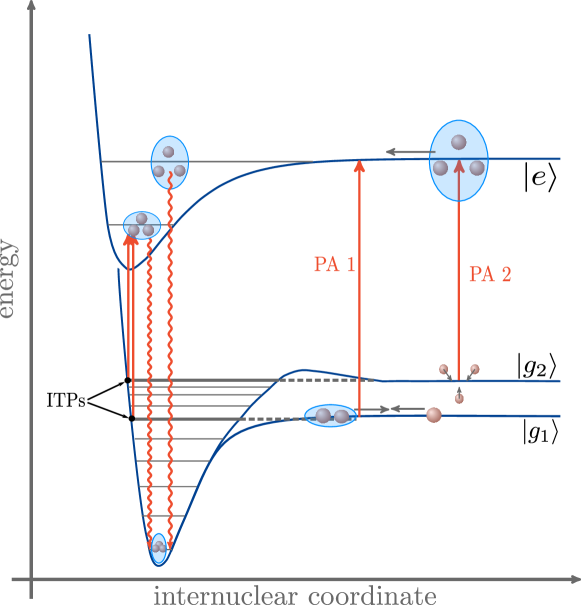
Figure 1: (Color online) Strongly simplified illustration of the two different photoassociation (PA) schemes for the production of Rb3 species. PA 1 photoassociates a Rb2 dimer with a free Rb atom starting from the asymptote $\ket{g_{1}}$. PA 2 photoassociates three Rb atoms starting from the asymptote $\ket{g_{2}}$. Both PA processes can be also realized (in principle) starting from an inner turning point (ITP), as discussed in Sec. III.1 and indicated on the very left. In both cases the excited trimer (more weakly bound for PA starting from $\ket{g_{1}}$ or $\ket{g_{2}}$) can radiatively decay to the ground state.

Photoassociation at large distances was recently discussed theoretically in Pérez-Ríos et al. (2015). Here, we therefore rather focus on trimer photoassociation at short distances. Recent theoretical work in Ref. Wang et al. (2012), however, suggests that the simultaneous collision of three atoms is strongly suppressed due to an effective repulsive barrier in the short-range of the three-body potential, rendering the realization of PA2 at short range less likely. For PA1, however, such a restriction is not expected. Working out concrete schemes for trimer PA requires detailed knowledge of the involved trimer states and the optical transitions between them. With the present work we provide a broad overview of states in terms of energy levels and the topology of potential energy surfaces (PESs). Previous theoretical studies on alkali trimers Hauser and Ernst (2011); Giese et al. (2011); Martin and Davidson (1978); Martins et al. (1983); Thompson et al. (1985); Cocchini et al. (1988); Spiegelmann and Pavolini (1988); Meiswinkel and Köppel (1990); de Vivie-Riedle et al. (1997); Mukherjee and Adhikari (2014); Hauser et al. (2008, 2010a, 2010b, 2015, 2009); Hauser (2009) were essentially restricted to either the doublet or quartet ground state or they investigated selected JT distorted excited states. Furthermore, we calculate the electronic dipole transition matrix elements between states. We discuss special aspects of trimers including different coordinate systems, the (pseudo) Jahn-Teller effect, the Renner-Teller effect for linear configurations, as well as accidental degeneracies. Finally, we suggest specific PA transitions and investigate coupling effects in terms of spin-orbit interaction. Our work is intended as a basis for further detailed investigations of PA, which at the next stage will require the simulation of nuclear dynamics.

This work is organized as follows. Section II briefly introduces the computational aspects and convenient coordinate systems for trimers. Hereafter we discuss major topological features of the corresponding PESs by means of special cuts and comment on the (pseudo) Jahn-Teller (and Renner-Teller) effect. Here, we additionally provide an overview of the expected quartet and doublet equilibrium states of the trimer system within a certain energy range and comment on spin-orbit coupling effects and estimate their magnitude. In Sec. III we analyze the excited electronic states with regard to their applicability in PA processes. We find that they can be reached conveniently via the inner-turning points on the quartet ground state PES. We identify one component of the $1{\,}\tensor{*}[^{4}]{\mathrm{E}}{{}^{\prime\prime}}$ Jahn-Teller pair as a promising candidate for PA experiments. We thoroughly investigate its suitability as a target state by studying electronic transition dipole strengths with the quartet ground state, spin-orbit coupling and further mixing effects with other states in its close proximity, as well as its distance from conical intersections (COINs). Finally, we summarize the main points of this work in Sec. IV and give an outlook to ongoing work.

II General Overview of the Rubidium Trimer System

II.1 Computational Aspects

Table 1: Comparison of experimental (references given in square brackets) and calculated values for some spectroscopic constants of a few Rb2 states. $D_{e}$ is the dissociation energy, $R_{e}$ the equilibrium distance, and $T_{e}$ the electronic term energy. Calculations are performed at MRCI(ECP+CPP)/15s12p7d5f3g level of theory. We also report differences $\Delta$ between theory and experiment as well as the mean difference $\bar{\Delta}$ and the absolute mean difference $\bar{\Delta}_{\text{abs}}$ for the given set of states.

State	$D_{e}\,[\mathrm{cm}^{-1}]$			$R_{e}\,[$\mathrm{\SIUnitSymbolAngstrom}$]$			$T_{e}\,[\mathrm{cm}^{-1}]$
	this work	exp.	$\Delta$	this work	exp.	$\Delta$	this work	exp.	$\Delta$
$\mathrm{X}{\,}\tensor{*}[^{1}]{\Sigma}{{}_{g}}\;$ Strauss et al. (2010)	$4116$	$3993.593$	$122$	$4.1689$	$4.2099$	$-0.0410$	$0$	$0$	$0$
$\mathrm{a}{\,}\tensor{*}[^{3}]{\Sigma}{{}_{u}}\;$ Strauss et al. (2010)	$250$	$241.503$	$8$	$6.0065$	$6.0940$	$-0.0875$	$3866$	–	–
$\mathrm{b}{\,}\tensor{*}[^{3}]{\Pi}{{}_{u}}\;$  Salami et al. (2009)	$7218$	$7039$	$179$	$4.1537$	$4.1329$	$0.0208$	$9632$	$9601$	$31$
$\mathrm{A}{\,}\tensor{*}[^{1}]{\Sigma}{{}_{u}}\;$ Salami et al. (2009)	$6071$	$5981$	$90$	$4.8637$	$4.8737$	$-0.0100$	$10\,778$	$10\,750$	$28$
$(2){\,}\tensor{*}[^{1}]{\Sigma}{{}_{g}}\;$ Drews et al. (2017); Amiot and Verges (1987)	$3140$	$2963$	$177$	$5.4081$	$5.4399$	$-0.0318$	$13\,709$	$13\,602$	$107$
$(1){\,}\tensor{*}[^{1}]{\Pi}{{}_{u}}\;$ Amiot (1990)	$2150$	$1907$	$243$	$4.5203$	–	–	$14\,700$	$14\,666$	$34$
$(1){\,}\tensor{*}[^{1}]{\Pi}{{}_{g}}\;$ Amiot (1986)	$1246$	$1290$	$-44$	$5.4225$	$5.4188$	$0.0037$	$15\,604$	$15\,510$	$94$
		$\mathrm{bar}{\Delta}:$	$111$			$-0.0243$			$59$
		$\mathrm{bar}{\Delta}_{\text{abs}}:$	$123$			$0.0325$			$59$

Since investigating PA processes of Rb3 requires an extensive survey of a large number of expected states and transitions in the Rb3 system, a pragmatic but considerably accurate computational approach has to be applied. In this work, we are using a large-core effective core potential (ECP) in combination with a core polarization potential (CPP) as it has been developed in Ref. Silberbach et al. (1986) with a large [15s12p7d5f3g] (uncontracted and even-tempered) basis set (UET15) – see supplementary material Sup for details. In doing so merely the valence electron of Rb is treated explicitly while the remaining 36 electrons are described by the ECP. The CPP accounts for dynamic polarization of the core electrons by the valence electrons. All doublet and quartet states of Rb3 within a certain energy range were computed using the internally contracted multireference configuration interaction (MRCI) method Werner and Knowles (1988); Knowles and Werner (1988, 1992); Werner and Reinsch (1982); Werner (1987). As we are only dealing with an effective three-electron system, the MRCI method has no problem with the separability of the wavefunction. This means that the PESs are entirely well defined and show correct dissociation behavior into three non-interacting Rb atoms. All calculations are performed using the molpro 2018.2 program package Werner et al. (2018).

The pragmatic ECP$+$CPP approximation is sufficient for gaining a reliable understanding of the physics of the system, as shown in the following, while saving tremendously on computational costs. By construction, the ECP reproduces the experimentally determined atomic energy levels up to the ${}^{2}\mathrm{F}$ state Silberbach et al. (1986). The results in Tab. 1 illustrate the expected accuracy for molecular systems – here in terms of benchmark calculations for spectroscopic constants of selected singlet and triplet states of Rb2 in comparison to experimental results. The calculations do not account for spin orbit coupling effects, which are only rather small perturbations in most cases. This we will also show in the present study for Rb3. The mean differences $\bar{\Delta}$ reported in Tab. 1 show a systematic overestimation of the binding energies by $100$ to $250\,\mathrm{cm}^{-1}$, while equilibrium distances are typically underestimated by $0.01$ to $0.04\,$\mathrm{\SIUnitSymbolAngstrom}$$. This over- and underestimation is a well-known bias introduced by the large-core ECPs due to the approximate description of the repulsion of the core electrons Jeung (1997); Guérout et al. (2009). For the electronic term energies $T_{e}$, the errors are on the order of $30$ to $100\,\mathrm{cm}^{-1}$. Since the Rb3 system forms three Rb-Rb bonds, we can estimate the accuracy of our ab initio method from the above mean errors by $\approx\pm 300\,\mathrm{cm}^{-1}$. For bond lengths the same accuracy as for Rb2 is expected (about 1 per cent of the total predicted distance). According to the above experience, binding energies are probably mostly overestimated while bond lengths are underestimated. While these deviations seem large from a spectroscopist’s point of view, we note that these deviations are already within the regime of accurate quantum chemical methods, typically defined by the ’chemical accuracy’ level of $\approx\pm 1\,\mathrm{kcal}/\mathrm{mol}\approx\pm 350\,\mathrm{cm}^{-1}$ for energies. Increasing this accuracy is possible but requires steeply increasing computational resources, while our present approach only requires approximately 40 minutes on 8 cores for solving for 27 electronic states at a given Rb3 geometry, thus allowing to explore the configurational space efficiently.

II.2 Coordinates

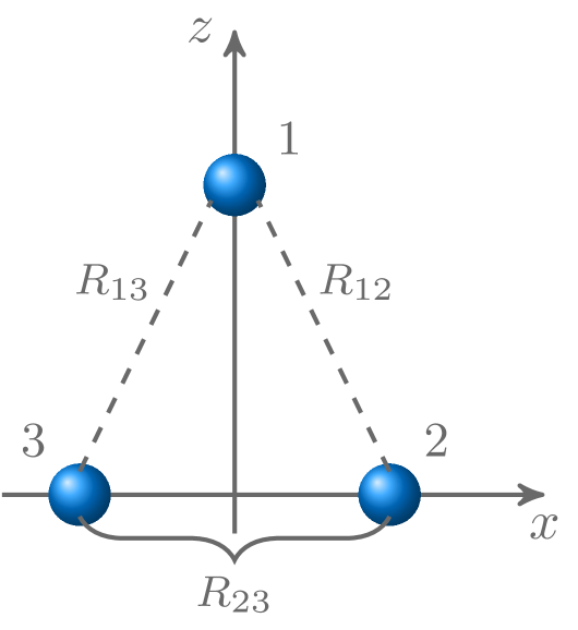
(a)

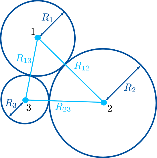
(b)

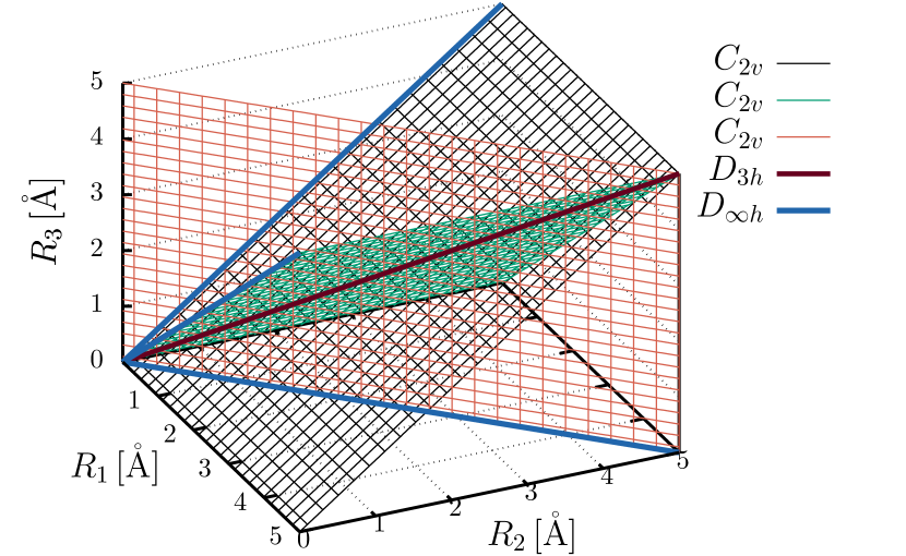
(c)

Figure 2: (Color online) (a) Sketch of the Rb3 system in the $xz$ plane with internuclear distances $R_{12},R_{23},R_{13}$. (b) Illustration of the geometric interpretation of the perimetric coordinates for triatomic molecules. They represent the radii of three mutual tangent circles centered on the nuclei. (c) Division of the positive octant in perimetric coordinates to show special configuration subspaces of triatomic systems (i.e. $D_{\infty h}$, $D_{3h}$ and $C_{2v}$).

The atoms of non-linear triatomic molecular systems always define a plane, which we choose, without loss of generality, as the $xz$ plane, see Fig. 2 (a). The system has three internal degrees of freedom, with the only exception of linear geometries for which the system has a fourth degree of freedom. There are many coordinate systems available for properly studying the physics of the system – like the well-known Jacobi and hyperspherical coordinates, see, e.g. Ref. Suno et al. (2002) and references therein. In general every coordinate system has its strengths and weaknesses and the choice strongly depends on what one wants to analyze. In this work we are making use of three different coordinate systems which are introduced in the following.

It is straightforward to use internuclear distances as shown in Fig. 2 (a). However, not every triple of numbers $(R_{12},R_{23},R_{13})$ obeys the triangular condition and defines a possible molecular configuration. It is convenient to employ perimetric coordinates Coolidge and James (1937); Pekeris (1958, 1959); Pekeris et al. (1962); Pekeris (1962); Accad et al. (1971); Schiff et al. (1971), as used by Davidson in his analysis of H3 Davidson (1977). Given the set of internal coordinates $\{R_{12},R_{23},R_{13}\}$, the perimetric coordinates can be expressed as

$$R_{1} =\frac{1}{2}\left(R_{12}+R_{13}-R_{23}\right)$$ (1a)

$$R_{2} =\frac{1}{2}\left(R_{12}+R_{23}-R_{13}\right)$$ (1b)

$$R_{3} =\frac{1}{2}\left(R_{13}+R_{23}-R_{12}\right)\,.$$ (1c)

The perimetric coordinates are the radii of mutually tangent circles centered on each nucleus (as shown in Fig. 2 (b)). The general topology of this coordinate system reveals some properties:

1. Every triple of numbers ($R_{1},R_{2},R_{3}$) in the positive octant (cf. Fig. 2 (c)) gives a unique molecular conformation (modulo permutational inversion); i.e. the coordinates satisfy the triangular inequality

2. Internuclear distances are given as the sum of the corresponding perimetric coordinates (e.g. $R_{12}=R_{1}+R_{2}$)

3. Linear molecules are found at the three equivalent boundary planes of the positive octant, where one of the perimetric coordinates is zero (e.g. for $R_{1}=0$, $R_{2}=R_{12}$ and $R_{3}=R_{13}$).

4. The dissociation limits (atom $+$ dimer) are obtained by one of the coordinates being large (e.g. $\mathrm{atom}_{1}+\mathrm{dimer}_{23}\Leftrightarrow R_{1}\to\infty$).

The positive octant contains further special positions (i.e. configurations higher than $C_{s}$ symmetry) summarized in Fig. 2 (c). Linear molecules of $D_{\infty h}$ symmetry are found on three equivalent diagonals of the boundary planes. Equilateral triangular configurations ($D_{3h}$ symmetry) correspond to the space diagonal while isosceles triangles (i.e. $C_{2v}$ symmetry) are, due to the permutational symmetry, represented via one of the three equivalent space diagonal surfaces (note that strictly speaking there are six equivalent subspaces of $C_{2v}$ configurations since it is not defined if the atoms are labelled clockwise or counterclockwise – transition to the inverted structure takes place over a linear one ($R_{i}=0$)). In the context of this work the perimetric coordinates are a powerful tool for investigating the configuration space (cf. Sec. III.1) of equilibrium states of Rb3 helping to identify appropriate states for PA processes.

Since homonuclear (alkali metal) triatomics are prominent systems showing the Jahn-Teller (JT) effect Bersuker (2001); Hauser et al. (2008, 2010a, 2010b, 2015); Rocha and Varandas (2016) it is also useful to introduce the (symmetry-adapted) JT coordinates to characterize the corresponding major topological features (COIN seam, mexican-hat like PES and triply degenerate COINs for pseudo Jahn-Teller (PJT) interactions) near $D_{3h}$ equilateral triangular conformations. Given the internuclear distances $(R_{12},R_{23},R_{13})$ they are defined by Rocha and Varandas (2016)

$$\begin{pmatrix}Q_{1}\\ Q_{2}\\ Q_{3}\end{pmatrix} =\leavevmode$$

$$=\begin{pmatrix}\sqrt{\nicefrac{{1}}{{3}}}&\sqrt{\nicefrac{{1}}{{3}}}&\sqrt{\nicefrac{{1}}{{3}}}\\ -\sqrt{\nicefrac{{1}}{{2}}}&\sqrt{\nicefrac{{1}}{{2}}}&0\\ -\sqrt{\nicefrac{{1}}{{6}}}&-\sqrt{\nicefrac{{1}}{{6}}}&\sqrt{\nicefrac{{2}}{{3}}}\end{pmatrix}\cdot\begin{pmatrix}R_{12}\\ R_{13}\\ R_{23}\end{pmatrix}\,.$$ (17)

They describe the planar vibrational modes of the system where $Q_{1}$ is associated with the breathing mode (preserving $D_{3h}$ geometry), $Q_{2}$ with the asymmetric stretch mode (distorting the equilateral triangle into a $C_{s}$ configuration) and $Q_{3}$ with the symmetric stretch mode (taking the system into a $C_{2v}$ conformation). Note that this only holds for $D_{3h}$ symmetry, in the subspace of lower symmetry, e.g. $C_{2v}$, the actual modes are mixtures of $Q_{1}$ and $Q_{3}$. Using this set of coordinates, e.g. Hauser et al., studied several aspects of the JT effect in K3 and Rb3 Hauser et al. (2008, 2010a, 2010b) by $C_{2v}$ cuts (one- and two-dimensional) through the PESs of both species. We are applying these coordinates for investigating the $1{\,}\tensor{*}[^{4}]{\mathrm{E}}{{}^{\prime\prime}}$ state in the context of PA experiments in Sec. III.3.

II.3 Special Cuts through the PESs

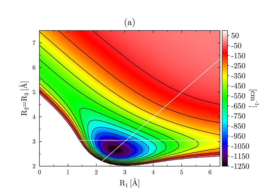
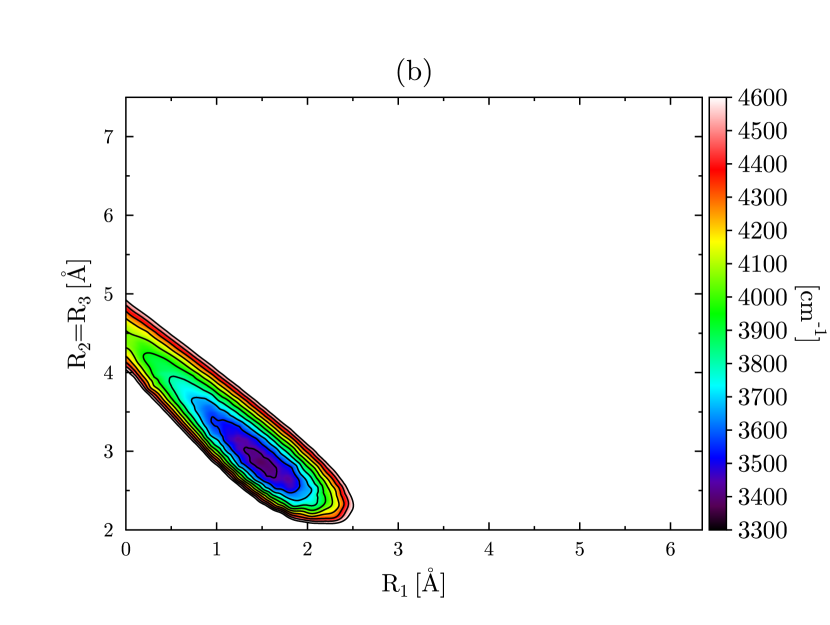
Figure 3: (Color online) Two-dimensional contour plots of the quartet ground state $1{\,}\tensor{*}[^{4}]{\mathrm{B}}{{}_{1}}$ in (a) and the first quartet excited state $1{\,}\tensor{*}[^{4}]{\mathrm{A}}{{}_{2}}$ in (b) PESs in the subspace $R_{1}$ and $R_{2}=R_{3}$ of perimetric coordinates, i.e. along one space diagonal surface in Fig. 2 (c). The space diagonal (i.e. $D_{3h}$ configurations) corresponds to the diagonal line shown in white, while the horizontal line (both in (a)) represents the special one-dimensional $C_{2v}$-cut for $R_{23}=$6.094\text{\,}\mathrm{\SIUnitSymbolAngstrom}$$. The wavy character in (b) is due to the underlying spline interpolation of the corresponding ab-initio data.

To get an idea of the system’s physics, in particular the occurring coupling and crossing effects, we start with analyzing special cuts through the PESs of both doublet and quartet manifolds. For this we restrict our investigations to the $C_{2v}$ subspace since it turns out that all equilibrium structures show at least $C_{2v}$ symmetry. Therefore we are labeling the resulting electronic states according to the irreducible representations (IRREPs) of this point group. Given the choice of coordinates shown in Fig. 2 (a), $\mathrm{A}_{1}$ and $\mathrm{B}_{1}$ states are symmetric, and $A_{2}$ and $B_{2}$ states are antisymmetric with respect to reflection of the electronic coordinates at the molecular plane. Figure 3 gives a first impression of the topology of the potential energy landscapes for the quartet ground state ($1{\,}\tensor{*}[^{4}]{\mathrm{B}}{{}_{1}}$) and the first excited quartet state ($1{\,}\tensor{*}[^{4}]{\mathrm{A}}{{}_{2}}$) in terms of two-dimensional cuts for $C_{2v}$-symmetric nuclear configurations. These correspond to one of the space diagonal surfaces shown in Fig. 2 (c). The quartet ground state ($1{\,}\tensor{*}[^{4}]{\mathrm{B}}{{}_{1}}$) in Fig. 3 (a) is well isolated from excited quartet states (i.e. crossings with other states only appear at energies high above the minimum and the dissociation limit of this state) with the global minimum occurring at equilateral triangular ($D_{3h}$) geometry Soldán (2010). At a symmetric linear geometry (for this cut at $R_{1}=0$) we obtain a saddle point marking the transition to the inverted structure. Moreover, we note that the PES of the $1{\,}\tensor{*}[^{4}]{\mathrm{B}}{{}_{1}}$ is rather shallow. These properties have also been pointed out by Soldán in his work concerning the quartet ground state of Rb3 in Ref. Soldán (2010). Figure 3 (b) shows the first excited quartet state ($1{\,}\tensor{*}[^{4}]{\mathrm{A}}{{}_{2}}$ in $C_{2v}$) with the global minimum occurring at isosceles triangular (i.e. $C_{2v}$) geometry. This is due to the JT effect forming a twofold degenerate $\mathrm{E}^{\prime\prime}$ state (with $1{\,}\tensor{*}[^{4}]{\mathrm{B}}{{}_{2}}$) at $D_{3h}$ geometries (this will be discussed in more detail in Sec. III.3). This PES rises significantly steeper than the shallow quartet ground state PES.

The presence of (pseudo) Jahn-Teller interactions can be also observed from one-dimensional scans along the $D_{3h}$ subspace, i.e. along the diagonal shown in white in Fig. 3 (a). The resulting potential energy curves (PECs) are shown in Fig. 4 in the space of internal coordinates ($R_{12}=R_{23}=R_{13}$).

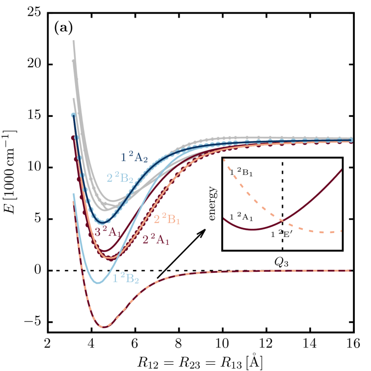
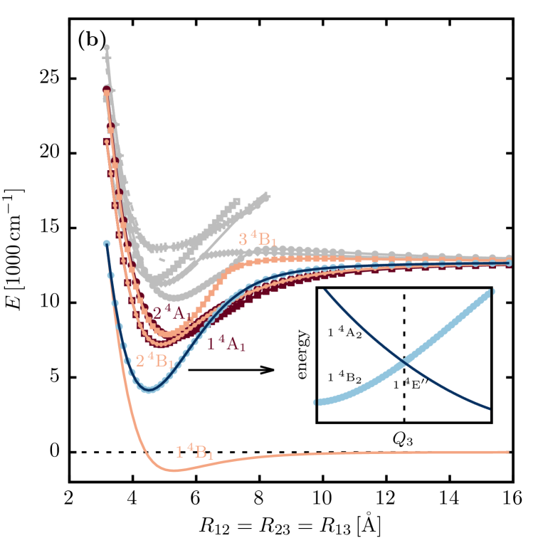
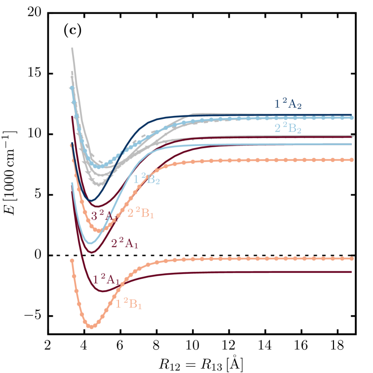
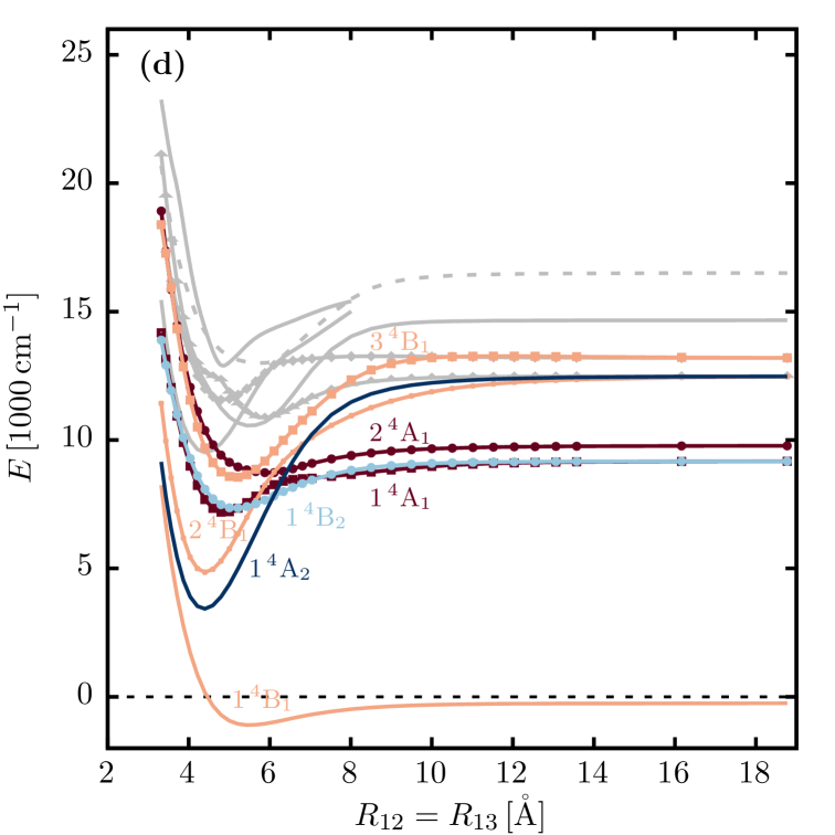
Figure 4: (Color online) Upper panel: One-dimensional cut through the potential energy surfaces (PESs) along the space diagonal in the perimetric coordinate space shown Fig. 2 (c) and in terms of the diagonal shown Fig. 3 (a) (i.e. $D_{3h}$ scan maintaining the equilateral triangular configuration). Doublet states are shown in (a) and quartet states in (b), respectively. The low-lying states discussed in the text are highlighted, the presence of further states is indicated by the gray lines. Lower panel: One-dimensional cut through the PESs along one special direction on one space diagonal surface shown in Fig. 2 (c). This $C_{2v}$ scan corresponds to a fixed distance $R_{23}=R_{e}(a{\,}^{3}\Sigma_{u})=$6.094\text{\,}\mathrm{\SIUnitSymbolAngstrom}$$. Doublets are shown in (c) and quartets in (d), respectively.

Equilateral triangular configurations of homonuclear triatomics display $D_{3h}$ symmetry and allow for two-fold degenerate, so called $\mathrm{E}$ terms (cf. Tab. LABEL:S-tab:D3h in the supplementary material Sup ). According to the Jahn-Teller theorem Bersuker (2001); Domcke et al. (2006); Thapaliya et al. (2015); Barckholtz and Miller (1998); Poluyanov and Domcke (2008); Rocha and Varandas (2016), the PES of at least one of these degenerate states has no extremum at this high-symmetry point. Thus, the system lowers its symmetry to lift the degeneracy, here branching off into $\mathrm{A}_{1}+\mathrm{B}_{1}$ states for $\mathrm{E}^{\prime}$ or into $\mathrm{B}_{2}+\mathrm{A}_{2}$ states for $\mathrm{E}^{\prime\prime}$, respectively. This is accompanied by an energy lowering and the formation of a COIN at the point of degeneracy. This is also indicated by the insets shown in Fig. 4. Potential energy curves which are degenerate over the whole range shown in Fig. 4 are actually one-dimensional COIN seams in the three-dimensional configuration space.

The doublet ground states of alkali trimers show their global minimum at obtuse isosceles triangular geometries due to the JT effect (studied theoretically for Li3 in Refs. Martins et al. (1983); Thompson et al. (1985), for Na3 in Refs. Martins et al. (1983); Martin and Davidson (1978); Thompson et al. (1985); Cocchini et al. (1988), for K3 in Refs. Martins et al. (1983); Thompson et al. (1985); Hauser et al. (2008); Mukherjee and Adhikari (2014) and for Rb3 in Refs. Hauser et al. (2010b, 2009); Hauser (2009)). This finding is also illustrated by the corresponding PECs in Fig. 4 (a) (and by the alternative one-dimensional cuts in Fig. LABEL:S-fig:JT-scans-QD in the supplementary material Sup ). A further peculiarity – well-known as the pseudo Jahn-Teller (PJT) effect – is formed, e.g., by the triple of states $\{2{\,}\tensor{*}[^{2}]{\mathrm{A}}{{}_{1}},2{\,}\tensor{*}[^{2}]{\mathrm{B}}{{}_{1}},3{\,}\tensor{*}[^{2}]{\mathrm{A}}{{}_{1}}\}$, where $2{\,}\tensor{*}[^{2}]{\mathrm{A}}{{}_{1}}$ and $2{\,}\tensor{*}[^{2}]{\mathrm{B}}{{}_{1}}$ are degenerate components of the $2{\,}\tensor{*}[^{2}]{\mathrm{E}}{{}^{\prime}}$ term (for $D_{3h}$ configurations) and the $3{\,}\tensor{*}[^{2}]{\mathrm{A}}{{}_{1}}$ state is nearby in energy (near degeneracy) – cf. Fig. 4 (a) and Fig. LABEL:S-fig:JT-scans-QD. Consequently, all three states can mix for $C_{2v}$ configurations which is described within the theory of pseudo JT-coupling (cf. e.g. Refs. Liu et al. (2010); Bersuker (2013)). It follows that due to the third state which is close in energy the COIN seam of the doubly degenerate JT state at high-symmetry geometries vanishes. Only at a single point in the $D_{3h}$ subspace all three states become degenerate forming a triply degenerate COIN point Cocchini et al. (1988). This intersection is analogous to the JT one, but it is not required by symmetry (accidental degeneracy). All of this is essential to fully understand the well-known experimentally observed $\mathrm{B}$ band in alkali metal triatomics Bersuker (2001).

In contrast to the doublet ground state, the quartet ground state is free of JT distortions with its global minimum at $D_{3h}$ configuration. The first pair of excited quartet states, however, is degenerate along a one-dimensional COIN seam in the $D_{3h}$ configuration space, and spans a $1{\,}\tensor{*}[^{4}]{\mathrm{E}}{{}^{\prime\prime}}$ term, which splits into $1{\,}\tensor{*}[^{4}]{\mathrm{A}}{{}_{2}}$ and $1{\,}\tensor{*}[^{4}]{\mathrm{B}}{{}_{2}}$ states when the symmetry is lowered. Besides those states which are exactly degenerate, there are also a number of nearly degenerate states. In particular, there are quadruple interactions Hauser (2009) present within the subset $\mathcal{Q}$ of quartet states

$$\mathcal{Q} =\{1{\,}\tensor{*}[^{4}]{\mathrm{A}}{{}_{1}},2{\,}\tensor{*}[^{4}]{\mathrm{A}}{{}_{1}},2{\,}\tensor{*}[^{4}]{\mathrm{B}}{{}_{1}},3{\,}\tensor{*}[^{4}]{\mathrm{B}}{{}_{1}}\}\,.$$ (18)

This peculiarity can be seen in Fig. 4 (b) (and Fig. LABEL:S-fig:JT-scans-QD (b) in the supplementary material Sup ), where those states are almost degenerate in a region reaching from $\approx$5.0\text{\,}\mathrm{\SIUnitSymbolAngstrom}$$ to $\approx$7.0\text{\,}\mathrm{\SIUnitSymbolAngstrom}$$. More details on all JT and PJT pairs within this energy range can be found in the supplementary material Sup in Tab. LABEL:S-tab:PJTStates.

The other one-dimensional cut indicated in Fig. 3 (a) corresponds to a collision trajectory between a Rb2 molecule and a Rb atom. For this cut, we fixed the distance $R_{23}$ to the equilibrium distance of the lowest triplet state ($a{\,}^{3}\Sigma_{u}$) of Rb2. The resulting cuts in Figs. 4 (c) and (d) give a first impression of the states possibly involved in a PA 1 scheme. Moreover, this graph shows one dimension of the 2D branching space (formally spanned by $Q_{2}$ and $Q_{3}$, cf. Sec. II.2) where the degeneracies from high-symmetry configurations (here found at the point $R_{12}=R_{13}=R_{23}=$6.094\text{\,}\mathrm{\SIUnitSymbolAngstrom}$$) are lifted. This gives a notion of the topology of the full 3D potential energy landscape. The density of states increases for higher energies for both doublet and quartet manifolds and decreases the chance for finding sufficiently long-lived target states for PA experiments. Therefore and due to the fact that the doublet ground state has a rather complex behavior due to JT distortions we focus on quartet states.

Linear configurations of the trimer system are subject to Renner-Teller (RT) or combined PJT plus RT interactions. A detailed analysis of this, however, is beyond the scope of the present work. Nevertheless, a comment can be found in the supplementary material Sup .

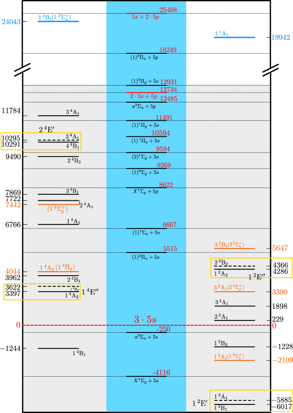
Figure 5: (Color online) Energy level diagram of the extremal points of doublet (right) and quartet (left) states of Rb3 optimized at MRCI(ECP+CPP)/UET15 level of theory. The dissociation asymptotes into Rb2+Rb (with the corresponding equilibrium energies of the Rb2 states) or Rb+Rb+Rb are shown in the area highlighted in blue. Levels given in black belong to triangular equilibrium configurations (i.e. $D_{3h}$ or $C_{2v}$ symmetry) while levels given in orange represent linear equilibrium configurations (all of them $D_{\infty h}$ symmetry). Yellow boxes mark Jahn-Teller states, where the respective dashed lines correspond to saddle points showing isosceles triangular geometry. The ionized $\mathrm{Rb}_{3}^{+}$ states are shown at the top in terms of blue energy levels. All energies are given relative to the free atom-atom-atom limit (i.e. $3\cdot\ce{Rb}\left[5s\right]$).

II.4 Equilibrium States

A systematic overview of the energy levels of all doublet and quartet states of Rb3 considered in this work is given in Fig. 5. All energy levels refer to the electronic energy at the equilibrium geometry. For finding the equilibrium states we started from high-symmetry configurations ($D_{3h}$) and proceeded to geometries of lower symmetry ($C_{2v}$). Our analysis did not show any evidence for equilibrium structures of even lower symmetry, i.e. $C_{s}$. We determined all equilibrium states and their electronic term energies in the energy region up to the $5s+2\cdot 5p$ asymptote. The energies of the Rb2+Rb or Rb+Rb+Rb dissociation asymptotes are given in the middle panel. The assignment of the trimer states to the Rb2+Rb asymptotes is in general only unique for the quartet ground state $1{\,}\tensor{*}[^{4}]{\mathrm{B}}{{}_{1}}$ dissociating into $a{\,}\tensor{*}[^{3}]{\Sigma}{{}_{u}}+5s$. For one-dimensional $C_{2v}$ cuts as shown in Fig. 4 (c) and (d) we obtain a unique assignment for all quartet states and some doublet states as well. However, in the general case, for both doublet and quartet states, all Rb2+Rb asymptotes correlating with the respective trimer state symmetry are possible dissociation channels. Most of the excited states correlate to the $2\cdot 5s+5p$ asymptote. Merely the highly excited quartet states $2{\,}\tensor{*}[^{4}]{\mathrm{B}}{{}_{2}}$, $3{\,}\tensor{*}[^{4}]{\mathrm{B}}{{}_{2}}$ and $4{\,}\tensor{*}[^{4}]{\mathrm{A}}{{}_{1}}$ correspond to the $5s+2\cdot 5p$ asymptote and thus to the $(1)\,\tensor{*}[^{3}]{\Pi}{{}_{u}}+5p$ dissociation limit. The lowest doublet JT manifold $1{\,}\tensor{*}[^{2}]{\mathrm{E}}{{}^{\prime}}=1{\,}\tensor{*}[^{2}]{\mathrm{A}}{{}_{1}}+1{\,}\tensor{*}[^{2}]{\mathrm{B}}{{}_{1}}$ dissociates either to $X{\,}\tensor{*}[^{1}]{\Sigma}{{}_{g}}+5s$ or to $a{\,}\tensor{*}[^{3}]{\Sigma}{{}_{u}}+5s$. The remaining doublet states correspond to Rb2+Rb asymptotes below the $2\cdot 5s+5p$ asymptote where both singlet and triplet Rb2 states are possible. Finally, the top panel of Fig. 5 also shows the ionized states of Rb3+ appearing in either singlet or triplet configuration. This could be useful if a REMPI Wolf et al. (2017) scheme is used for the detection of previously generated Rb3 species. All these results are listed in Tab. 2 (for triangular geometries) and in Tab. 3 (for linear configurations) together with their corresponding harmonic vibrational frequencies $\tilde{\nu}$.

Table 2: Synopsis of triangular ($C_{2v}$ and $D_{3h}$) doublet and quartet (ground and excited) states of Rb3 as well as the singlet state of Rb3+ computed at MRCI(ECP+CPP)/UET15 level of theory. Equilibrium structures are given in terms of the internal coordinates (perimetric coordinates) introduced in Fig. 2 and all corresponding energies ($E_{\text{rel}}$) are given relative to the $(3\cdot 5s)$–asymptote calculated at the same level of theory. The states are labelled according to the $C_{2v}$ IRREPs while the corresponding assignment to $D_{3h}$ symmetry is given in parenthesis. This complements the results of the energy level diagram of Fig. 5.

State ($D_{3h}$)	$R_{12},R_{23},R_{13}\,[\mathrm{\mathring{A}}]$	Geometry	$E_{\text{rel}}\,[\mathrm{cm}^{-1}]$	$\tilde{\nu}_{D_{3h}}\,[\mathrm{cm}^{-1}]$	$\tilde{\nu}_{C_{2v}}\,[\mathrm{cm}^{-1}]$1	$\tilde{\nu}_{C_{s}}\,[\mathrm{cm}^{-1}]$1
	$(R_{1},R_{2},R_{3})$
$1{\,}\tensor{*}[^{4}]{\mathrm{B}}{{}_{1}}$ ($1{\,}\tensor{*}[^{4}]{\mathrm{A}}{{}^{\prime}_{2}}$)	$5.311,5.311,5.311$	$D_{3h}$	$-1244$	$23.8$	$23.6$	$23.6$
	$(2.656,2.656,2.656)$
$1{\,}\tensor{*}[^{4}]{\mathrm{A}}{{}_{2}}$ ($1{\,}\tensor{*}[^{4}]{\mathrm{E}}{{}^{\prime\prime}}$)	$4.368,5.700,4.368$	$C_{2v}$	3397	$50.2$	$17.2$	$35.8$
	$(1.518,2.850,2.850)$
$2{\,}\tensor{*}[^{4}]{\mathrm{B}}{{}_{1}}$ ($1{\,}\tensor{*}[^{4}]{\mathrm{E}}{{}^{\prime}}$)	$4.442,8.179,4.442$	$C_{2v}$	3962	$40.3$	$9.6$	$40.4$
	$(0.352,4.090,4.090)$
$1{\,}\tensor{*}[^{4}]{\mathrm{A}}{{}_{1}}$ ($1{\,}\tensor{*}[^{4}]{\mathrm{E}}{{}^{\prime}}$)	$4.993,8.076,4.993$	$C_{2v}$	6766	$32.8$	$9.8$	$50.7$
	$(0.955,4.038,4.038)$
$2{\,}\tensor{*}[^{4}]{\mathrm{A}}{{}_{1}}$ ($1{\,}\tensor{*}[^{4}]{\mathrm{A}}{{}^{\prime}_{1}}$)	$5.325,5.325,5.325$	$D_{3h}$	7722	$32.0$	$83.9$	$83.9$
	$(2.663,2.663,2.663)$
$3{\,}\tensor{*}[^{4}]{\mathrm{B}}{{}_{1}}$ ($2{\,}\tensor{*}[^{4}]{\mathrm{A}}{{}^{\prime}_{2}}$)	$5.084,5.084,5.084$	$D_{3h}$	7869	$43.0$	$58.2$	$58.2$
	$(2.542,2.542,2.542)$
$2{\,}\tensor{*}[^{4}]{\mathrm{B}}{{}_{2}}$ ($2{\,}\tensor{*}[^{4}]{\mathrm{E}}{{}^{\prime\prime}}$)	$4.443,6.217,4.443$	$C_{2v}$	9490	$52.0$	$42.7$	$41.3$
	$(1.335,3.109,3.109)$
$4{\,}\tensor{*}[^{4}]{\mathrm{B}}{{}_{1}}$ ($2{\,}\tensor{*}[^{4}]{\mathrm{E}}{{}^{\prime}}$)	$5.283,5.337,5.283$	$C_{2v}$	10291	$31.5$	$37.7$	$39.0$
	$(2.615,2.669,2.669)$
$3{\,}\tensor{*}[^{4}]{\mathrm{A}}{{}_{1}}$ (upper) ($2{\,}\tensor{*}[^{4}]{\mathrm{E}}{{}^{\prime}}$)	$4.687,7.226,4.687$	$C_{2v}$	11784	$41.5$	$28.2$	$27.5$
	$(1.074,3.613,3.613)$
$1{\,}\tensor{*}[^{2}]{\mathrm{B}}{{}_{1}}$ ($1{\,}\tensor{*}[^{2}]{\mathrm{E}}{{}^{\prime}}$)	$4.379,5.393,4.379$	$C_{2v}$	-6017	$53.1$	$20.6$	$33.3$
	$(1.682,2.697,2.697)$
$1{\,}\tensor{*}[^{2}]{\mathrm{B}}{{}_{2}}$ ($1{\,}\tensor{*}[^{2}]{\mathrm{A}}{{}^{\prime\prime}_{2}}$)	$4.276,4.285,4.276$	$C_{2v}$	-1228	$60.9$	$43.9$	$44.1$
	$(2.134,2.143,2.143)$
$2{\,}\tensor{*}[^{2}]{\mathrm{A}}{{}_{1}}$ ($2{\,}\tensor{*}[^{2}]{\mathrm{E}}{{}^{\prime}}$)	$4.398,6.073,4.398$	$C_{2v}$	229	$50.4$	$26.7$	$42.1$
	$(1.361,3.037,3.037)$
$3{\,}\tensor{*}[^{2}]{\mathrm{A}}{{}_{1}}$ ($1{\,}\tensor{*}[^{2}]{\mathrm{A}}{{}^{\prime}_{1}}$)	$4.557,4.557,4.557$	$D_{3h}$	1898	$51.9$	$100.6$	$100.6$
	$(2.279,2.279,2.279)$
$1{\,}\tensor{*}[^{2}]{\mathrm{A}}{{}_{2}}$ ($1{\,}\tensor{*}[^{2}]{\mathrm{E}}{{}^{\prime\prime}}$)	$4.337,5.132,4.337$	$C_{2v}$	4286	$52.9$	$23.7$	$30.2$
	$(1.771,2.566,2.566)$
$1{\,}\tensor{*}[^{1}]{\mathrm{A}}{{}_{1}}$ (${\,}\tensor{*}[^{1}]{\mathrm{A}}{{}^{\prime}_{1}}$)	$4.610,4.610,4.610$	$D_{3h}$	19942	$53.2$	$36.6$	$36.5$
	$(2.305,2.305,2.305)$

Table 3: Synopsis of linear ($D_{\infty h}$) doublet and quartet (ground and excited) states of Rb3 as well as the triplet state of Rb3+ computed at MRCI(ECP+CPP)/UET15 level of theory. Equilibrium structures are given in terms of the internal coordinates (perimetric coordinates) introduced in Fig. 2 and all corresponding energies ($E_{\text{rel}}$) are given relative to the $(3\cdot 5s)$–asymptote calculated at the same level of theory. The states are labelled according to the $C_{2v}$ IRREPs while the corresponding assignment to $D_{\infty h}$ symmetry is given in parenthesis. This complements the results of the energy level diagram of Fig. 5.

State ($D_{\infty h}$)	$R_{12},R_{23},R_{13}\,[\mathrm{\mathring{A}}]$	$E_{\text{rel}}\,[\mathrm{cm}^{-1}]$	$\tilde{\nu}_{\text{symm}}\,[\mathrm{cm}^{-1}]$	$\tilde{\nu}_{\text{asymm}}\,[\mathrm{cm}^{-1}]$	$\tilde{\nu}_{\text{bending}_{1}}\,[\mathrm{cm}^{-1}]$	$\tilde{\nu}_{\text{bending}_{2}}\,[\mathrm{cm}^{-1}]$
	$(R_{1},R_{2},R_{3})$
$1{\,}\tensor{*}[^{4}]{\mathrm{A}}{{}_{2}}+2{\,}\tensor{*}[^{4}]{\mathrm{B}}{{}_{1}}$($1{\,}\tensor{*}[^{4}]{\Pi}{{}_{g}}$)	$4.435,8.869,4.435$	4044	$33.7$	$41.7$	$236.8$	$84.7$
	$(0.000,4.435,4.435)$
$2{\,}\tensor{*}[^{4}]{\mathrm{A}}{{}_{1}}$ ($1{\,}\tensor{*}[^{4}]{\Sigma}{{}^{+}_{g}}$)	$4.937,9.874,4.937$	7442	$398.2$	$48.9$	$282.6$	$282.6$
	$(0.000,4.937,4.937)$
$1{\,}\tensor{*}[^{2}]{\mathrm{A}}{{}_{1}}$ ($1{\,}\tensor{*}[^{2}]{\Sigma}{{}^{+}_{g}}$)	$4.795,9.590,4.795$	-2109	$24.9$	$60.8$	$4.1$	$4.1$
	$(0.000,4.795,4.795)$
$3{\,}\tensor{*}[^{2}]{\mathrm{A}}{{}_{1}}$ ($2{\,}\tensor{*}[^{2}]{\Sigma}{{}^{+}_{g}}$)3	$4.440,8.880,4.440$	3390	$405.9$	$46.9$	$313.8$	$350.3$
	$(0.000,4.440,4.440)$
$3{\,}\tensor{*}[^{2}]{\mathrm{B}}{{}_{1}}$ ($2{\,}\tensor{*}[^{2}]{\Sigma}{{}^{+}_{u}}$)	$4.930,9.860,4.930$	5647	$27.7$	$48.4$	$169.6$	$169.6$
	$(0.000,4.930,4.930)$
$1{\,}\tensor{*}[^{3}]{\mathrm{B}}{{}_{1}}$ ($\tensor{*}[^{3}]{\Sigma}{{}^{+}_{u}}$)	$4.875,9.749,4.875$	24043	$30.3$	$49.7$	$6.3$	$6.3$
	$(0.000,4.875,4.875)$

Our results are in good agreement with previous theoretical studies of Rb3. For the quartet ground state Soldán Soldán (2010) found equilateral bond distances $b$ with $b=$5.450\text{\,}\mathrm{\SIUnitSymbolAngstrom}$$, using the RHF-RCCSD(T) approach with a [16s13p8d5f3g] basis and the small-core ECP from Ref. Lim et al. (2005) (ECP28MDF). The energy of the minimum was determined at $E_{\text{min}}=-1071\,\mathrm{cm}^{-1}$. Hauser et al. Hauser et al. (2010a); Hauser and Ernst (2011) found for the equilateral bond distances $b=$5.500\text{\,}\mathrm{\SIUnitSymbolAngstrom}$$ with corresponding energy $E_{\text{min}}=-939\,\mathrm{cm}^{-1}$ and harmonic frequencies $\{\tilde{\nu}_{D_{3h}},\tilde{\nu}_{C_{2v}},\tilde{\nu}_{C_{s}}\}=\{18,21,21\}\,\mathrm{cm}^{-1}$ using RHF-RCCSD(T) with the ECP28MDF small-core ECP and the corresponding original basis set augmented by a $(1s,1p,1d)$ set of diffuse functions. In comparison, our computations give a binding energy of $-1244\,\mathrm{cm}^{-1}$, equilateral bond distances of $5.311\,$\mathrm{\SIUnitSymbolAngstrom}$$ and vibrational frequencies of $\{\tilde{\nu}_{D_{3h}},\tilde{\nu}_{C_{2v}},\tilde{\nu}_{C_{s}}\}=\{23.8,23.6,23.6\}\,\mathrm{cm}^{-1}$. In case of the doublet ground state Hauser et al. Hauser et al. (2010a, b) obtained bond distances with $R_{12}=R_{13}=$4.387\text{\,}\mathrm{\SIUnitSymbolAngstrom}$$, $R_{23}=$5.575\text{\,}\mathrm{\SIUnitSymbolAngstrom}$$ and the equilibrium energy $E_{\text{min}}=-5321\,\mathrm{cm}^{-1}$ using RHF-UCCSD(T), small-core ECP and a [14s,11p,6d,3f,1g] uncontracted even-tempered basis set derived from the ECP28MDF basis. Our calculations result in bond distances with $R_{12}=R_{13}=$4.379\text{\,}\mathrm{\SIUnitSymbolAngstrom}$$ and $R_{23}=$5.393\text{\,}\mathrm{\SIUnitSymbolAngstrom}$$ with a corresponding binding energy of $-6017\,\mathrm{cm}^{-1}$. Moreover, we can extract the vertical transition energy from the quartet ground state to the high-spin $2{\,}\tensor{*}[^{4}]{\mathrm{E}}{{}^{\prime}}$ manifold from Fig. 5 and Tab. 2 and compare the result with the one calculated by Hauser et al. Hauser et al. (2010a); Hauser and Ernst (2011) using a modified version of CASPT2 (referred to as RS2C in Molpro), the same small-core ECP as well as the same basis set as described before. Our result is $E_{2{\,}\tensor{*}[^{4}]{\mathrm{E}}{{}^{\prime}}\leftarrow 1{\,}\tensor{*}[^{4}]{\mathrm{A}}{{}_{2}^{\prime}}}=11535\,\mathrm{cm}^{-1}$ compared to the result $11530\,\mathrm{cm}^{-1}$ of Hauser et al. The corresponding experimental value Nagl et al. (2008a); Giese et al. (2011) is $11510\,\mathrm{cm}^{-1}$ referring to the lowest-energy maximum band of the measured band spectra applying laser-induced fluorescence (LIF) spectroscopy to Rb3 clusters formed on helium nanodroplets.

In the supplementary material Sup in Tabs. LABEL:S-tab:Rb3statesTriangularSupp and LABEL:S-tab:Rb3statesLinearSupp and Fig. LABEL:S-fig:termschemeSupp we are providing a more detailed overview on all states, i.e. by including saddle points, obtained within the energy range up to the $5s+2\cdot 5p$ asymptote. Some of the saddle points define the barrier heights between minima on PESs. This becomes important for analyzing the JT effect.

II.5 Survey of Spin-Orbit Coupling Effects

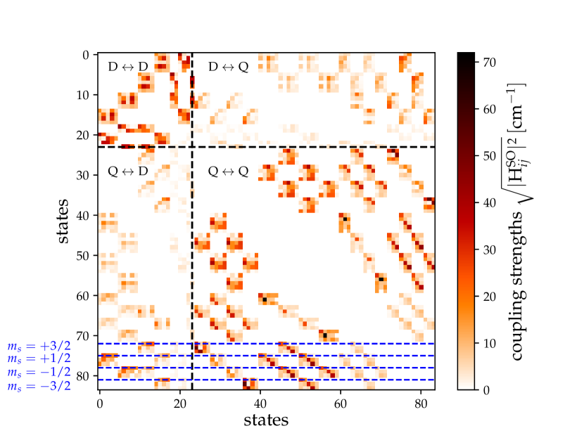
Figure 6: (Color online) Heat-map representation of the absolute values of the spin-orbit matrix $\sqrt{|\hat{H}^{\text{SO}}_{ij}|^{2}}$ (without diagonal elements). The Rb3 geometry was fixed to the equilibrium configuration of the first excited quartet state $1{\,}\tensor{*}[^{4}]{\mathrm{A}}{{}_{2}}$ (see Tab. 2). The partitioning separates doublet-doublet (D$\leftrightarrow$D), quartet-quartet (Q$\leftrightarrow$Q) and quartet-doublet (Q$\leftrightarrow$D) couplings. The dashed blue lines mark the rows where the four components corresponding to the $1{\,}\tensor{*}[^{4}]{\mathrm{A}}{{}_{2}}$ state are found in the SO-matrix. The SO matrix is sorted according to IRREPs ($C_{2v}$) in the sequence ($\mathrm{A}_{1}$/$\mathrm{B}_{1}$/$\mathrm{B}_{2}$/$\mathrm{A}_{2}$) where each of them (in zeroth order basis) are ordered with respect to increasing energy and are accordingly combined with the $m_{s}$ spin function starting from $m_{s}=+\nicefrac{{1}}{{2}}$ to $m_{s}=-\nicefrac{{1}}{{2}}$ for doublets and $m_{s}=+\nicefrac{{3}}{{2}}$ to $m_{s}=-\nicefrac{{3}}{{2}}$ for quartets. This is a complete representation with respect to the energetically lowest 12 doublet (5/4/2/1) and 15 quartet states (4/5/3/3) leading to the $84\times 84$ SO-matrix.

Spin-orbit coupling (SOC) is still a comparatively weak effect for Rb (the SOC induced splitting of the atomic $\tensor{*}[^{2}]{\mathrm{P}}{}$ state is $\approx 240\,\mathrm{cm}^{-1}$) and the classification of states in terms of their total spin, as in the previous sections, is justified. Nevertheless, in particular in the vicinity of degeneracies, SOC can lead to a mixing of states of the same or of different spin. To get an idea of the importance of this phenomenon we have investigated the size of the couplings for selected nuclear configurations at the MRCI(ECP+CPP)/UET15 level of theory using the ECP-LS technique for the corresponding large-core pseudopotential. All important details about the computation of the corresponding spin-orbit matrix based on a pseudopotential approach can be found, e.g., in Refs. Silberbach et al. (1986); Dolg (2000). The computations included 15 quartet (4/5/3/3) and 12 doublet (5/4/2/1) states, according to the Molpro specific ordering of the IRREPs ($\mathrm{A}_{1}$/$\mathrm{B}_{1}$/$\mathrm{B}_{2}$/$\mathrm{A}_{2}$). That is, in total a $84\times 84$ SO-matrix is set up and diagonalized.

To get a qualitative overview we show in Fig. 6 the absolute values of the SO-matrix $|\hat{H}^{\text{SO}}_{ij}|$ at the equilibrium geometry of the first excited quartet state $1{\,}\tensor{*}[^{4}]{\mathrm{A}}{{}_{2}}$ as a heat-map representation. It should look similar for comparable geometrical configurations. The main contributions come from doublet-doublet ($\mathrm{D}\leftrightarrow\mathrm{D}$), respectively quartet-quartet ($\mathrm{Q}\leftrightarrow\mathrm{Q}$) couplings. However, there are also non-vanishing couplings between quartet and doublet states ($\mathrm{Q}\leftrightarrow\mathrm{D}$ and vice versa). The corresponding selection rules (for $C_{2v}$ configurations), deduced from group theory, allow for $\Delta S=0,\pm 1$ and couplings between all combinations of IRREPs except the same (a detailed derivation is given in the supplementary material Sup ).

The explicit values for resulting shifts and zero-field splittings (i.e. the lifting of degenerate states in the absence of a magnetic field) are given in Tabs. LABEL:S-tab:SOCRb3Q to LABEL:S-tab:SOCRb3DLin in the supplementary material Sup for the equilibrium states listed in Tabs. 2 and 3 together with the corresponding most dominantly coupling states. Typical coupling strengths amount to 20 to 70 $\mathrm{cm}^{-1}$, as shown in Fig. 6, but the resulting energy shifts and zero-field splittings are much smaller. For instance the quartet ground state splits into the two states $\mathrm{E}_{1/2}$ and $\mathrm{E}_{3/2}$ of the $D_{3h}$ spin double group Hauser et al. (2010a), but the corresponding zero-field splitting is less than $0.1\,\mathrm{cm}^{-1}$ and the energy lowering induced by the SOC is less than $0.2\,\mathrm{cm}^{-1}$. The same observation holds for the first excited quartet state $1{\,}\tensor{*}[^{4}]{\mathrm{A}}{{}_{2}}$ for which these SOC effects are again smaller than $1\,\mathrm{cm}^{-1}$. The reason for these small values lies in the effective quenching of the orbital angular momentum in triangular geometries and in the energy separation to other states. For highly symmetric configurations, in particular for linear geometries and in the presence of spatial degeneracies, the effects become larger, e.g. for the $1{\,}\tensor{*}[^{4}]{\Pi}{{}_{g}}$ state, for which splittings and energy shifts of up to 200 $\mathrm{cm}^{-1}$ are computed.

The strength of SOC, in particular between the quartet ground state $1{\,}\tensor{*}[^{4}]{\mathrm{B}}{{}_{1}}$ and the first excited quartet state $1{\,}\tensor{*}[^{4}]{\mathrm{A}}{{}_{2}}$, decays with respect to distortions from equilateral triangular geometries. Only in the limit of dissociation into both Rb2$+$Rb and $3\cdot\ce{Rb}$ SOC effects become larger, since Rb2 always has a well-defined $C_{\infty}$ axis. To summarize, we do not expect significant SOC induced mixing of the states in the vicinity of equilibrium geometries, in particular for the low-lying states $1{\,}\tensor{*}[^{4}]{\mathrm{B}}{{}_{1}}$ and $1{\,}\tensor{*}[^{4}]{\mathrm{A}}{{}_{2}}$.

III Identifying Appropriate States for Photoassociation

III.1 Configuration Space Survey

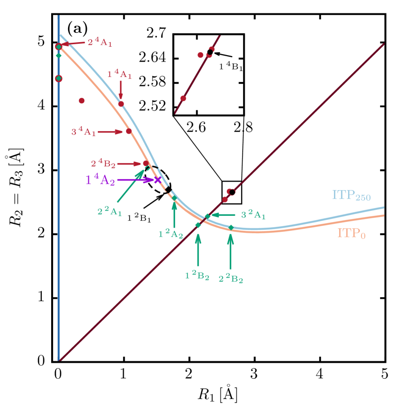
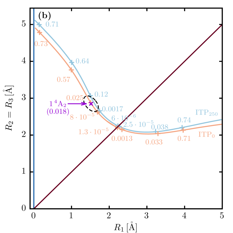
Figure 7: (Color online) Inner-turning point (ITP) locations and locations of equilibrium geometries in the configuration space of perimetric coordinates. (a) Since all equilibrium geometries show at least $C_{2v}$ symmetry the configuration space survey can be restricted to one of the space diagonal surfaces shown in Fig. 2 (c). Inner turning points (ITPs) on the quartet ground state PES with respect to either the $\ce{Rb2}+\ce{Rb}$ or $3\cdot\ce{Rb}$ dissociation scenarios are given in light blue for the first one and in light red for the latter. States lying close to this lines are promising candidates for showing good Franck-Condon factors. Here we focus on the $1{\,}\tensor{*}[^{4}]{\mathrm{A}}{{}_{2}}$ state highlighted in purple. The numbers given in (b) along both ITP lines represent the electronic dipole transition strengths (in units of $[\mathrm{D}^{2}]$) between the quartet ground state and this $1{\,}\tensor{*}[^{4}]{\mathrm{A}}{{}_{2}}$ state at the corrsponding ITP locations. Note that the numbers given in (b) do not correlate with the equilibrium geometries depicted in (a). The transition dipole strength at the equilibrium geometry of the first excited quartet state amounts to $0.018\,\mathrm{D}^{2}$. The ellipses shown in (a) and (b) give an estimate of the size of the vibrational ground state wavefunction for the $1{\,}\tensor{*}[^{4}]{\mathrm{A}}{{}_{2}}$ state.

For the realization of the trimer PA processes, non-vanishing Franck-Condon factors are required, i.e. a significant overlap of the nuclear scattering wavefunction of Rb2$+$Rb or $3\cdot\ce{Rb}$ collisions and the molecular trimer vibrational wavefunction of the excited state. In this work we are mostly interested in producing deeply bound trimers close to the vibrational ground state for reasons of increased stability, lifetime and simplicity. In fact, as we will show in the following, it turns out that the equilibrium geometries of a number of excited states are in close proximity to the inner-turning points (ITPs) of the scattering wavefunction. Since the scattering wavefunction typically exhibits a local maximum at the ITP this suggests that favourable Franck-Condon factors might be found for photoassociating excited trimers in their equilibrium geometry. For trimers, the ITPs are actually 2D surfaces in the configuration space. They correspond to those points where the quartet ground state PES equals to the energy of the scattering state. For the case of Rb2$+$Rb this energy is given by the negative binding energy of the $a{\,}\tensor{*}[^{3}]{\Sigma}{{}_{u}}$ state of Rb2, i.e. $\approx-250\,\mathrm{cm}^{-1}$, and for the case of $3\cdot\ce{Rb}$ the energy is approximately zero. Again, note that PA2 at short distances is expected to be rather unlikely due to the effective repulsive barrier in the short-range of the three-body potential, cf. Ref. Wang et al. (2012). Nevertheless, at large distances PA2 should be possible. The feasibility for PA1 is shown in Ref. Pérez-Ríos et al. (2015). The locations of the ITPs (i.e. $\mathrm{ITP}_{250}$ and $\mathrm{ITP}_{0}$) and the positions of the equilibrium geometries are shown in Fig. 7 (a). The equilibrium geometries have at least $C_{2v}$ symmetry and are located on a space diagonal surface, as shown in Fig. 2 (c) (due to the threefold degeneracy of $C_{2v}$ and $D_{\infty h}$ configurations, resulting from the indistinguishability of the three Rb atoms, there are three equivalent such representations).

III.2 Electronic Dipole Transition Moments

A successful realization of PA processes also requires non-vanishing electronic dipole transition moments between the initial state and the corresponding excited state. In $C_{2v}$ symmetry electronic dipole transitions between all states (with $\Delta S=0$) are allowed, except transitions between $\mathrm{A}_{1}$ and $\mathrm{A}_{2}$ as well as $\mathrm{B}_{1}$ and $\mathrm{B}_{2}$ (a detailed derivation of this as well as for the selection rules in $D_{3h}$ is given in the supplementary material Sup ). Due to the facts that the density of states increases with increasing energy and that the transition between the quartet ground state and the first excited quartet state ($1{\,}\tensor{*}[^{4}]{\mathrm{A}}{{}_{2}}$) is symmetry-allowed and in close proximity to the ITP lines, we are going to focus our following investigations on this state.

We study the specific electronic dipole transition strengths (in units of $[\mathrm{D}^{2}]$) at ITP configurations in Fig. 7 (b). The magnitude of the electronic dipole transition strengths between the quartet ground state and the first excited quartet state, $1{\,}\tensor{*}[^{4}]{\mathrm{A}}{{}_{2}}$, are approximately the same for $\mathrm{ITP}_{250}$ and $\mathrm{ITP}_{0}$. In both cases we obtained no considerable changes in $C_{s}$ direction. In the vicinity of $D_{3h}$ configurations (diagonal dark red line) we obtain vanishing transition strengths due to the fact that for $D_{3h}$ geometries the $1{\,}\tensor{*}[^{4}]{\mathrm{A}}{{}_{2}}$ state forms a degenerate $1{\,}\tensor{*}[^{4}]{\mathrm{E}}{{}^{\prime\prime}}$ JT state (see Sec. III.3 for a detailed discussion) where the quartet ground state is described in terms of the $\mathrm{A}_{2}^{\prime}$ IRREP. In the supplementary material Sup we show that electronic dipole transitions between these states are zero by symmetry. For $C_{2v}$ configurations admixture of other configurations makes the transition dipole moment non-vanishing, but it remains rather small.

Using the harmonic vibrational frequencies in Tab. 2, and the topology of the PES in Fig. 3 (b) we can estimate the extent of the vibrational ground state wavefunction for the $1{\,}\tensor{*}[^{4}]{\mathrm{A}}{{}_{2}}$ state. For each normal mode $i$ the size is approximated by the harmonic oscillator length. It can be derived from the one-dimensional Schrödinger equation of a particle of reduced mass $\mu$ (for homonuclear triatomics $\mu=m/\sqrt{3}$) moving in a harmonic potential, yielding (for ${\,}^{87}\mathrm{Rb}$)

$$x_{i} =\sqrt{\frac{\hbar}{\mu\omega_{i}}}=\sqrt{\frac{\sqrt{3}\hbar}{100\cdot m({\,}^{87}\mathrm{Rb})\cdot c\tilde{\nu}_{i}}}\,.$$ (135)

The PES in this region takes on the form of a rotated ellipse with semi-major axis $a=$0.495\text{\,}\mathrm{\SIUnitSymbolAngstrom}$$ and semi-minor axis $b=$0.29\text{\,}\mathrm{\SIUnitSymbolAngstrom}$$ calculated from Eq. (135) using $\tilde{\nu}_{D_{3h}}$ and $\tilde{\nu}_{C_{2v}}$. These findings are indicated in Fig. 7. Since there is a good overlap with the ITPs, a sizeable Franck-Condon factor can be expected.

III.3 The $1{\,}\tensor{*}[^{4}]{\mathrm{E}}{{}^{\prime\prime}}$ Jahn-Teller Pair

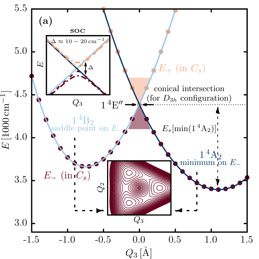
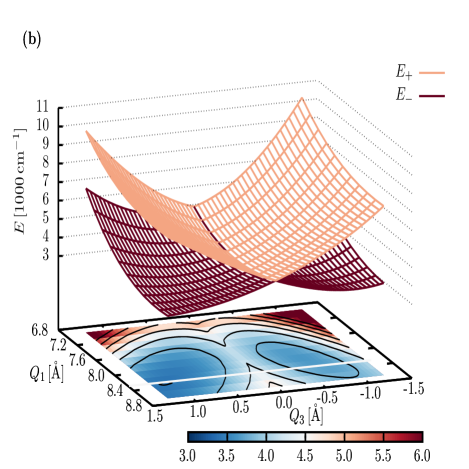
Figure 8: (Color online) The quartet states (according to $C_{2v}$ nomenclature) $1{\,}^{4}\mathrm{B}_{2}$ and $1{\,}^{4}\mathrm{A}_{2}$ forming the Jahn-Teller pair $1{\,}^{4}\mathrm{E}^{\prime\prime}$ in the higher symmetry $D_{3h}$ subspace (equilateral triangle). For each equilateral triangular configuration the two states show a conical intersection (COIN) leading to a COIN seam (one-dimensional curve) in the full 3D configuration space. Lowering the symmetry, e.g. by scanning along the $C_{2v}$ preserving coordinate $Q_{3}$, leads to a splitting of both states (see (a) for $Q_{1}=$8.335\text{\,}\mathrm{\SIUnitSymbolAngstrom}$$ and $Q_{2}=$0.0\text{\,}\mathrm{\SIUnitSymbolAngstrom}$$ fixed). Due to the Jahn-Teller character these states cannot be viewed separately. The interactions lead to the formation of a lower PES sheet $E_{-}$ showing tricorn topology (three equivalent wells alternating regularly with three saddle points, separated by the localization energy $E_{\text{loc}}=225\,\mathrm{cm}^{-1}$) and a parabolic shaped upper surface $E_{+}$. The $1{\,}\tensor{*}[^{4}]{\mathrm{A}}{{}_{2}}$ state represents a global minimum on $E_{-}$ while the $1{\,}\tensor{*}[^{4}]{\mathrm{B}}{{}_{2}}$ state is a saddle point on this surface. This behaviour is illustrated by the lower inset in (a) for $Q_{1}=$8.335\text{\,}\mathrm{\SIUnitSymbolAngstrom}$$. Including spin-orbit coupling (SOC) leads to the annihilation of the COIN and to an energy splitting $\Delta$ as shown by the inset on the top left in (a). The topology of the PESs in the two-dimensional subspace of $Q_{1}$ and $Q_{3}$ is shown in (b). The degenerate line at $Q_{3}=$0.0\text{\,}\mathrm{\SIUnitSymbolAngstrom}$$, where we have $D_{3h}$ symmetry, corresponds to the one-dimensional COIN seam. The white line at the bottom represents the one-dimensional cut shown in (a).

As indicated in Tab. 2 the first excited quartet state $1{\,}\tensor{*}[^{4}]{\mathrm{A}}{{}_{2}}$ forms, together with the $1{\,}\tensor{*}[^{4}]{\mathrm{B}}{{}_{2}}$ state, for equilateral triangular geometries the JT pair $1{\,}\tensor{*}[^{4}]{\mathrm{E}}{{}^{\prime\prime}}$. The two states are degenerate for every high-symmetry ($D_{3h}$) nuclear configuration, thus forming a one-dimensional COIN seam in the full 3D configuration space as already outlined in Sec. II.3. When lowering the symmetry (scanning along $Q_{2}$ and/or $Q_{3}$) both states branch off forming a lower PES sheet $E_{-}$ revealing a tricorn topology with three equivalent minima (of $1{\,}\tensor{*}[^{4}]{\mathrm{A}}{{}_{2}}$ character) alternating regularly with three saddle points (of $1{\,}\tensor{*}[^{4}]{\mathrm{B}}{{}_{2}}$ character) as illustrated by the lower inset in Fig. 8 (a). The upper surface $E_{+}$ is a paraboloid of revolution about $Q_{2}=Q_{3}=0$ Cocchini et al. (1988). Spin-orbit coupling (SOC) removes the COIN with an energy splitting of $\Delta\approx 10-20\,\mathrm{cm}^{-1}$ (i.e. weak SOC) between the corresponding Kramers pairs of $E_{+}$ and $E_{-}$. For details of the underlying (relativistic) JT theory see, e.g., Refs. Bersuker (2001); Rocha and Varandas (2016); Thapaliya et al. (2015); Domcke et al. (2006); Barckholtz and Miller (1998); Poluyanov and Domcke (2008) and Refs. Matsika and Yarkony (2001a, b, 2002), respectively, for the effect of SOC on COINs in general. Here it is important to note that due to the JT interaction the $1{\,}\tensor{*}[^{4}]{\mathrm{A}}{{}_{2}}$ and $1{\,}\tensor{*}[^{4}]{\mathrm{B}}{{}_{2}}$ states cannot be viewed separately. Figure 8 (b) illustrates the one-dimensional COIN seam occurring for $Q_{2}=Q_{3}=0$ and shows a contour plot of the trough of the $E_{-}$–PES in the $D_{3h}$-$C_{2v}$ subspace of $Q_{1}$ and $Q_{3}$. The energetically lowest COIN occurs at $R_{1}=R_{2}=R_{3}=$2.250\text{\,}\mathrm{\SIUnitSymbolAngstrom}$$ with an energy $E_{\text{min}(\text{COIN})}=4146\,\mathrm{cm}^{-1}$ (note that a detailed overview on all JT pairs is given in Tab. LABEL:S-tab:PJTStates in the supplementary material Sup ). It is convenient Cocchini et al. (1988) to define a stabilization energy $E_{s}$ of the minima on $E_{-}$ from the COINs as well as a localization energy $E_{\text{loc}}$ defining the barrier height in the tricorn potential. In the lower inset of Fig. 8 (a) this denotes the energy barrier for transitions between the three equivalent minima on $E_{-}$ separated by three saddle points. The stabilization energy for the cut through the $1{\,}\tensor{*}[^{4}]{\mathrm{A}}{{}_{2}}$ minimum is $E_{s}[\mathrm{min}(1{\,}\tensor{*}[^{4}]{\mathrm{A}}{{}_{2}})]=991\,\mathrm{cm}^{-1}$ as indicated in Fig. 8 (a) and clarified in Fig. LABEL:S-fig:VisualizationEs of the supplementary material Sup . The localization energy is $E_{\text{loc}}=225\,\mathrm{cm}^{-1}$.

III.4 Interactions in the Vicinity of the $1{\,}\tensor{*}[^{4}]{\mathrm{E}}{{}^{\prime\prime}}$ Global Minimum

Despite the small transition dipole strengths between the quartet ground state and the first excited quartet state, discussed above (cf. Fig. 7 (b)), we claim that the $1{\,}\tensor{*}[^{4}]{\mathrm{A}}{{}_{2}}$ state is a promising candidate for PA experiments. First, its minimum is rather well isolated from intersections with doublet and quartet states (both in $C_{2v}$ and $C_{s}$ configuration space) due to the low density of states. Only the $2{\,}\tensor{*}[^{2}]{\mathrm{B}}{{}_{1}}$ and $3{\,}\tensor{*}[^{2}]{\mathrm{A}}{{}_{1}}$ states show intersections, in close proximity to the $1{\,}\tensor{*}[^{4}]{\mathrm{A}}{{}_{2}}$ minimum, besides the symmetry-required one with the $1{\,}\tensor{*}[^{4}]{\mathrm{B}}{{}_{2}}$ state. The energetically closest intersection emerges at $C_{2v}$ geometry with the $3{\,}\tensor{*}[^{2}]{\mathrm{A}}{{}_{1}}$ state for $R_{2}=R_{3}\approx$2.65\text{\,}\mathrm{\SIUnitSymbolAngstrom}$$ and $R_{1}\approx$1.7\text{\,}\mathrm{\SIUnitSymbolAngstrom}$$. For $C_{s}$ geometries intersections with the $2{\,}\tensor{*}[^{2}]{\mathrm{B}}{{}_{1}}$ state move slightly closer to the minimum of the first excited quartet state while the $3{\,}\tensor{*}[^{2}]{\mathrm{A}}{{}_{1}}$ intersections approximately remain at the same location. However, all intersections are $\gtrsim 60\,\mathrm{cm}^{-1}$ away from the $1{\,}\tensor{*}[^{4}]{\mathrm{A}}{{}_{2}}$ global minimum. The situation is illustrated in Fig. LABEL:S-fig:IntersecProximity1A2 of the supplementary material Sup . As indicated previously, the $1{\,}\tensor{*}[^{4}]{\mathrm{A}}{{}_{2}}$ minimum is stabilized from COINs by $E_{s}[\mathrm{min}(1{\,}\tensor{*}[^{4}]{\mathrm{A}}{{}_{2}})]=991\,\mathrm{cm}^{-1}$.

In the vicinity of the $1{\,}\tensor{*}[^{4}]{\mathrm{A}}{{}_{2}}$ equilibrium geometry SOC effects are rather small vanishing with $1/r$ for large $r$ (with $r\propto\sqrt{Q_{2}^{2}+Q_{3}^{2}}$ measuring the distortion from $D_{3h}$ symmetry to acute $C_{2v}$ triangular geometries) as follows from relativistic JT theory Hauser et al. (2010a); Barckholtz and Miller (1998). Strongest SOCs of the $1{\,}\tensor{*}[^{4}]{\mathrm{A}}{{}_{2}}$ state close to its equilibrium geometry are to the quartet ground state $1{\,}\tensor{*}[^{4}]{\mathrm{B}}{{}_{1}}$ as well as to the excited state $1{\,}\tensor{*}[^{4}]{\mathrm{A}}{{}_{1}}$ with typical magnitudes between $30$ to $50\,\mathrm{cm}^{-1}$. The $1{\,}\tensor{*}[^{4}]{\mathrm{A}}{{}_{1}}$ state shows a local minimum at $E_{\text{min}}(1{\,}\tensor{*}[^{4}]{\mathrm{A}}{{}_{1}})=6766\,\mathrm{cm}^{-1}$ (cf. Tab. 2) and is thus well separated from the $1{\,}\tensor{*}[^{4}]{\mathrm{A}}{{}_{2}}$ state. Spin-orbit couplings to doublet states are slightly weaker with interactions between $1{\,}\tensor{*}[^{4}]{\mathrm{A}}{{}_{2}}$ and the $2{\,}\tensor{*}[^{2}]{\mathrm{A}}{{}_{1}}$, $3{\,}\tensor{*}[^{2}]{\mathrm{A}}{{}_{1}}$, $4{\,}\tensor{*}[^{2}]{\mathrm{A}}{{}_{1}}$, $5{\,}\tensor{*}[^{2}]{\mathrm{A}}{{}_{1}}$, $3{\,}\tensor{*}[^{2}]{\mathrm{B}}{{}_{1}}$ and $4{\,}\tensor{*}[^{2}]{\mathrm{B}}{{}_{1}}$ states with orders of $10$ to $30\,\mathrm{cm}^{-1}$. Those equilibrium states are found either well below the minimum of the $1{\,}\tensor{*}[^{4}]{\mathrm{A}}{{}_{2}}$ state at $229\,\mathrm{cm}^{-1}$ or $1898\,\mathrm{cm}^{-1}$, respectively, or well above, starting from $5431\,\mathrm{cm}^{-1}$ (the corresponding values are taken from Tab. LABEL:S-tab:Rb3statesTriangularSupp of the supplementary material Sup ).

IV Summary and Outlook

This work provides a possible roadmap to the experimental realization of PA processes of single ultracold rubidium trimers. We give a wide-ranging overview of available states using the MRCI method, together with a large-core ECP with CPP and a modified even-tempered valence basis-set. By special cuts through the PESs of both low– and high-spin species, we revealed their topology and gave an idea of the mutual position and the expected density of electronic states. We discussed the prominent feature of the (pseudo) Jahn-Teller (JT) effect naturally occuring for triangular geometries and outlined Renner-Teller (combined with pseudo Jahn-Teller) interactions for linear geometries. We also provided a survey of SOC effects giving selection rules and showing that they are weak, particularly for the low-lying states involved in possible PA schemes.

We studied the equilibrium states as well as the locations of selected inner turning points (ITPs) on the quartet ground state PES in the configuration space. Since states lying close to ITPs are promising candidates for good Franck-Condon factors this analysis helped us to identify suitable states for PA processes. We focused on the $1{\,}\tensor{*}[^{4}]{\mathrm{E}}{{}^{\prime\prime}}$ state (consisting of the lowest lying excited states $1{\,}\tensor{*}[^{4}]{\mathrm{A}}{{}_{2}}$ and $1{\,}\tensor{*}[^{4}]{\mathrm{B}}{{}_{2}}$) for which we investigated the characteristic JT topology of the corresponding PES and discussed the consequences of the underlying JT effect. Finally, we investigated the main coupling effects for the first excited quartet state ($1{\,}\tensor{*}[^{4}]{\mathrm{A}}{{}_{2}}$), including electronic dipole transition strengths at ITP geometries, intersections to nearby doublet and quartet states as well as spin-orbit couplings. This confirms the $1{\,}\tensor{*}[^{4}]{\mathrm{A}}{{}_{2}}$ state as a promising candidate for PA experiments.

In a next step we will analyze and fix the breakdown of the Born-Oppenheimer approximation, connected to the various Jahn-Teller coupling effects, by means of different diabatization techniques including diabatic PES interpolation approaches.

Data corresponding to the figures are available in the supplementary material Sup .