Abstract

Generative models are typically trained on grid-like data such as images. As a result, the size of these models usually scales directly with the underlying grid resolution. In this paper, we abandon discretized grids and instead parameterize individual data points by continuous functions. We then build generative models by learning distributions over such functions. By treating data points as functions, we can abstract away from the specific type of data we train on and construct models that are agnostic to discretization. To train our model, we use an adversarial approach with a discriminator that acts on continuous signals. Through experiments on a wide variety of data modalities including images, 3D shapes and climate data, we demonstrate that our model can learn rich distributions of functions independently of data type and resolution.

1 INTRODUCTION

In generative modeling, data is often represented by discrete arrays. Images are represented by two dimensional grids of RGB values, 3D scenes are represented by three dimensional voxel grids and audio as vectors of discretely sampled waveforms. However, the true underlying signal is often continuous. We can therefore also consider representing such signals by continuous functions taking as input grid coordinates and returning features. In the case of images for example, we can define a function $f:\mathbb{R}^{2}\to\mathbb{R}^{3}$ mapping pixel locations to RGB values using a neural network. Such representations, typically referred to as implicit neural representations, coordinate-based neural representations or neural function representations, have the remarkable property that they are independent of signal resolution (Park et al., 2019; Mescheder et al., 2018; Chen and Zhang, 2019; Sitzmann et al., 2020).

In this paper, we build generative models that inherit the attractive properties of implicit representations. By framing generative modeling as learning distributions of functions, we are able to build models that act entirely on continuous spaces, independently of resolution. We achieve this by parameterizing a distribution over neural networks with a hypernetwork (Ha et al., 2017) and training this distribution with an adversarial approach (Goodfellow et al., 2014), using a discriminator that acts directly on sets of coordinates (e.g. pixel locations) and features (e.g. RGB values). Crucially, this allows us to train the model irrespective of any underlying discretization or grid and avoid the curse of discretization (Mescheder, 2020).

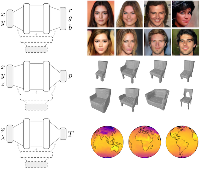
Figure 1: By representing data as continuous functions, we can use the same model to learn distributions of images, 3D shapes and climate data, irrespective of any underlying grid or discretization.

Indeed, standard convolutional generative models act on discretized grids, such as images or voxels, and as a result scale quadratically or cubically with resolution, which quickly becomes intractable at high resolutions, particularly in 3D (Park et al., 2019). In contrast, our model learns distributions on continuous spaces and is agnostic to discretization. This allows us to not only build models that act independently of resolution, but also to learn distributions of functions on manifolds where discretization can be difficult.

To validate our approach, we train generative models on various image, 3D shape and climate datasets. Remarkably, we show that, using our framework, we can learn rich function distributions on these varied datasets using the same model. Further, by taking advantage of recent advances in representing high frequency functions with neural networks (Mildenhall et al., 2020; Tancik et al., 2020; Sitzmann et al., 2020), we also show that, unlike current approaches for generative modeling on continuous spaces (Garnelo et al., 2018a; Mescheder et al., 2019; Kleineberg et al., 2020), we are able to generate sharp and realistic samples.

2 REPRESENTING DATA AS FUNCTIONS

In this section we review implicit neural representations, using images as a guiding example for clarity.

Representing a single image with a function. Let $I$ be an image such that $I[x,y]$ corresponds to the RGB value at pixel location $(x,y)$. We are interested in representing this image by a function $f:\mathbb{R}^{2}\to\mathbb{R}^{3}$ where $f(x,y)=(r,g,b)$ returns the RGB values at pixel location $(x,y)$. To achieve this, we parameterize a function $f_{\theta}$ by an MLP with weights $\theta$, often referred to as an implicit neural representation. We can then learn this representation by minimizing

$$\min_{\theta}\sum_{x,y}\|f_{\theta}(x,y)-I[x,y]\|_{2}^{2},$$

where the sum is over all pixel locations. Remarkably, the representation $f_{\theta}$ is independent of the number of pixels. The representation $f_{\theta}$ therefore, unlike most image representations, does not depend on the resolution of the image (Mescheder et al., 2019; Park et al., 2019; Sitzmann et al., 2020).

Representing general data with functions. The above example with images can readily be extended to more general data. Let $\mathbf{x}\in\mathcal{X}$ denote coordinates and $\mathbf{y}\in\mathcal{Y}$ features and assume we are given a data point as a set of coordinate and feature pairs $\{(\mathbf{x}_{i},\mathbf{y}_{i})\}_{i=1}^{n}$. For an image for example, $\mathbf{x}=(x,y)$ corresponds to pixel locations, $\mathbf{y}=(r,g,b)$ corresponds to RGB values and $\{(\mathbf{x}_{i},\mathbf{y}_{i})\}_{i=1}^{n}$ to the set of all pixel locations and RGB values. Given a set of coordinates and their corresponding features, we can learn a function $f_{\theta}:\mathcal{X}\to\mathcal{Y}$ representing this data point by minimizing

$$\min_{\theta}\sum_{i=1}^{n}\|f_{\theta}(\mathbf{x}_{i})-\mathbf{y}_{i}\|_{2}^{2}.$$ (1)

A core property of these representations is that they scale with signal complexity and not with signal resolution (Sitzmann et al., 2020). Indeed, the memory required to store data scales quadratically with resolution for images and cubically for voxel grids. In contrast, for function representations, the memory requirements scale directly with signal complexity: to represent a more complex signal, we would need to increase the capacity of the function $f_{\theta}$, for example by increasing the number of layers of a neural network.

Figure 2: Modeling an image with a function with (right) and without (left) Fourier features.

Representing high frequency functions. Recently, it has been shown that learning function representations by minimizing equation (1) is biased towards learning low frequency functions (Mildenhall et al., 2020; Sitzmann et al., 2020; Tancik et al., 2020). While several approaches have been proposed to alleviate this problem, we use the random Fourier feature (RFF) encoding proposed by Tancik et al. (2020) as it is not biased towards on axis variation (unlike Mildenhall et al. (2020)) and does not require specialized initialization (unlike Sitzmann et al. (2020)). Specifically, given a coordinate $\mathbf{x}\in\mathbb{R}^{d}$, the encoding function $\gamma:\mathbb{R}^{d}\to\mathbb{R}^{2m}$ is defined as

$$\gamma(\mathbf{x})=\begin{pmatrix}\cos(2\pi B\mathbf{x})\\ \sin(2\pi B\mathbf{x})\end{pmatrix},$$

where $B\in\mathbb{R}^{m\times d}$ is a (potentially learnable) random matrix whose entries are typically sampled from $\mathcal{N}(0,\sigma^{2})$. The number of frequencies $m$ and the variance $\sigma^{2}$ of the entries of $B$ are hyperparameters. To learn high frequency functions, we simply encode $\mathbf{x}$ before passing it through the MLP, $f_{\theta}(\gamma(\mathbf{x}))$, and minimize equation (1). As can be seen in Figure 2, learning a function representation of an image with a ReLU MLP fails to capture high frequency detail whereas using an RFF encoding followed by a ReLU MLP allows us to faithfully reproduce the image.

3 LEARNING DISTRIBUTIONS OF FUNCTIONS

In generative modeling, we are typically given a set of data, such as images, and are interested in approximating the distribution of this data. As we represent data points by functions, we would therefore like to learn a distribution over functions. In the case of images, standard generative models typically sample some noise and feed it through a neural network to output $n$ pixels (Goodfellow et al., 2014; Kingma and Welling, 2014; Rezende et al., 2014). In contrast, we sample the weights of a neural network to obtain a function which we can probe at arbitrary coordinates. Such a representation allows us to operate entirely on coordinates and features irrespective of any underlying grid representation that may be available. To train the function distribution we use an adversarial approach and refer to our model as a Generative Adversarial Stochastic Process (GASP).

3.1 Data Representation

While our goal is to learn a distribution over functions, we typically do not have access to the ground truth functions representing the data. Instead, each data point is typically given by some set of coordinates and features $\mathbf{s}=\{(\mathbf{x}_{i},\mathbf{y}_{i})\}_{i=1}^{n}$. For an image for example, we do not have access to a function mapping pixel locations to RGB values but to a collection of $n$ pixels. Such a set of coordinates and features corresponds to input/output pairs of a function, allowing us to learn function distributions without operating directly on the functions. A single data point then corresponds to a set of coordinates and features (e.g. an image is a set of $n$ pixels). We then assume a dataset is given as samples $\mathbf{s}\sim p_{\text{data}}(\mathbf{s})$ from a distribution over sets of coordinate and feature pairs. Working with sets of coordinates and features is very flexible - such a representation is agnostic to whether the data originated from a grid and at which resolution it was sampled.

Crucially, formulating our problem entirely on sets also lets us split individual data points into subsets and train on those. Specifically, given a single data point $\mathbf{s}=\{(\mathbf{x}_{i},\mathbf{y}_{i})\}_{i=1}^{n}$, such as a collection of $n$ pixels, we can randomly subsample $K$ elements, e.g. we can select $K$ pixels among the $n$ pixels in the entire image. Training on such subsets then removes any direct dependence on the resolution of the data. For example, when training on 3D shapes, instead of passing an entire voxel grid to the model, we can train on subsets of the voxel grid, leading to large memory savings (see Section 5.2). This is not possible with standard convolutional models which are directly tied to the resolution of the grid. Further, training on sets of coordinates and features allows us to model more exotic data, such as distributions of functions on manifolds (see Section 5.3). Indeed, as long as we can define a coordinate system on the manifold (such as polar coordinates on a sphere), our method applies.

3.2 Function Generator

Learning distributions of functions with an adversarial approach requires us to define a generator that generates fake functions and a discriminator that distinguishes between real and fake functions. We define the function generator using the commonly applied hypernetwork approach (Ha et al., 2017; Sitzmann et al., 2019, 2020; Anokhin et al., 2021; Skorokhodov et al., 2021). More specifically, we assume the structure (e.g. the number and width of layers) of the MLP $f_{\theta}$ representing a single data point is fixed. Learning a distribution over functions $f_{\theta}$ is then equivalent to learning a distribution over weights $p(\theta)$. The distribution $p(\theta)$ is defined by a latent distribution $p(\mathbf{z})$ and a second function $g_{\phi}:\mathcal{Z}\to\Theta$, itself with parameters $\phi$, mapping latent variables to the weights $\theta$ of $f_{\theta}$ (see Figure 3). We can then sample from $p(\theta)$ by sampling $\mathbf{z}\sim p(\mathbf{z})$ and mapping $\mathbf{z}$ through $g_{\phi}$ to obtain a set of weights $\theta=g_{\phi}(\mathbf{z})$. After sampling a function $f_{\theta}$, we then evaluate it at a set of coordinates $\{\mathbf{x}_{i}\}$ to obtain a set of generated features $\{\mathbf{y}_{i}\}$ which can be used to train the model. Specifically, given a latent vector $\mathbf{z}$ and a coordinate $\mathbf{x}_{i}$, we compute a generated feature as $\mathbf{y}_{i}=f_{g_{\phi}(\mathbf{z})}(\gamma(\mathbf{x}_{i}))$ where $\gamma$ is an RFF encoding allowing us to learn high frequency functions.

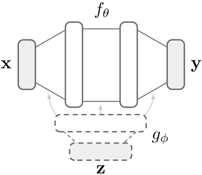
Figure 3: Diagram of a neural function distribution architecture. A latent vector $\mathbf{z}$ is mapped through a hypernetwork $g_{\phi}$ (in dashed lines) to obtain the weights of a function $f_{\theta}$ (in solid lines) mapping coordinates $\mathbf{x}$ to features $\mathbf{y}$.

3.3 Point Cloud Discriminator

In the GAN literature, discriminators are almost always parameterized with convolutional neural networks (CNN). However, the data we consider may not necessarily lie on a grid, in which case it is not possible to use convolutional discriminators. Further, convolutional discriminators scale directly with grid resolution (training a CNN on images at $2\times$ the resolution requires $4\times$ the memory) which partially defeats the purpose of using implicit representations.

As the core idea of our paper is to build generative models that are independent of discretization, we therefore cannot follow the naive approach of using convolutional discriminators. Instead, our discriminator should be able to distinguish between real and fake sets of coordinate and feature pairs. Specifically, we need to define a function $D$ which takes in an unordered set $\mathbf{s}$ and returns the probability that this set represents input/output pairs of a real function. We therefore need $D$ to be permutation invariant with respect to the elements of the set $\mathbf{s}$. The canonical choice for set functions is the PointNet (Qi et al., 2017) or DeepSets (Zaheer et al., 2017) model family. However, we experimented extensively with such functions and found that they were not adequate for learning complex function distributions (see Section 3.5). Indeed, while the input to the discriminator is an unordered set $\mathbf{s}=\{(\mathbf{x}_{i},\mathbf{y}_{i})\}$, there is an underlying notion of distance between points $\mathbf{x}_{i}$ in the coordinate space. We found that it is crucial to take this into account when training models on complex datasets. Indeed, we should not consider the coordinate and feature pairs as sets but rather as point clouds (i.e. sets with an underlying notion of distance).

While several works have tackled the problem of point cloud classification (Qi et al., 2017; Li et al., 2018; Thomas et al., 2019), we leverage the PointConv framework introduced by Wu et al. (2019) for several reasons. Firstly, PointConv layers are translation equivariant (like regular convolutions) and permutation invariant by construction. Secondly, when sampled on a regular grid, PointConv networks closely match the performance of regular CNNs. Indeed, we can loosely think of PointConv as a continuous equivalent of CNNs and, as such, we can build PointConv architectures that are analogous to typical discriminator architectures.

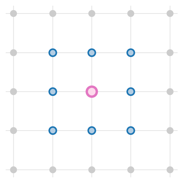
Figure 4: Convolution neighborhood for regular convolutions (left) and PointConv (right).

Specifically, we assume we are given a set of features $\mathbf{f}_{i}\in\mathbb{R}^{c_{\text{in}}}$ at locations $\mathbf{x}_{i}$ (we use $\mathbf{f}_{i}$ to distinguish these hidden features of the network from input features $\mathbf{y}_{i}$). In contrast to regular convolutions, where the convolution kernels are only defined at certain grid locations, the convolution filters in PointConv are parameterized by an MLP, $W:\mathbb{R}^{d}\to\mathbb{R}^{c_{\text{out}}\times c_{\text{in}}}$, mapping coordinates to kernel values. We can therefore evaluate the convolution filters in the entire coordinate space. The PointConv operation at a point $\mathbf{x}$ is then defined as

$$\mathbf{f}_{\text{out}}(\mathbf{x})=\sum_{\mathbf{x}_{i}\in N_{\mathbf{x}}}W(\mathbf{x}_{i}-\mathbf{x})\mathbf{f}_{i},$$

where $N_{\mathbf{x}}$ is a set of neighbors of $\mathbf{x}$ over which to perform the convolution (see Figure 4). Interestingly, this neighborhood is found by a nearest neighbor search with respect to some metric on the coordinate space. We therefore have more flexibility in defining the convolution operation as we can choose the most appropriate notion of distance for the space we want to model (our implementation supports fast computation on the GPU for any $\ell_{p}$ norm).

Generated data                             Real data                     Discriminator

Figure 5: Training procedure for GASP: 1. Sample a function and evaluate it at a set of coordinate locations to generate fake point cloud. 2. Convert real data sample to point cloud. 3. Discriminate between real and fake point clouds.

3.4 Training

We use the traditional (non saturating) GAN loss (Goodfellow et al., 2014) for training and illustrate the entire procedure for a single training step in Figure 5. To stabilize training, we define an equivalent of the $R_{1}$ penalty from Mescheder et al. (2018) for point clouds. For images, $R_{1}$ regularization corresponds to penalizing the gradient norm of the discriminator with respect to the input image. For a set $\mathbf{s}=\{(\mathbf{x}_{i},\mathbf{y}_{i})\}_{i=1}^{n}$, we define the penalty as

$$R_{1}(\mathbf{s})=\frac{1}{2}\|\nabla_{\mathbf{y}_{1},\dots,\mathbf{y}_{n}}D(\mathbf{s})\|^{2}=\frac{1}{2}\sum_{\mathbf{y}_{i}}\|\nabla_{\mathbf{y}_{i}}D(\mathbf{s})\|^{2},$$

that is we penalize the gradient norm of the discriminator with respect to the features. Crucially, our entire modeling procedure is then independent of discretization. Indeed, the generator, discriminator and loss all act directly on continuous point clouds.

3.5 How Not to Learn Distributions of Functions

In developing our model, we found that several approaches which intuitively seem appropriate for learning distributions of functions do not work in the context of generative modeling. We briefly describe these here and provide details and proofs in the appendix.

Set discriminators. As described in Section 3.3, the canonical choice for set functions is the PointNet/DeepSet model family (Qi et al., 2017; Zaheer et al., 2017). Indeed, Kleineberg et al. (2020) use a similar approach to ours to learn signed distance functions for 3D shapes using such a set discriminator. However, we found both theoretically and experimentally that PointNet/DeepSet functions were not suitable as discriminators for complex function distributions (such as natural images). Indeed, these models do not directly take advantage of the metric on the space of coordinates, which we conjecture is crucial for learning rich function distributions. In addition, we show in the appendix that the Lipschitz constant of set functions can be very large, leading to unstable GAN training (Arjovsky et al., 2017; Roth et al., 2017; Mescheder et al., 2018). We provide further theoretical and experimental insights on set discriminators in the appendix.

Auto-decoders. A common method for embedding functions into a latent space is the auto-decoder framework used in DeepSDF (Park et al., 2019). This framework and variants of it have been extensively used in 3D computer vision (Park et al., 2019; Sitzmann et al., 2019). While auto-decoders excel at a variety of tasks, we show in the appendix that the objective used to train these models is not appropriate for generative modeling. We provide further analysis and experimental results on auto-decoders in the appendix.

While none of the above models were able to learn function distributions on complex datasets such as CelebAHQ, all of them worked well on MNIST. We therefore believe that MNIST is not a meaningful benchmark for generative modeling of functions and encourage future research in this area to include experiments on more complex datasets.

4 RELATED WORK

Implicit representations. Implicit representations were initially introduced in the context of evolutionary algorithms as compositional pattern producing networks (Stanley, 2007). In pioneering work, Ha (2016) built generative models of such networks for MNIST. Implicit representations for 3D geometry were initially (and concurrently) proposed by (Park et al., 2019; Mescheder et al., 2019; Chen and Zhang, 2019). A large body of work has since taken advantage of these representations for inverse rendering (Sitzmann et al., 2019; Mildenhall et al., 2020; Niemeyer et al., 2020; Yu et al., 2021), modeling dynamic scenes (Niemeyer et al., 2019; Pumarola et al., 2021), modeling 3D scenes (Atzmon and Lipman, 2020; Jiang et al., 2020; Gropp et al., 2020) and superresolution (Chen et al., 2021).

Continuous models of image distributions. In addition to the work of Ha (2016), neural processes (Garnelo et al., 2018a, b) are another family of models that can learn (conditional) distributions of images as functions. However, the focus of these is on uncertainty quantification and meta-learning rather than generative modeling. Further, these models do not scale to large datasets, although adding attention (Kim et al., 2019) and translation equivariance (Gordon et al., 2019) helps alleviate this. Gradient Origin Networks (Bond-Taylor and Willcocks, 2021) model distributions of implicit representations using an encoder free model, instead using gradients of the latents as an encoder. In concurrent work, Skorokhodov et al. (2021); Anokhin et al. (2021) use an adversarial approach to learn distributions of high frequency implicit representations for images. Crucially, these both use standard image convolutional discriminators and as such do not inherit several advantages of implicit representations: they are restricted to data lying on a grid and suffer from the curse of discretization. In contrast, GASP is entirely continuous and independent of resolution and, as a result, we are able to train on a variety of data modalities.

Continuous models of 3D shape distributions. Mescheder et al. (2019) use a VAE to learn distributions of occupancy networks for 3D shapes, while Chen and Zhang (2019) train a GAN on embeddings of a CNN autoencoder with an implicit function decoder. Park et al. (2019); Atzmon and Lipman (2021) parameterize families of 3D shapes using the auto-decoder framework, which, as shown in Section 3.5, cannot be used for sampling. Kleineberg et al. (2020) use a set discriminator to learn distributions of signed distance functions for 3D shape modeling. However, we show both theoretically (see appendix) and empirically (see Section 5) that using such a set discriminator severely limits the ability of the model to learn complex function distributions. Cai et al. (2020) represent functions implicitly by gradient fields and use Langevin sampling to generate point clouds. Spurek et al. (2020) learn a function mapping a latent vector to a point cloud coordinate, which is used for point cloud generation. In addition, several recent works have tackled the problem of learning distributions of NeRF scenes (Mildenhall et al., 2020), which are special cases of implicit representations. This includes GRAF (Schwarz et al., 2020) which concatenates a latent vector to an implicit representation and trains the model adversarially using a patch-based convolutional discriminator, GIRAFFE (Niemeyer and Geiger, 2021) which adds compositionality to the generator and pi-GAN (Chan et al., 2021) which models the generator using modulations to the hidden layer activations. Finally, while some of these works show basic results on small scale image datasets, GASP is, to the best of our knowledge, the first work to show how function distributions can be used to model a very general class of data, including images, 3D shapes and data lying on manifolds.

5 EXPERIMENTS

We evaluate our model on CelebAHQ (Karras et al., 2018) at $64\times 64$ and $128\times 128$ resolution, on 3D shapes from the ShapeNet (Chang et al., 2015) chairs category and on climate data from the ERA5 dataset (Hersbach et al., 2019). For all datasets we use the exact same model except for the input and output dimensions of the function representation and the parameters of the Fourier features. Specifically, we use an MLP with 3 hidden layers of size 128 for the function representation and an MLP with 2 hidden layers of size 256 and 512 for the hypernetwork. Remarkably, we find that such a simple architecture is sufficient for learning rich distributions of images, 3D shapes and climate data.

The point cloud discriminator is loosely based on the DCGAN architecture (Radford et al., 2015). Specifically, for coordinates of dimension $d$, we use $3^{d}$ neighbors for each PointConv layer and downsample points by a factor of $2^{d}$ at every pooling layer while doubling the number of channels. We implemented our model in PyTorch (Paszke et al., 2019) and performed all training on a single 2080Ti GPU with 11GB of RAM. The code can be found at https://github.com/EmilienDupont/neural-function-distributions.

5.1 Images

We first evaluate our model on the task of image generation. To generate images, we sample a function from the learned model and evaluate it on a grid. As can be seen in in Figure 6, GASP produces sharp and realistic images both at $64\times 64$ and $128\times 128$ resolution. While there are artifacts and occasionally poor samples (particularly at $128\times 128$ resolution), the images are generally convincing and show that the model has learned a meaningful distribution of functions representing the data. To the best of our knowledge, this is the first time data of this complexity has been modeled in an entirely continuous fashion.

As the representations we learn are independent of resolution, we can examine the continuity of GASP by generating images at higher resolutions than the data on which it was trained. We show examples of this in Figure 7 by first sampling a function from our model, evaluating it at the resolution on which it was trained and then evaluating it at a $4\times$ higher resolution. As can be seen, our model generates convincing $256\times 256$ images even though it has only seen $64\times 64$ images during training, confirming the continuous nature of GASP (see appendix for more examples).

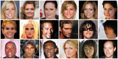
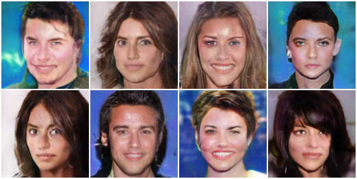
Figure 6: Samples from our model trained on CelebAHQ $64\times 64$ (top) and $128\times 128$ (bottom). Each image corresponds to a function which was sampled from our model and then evaluated on the grid. To produce this figure we sampled 5 batches and chose the best batch by visual inspection.

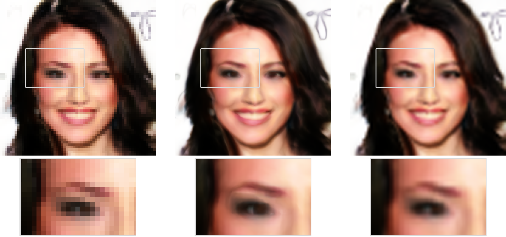
Figure 7: Superresolution. The first column corresponds to the original resolution, the second column to $4\times$ the resolution and the third column to bicubic upsampling.

We compare GASP against three baselines: a model trained using the auto-decoder (AD) framework (similar to DeepSDF (Park et al., 2019)), a model trained with a set discriminator (SD) (similar to Kleineberg et al. (2020)) and a convolutional neural process (ConvNP) (Gordon et al., 2019). To the best of our knowledge, these are the only other model families that can learn generative models in a continuous manner, without relying on a grid representation (which is required for regular CNNs). Results comparing all three models on CelebAHQ $32\times 32$ are shown in Figure 8. As can be seen, the baselines generate blurry and incoherent samples, while our model is able to generate sharp, diverse and plausible samples. Quantitatively, our model (Table 1) outperforms all baselines, although it lags behind state of the art convolutional GANs specialized to images (Lin et al., 2019).

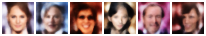
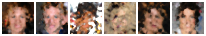
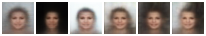
AD SD ConvNP GASP

Figure 8: Baseline comparisons on CelebAHQ $32\times 32$. Note that the ConvNP model was trained on CelebA (not CelebAHQ) and as such has a different crop.

	CelebAHQ64	CelebAHQ128
SD	236.82	-
AD	117.80	-
GASP	7.42	19.16
Conv	4.00	5.74

Table 1: FID scores (lower is better) for various models on CelebAHQ datasets, including a standard convolutional image GAN (Lin et al., 2019).

5.2 3D Scenes

To test the versatility and scalability of GASP, we also train it on 3D shapes. To achieve this, we let the function representation $f_{\theta}:\mathbb{R}^{3}\to\mathbb{R}$ map $x,y,z$ coordinates to an occupancy value $p$ (which is 0 if the location is empty and 1 if it is part of an object). To generate data, we follow the setup from Mescheder et al. (2019). Specifically, we use the voxel grids from Choy et al. (2016) representing the chairs category from ShapeNet (Chang et al., 2015). The dataset contains 6778 chairs each of dimension $32^{3}$. As each 3D model is large (a set of $32^{3}=32,768$ points), we uniformly subsample $K=4096$ points from each object during training, which leads to large memory savings (Figure 9) and allows us to train with large batch sizes even on limited hardware. Crucially, this is not possible with convolutional discriminators and is a key property of our model: we can train the model independently of the resolution of the data.

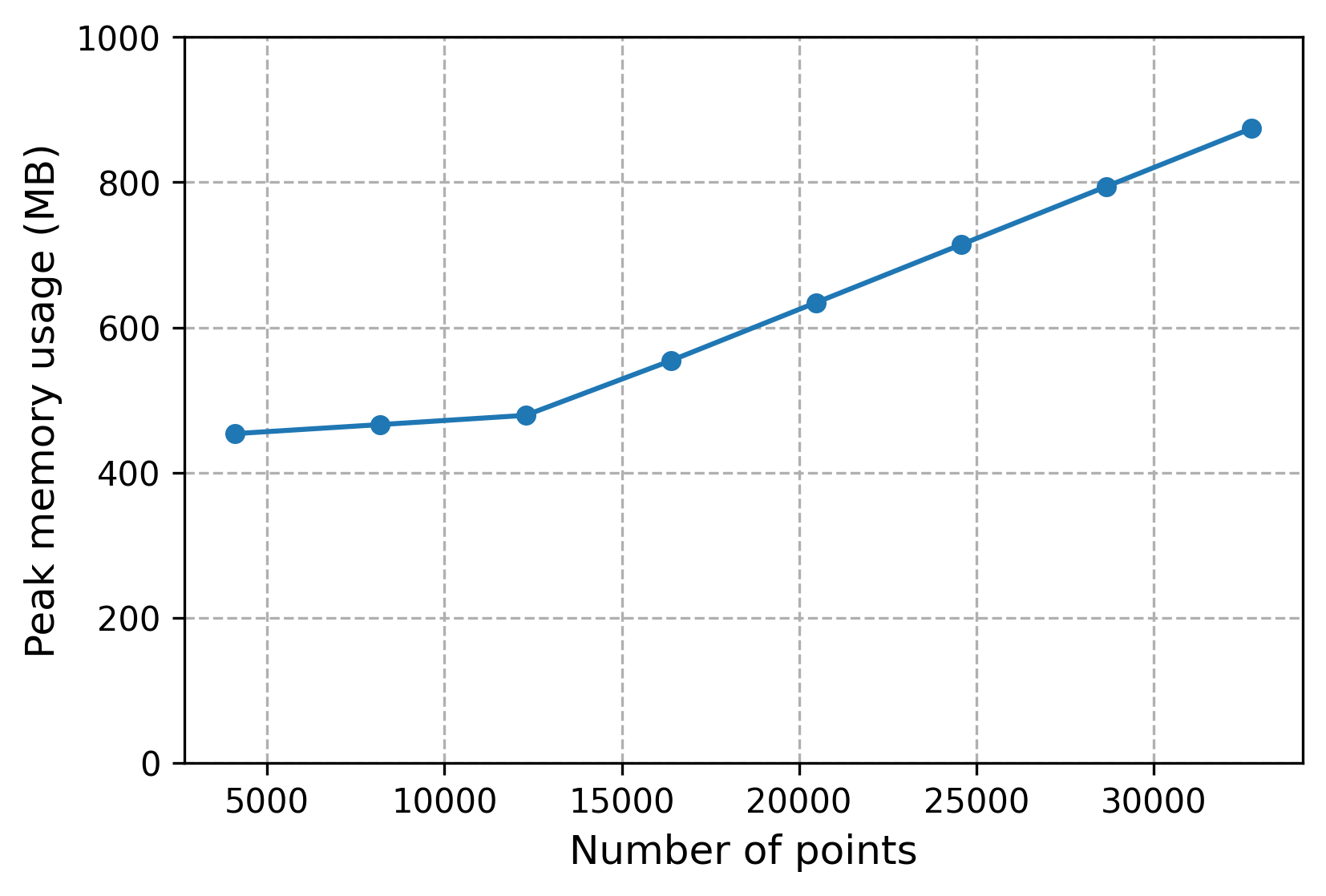
Figure 9: GPU memory consumption as a function of the number of points $K$ in voxel grid.

$16^{3}$           $32^{3}$           $64^{3}$           $128^{3}$

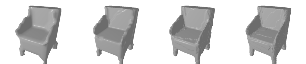
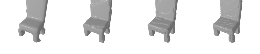
Figure 10: Evaluating the same function at different resolutions. As samples from our model can be probed at arbitrary coordinates, we can increase the resolution to render smoother meshes.

In order to visualize results, we convert the functions sampled from GASP to meshes we can render (see appendix for details). As can be seen in Figure 10, the continuous nature of the data representation allows us to sample our model at high resolutions to produce clean and smooth meshes. In Figure 11, we compare our model to two strong baselines for continuous 3D shape modeling: occupancy networks trained as VAEs (Mescheder et al., 2019) and DeepSDFs trained with a set discriminator approach (Kleineberg et al., 2020). As can be seen, GASP produces coherent and fairly diverse samples, which are comparable to both baselines specialized to 3D shapes.

GASP     SD       ON    

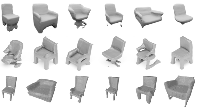
Figure 11: Samples from occupancy networks trained as VAEs (ON), DeepSDF with set discriminators (SD) and GASP trained on ShapeNet chairs. The top row samples were taken from Mescheder et al. (2019) and the middle row samples from Kleineberg et al. (2020).

5.3 Climate Data

As we have formulated our framework entirely in terms of continuous coordinates and features, we can easily extend GASP to learning distributions of functions on manifolds. We test this by training GASP on temperature measurements over the last 40 years from the ERA5 dataset (Hersbach et al., 2019), where each datapoint is a $46\times 90$ grid of temperatures $T$ measured at evenly spaced latitudes $\lambda$ and longitudes $\varphi$ on the globe (see appendix for details). The dataset is composed of 8510 such grids measured at different points in time. We then model each datapoint by a function $f:S^{2}\to\mathbb{R}$ mapping points on the sphere to temperatures. We treat the temperature grids as i.i.d. samples and therefore do not model any temporal correlation, although we could in principle do this by adding time $t$ as an input to our function.

To ensure the coordinates lie on a manifold, we simply convert the latitude-longitude pairs to spherical coordinates before passing them to the function representation, i.e. we set $\mathbf{x}=(\cos\lambda\cos\varphi,\cos\lambda\sin\varphi,\sin\lambda)$. We note that, in contrast to standard discretized approaches which require complicated models to define convolutions on the sphere (Cohen et al., 2018; Esteves et al., 2018), we only need a coordinate system on the manifold to learn distributions.

While models exist for learning conditional distributions of functions on manifolds using Gaussian processes (Borovitskiy et al., 2021; Jensen et al., 2020), we are not aware of any work learning unconditional distributions of such functions for sampling. As a baseline we therefore compare against a model trained directly on the grid of latitudes and longitudes (thereby ignoring that the data comes from a manifold). Samples from our model as well as comparisons with the baseline and an example of interpolation in function space are shown in Figure 12. As can be seen, GASP generates plausible samples, smooth interpolations and, unlike the baseline, is continuous across the sphere.

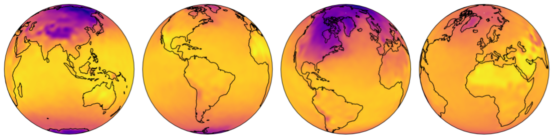
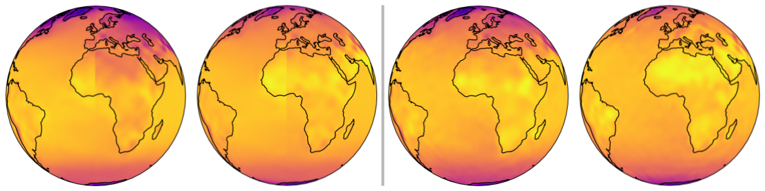
Samples Baseline Interpolation

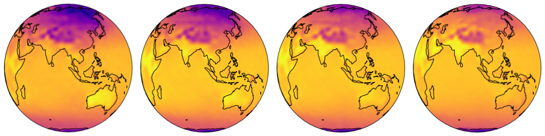
Figure 12: Results on climate data. The top row shows samples from our model. The middle row shows comparisons between GASP (on the right) and a baseline (on the left) trained on a grid. As can be seen, the baseline generates discontinuous samples at the grid boundary unlike GASP which produces smooth samples. The bottom row shows a latent interpolation corresponding roughly to interpolating between summer and winter in the northern hemisphere.

6 SCOPE, LIMITATIONS AND FUTURE WORK

Limitations. While learning distributions of functions gives rise to very flexible generative models applicable to a wide variety of data modalities, GASP does not outperform state of the art specialized image and 3D shape models. We strived for simplicity when designing our model but hypothesize that standard GAN tricks (Karras et al., 2018, 2019; Arjovsky et al., 2017; Brock et al., 2019) could help narrow this gap in performance. In addition, we found that training could be unstable, particularly when subsampling points. On CelebAHQ for example, decreasing the number of points per example also decreases the quality of the generated images (see appendix for samples and failure examples), while the 3D model typically collapses to generating simple shapes (e.g. four legged chairs) even if the data contains complex shapes (e.g. office chairs). We conjecture that this is due to the nearest neighbor search in the discriminator: when subsampling points, a nearest neighbor may lie very far from a query point, potentially leading to unstable training. More refined sampling methods and neighborhood searches should help improve stability. Finally, determining the neighborhood for the point cloud convolution can be expensive when a large number of points is used, although this could be mitigated with faster neighbor search (Johnson et al., 2019).

Future work. As our model formulation is very flexible, it would be interesting to apply GASP to geospatial (Jean et al., 2016), geological (Dupont et al., 2018), meteorological (Sønderby et al., 2020) or molecular (Wu et al., 2018) data which typically do not lie on a regular grid. In computer vision, we hope our approach will help scale generative models to larger datasets. While our model in its current form could not scale to truly large datasets (such as room scale 3D scenes), framing generative models entirely in terms of coordinates and features could be a first step towards this. Indeed, while grid-based generative models currently outperform continuous models, we believe that, at least for certain data modalities, continuous models will eventually surpass their discretized counterparts.

7 CONCLUSION

In this paper, we introduced GASP, a method for learning generative models that act entirely on continuous spaces and as such are independent of signal discretization. We achieved this by learning distributions over functions representing the data instead of learning distributions over the data directly. Through experiments on images, 3D shapes and climate data, we showed that our model learns rich function distributions in an entirely continuous manner. We hope such a continuous approach will eventually enable generative modeling on data that is not currently tractable, either because discretization is expensive (such as in 3D) or difficult (such as on non-euclidean data).

Acknowledgements

We thank William Zhang, Yuyang Shi, Jin Xu, Valentin De Bortoli, Jean-Francois Ton and Kaspar Märtens for providing feedback on an early version of the paper. We also thank Charline Le Lan, Jean-Francois Ton and Bobby He for helpful discussions. We thank Yann Dubois for providing the ConvNP samples as well as helpful discussions around neural processes. We thank Shahine Bouabid for help with the ERA5 climate data. Finally, we thank the anonymous reviewers and the ML Collective for providing constructive feedback that helped us improve the paper. Emilien gratefully acknowledges his PhD funding from Google DeepMind.

 

Supplementary Material:
Generative Models as Distributions of Functions

 

Appendix A EXPERIMENTAL DETAILS

In this section we provide experimental details necessary to reproduce all results in the paper. All the models were implemented in PyTorch Paszke et al. (2019) and trained on a single 2080Ti GPU with 11GB of RAM. The code to reproduce all experiments can be found at https://github.com/EmilienDupont/neural-function-distributions.

A.1 Single Image Experiment

To produce Figure 2, we trained a ReLU MLP with 2 hidden layers each with 256 units, using tanh as the final non-linearity. We trained for 1000 iterations with Adam using a learning rate of 1e-3. For the RFF encoding we set $m=256$ and $\sigma=10$.

A.2 GASP Experiments

For all experiments (images, 3D shapes and climate data), we parameterized $f_{\theta}$ by an MLP with 3 hidden layers, each with 128 units. We used a latent dimension of 64 and an MLP with 2 hidden layers of dimension 256 and 512 for the hypernetwork $g_{\phi}$. We normalized all coordinates to lie in $[-1,1]^{d}$ and all features to lie in $[-1,1]^{k}$. We used LeakyReLU non-linearities both in the generator and discriminator. The final output of the function representation was followed by a tanh non-linearity.

For the point cloud discriminator, we used $3^{d}$ neighbors in each convolution layer and followed every convolution by an average pooling layer reducing the number of points by $2^{d}$. We applied a sigmoid as the final non-linearity. We used an MLP with 4 hidden layers each of size 16 to parameterize all weight MLPs. Unless stated otherwise, we use Adam with a learning rate of 1e-4 for the hypernetwork weights and 4e-4 for the discriminator weights with $\beta_{1}=0.5$ and $\beta_{2}=0.999$ as is standard for GAN training. For each dataset, we trained for a large number of epochs and chose the best model by visual inspection.

MNIST

• Dimensions: $d=2$, $k=1$

• Fourier features: $m=128$, $\sigma=1$

• Discriminator channels: $64,128,256$

• Batch size: 128

• Epochs: 150

CelebAHQ 64x64

• Dimensions: $d=2$, $k=3$

• Fourier features: $m=128$, $\sigma=2$

• Discriminator channels: $64,128,256,512$

• Batch size: 64

• Epochs: 300

CelebAHQ 128x128

• Dimensions: $d=2$, $k=3$

• Fourier features: $m=128$, $\sigma=3$

• Discriminator channels: $64,128,256,512,1024$

• Batch size: 22

• Epochs: 70

ShapeNet voxels

• Dimensions: $d=3$, $k=1$

• Fourier features: None

• Discriminator channels: $32,64,128,256$

• Batch size: 24

• Learning rates: Generator 2e-5, Discriminator 8e-5

• Epochs: 200

ERA5 climate data

• Dimensions: $d=2$, $k=1$

• Fourier features: $m=128$, $\sigma=2$

• Discriminator channels: $64,128,256,512$

• Batch size: 64

• Epochs: 300

A.3 Things We Tried That Didn’t Work

• We initially let the function representation $f_{\theta}$ have 2 hidden layers of size 256, instead of 3 layers of size 128. However, we found that this did not work well, particularly for more complex datasets. We hypothesize that this is because the number of weights in a single $256\to 256$ linear layer is $4\times$ the number of weights in a single $128\to 128$ layer. As such, the number of weights in four $128\to 128$ layers is the same as a single $256\to 256$, even though such a 4-layer network would be much more expressive. Since the hypernetwork needs to output all the weights of the function representation, the final layer of the hypernetwork will be extremely large if the number of function weights is large. It is therefore important to make the network as expressive as possible with as few weights as possible, i.e. by making the network thinner and deeper.

• As the paper introducing the $R_{1}$ penalty (Mescheder et al., 2018) does not use batchnorm (Ioffe and Szegedy, 2015) in the discriminator, we initially ran experiments without using batchnorm. However, we found that using batchnorm both in the weight MLPs and between PointConv layers was crucial for stable training. We hypothesize that this is because using standard initializations for the weights of PointConv layers would result in PointConv outputs (which correspond to the weights in regular convolutions) that are large. Adding batchnorm fixed this initialization issue and resulted in stable training.

• In the PointConv paper, it was shown that the number of hidden layers in the weight MLPs does not significantly affect classification performance (Wu et al., 2019). We therefore initially experimented with single hidden layer MLPs for the weights. However, we found that it is crucial to use deep networks for the weight MLPs in order to build discriminators that are expressive enough for the datasets we consider.

• We experimented with learning the frequencies of the Fourier features (i.e. learning $B$) but found that this did not significantly boost performance and generally resulted in slower training.

A.4 ERA5 Climate Data

We extracted the data used for the climate experiments from the ERA5 database (Hersbach et al., 2019). Specifically, we used the monthly averaged surface temperature at 2m, with reanalysis by hour of day. Each data point then corresponds to a set of temperature measurements on a 721 x 1440 grid (i.e. 721 latitudes and 1440 longitudes) across the entire globe (corresponding to measurements every 0.25 degrees). For our experiments, we subsample this grid by a factor of 16 to obtain grids of size 46 x 90. For each month, there are a total of 24 grids, corresponding to each hour of the day. The dataset is then composed of temperature measurements for all months between January 1979 and December 2020, for a total of 12096 datapoints. We randomly split this dataset into a train set containing 8510 grids, a validation set containing 1166 grids and a test set containing 2420 grids. Finally, we normalize the data to lie in $[0,1]$ with the lowest temperature recorded since 1979 corresponding to 0 and the highest temperature to 1.

A.5 Quantitative Experiments

We computed FID scores using the pytorch-fid library (Seitzer, 2020). We generated 30k samples for both CelebAHQ $64\times 64$ and $128\times 128$ and used default settings for all hyperparameters. We note that the FID scores for the convolutional baselines in the main paper were computed on CelebA (not the HQ version) and are therefore not directly comparable with our model. However, convolutional GANs would also outperform our model on CelebAHQ.

A.6 Rendering 3D Shapes

In order to visualize results for the 3D experiments, we convert the functions sampled from GASP to meshes we can render. To achieve this, we first sample a function from our model and evaluate it on a high resolution grid (usually $128^{3}$). We then threshold the values of this grid at $0.5$ (we found the model was robust to choices of threshold) so voxels with values above the threshold are occupied while the rest are empty. Finally, we use the marching cubes algorithm (Lorensen and Cline, 1987) to convert the grid to a 3D mesh which we render with PyTorch3D (Ravi et al., 2020).

A.7 Baseline Experiments

The baseline models in Section 5.1 were trained on CelebAHQ $32\times 32$, using the same generator as the one used for the CelebAHQ $64\times 64$ experiments. Detailed model descriptions can be found in Section B and hyperparameters are provided below.

Auto-decoders. We used a batch size of 64 and a learning rate of 1e-4 for both the latents and the generator parameters. We sampled the latent initializations from $\mathcal{N}(0,0.01^{2})$. We trained the model for 200 epochs and chose the best samples based on visual inspection.

Set Discriminators. We used a batch size of 64, a learning rate of 1e-4 for the generator and a learning rate of 4e-4 for the discriminator. We used an MLP with dimensions [512, 512, 512] for the set encoder layers and an MLP with dimensions [256, 128, 64, 32, 1] for the final discriminator layers. We used Fourier features with $m=128$, $\sigma=2$ for both the coordinates and the features before passing them to the set discriminator. We trained the model for 200 epochs and chose the best samples based on visual inspection.

Appendix B MODELS THAT ARE NOT SUITABLE FOR LEARNING FUNCTION DISTRIBUTIONS

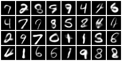
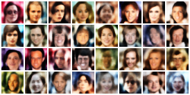
Figure 13: Left: Samples from an auto-decoder model trained on MNIST. Right: Samples from an auto-decoder model trained on CelebAHQ $32\times 32$.

B.1 Auto-decoders

We briefly introduce auto-decoder models following the setup in (Park et al., 2019) and describe why they are not suitable as generative models. As in the GASP case, we assume we are given a dataset of $N$ samples $\{\mathbf{s}^{(i)}\}_{i=1}^{N}$ (where each sample $\mathbf{s}^{(i)}$ is a set). We then associate a latent vector $\mathbf{z}^{(i)}$ with each sample $\mathbf{s}^{(i)}$. We further parameterize a probabilistic model $p_{\theta}(\mathbf{s}^{(i)}|\mathbf{z}^{(i)})$ (similar to the decoder in variational autoencoders) by a neural network with learnable parameters $\theta$ (typically returning the mean of a Gaussian with fixed variance). The optimal parameters are then estimated as

$$\arg\!\max_{\theta,\{\mathbf{z}^{(i)}\}}\sum_{i=1}^{N}\log p_{\theta}(\mathbf{s}^{(i)}|\mathbf{z}^{(i)})+\log p(\mathbf{z}^{(i)}),$$

where $p(\mathbf{z})$ is a (typically Gaussian) prior over the $\mathbf{z}^{(i)}$’s. Crucially the latents vectors $\mathbf{z}^{(i)}$ are themselves learnable and optimized. However, maximizing $\log p(\mathbf{z}^{(i)})\propto-\|\mathbf{z}^{(i)}\|^{2}$ does not encourage the $\mathbf{z}^{(i)}$’s to be distributed according to the prior, but only encourages them to have a small norm. Note that this is because we are optimizing the samples and not the parameters of the Gaussian prior. As such, after training, the $\mathbf{z}^{(i)}$’s are unlikely to be distributed according to the prior. Sampling from the prior to generate new samples from the model will therefore not work.

We hypothesize that this is why the prior is required to have very low variance for the auto-decoder model to work well (Park et al., 2019). Indeed, if the norm of the $\mathbf{z}^{(i)}$’s is so small that they are barely changed during training, they will remain close to their initial Gaussian distribution. While this trick is sufficient to learn distributions of simple datasets such as MNIST, we were unable to obtain good results on more complex and high frequency datasets such as CelebAHQ. Results of our best models are shown in Figure 13.

We also note that auto-decoders were not necessarily built to act as generative models. Auto-decoders have for example excelled at embedding 3D shape data into a latent space (Park et al., 2019) and learning distributions over 3D scenes for inverse rendering (Sitzmann et al., 2019). Our analysis therefore does not detract from the usefulness of auto-decoders, but instead shows that auto-decoders may not be suitable for the task of generative modeling.

B.2 Set Discriminators

In this section, we analyse the use of set discriminators for learning function distributions. Given a datapoint $\mathbf{s}=\{(\mathbf{x}_{i},\mathbf{y}_{i})\}_{i=1}^{n}$ represented as a set, we build a permutation invariant set discriminator as a PointNet/DeepSet (Qi et al., 2017; Zaheer et al., 2017) function

$$D(\mathbf{s})=\rho\left(\frac{1}{\sqrt{n}}\sum_{i=1}^{n}\varphi(\gamma_{x}(\mathbf{x}_{i}),\gamma_{y}(\mathbf{y}_{i}))\right),$$

where $\rho$ and $\varphi$ are both MLPs and $\gamma_{x}$ and $\gamma_{y}$ are RFF encodings for the coordinates and features respectively. Recall that the RFF encoding function $\gamma$ is defined as

$$\gamma(\mathbf{x})=\begin{pmatrix}\cos(2\pi B\mathbf{x})\\ \sin(2\pi B\mathbf{x})\end{pmatrix},$$

where $B$ is a (potentially learnable) random matrix of frequencies. While the RFF encodings are not strictly necessary, we were unable to learn high frequency functions without them. Note also that we normalize the sum over set elements by $\sqrt{n}$ instead of $n$ as is typical - as shown in Section B.3.1 this is to make the Lipschitz constant of the set discriminator independent of $n$.

We experimented extensively with such models, varying architectures and encoding hyperparameters (including not using an encoding) but were unable to get satisfactory results on CelebAHQ, even at a resolution of $32\times 32$. Our best results are shown in Figure 14. As can be seen, the model is able to generate plausible samples for MNIST but fails on CelebAHQ.

While PointNet/DeepSet functions are universal approximators of set functions (Zaheer et al., 2017), they do not explicitly model set element interactions. As such, we also experimented with Set Transformers (Lee et al., 2019) which model interactions using self-attention. However, we found that using such architectures did not improve performance. As mentioned in the main paper, we therefore conjecture that explicitly taking into account the metric on the coordinate space (as is done in PointConv) is crucial for learning complex neural distributions. We note that Set Transformers have also been used as a discriminator to model sets (Stelzner et al., 2020), although this was only done for small scale datasets.

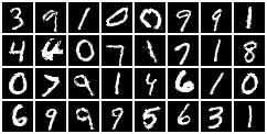
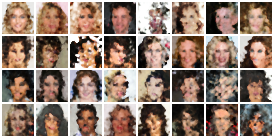
Figure 14: Left: Samples from a set discriminator model trained on MNIST. Right: Samples from a set discriminator model trained on CelebAHQ $32\times 32$.

In addition to our experimental results, we also provide some theoretical evidence that set discriminators may be ill-suited for generative modeling of functions. Specifically, we show that the Lipschitz constant of set discriminators and RFF encodings are typically very large.

B.3 The Lipschitz Constant of Set Discriminators

Several works have shown that limiting the Lipschitz constant (or equivalently the largest gradient norm) of the discriminator is important for stable GAN training (Arjovsky et al., 2017; Gulrajani et al., 2017; Roth et al., 2017; Miyato et al., 2018; Mescheder et al., 2018). This is typically achieved either by penalizing the gradient norm or by explicitly constraining the Lipschitz constant of each layer in the discriminator. Intuitively, this ensures that the gradients of the discriminator with respect to its input do not grow too large and hence that gradients with respect to the weights of the generator do not grow too large either (which can lead to unstable training). In the following subsections, we show that the Lipschitz constant of set discriminators and specifically the Lipschitz constant of RFF encodings are large in most realistic settings.

B.3.1 Architecture

Proposition 1.

The Lipschitz constant of the set discriminator $D$ is bounded by

$$\text{Lip}(D)\leq\text{Lip}(\rho)\text{Lip}(\varphi)\sqrt{\text{Lip}(\gamma_{x})^{2}+\text{Lip}(\gamma_{y})^{2}}$$

See Section C for a proof. In the case where the RFF encoding is fixed, imposing gradient penalties on $D$ would therefore reduce the Lipschitz constant of $\rho$ and $\varphi$ but not of $\gamma_{x}$ and $\gamma_{y}$. If the RFF encoding is learned, its Lipschitz constant could also be penalized. However, as shown in Tancik et al. (2020), learning high frequency functions typically requires large frequencies in the matrix $B$. We show in the following section that the Lipschitz constant of $\gamma$ is directly proportional to the spectral norm of $B$.

B.3.2 Lipschitz Constant of Random Fourier Features

Proposition 2.

The Lipschitz constant of $\gamma(\mathbf{x})$ is bounded by

$$\text{Lip}(\gamma)\leq\sqrt{8}\pi\|B\|$$

See Section C for a proof. There is therefore a fundamental tradeoff between how much high frequency detail the discriminator can learn (requiring a large Lipschitz constant) and its training stability (requiring a low Lipschitz constant). In practice, for the settings we used in this paper, the spectral norm of $B$ is on the order of 100s, which is too large for stable GAN training.

Appendix C PROOFS

C.1 Prerequisites

We denote by $\|\cdot\|_{2}$ the $\ell_{2}$ norm for vectors and by $\|\cdot\|$ the spectral norm for matrices (i.e. the matrix norm induced by the $\ell_{2}$ norm). The spectral norm is defined as

$$\|A\|=\sup_{\|\mathbf{x}\|_{2}=1}\|A\mathbf{x}\|_{2}=\sigma_{\max}(A)=\sqrt{\lambda_{\max}(A^{T}A)}$$

where $\sigma_{\max}$ denotes the largest singular value and $\lambda_{\max}$ the largest eigenvalue.

For a function $f:\mathbb{R}^{n}\to\mathbb{R}^{m}$, the Lipschitz constant $\text{Lip}(f)$ (if it exists) is defined as the largest value $L$ such that

$$\|f(\mathbf{x}_{1})-f(\mathbf{x}_{2})\|_{2}\leq L\|\mathbf{x}_{1}-\mathbf{x}_{2}\|_{2}$$

for all $\mathbf{x}_{1},\mathbf{x}_{2}$. The Lipschitz constant is equivalently defined for differentiable functions as

$$\text{Lip}(f)=\sup_{\mathbf{x}}\|\nabla f(\mathbf{x})\|.$$

Note that when composing two functions $f$ and $g$ we have

$$\text{Lip}(f\circ g)\leq\text{Lip}(f)\text{Lip}(g).$$

We will also make use of the following lemmas.

C.1.1 Spectral Norm of Concatenation

Lemma 1.

Let $A\in\mathbb{R}^{n\times d}$ and $B\in\mathbb{R}^{m\times d}$ be two matrices and denote by $\begin{pmatrix}A\\ B\end{pmatrix}$ their rowwise concatenation. Then we have the following inequality in the spectral norm

$$\left\|\begin{pmatrix}A\\ B\end{pmatrix}\right\|\leq\sqrt{\|A\|^{2}+\|B\|^{2}}.$$

Proof.

$$\left\|\begin{pmatrix}A\\ B\end{pmatrix}\right\|^{2} =\lambda_{\max}\left(\begin{pmatrix}A\\ B\end{pmatrix}^{T}\begin{pmatrix}A\\ B\end{pmatrix}\right)$$

$$=\lambda_{\max}(A^{T}A+B^{T}B)$$

$$\leq\lambda_{\max}(A^{T}A)+\lambda_{\max}(B^{T}B)$$

$$=\|A\|^{2}+\|B\|^{2},$$

where we used the definition of the spectral norm in the first line and Weyl’s inequality for symmetric matrices in the third line.

C.1.2 Inequality for $\ell_{1}$ and $\ell_{2}$ Norm

Lemma 2.

Let $\mathbf{x}_{i}\in\mathbb{R}^{d}$ for $i=1,\dots,n$. Then

$$\sum_{i=1}^{n}\|\mathbf{x}_{i}\|_{2}\leq\sqrt{n}\|(\mathbf{x}_{1},\dots,\mathbf{x}_{n})\|_{2}.$$

Proof.

$$\sum_{i=1}^{n}\|\mathbf{x}_{i}\|_{2} =\sum_{i=1}^{n}\|\mathbf{x}_{i}\|_{2}\cdot 1$$

$$\leq\left(\sum_{i=1}^{n}\|\mathbf{x}_{i}\|^{2}_{2}\right)^{\frac{1}{2}}\left(\sum_{i=1}^{n}1^{2}\right)^{\frac{1}{2}}$$

$$=\sqrt{n}\|(\mathbf{x}_{1},\dots,\mathbf{x}_{n})\|_{2},$$

where we used Cauchy-Schwarz in the second line. Note that this is an extension of the well-known inequality $\|\mathbf{x}\|_{1}\leq\sqrt{n}\|\mathbf{x}\|_{2}$ to the case where each component of the vector $\mathbf{x}$ is the $\ell_{2}$ norm of another vector.

C.1.3 Lipschitz Constant of Sum of Identical Functions

Lemma 3.

Let $\mathbf{x}_{i}\in\mathbb{R}^{d}$ for $i=1,\dots,n$ and let $f$ be a function with Lipschitz constant $\text{Lip}(f)$. Define $g(\mathbf{x}_{1},\dots,\mathbf{x}_{n})=\sum_{i=1}^{n}f(\mathbf{x}_{i})$. Then

$$\text{Lip}(g)\leq\sqrt{n}\text{Lip}(f).$$

Proof.

$$\|g(\mathbf{x}_{1},\dots,\mathbf{x}_{n})-g(\mathbf{y}_{1},...,\mathbf{y}_{n})\|_{2} =\left\|\sum_{i=1}^{n}(f(\mathbf{x}_{i})-f(\mathbf{y}_{i}))\right\|_{2}$$

$$\leq\sum_{i=1}^{n}\|f(\mathbf{x}_{i})-f(\mathbf{y}_{i})\|_{2}$$

$$\leq\text{Lip}(f)\sum_{i=1}^{n}\|\mathbf{x}_{i}-\mathbf{y}_{i}\|_{2}$$

$$\leq\sqrt{n}\text{Lip}(f)\left\|\begin{pmatrix}\mathbf{x}_{1}\\ \vdots\\ \mathbf{x}_{n}\end{pmatrix}-\begin{pmatrix}\mathbf{y}_{1}\\ \vdots\\ \mathbf{y}_{n}\end{pmatrix}\right\|_{2}.$$

Where we used the triangle inequality for norms in the second line, the definition of Lipschitz constants in the second line and Lemma 2 in the third line.

C.1.4 Lipschitz Constant of Concatenation

Lemma 4.

Let $g:\mathbb{R}^{n}\to\mathbb{R}^{m}$ and $h:\mathbb{R}^{p}\to\mathbb{R}^{q}$ be functions with Lipschitz constant $\text{Lip}(g)$ and $\text{Lip}(h)$ respectively. Define $f:\mathbb{R}^{n+p}\to\mathbb{R}^{m+q}$ as the concatenation of $g$ and $h$, that is $f(\mathbf{x},\mathbf{y})=(g(\mathbf{x}),h(\mathbf{y}))$. Then

$$\text{Lip}(f)\leq\sqrt{\text{Lip}(g)^{2}+\text{Lip}(h)^{2}}.$$

Proof.

$$\|f(\mathbf{x}_{1},\mathbf{y}_{1})-f(\mathbf{x}_{2},\mathbf{y}_{2})\|^{2}_{2} =\left\|\begin{pmatrix}g(\mathbf{x}_{1})-g(\mathbf{x}_{2})\\ h(\mathbf{y}_{1})-h(\mathbf{y}_{2})\end{pmatrix}\right\|^{2}_{2}$$

$$=\|g(\mathbf{x}_{1})-g(\mathbf{x}_{2})\|^{2}_{2}+\|h(\mathbf{y}_{1})-h(\mathbf{y}_{2})\|^{2}_{2}$$

$$\leq\text{Lip}(g)^{2}\|\mathbf{x}_{1}-\mathbf{x}_{2}\|^{2}_{2}+\text{Lip}(h)^{2}\|\mathbf{y}_{1}-\mathbf{y}_{2}\|^{2}_{2}$$

$$\leq\text{Lip}(g)^{2}(\|\mathbf{x}_{1}-\mathbf{x}_{2}\|^{2}_{2}+\|\mathbf{y}_{1}-\mathbf{y}_{2}\|^{2}_{2})+\text{Lip}(h)^{2}(\|\mathbf{x}_{1}-\mathbf{x}_{2}\|^{2}_{2}+\|\mathbf{y}_{1}-\mathbf{y}_{2}\|^{2}_{2})$$

$$=(\text{Lip}(g)^{2}+\text{Lip}(h)^{2})\left\|\begin{pmatrix}\mathbf{x}_{1}-\mathbf{x}_{2}\\ \mathbf{y}_{1}-\mathbf{y}_{2}\end{pmatrix}\right\|^{2}_{2}$$

where we used the definition of the $\ell_{2}$ norm in the second and last line.

C.2 Lipschitz Constant of Fourier Feature Encoding

We define the random Fourier feature encoding $\gamma:\mathbb{R}^{d}\to\mathbb{R}^{2m}$ as

$$\gamma(\mathbf{x})=\begin{pmatrix}\cos(2\pi B\mathbf{x})\\ \sin(2\pi B\mathbf{x})\end{pmatrix}$$

where $B\in\mathbb{R}^{m\times d}$.

Proposition 3.

The Lipschitz constant of $\gamma(\mathbf{x})$ is bounded by

$$\text{Lip}(\gamma)\leq\sqrt{8}\pi\|B\|.$$

Proof. Define $\mathbf{u}(\mathbf{x})=\cos(2\pi B\mathbf{x})$ and $\mathbf{v}(\mathbf{x})=\sin(2\pi B\mathbf{x})$. By definition of the Lipschitz constant and applying Lemma 1 we have

$$\text{Lip}(\gamma) =\sup_{\mathbf{x}}\|\nabla\gamma(\mathbf{x})\|$$

$$=\sup_{\mathbf{x}}\left\|\begin{pmatrix}\nabla\cos(2\pi B\mathbf{x})\\ \nabla\sin(2\pi B\mathbf{x})\end{pmatrix}\right\|$$

$$=\sup_{\mathbf{x}}\left\|\begin{pmatrix}\nabla\mathbf{u}(\mathbf{x})\\ \nabla\mathbf{v}(\mathbf{x})\end{pmatrix}\right\|$$

$$\leq\sup_{\mathbf{x}}\sqrt{\|\nabla\mathbf{u}(\mathbf{x})\|^{2}+\|\nabla\mathbf{v}(\mathbf{x})\|^{2}}$$

$$\leq\sqrt{\sup_{\mathbf{x}}\|\nabla\mathbf{u}(\mathbf{x})\|^{2}+\sup_{\mathbf{x}}\|\nabla\mathbf{v}(\mathbf{x})\|^{2}}.$$

The derivative of $\mathbf{u}$ is given by

$$(\nabla\mathbf{u}(\mathbf{x}))_{ij} =\frac{\partial u_{i}({\mathbf{x}})}{\partial x_{j}}$$

$$=\frac{\partial}{\partial x_{j}}\cos(2\pi\mathbf{b}_{i}^{T}\mathbf{x})$$

$$=-2\pi b_{ij}\sin(2\pi\mathbf{b}_{i}^{T}\mathbf{x})$$

$$=-2\pi b_{ij}v_{i}(\mathbf{x}),$$

where $\mathbf{b}_{i}$ corresponds to the ith row of $B$. We can write this more compactly as $\nabla\mathbf{u}(\mathbf{x})=-2\pi\text{diag}(\mathbf{v}(\mathbf{x}))B$. A similar calculation for $\mathbf{v}(\mathbf{x})$ shows that $\nabla\mathbf{v}(\mathbf{x})=2\pi\text{diag}(\mathbf{u}(\mathbf{x}))B$.

All that remains is then to calculate the norms $\|\nabla\mathbf{u}(\mathbf{x})\|$ and $\|\nabla\mathbf{v}(\mathbf{x})\|$. Using submultiplicativity of the spectral norm we have

$$\sup_{\mathbf{x}}\|\nabla\mathbf{u}(\mathbf{x})\| =\sup_{\mathbf{x}}2\pi\|\text{diag}(\mathbf{v}(\mathbf{x}))B\|$$

$$\leq\sup_{\mathbf{x}}2\pi\|\text{diag}(\mathbf{v}(\mathbf{x}))\|\|B\|$$

$$=2\pi\|B\|,$$

where we used the fact that the spectral norm of diagonal matrix is equal to its largest entry and that $|v_{i}(\mathbf{x})|\leq 1$ for all $i$. Similar reasoning gives $\sup_{\mathbf{x}}\|\nabla\mathbf{u}(\mathbf{x})\|=2\pi\|B\|$. Finally we obtain

$$\text{Lip}(\gamma) \leq\sqrt{\sup_{\mathbf{x}}\|\nabla\mathbf{u}(\mathbf{x})\|^{2}+\sup_{\mathbf{x}}\|\nabla\mathbf{v}(\mathbf{x})\|^{2}}$$

$$\leq\sqrt{(2\pi\|B\|)^{2}+(2\pi\|B\|)^{2}}$$

$$=\sqrt{8}\pi\|B\|.$$

C.3 Lipschitz Constant of Set Discriminator

The set discriminator $D:\mathbb{R}^{n\times(d+k)}\to[0,1]$ is defined by

$$D(\mathbf{s})=\rho\left(\frac{1}{\sqrt{n}}\sum_{i=1}^{n}\varphi(\gamma_{x}(\mathbf{x}_{i}),\gamma_{y}(\mathbf{y}_{i}))\right),$$

where $\mathbf{s}=\{(\mathbf{x}_{i},\mathbf{y}_{i})\}_{i=1}^{n}\in\mathbb{R}^{n\times(d+k)}$ is treated as a fixed vector and each $\mathbf{x}_{i}\in\mathbb{R}^{d}$ and $\mathbf{y}_{i}\in\mathbb{R}^{k}$. The Fourier feature encodings for $\mathbf{x}_{i}$ and $\mathbf{y}_{i}$ are given by functions $\gamma_{x}:\mathbb{R}^{d}\to\mathbb{R}^{2m_{x}}$ and $\gamma_{y}:\mathbb{R}^{k}\to\mathbb{R}^{2m_{y}}$ respectively. The function $\varphi:\mathbb{R}^{2(m_{x}+m_{y})}\to\mathbb{R}^{p}$ maps coordinates and features to an encoding of dimension $p$. Finally $\rho:\mathbb{R}^{p}\to[0,1]$ maps the encoding to the probability of the sample being real.

Proposition 4.

The Lipschitz constant of the set discriminator $D$ is bounded by

$$\text{Lip}(D)\leq\text{Lip}(\rho)\text{Lip}(\varphi)\sqrt{\text{Lip}(\gamma_{x})^{2}+\text{Lip}(\gamma_{y})^{2}}.$$

Proof. Write

$$D(\mathbf{s}) =\rho\left(\frac{1}{\sqrt{n}}\sum_{i=1}^{n}\varphi(\gamma_{x}(\mathbf{x}_{i}),\gamma_{y}(\mathbf{y}_{i}))\right)$$

$$=\rho(\eta(\mathbf{s}))$$

where $\eta(\mathbf{s})=\frac{1}{\sqrt{n}}\sum_{i=1}^{n}\varphi(\gamma_{x}(\mathbf{x}_{i}),\gamma_{y}(\mathbf{y}_{i}))$. Then we have

$$\text{Lip}(D)\leq\text{Lip}(\rho)\text{Lip}(\eta).$$

We can further write

$$\eta(\mathbf{s}) =\frac{1}{\sqrt{n}}\sum_{i=1}^{n}\varphi(\gamma_{x}(\mathbf{x}_{i}),\gamma_{y}(\mathbf{y}_{i}))$$

$$=\frac{1}{\sqrt{n}}\sum_{i=1}^{n}\theta(\mathbf{s}_{i}),$$

where $\mathbf{s}_{i}=(\mathbf{x}_{i},\mathbf{y}_{i})$ and $\theta(\mathbf{s}_{i})=\varphi(\gamma_{x}(\mathbf{x}_{i}),\gamma_{y}(\mathbf{y}_{i}))$. By Lemma 3 we have

$$\text{Lip}(\eta)\leq\frac{1}{\sqrt{n}}\sqrt{n}\text{Lip}(\theta)=\text{Lip}(\theta).$$

We can then write

$$\theta(\mathbf{s}_{i}) =\varphi(\gamma_{x}(\mathbf{x}_{i}),\gamma_{y}(\mathbf{y}_{i}))$$

$$=\varphi(\psi(\mathbf{s}_{i}))$$

where $\psi(\mathbf{s}_{i})=(\gamma_{x}(\mathbf{x}_{i}),\gamma_{y}(\mathbf{y}_{i}))$. We then have, using Lemma 4

$$\text{Lip}(\theta)\leq\text{Lip}(\varphi)\text{Lip}(\psi)\leq\text{Lip}(\varphi)\sqrt{\text{Lip}(\gamma_{x})^{2}+\text{Lip}(\gamma_{y})^{2}}.$$

Putting everything together we finally obtain

$$\text{Lip}(D)\leq\text{Lip}(\rho)\text{Lip}(\varphi)\sqrt{\text{Lip}(\gamma_{x})+\text{Lip}(\gamma_{y})}.$$

Appendix D FAILURE EXAMPLES

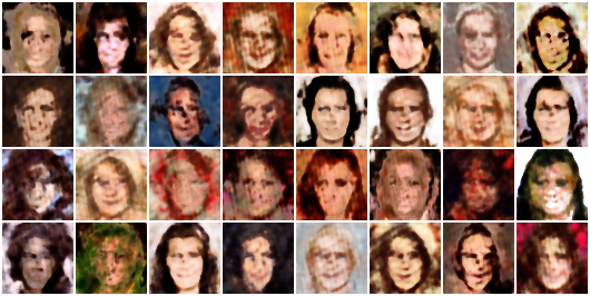
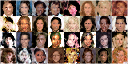
Figure 15: Left: Samples from model trained on CelebAHQ $64\times 64$ using $K=2048$ pixels (50%). Right: Samples from model trained using $K=3072$ pixels (75%).

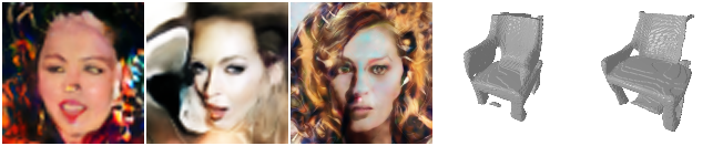
Figure 16: Selected samples highlighting failure modes of our model, including generation of unrealistic and incoherent samples.

Appendix E ADDITIONAL RESULTS

E.1 Additional Evaluation on ERA5 Climate Data

As metrics like FID are not applicable to the ERA5 data, we provide additional experimental results to strengthen the evaluation of GASP on this data modality. Figure 22 shows comparisons between samples from GASP and the training data. As can be seen, the samples produced from our model are largely indistinguishable from real samples. To ensure the model has not memorized samples from the training set, but rather has learned a smooth manifold of the data, we show examples of latent interpolations in Figure 23. Finally, Figure 24 shows a histogram comparing the distribution of temperatures in the test set and the distribution of temperatures obtained from GASP samples.

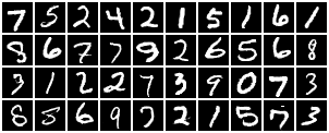
Figure 17: Additional MNIST samples.

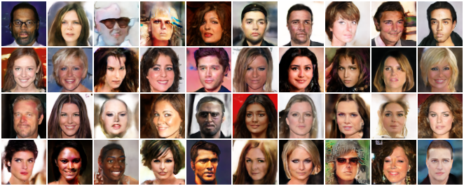
Figure 18: Additional CelebAHQ $64\times 64$ samples.

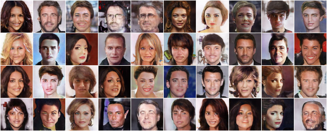
Figure 19: Additional CelebAHQ $128\times 128$ samples.

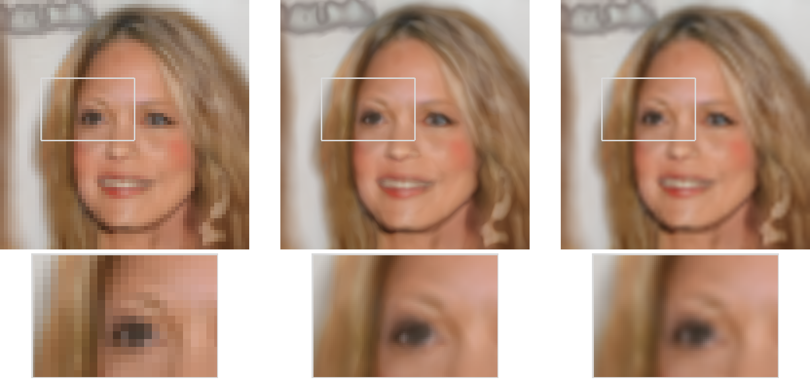
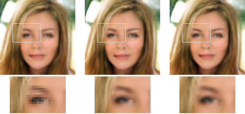
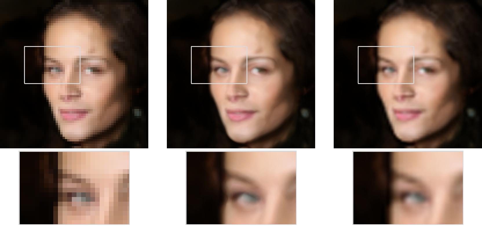
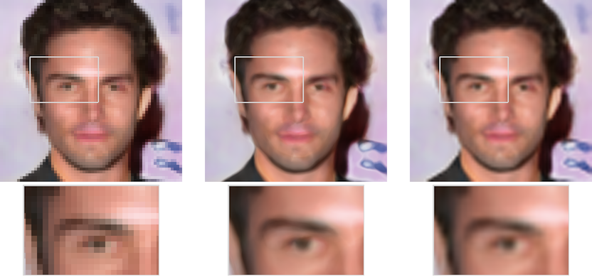
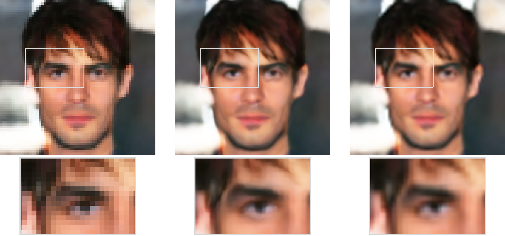
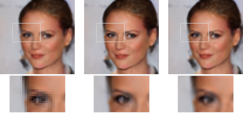
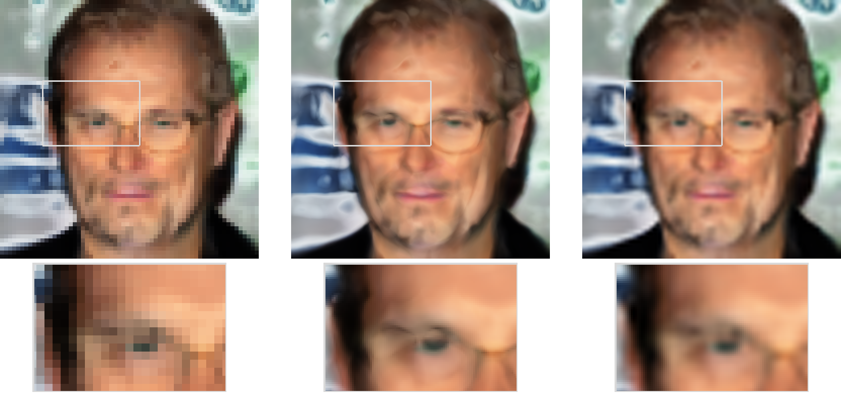
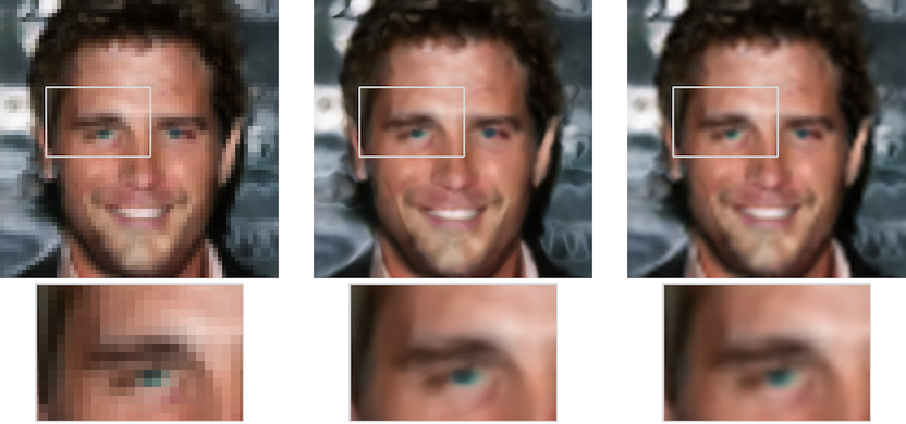
Figure 20: Additional superresolution samples. Left column shows superresolution from $64\times 64\to 256\times 256$ and right column shows superresolution from $64\times 64\to 512\times 512$

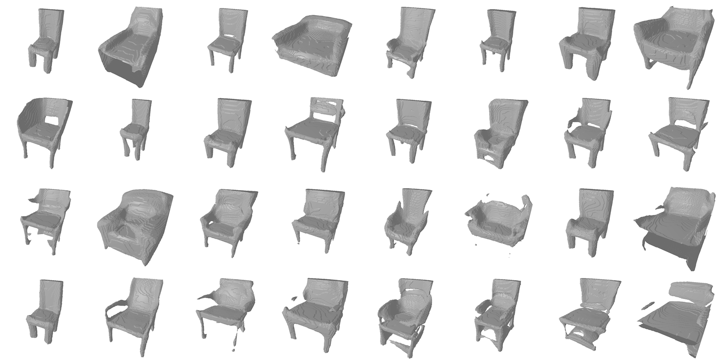
Figure 21: Additional Shapenet chairs samples.

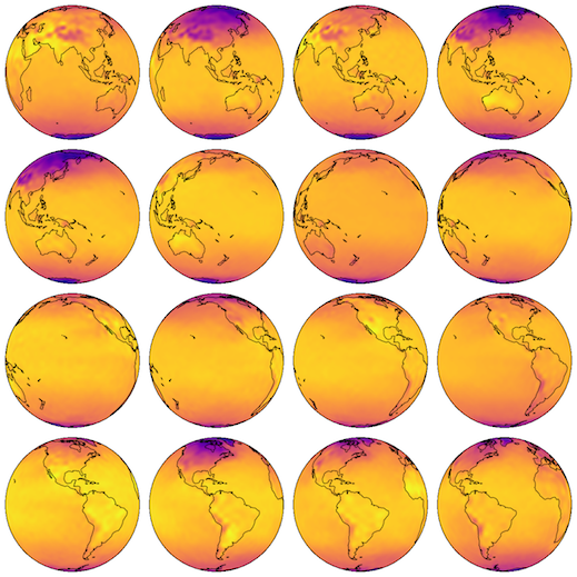
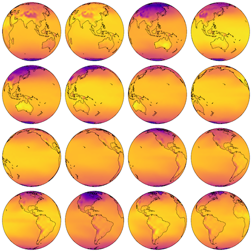
Figure 22: Random samples from GASP (left) and the training data (right).

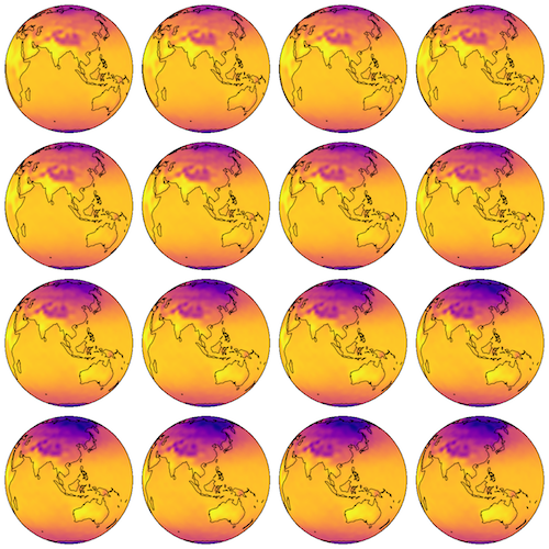
Figure 23: Latent (function space) interpolation between two random samples from GASP. As can be seen the the model has learned a smooth latent space for the data.

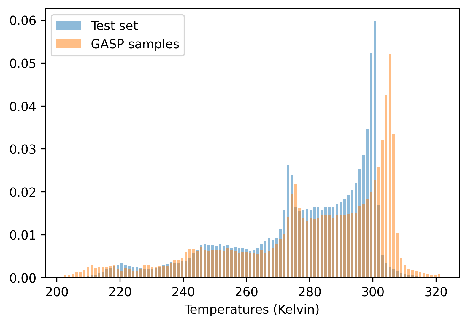
Figure 24: Distribution of temperatures in test set and from GASP samples. As can be seen, the distribution of temperatures from GASP roughly matches the distribution in the test set.

References

- Anokhin et al. (2021) Ivan Anokhin, Kirill Demochkin, Taras Khakhulin, Gleb Sterkin, Victor Lempitsky, and Denis Korzhenkov. Image generators with conditionally-independent pixel synthesis. In Proceedings of the IEEE/CVF Conference on Computer Vision and Pattern Recognition, pages 14278–14287, 2021.
- Arjovsky et al. (2017) Martin Arjovsky, Soumith Chintala, and Léon Bottou. Wasserstein generative adversarial networks. In International Conference on Machine Learning, pages 214–223, 2017.
- Atzmon and Lipman (2020) Matan Atzmon and Yaron Lipman. Sal: Sign agnostic learning of shapes from raw data. In Proceedings of the IEEE/CVF Conference on Computer Vision and Pattern Recognition, pages 2565–2574, 2020.
- Atzmon and Lipman (2021) Matan Atzmon and Yaron Lipman. SALD: Sign agnostic learning with derivatives. In International Conference on Learning Representations, 2021.
- Bond-Taylor and Willcocks (2021) Sam Bond-Taylor and Chris G Willcocks. Gradient origin networks. In International Conference on Learning Representations, 2021.
- Borovitskiy et al. (2021) Viacheslav Borovitskiy, Iskander Azangulov, Alexander Terenin, Peter Mostowsky, Marc Deisenroth, and Nicolas Durrande. Matérn Gaussian processes on graphs. In International Conference on Artificial Intelligence and Statistics, pages 2593–2601, 2021.
- Brock et al. (2019) Andrew Brock, Jeff Donahue, and Karen Simonyan. Large scale gan training for high fidelity natural image synthesis. In International Conference on Learning Representations, 2019.
- Cai et al. (2020) Ruojin Cai, Guandao Yang, Hadar Averbuch-Elor, Zekun Hao, Serge Belongie, Noah Snavely, and Bharath Hariharan. Learning gradient fields for shape generation. In Computer Vision–ECCV 2020: 16th European Conference, Glasgow, UK, August 23–28, 2020, Proceedings, Part III 16, pages 364–381. Springer, 2020.
- Chan et al. (2021) Eric R Chan, Marco Monteiro, Petr Kellnhofer, Jiajun Wu, and Gordon Wetzstein. pi-GAN: Periodic implicit generative adversarial networks for 3d-aware image synthesis. In Proceedings of the IEEE/CVF Conference on Computer Vision and Pattern Recognition, pages 5799–5809, 2021.
- Chang et al. (2015) Angel X Chang, Thomas Funkhouser, Leonidas Guibas, Pat Hanrahan, Qixing Huang, Zimo Li, Silvio Savarese, Manolis Savva, Shuran Song, Hao Su, et al. Shapenet: An information-rich 3d model repository. arXiv preprint arXiv:1512.03012, 2015.
- Chen et al. (2021) Yinbo Chen, Sifei Liu, and Xiaolong Wang. Learning continuous image representation with local implicit image function. In Proceedings of the IEEE/CVF Conference on Computer Vision and Pattern Recognition, pages 8628–8638, 2021.
- Chen and Zhang (2019) Zhiqin Chen and Hao Zhang. Learning implicit fields for generative shape modeling. In Proceedings of the IEEE/CVF Conference on Computer Vision and Pattern Recognition, pages 5939–5948, 2019.
- Choy et al. (2016) Christopher B Choy, Danfei Xu, JunYoung Gwak, Kevin Chen, and Silvio Savarese. 3d-r2n2: A unified approach for single and multi-view 3d object reconstruction. In European Conference on Computer Vision, pages 628–644. Springer, 2016.
- Cohen et al. (2018) Taco S Cohen, Mario Geiger, Jonas Köhler, and Max Welling. Spherical cnns. In International Conference on Learning Representations, 2018.
- Dupont et al. (2018) Emilien Dupont, Tuanfeng Zhang, Peter Tilke, Lin Liang, and William Bailey. Generating realistic geology conditioned on physical measurements with generative adversarial networks. arXiv preprint arXiv:1802.03065, 2018.
- Esteves et al. (2018) Carlos Esteves, Christine Allen-Blanchette, Ameesh Makadia, and Kostas Daniilidis. Learning SO(3) equivariant representations with spherical CNNs. In Proceedings of the European Conference on Computer Vision (ECCV), pages 52–68, 2018.
- Garnelo et al. (2018a) Marta Garnelo, Dan Rosenbaum, Christopher Maddison, Tiago Ramalho, David Saxton, Murray Shanahan, Yee Whye Teh, Danilo Rezende, and SM Ali Eslami. Conditional neural processes. In International Conference on Machine Learning, pages 1704–1713. PMLR, 2018a.
- Garnelo et al. (2018b) Marta Garnelo, Jonathan Schwarz, Dan Rosenbaum, Fabio Viola, Danilo J Rezende, SM Eslami, and Yee Whye Teh. Neural processes. arXiv preprint arXiv:1807.01622, 2018b.
- Goodfellow et al. (2014) Ian J Goodfellow, Jean Pouget-Abadie, Mehdi Mirza, Bing Xu, David Warde-Farley, Sherjil Ozair, Aaron Courville, and Yoshua Bengio. Generative adversarial networks. In Advances in Neural Information Processing Systems, 2014.
- Gordon et al. (2019) Jonathan Gordon, Wessel P Bruinsma, Andrew YK Foong, James Requeima, Yann Dubois, and Richard E Turner. Convolutional conditional neural processes. In International Conference on Learning Representations, 2019.
- Gropp et al. (2020) Amos Gropp, Lior Yariv, Niv Haim, Matan Atzmon, and Yaron Lipman. Implicit geometric regularization for learning shapes. In International Conference on Machine Learning, pages 3789–3799. PMLR, 2020.
- Gulrajani et al. (2017) Ishaan Gulrajani, Faruk Ahmed, Martin Arjovsky, Vincent Dumoulin, and Aaron C Courville. Improved training of Wasserstein gans. In Advances in Neural Information Processing Systems, pages 5767–5777, 2017.
- Ha (2016) David Ha. Generating large images from latent vectors. blog.otoro.net, 2016. URL https://blog.otoro.net/2016/04/01/generating-large-images-from-latent-vectors/.
- Ha et al. (2017) David Ha, Andrew Dai, and Quoc V Le. HyperNetworks. International Conference on Learning Representations, 2017.
- Hersbach et al. (2019) H. Hersbach, B. Bell, P. Berrisford, G. Biavati, A. Horányi, J. Muñoz Sabater, J. Nicolas, C. Peubey, R. Radu, I. Rozum, D. Schepers, A. Simmons, C. Soci, D. Dee, and J-N. Thépaut. ERA5 monthly averaged data on single levels from 1979 to present. Copernicus Climate Change Service (C3S) Climate Data Store (CDS). https://cds.climate.copernicus.eu/cdsapp#!/dataset/reanalysis-era5-single-levels-monthly-means (Accessed 27-09-2021), 2019.
- Ioffe and Szegedy (2015) Sergey Ioffe and Christian Szegedy. Batch normalization: Accelerating deep network training by reducing internal covariate shift. In International Conference on Machine Learning, pages 448–456. PMLR, 2015.
- Jean et al. (2016) Neal Jean, Marshall Burke, Michael Xie, W Matthew Davis, David B Lobell, and Stefano Ermon. Combining satellite imagery and machine learning to predict poverty. Science, 353(6301):790–794, 2016.
- Jensen et al. (2020) Kristopher Jensen, Ta-Chu Kao, Marco Tripodi, and Guillaume Hennequin. Manifold GPLVMs for discovering non-euclidean latent structure in neural data. Advances in Neural Information Processing Systems, 2020.
- Jiang et al. (2020) Chiyu Jiang, Avneesh Sud, Ameesh Makadia, Jingwei Huang, Matthias Nießner, Thomas Funkhouser, et al. Local implicit grid representations for 3d scenes. In Proceedings of the IEEE/CVF Conference on Computer Vision and Pattern Recognition, pages 6001–6010, 2020.
- Johnson et al. (2019) Jeff Johnson, Matthijs Douze, and Hervé Jégou. Billion-scale similarity search with GPUs. IEEE Transactions on Big Data, 2019.
- Karras et al. (2018) Tero Karras, Timo Aila, Samuli Laine, and Jaakko Lehtinen. Progressive growing of gans for improved quality, stability, and variation. In International Conference on Learning Representations, 2018.
- Karras et al. (2019) Tero Karras, Samuli Laine, and Timo Aila. A style-based generator architecture for generative adversarial networks. In Proceedings of the IEEE/CVF Conference on Computer Vision and Pattern Recognition, pages 4401–4410, 2019.
- Kim et al. (2019) Hyunjik Kim, Andriy Mnih, Jonathan Schwarz, Marta Garnelo, Ali Eslami, Dan Rosenbaum, Oriol Vinyals, and Yee Whye Teh. Attentive neural processes. In International Conference on Learning Representations, 2019.
- Kingma and Welling (2014) Diederik P Kingma and Max Welling. Auto-encoding variational Bayes. In International Conference on Learning Representations, 2014.
- Kleineberg et al. (2020) Marian Kleineberg, Matthias Fey, and Frank Weichert. Adversarial generation of continuous implicit shape representations. In Eurographics - Short Papers, 2020.
- Lee et al. (2019) Juho Lee, Yoonho Lee, Jungtaek Kim, Adam Kosiorek, Seungjin Choi, and Yee Whye Teh. Set transformer: A framework for attention-based permutation-invariant neural networks. In International Conference on Machine Learning, pages 3744–3753. PMLR, 2019.
- Li et al. (2018) Yangyan Li, Rui Bu, Mingchao Sun, Wei Wu, Xinhan Di, and Baoquan Chen. PointCNN: Convolution on x-transformed points. Advances in Neural Information Processing Systems, 31:820–830, 2018.
- Lin et al. (2019) Chieh Hubert Lin, Chia-Che Chang, Yu-Sheng Chen, Da-Cheng Juan, Wei Wei, and Hwann-Tzong Chen. Coco-gan: Generation by parts via conditional coordinating. In Proceedings of the IEEE/CVF International Conference on Computer Vision, pages 4512–4521, 2019.
- Lorensen and Cline (1987) William E Lorensen and Harvey E Cline. Marching cubes: A high resolution 3d surface construction algorithm. ACM Siggraph Computer Graphics, 21(4):163–169, 1987.
- Mescheder et al. (2018) Lars Mescheder, Andreas Geiger, and Sebastian Nowozin. Which training methods for gans do actually converge? In International Conference on Machine learning, pages 3481–3490, 2018.
- Mescheder et al. (2019) Lars Mescheder, Michael Oechsle, Michael Niemeyer, Sebastian Nowozin, and Andreas Geiger. Occupancy networks: Learning 3d reconstruction in function space. In Proceedings of the IEEE/CVF Conference on Computer Vision and Pattern Recognition, pages 4460–4470, 2019.
- Mescheder (2020) Lars Morten Mescheder. Stability and Expressiveness of Deep Generative Models. PhD thesis, Universität Tübingen, 2020.
- Mildenhall et al. (2020) Ben Mildenhall, Pratul P Srinivasan, Matthew Tancik, Jonathan T Barron, Ravi Ramamoorthi, and Ren Ng. Nerf: Representing scenes as neural radiance fields for view synthesis. In European Conference on Computer Vision, pages 405–421, 2020.
- Miyato et al. (2018) Takeru Miyato, Toshiki Kataoka, Masanori Koyama, and Yuichi Yoshida. Spectral normalization for generative adversarial networks. In International Conference on Learning Representations, 2018.
- Niemeyer and Geiger (2021) Michael Niemeyer and Andreas Geiger. GIRAFFE: Representing scenes as compositional generative neural feature fields. In Proceedings of the IEEE/CVF Conference on Computer Vision and Pattern Recognition, pages 11453–11464, 2021.
- Niemeyer et al. (2019) Michael Niemeyer, Lars Mescheder, Michael Oechsle, and Andreas Geiger. Occupancy flow: 4d reconstruction by learning particle dynamics. In Proceedings of the IEEE/CVF International Conference on Computer Vision, pages 5379–5389, 2019.
- Niemeyer et al. (2020) Michael Niemeyer, Lars Mescheder, Michael Oechsle, and Andreas Geiger. Differentiable volumetric rendering: Learning implicit 3d representations without 3d supervision. In Proc. IEEE Conf. on Computer Vision and Pattern Recognition (CVPR), 2020.
- Park et al. (2019) Jeong Joon Park, Peter Florence, Julian Straub, Richard Newcombe, and Steven Lovegrove. Deepsdf: Learning continuous signed distance functions for shape representation. In Proceedings of the IEEE Conference on Computer Vision and Pattern Recognition, pages 165–174, 2019.
- Paszke et al. (2019) Adam Paszke, Sam Gross, Francisco Massa, Adam Lerer, James Bradbury, Gregory Chanan, Trevor Killeen, Zeming Lin, Natalia Gimelshein, Luca Antiga, et al. Pytorch: An imperative style, high-performance deep learning library. Advances in Neural Information Processing Systems, 32:8026–8037, 2019.
- Pumarola et al. (2021) Albert Pumarola, Enric Corona, Gerard Pons-Moll, and Francesc Moreno-Noguer. D-nerf: Neural radiance fields for dynamic scenes. In Proceedings of the IEEE/CVF Conference on Computer Vision and Pattern Recognition, pages 10318–10327, 2021.
- Qi et al. (2017) Charles R Qi, Hao Su, Kaichun Mo, and Leonidas J Guibas. Pointnet: Deep learning on point sets for 3d classification and segmentation. In Proceedings of the IEEE conference on Computer Vision and Pattern Eecognition, pages 652–660, 2017.
- Radford et al. (2015) Alec Radford, Luke Metz, and Soumith Chintala. Unsupervised representation learning with deep convolutional generative adversarial networks. arXiv preprint arXiv:1511.06434, 2015.
- Ravi et al. (2020) Nikhila Ravi, Jeremy Reizenstein, David Novotny, Taylor Gordon, Wan-Yen Lo, Justin Johnson, and Georgia Gkioxari. Accelerating 3d deep learning with pytorch3d. arXiv preprint arXiv:2007.08501, 2020.
- Rezende et al. (2014) Danilo Jimenez Rezende, Shakir Mohamed, and Daan Wierstra. Stochastic backpropagation and approximate inference in deep generative models. In International Conference on Machine Learning, pages 1278–1286. PMLR, 2014.
- Roth et al. (2017) Kevin Roth, Aurelien Lucchi, Sebastian Nowozin, and Thomas Hofmann. Stabilizing training of generative adversarial networks through regularization. In Advances in Neural Information Processing Systems, pages 2018–2028, 2017.
- Schwarz et al. (2020) Katja Schwarz, Yiyi Liao, Michael Niemeyer, and Andreas Geiger. GRAF: Generative radiance fields for 3d-aware image synthesis. Advances in Neural Information Processing Systems, 33, 2020.
- Seitzer (2020) Maximilian Seitzer. pytorch-fid: FID Score for PyTorch. https://github.com/mseitzer/pytorch-fid, August 2020. Version 0.1.1.
- Sitzmann et al. (2019) Vincent Sitzmann, Michael Zollhöfer, and Gordon Wetzstein. Scene representation networks: Continuous 3d-structure-aware neural scene representations. In Advances in Neural Information Processing Systems, pages 1121–1132, 2019.
- Sitzmann et al. (2020) Vincent Sitzmann, Julien Martel, Alexander Bergman, David Lindell, and Gordon Wetzstein. Implicit neural representations with periodic activation functions. Advances in Neural Information Processing Systems, 33, 2020.
- Skorokhodov et al. (2021) Ivan Skorokhodov, Savva Ignatyev, and Mohamed Elhoseiny. Adversarial generation of continuous images. In Proceedings of the IEEE/CVF Conference on Computer Vision and Pattern Recognition, pages 10753–10764, 2021.
- Sønderby et al. (2020) Casper Kaae Sønderby, Lasse Espeholt, Jonathan Heek, Mostafa Dehghani, Avital Oliver, Tim Salimans, Shreya Agrawal, Jason Hickey, and Nal Kalchbrenner. Metnet: A neural weather model for precipitation forecasting. arXiv preprint arXiv:2003.12140, 2020.
- Spurek et al. (2020) Przemysław Spurek, Sebastian Winczowski, Jacek Tabor, Maciej Zamorski, Maciej Zieba, and Tomasz Trzcinski. Hypernetwork approach to generating point clouds. In International Conference on Machine Learning, pages 9099–9108, 2020.
- Stanley (2007) Kenneth O Stanley. Compositional pattern producing networks: A novel abstraction of development. Genetic programming and evolvable machines, 8(2):131–162, 2007.
- Stelzner et al. (2020) Karl Stelzner, Kristian Kersting, and Adam R Kosiorek. Generative adversarial set transformers. In Workshop on Object-Oriented Learning at ICML, volume 2020, 2020.
- Tancik et al. (2020) Matthew Tancik, Pratul P Srinivasan, Ben Mildenhall, Sara Fridovich-Keil, Nithin Raghavan, Utkarsh Singhal, Ravi Ramamoorthi, Jonathan T Barron, and Ren Ng. Fourier features let networks learn high frequency functions in low dimensional domains. In Advances in Neural Information Processing Systems, 2020.
- Thomas et al. (2019) Hugues Thomas, Charles R Qi, Jean-Emmanuel Deschaud, Beatriz Marcotegui, François Goulette, and Leonidas J Guibas. Kpconv: Flexible and deformable convolution for point clouds. In Proceedings of the IEEE/CVF International Conference on Computer Vision, pages 6411–6420, 2019.
- Wu et al. (2019) Wenxuan Wu, Zhongang Qi, and Li Fuxin. Pointconv: Deep convolutional networks on 3d point clouds. In Proceedings of the IEEE Conference on Computer Vision and Pattern Recognition, pages 9621–9630, 2019.
- Wu et al. (2018) Zhenqin Wu, Bharath Ramsundar, Evan N Feinberg, Joseph Gomes, Caleb Geniesse, Aneesh S Pappu, Karl Leswing, and Vijay Pande. Moleculenet: a benchmark for molecular machine learning. Chemical Science, 9(2):513–530, 2018.
- Yu et al. (2021) Alex Yu, Vickie Ye, Matthew Tancik, and Angjoo Kanazawa. pixelnerf: Neural radiance fields from one or few images. In Proceedings of the IEEE/CVF Conference on Computer Vision and Pattern Recognition, pages 4578–4587, 2021.
- Zaheer et al. (2017) Manzil Zaheer, Satwik Kottur, Siamak Ravanbakhsh, Barnabas Poczos, Russ R Salakhutdinov, and Alexander J Smola. Deep sets. In Advances in Neural Information Processing Systems, pages 3391–3401, 2017.