Quasi-Global Momentum:
Accelerating Decentralized Deep Learning on Heterogeneous Data

Abstract

Decentralized training of deep learning models is a key element for enabling data privacy and on-device learning over networks. In realistic learning scenarios, the presence of heterogeneity across different clients’ local datasets poses an optimization challenge and may severely deteriorate the generalization performance.
In this paper, we investigate and identify the limitation of several decentralized optimization algorithms for different degrees of data heterogeneity. We propose a novel momentum-based method to mitigate this decentralized training difficulty. We show in extensive empirical experiments on various CV/NLP datasets (CIFAR-10, ImageNet, and AG News) and several network topologies (Ring and Social Network) that our method is much more robust to the heterogeneity of clients’ data than other existing methods, by a significant improvement in test performance ($1\%\!-\!20\%$). Our code is publicly available.

1 Introduction

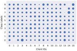
(a) CIFAR-10, $n\!=\!16$, $\alpha=10$.

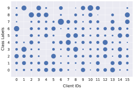
(b) CIFAR-10, $n\!=\!16$, $\alpha=1$.

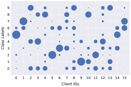
(c) CIFAR-10, $n\!=\!16$, $\alpha=0.1$.

Methods	Ring ($n\!=\!16$)			Social Network ($n\!=\!32$)
	$\alpha=10$	$\alpha=1$	$\alpha=0.1$	$\alpha=10$	$\alpha=1$	$\alpha=0.1$
DSGD	$89.90\pm 0.26$	$88.88\pm 0.26$	$74.55\pm 2.07$	$89.95\pm 0.23$	$88.41\pm 0.27$	$77.56\pm 1.65$
DSGDm-N	$91.47\pm 0.23$	$89.98\pm 0.10$	$77.48\pm 2.67$	$91.17\pm 0.11$	$89.96\pm 0.35$	$80.59\pm 2.32$
QG-DSGDm-N (ours)	$\textbf{91.90}\pm 0.17$	$\textbf{91.28}\pm 0.38$	$\textbf{82.20}\pm 1.27$	$\textbf{91.51}\pm 0.02$	$\textbf{91.00}\pm 0.24$	$\textbf{85.19}\pm 0.98$

Figure 1: Illustrating the challenge of heterogeneous data in decentralized deep learning, for training ResNet-EvoNorm-20 on CIFAR-10. The Dirichlet distribution $\alpha$ values control different non-i.i.d. degrees (Yurochkin et al., 2019; Hsu et al., 2019; He et al., 2020); the smaller $\alpha$ is, the more likely the clients hold examples from only one class. The inline figures illustrate the # of samples per class allocated to each client (indicated by dot sizes), for the case of $\alpha\!=\!10,1,0.1$. The test top-1 accuracy results in the table are averaged over three random seeds, with learning rate tuning for each setting. The performance upper bound (i.e. centralized training without local data re-shuffling) for $n\!=\!16$ and $32$ nodes are $92.95\pm 0.13$ and $92.88\pm 0.07$ respectively. Following prior work, the evaluated DSGD methods maintain local momentum buffer (without synchronization) for each worker; other experimental setup refers to Section 5.1.

Decentralized machine learning methods—allowing communications in a peer-to-peer fashion on an underlying communication network topology (without a central coordinator)—have emerged as an important paradigm in large-scale machine learning (Lian et al., 2017, 2018; Koloskova et al., 2019, 2020b). Decentralized Stochastic Gradient Descent (DSGD) methods offer (1) scalability to large datasets and systems in large data-centers (Lian et al., 2017; Assran et al., 2019; Koloskova et al., 2020a), as well as (2) privacy-preserving learning for the emerging EdgeAI applications (Kairouz et al., 2019; Koloskova et al., 2020a), where the training data remains distributed over a large number of clients (e.g. mobile phones, sensors, or hospitals) and is kept locally (never transmitted during training).

A key challenge—in particular in the second scenario—is the large heterogeneity (non-i.i.d.-ness) in the data present on the different clients (Zhao et al., 2018; Kairouz et al., 2019; Hsieh et al., 2020). Heterogeneous data (e.g. as illustrated in Figure 1) causes very diverse optimization objectives on each client, which results in slow and unstable global convergence, as well as poor generalization performance (shown in the inline table of Figure 1). Addressing these optimization difficulties is essential to realize reliable decentralized deep learning applications. Although such challenges have been theoretically pointed out in (Shi et al., 2015; Lee et al., 2015; Tang et al., 2018b; Koloskova et al., 2020b), the empirical performance of different DSGD methods remains poorly understood. To the best of our knowledge, there currently exists no efficient, effective, and robust optimization algorithm yet for decentralized deep learning on heterogeneous data.

In the meantime, SGD with momentum acceleration (SGDm) remains the current workhorse for the state-of-the-art (SOTA) centralized deep learning training (He et al., 2016; Goyal et al., 2017; He et al., 2019). For decentralized deep learning, the currently used training recipes (i.e. DSGDm) maintain a local momentum buffer on each worker (Assran et al., 2019; Koloskova et al., 2020a; Nadiradze et al., 2020; Singh et al., 2020; Kong et al., 2021) while only communicating the model parameters to the neighbors. However, these attempts in prior work mainly consider homogeneous decentralized data—and there is no evidence that local momentum enhances generalization performance of decentralized deep learning on heterogeneous data.

As our first contribution, we investigate how DSGD and DSGDm are impacted by the degree of data heterogeneity and the choice of the network topology. We find that heterogeneous data hinders the local momentum acceleration in DSGDm. We further show that using a high-quality shared momentum buffer (e.g. synchronizing the momentum buffer globally) improves the optimization and generalization performance of DSGDm. However, such a global communication significantly increases the communication cost and violates the decentralized learning setup.

We instead propose Quasi-Global (QG) momentum, a simple, yet effective, method that mitigates the difficulties for decentralized learning on heterogeneous data. Our approach is based on locally approximating the global optimization direction without introducing extra communication overhead. We demonstrate in extensive empirical results that QG momentum can stabilize the optimization trajectory, and that it can accelerate decentralized learning achieving much better generalization performance under high data heterogeneity than previous methods.

• We systematically examine the behavior of decentralized optimization algorithms on standard deep learning benchmarks for various degrees of data heterogeneity.

• We propose a novel momentum-based decentralized optimization method—QG-DSGDm and QG-DSGDm-N—to stabilize the local optimization. We validate the effectiveness of our method on a spectrum of non-i.i.d. degrees and network topologies—it is much more robust to the data heterogeneity than all other existing methods.

• We rigorously prove the convergence of our scheme.

• We additionally investigate different normalization methods alternative to Batch Normalization (BN) (Ioffe & Szegedy, 2015) in CNNs, due to its particular vulnerable to non-i.i.d. local data and the caused severe quality loss.

2 Related Work

Decentralized Deep Learning. The study of decentralized optimization algorithms dates back to Tsitsiklis (1984), relating to use gossip algorithms (Kempe et al., 2003; Xiao & Boyd, 2004; Boyd et al., 2006) to compute aggregates (find consensus) among clients. In the context of machine learning/deep learning, combining SGD with gossip averaging (Lian et al., 2017, 2018; Assran et al., 2019; Koloskova et al., 2020b) has gained a lot of attention recently for the benefits of computational scalability, communication efficiency, data locality, as well as the favorable leading term in the convergence rate $\smash{\mathcal{O}\big{(}\frac{1}{n\varepsilon^{2}}\big{)}}$ (Lian et al., 2017; Scaman et al., 2017, 2018; Tang et al., 2018b; Koloskova et al., 2019, 2020a, 2020b) which is the same as in centralized mini-batch SGD (Dekel et al., 2012). A weak version of decentralized learning also covers the recent emerging federated learning (FL) setting (Konecnỳ et al., 2016; McMahan et al., 2017; Kairouz et al., 2019; Karimireddy et al., 2020b; Lin et al., 2020b) by using (centralized) star-shaped network topology and local updates. Note that specializing our results to the FL setting is beyond the scope of our work. It is also non-trivial to adapt certain very recent techniques developed in FL for heterogeneous data (Karimireddy et al., 2020b, a; Lin et al., 2020b; Wang et al., 2020a; Das et al., 2020; Haddadpour et al., 2021) to the gossip-based decentralized deep learning.

A line of recent works on decentralized stochastic optimization, like D${}^{2}$/Exact-diffusion (Tang et al., 2018b; Yuan et al., 2020a; Yuan & Alghunaim, 2021), and gradient tracking (Pu & Nedić, 2020; Pan et al., 2020; Lu et al., 2019), proposes different techniques to theoretically eliminate the influence of data heterogeneity between nodes. However, it remains unclear if these theoretically sound methods still endow with superior convergence and generalization properties in deep learning.

Other works focus on improving communication efficiency, from the aspect of communication compression (Tang et al., 2018a; Koloskova et al., 2019, 2020a; Lu & De Sa, 2020; Taheri et al., 2020; Singh et al., 2020; Vogels et al., 2020; Taheri et al., 2020; Nadiradze et al., 2020), less frequent communication through multiple local updates (Hendrikx et al., 2019; Koloskova et al., 2020b; Nadiradze et al., 2020), or better communication topology design (Nedić et al., 2018; Assran et al., 2019; Wang et al., 2019, 2020b; Neglia et al., 2020; Nadiradze et al., 2020; Kong et al., 2021).

Mini-batch SGD with Momentum Acceleration. Momentum is a critical component for training the SOTA deep neural networks (Sutskever et al., 2013; Lucas et al., 2019). Despite various empirical successes, the current theoretical understanding of momentum-based SGD methods remains limited (Bottou et al., 2016). A line of work on the serial (centralized) setting has aimed to develop a convergence analysis for different momentum methods as a special case (Yan et al., 2018; Gitman et al., 2019). However, SGD is known to be optimal in the worst case for stochastic non-convex optimization (Arjevani et al., 2019).
In distributed deep learning, most prior works focus on homogeneous data (especially for numerical evaluations) and incorporate momentum with a locally maintained buffer (which has no synchronization) (Lian et al., 2017; Assran et al., 2019; Lin et al., 2020c, a; Koloskova et al., 2020a; Singh et al., 2020). Yu et al. (2019) propose synchronizing the local momentum buffer periodically for better performance at the cost of doubling the communication. SlowMo (Wang et al., 2020c) instead proposes to periodically perform a slow momentum update on the globally synchronized model parameters (with additional All-Reduce communication cost), for centralized or decentralized methods. Parallel work (Balu et al., 2020) introduces DMSGD for decentralized learning—it constructs the acceleration momentum from the mixture of the local momentum and consensus momentum. Our proposed method has no extra communication overhead and significantly outperforms all existing methods (in Section 5.2).

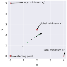
(a) w/o local momentum.

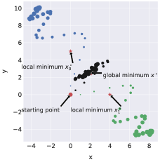
(b) w/ local HeavyBall momentum.

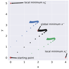
(c) Our scheme.

Figure 2: The ineffectiveness of local momentum acceleration under heterogeneous data setup: the local momentum buffer accumulates “biased” gradients, causing unstable and oscillation behaviors. The size of marker increase proportional to the number of update steps; colors blue and green indicate the local models of two workers (after performing local update), while black color indicates the synchronized global model. Uniform weight averaging is performed after each update step, and the new gradients are computed on the averaged model. We use the common $\beta\!=\!0.9$ in this illustration. For additional results with different $\beta$ values refer to Appendix LABEL:appendix:more_on_2D_illustration.

Batch Normalization in Distributed Learning. Batch Normalization (BN) (Ioffe & Szegedy, 2015) is an indispensable component in deep learning (Santurkar et al., 2018; Luo et al., 2019) and has been employed by default in most SOTA CNNs (He et al., 2016; Huang et al., 2016; Tan & Le, 2019). However, it often fails on distributed deep learning with heterogeneous local data due to the discrepancies between local activation statistics (see recent empirical examination for federated learning in Hsieh et al., 2020; Andreux et al., 2020; Li et al., 2021; Diao et al., 2021). As a remedy, Hsieh et al. (2020) propose to replace BN with Group Normalization (GN) (Wu & He, 2018) to address the issue of local BN statistics, while Andreux et al. (2020); Li et al. (2021); Diao et al. (2021) modify the way of synchronizing the local BN weight/statistics for better generalization performance. In the scope of decentralized learning, the effect of batch normalization has not been investigated yet.

3 Method

3.1 Notation and Setting

We consider sum-structured distributed optimization problems $f\colon\mathbb{R}^{d}\to\mathbb{R}$ of the form

$$f^{\star}:=\textstyle\min_{\mathbf{x}\in\mathbb{R}^{d}}\left[f(\mathbf{x}):=\frac{1}{n}\sum_{i=1}^{n}f_{i}(\mathbf{x})\right]\,,$$ (1)

where the components $f_{i}:\mathbb{R}^{d}\rightarrow\mathbb{R}$ are distributed among the $n$ nodes and are given in stochastic form: $f_{i}(\mathbf{x}):={\mathbb{E}}_{\xi\sim\mathcal{D}_{i}}\left[F_{i}(\mathbf{x},\xi)\right]$, where $\mathcal{D}_{i}$ denotes the local data distribution on node $i\in[n]$. In D(ecentralized)SGD, each node $i$ maintains local parameters $\smash{\mathbf{x}_{i}^{(t)}}\in\mathbb{R}^{d}$, and updates them as:

$$\textstyle\textstyle\mathbf{x}_{i}^{(t+1)}=\sum_{j=1}^{n}w_{ij}\left(\mathbf{x}_{j}^{(t)}-\eta\nabla F_{j}(\mathbf{x}_{j}^{(t)},\xi_{j}^{(t)})\right)\,,$$ (DSGD)

that is, by a stochastic gradient step based on a sample $\xi_{i}^{(i)}\sim\mathcal{D}_{i}$, followed by gossip averaging with neighboring nodes in the network topology encoded by the mixing weights $w_{ij}$.

In this paper, we denote DSGD with local HeavyBall momentum by DSGDm, and DSGD with local Nesterov momentum by DSGDm-N; the naming rule also applies to our method. For the sake of simplicity, we use HeavyBall momentum variants in Section 3 and 4 for analysis purposes.

3.2 QG-DSGDm Algorithm

To motivate the algorithm design, we first illustrate the impact of using different momentum buffers (local vs. global) on distributed training on heterogeneous data.

Heterogeneous data hinders local momentum acceleration—an example 2D optimization illustration.

Figure 2 shows a toy 2D optimization example that simulates the biased local gradients caused by heterogeneous data. It depicts the optimization trajectories of two agents ($n=2$) that start the optimization from the position $(0,0)$ and receive in every iteration a gradient that points to the local minimum $(0,5)$ and $(4,0)$ respectively. The gradient is given by the direction from the current model (position) to the local minimum, and scaled to a constant update magnitude. Model synchronization (i.e. uniform averaging) is performed for every local model update step.

Heterogeneous data strongly influences the effectiveness of the local momentum acceleration. Though local momentum in Figure 2(b) assists the models to converge to the neighborhood of the global minimum (better convergence than when excluding local momentum in Figure 2(a)), it also causes an unstable and oscillation optimization trajectory. The problem gets even worse in decentralized deep learning, where the learning relies on stochastic gradients from non-convex function and only has limited communication.

Synchronizing the local momentum buffers boosts decentralized learning.

We here consider a hypothetical method, which synchronizes the local momentum buffer as in (Yu et al., 2019), to use the global momentum buffer locally (avoid using ill-conditioned local momentum buffer caused by heterogeneous data, as shown by the poor performance in Figure 1). We can witness from Table 5 that synchronizing the buffer per update step by global averaging to some extent mitigates the issue caused by heterogeneity ($1\%\!-\!5\%$ improvement comparing row 3 with row 7 in Table 5). Despite its effectiveness, the global synchronization fundamentally violates the realistic decentralized learning setup and introduces extra communication overhead.

worker-$i$$t\in\{1,\ldots,T\}$sample $\xi_{i}^{(t)}$and compute $\mathbf{g}_{i}^{(t)}=\nabla F_{i}(\mathbf{x}_{i}^{(t)},\xi_{i}^{(t)})$ $\mathbf{m}_{i}^{(t)}=\beta\mathbf{m}_{i}^{(t-1)}+\mathbf{g}_{i}^{(t)}$ $\mathbf{m}_{i}^{(t)}=\beta\hat{\mathbf{m}}_{i}^{(t-1)}+\mathbf{g}_{i}^{(t)}$ $\mathbf{x}_{i}^{(t+\frac{1}{2})}=\mathbf{x}_{i}^{(t)}-\eta\mathbf{m}_{i}^{(t)}$$\mathbf{x}_{i}^{(t+1)}=\sum_{j\in\mathcal{N}_{i}^{(t)}}w_{ij}\mathbf{x}_{j}^{(t+\frac{1}{2})}$ $\mathbf{d}_{i}^{(t)}=\frac{\mathbf{x}_{i}^{(t)}-\mathbf{x}_{i}^{(t+1)}}{\eta}$ $\hat{\mathbf{m}}_{i}^{(t)}=\mu\hat{\mathbf{m}}_{i}^{(t-1)}+(1-\mu)\mathbf{d}_{i}^{(t)}$ $\mathbf{x}_{i}^{(T)}$

Algorithm 1 Decentralized learning algorithms: QG-DSGDm v.s. DSGDm; Colors indicate the two alternative algorithm variants. At initialization $\mathbf{m}_{i}^{(0)}=\hat{\mathbf{m}}_{i}^{(0)}:=\mathbf{0}$.

Our proposal—QG-DSGDm.

Motivated by the performance gain brought by employing a global momentum buffer, we propose a Quasi-Global (QG) momentum buffer—a communication-free approach to mimic the global optimization direction—to mitigate the difficulties for decentralized learning on heterogeneous data. Integrating quasi-global momentum with local stochastic gradients alleviates the drift in the local optimization direction, and thus results in a stabilized training and high robustness to heterogeneous data.

Algorithm 1 highlights the difference between DSGDm and QG-DSGDm. Instead of using local gradients from heterogeneous data to form the local momentum (line 4 for DSGDm), which may significantly deflect from the global optimization direction, for QG-DSGDm, we use the difference of two consecutive synchronized models (line 8)

$$\mathbf{d}_{i}^{(t)}=\frac{1}{{\eta}}\left(\mathbf{x}_{i}^{(t)}-\mathbf{x}_{i}^{(t+1)}\right)\,,$$ (2)

to update the momentum buffer (line 9) by $\hat{\mathbf{m}}_{i}^{(t)}=\mu\hat{\mathbf{m}}_{i}^{(t-1)}+(1-\mu)\mathbf{d}_{i}^{(t)}$. We set $\mu=\beta$ for all our numerical experiments, without needing hyper-parameter tuning.

The update scheme of QG-DSGDm can be re-formulated in matrix form ($\mathbf{X}=[\mathbf{x}_{1},\dots,\mathbf{x}_{n}]\in\mathbb{R}^{d\times n}$, etc.) as follows

$$\textstyle\begin{split}\textstyle\mathbf{X}^{(t+1)}&\textstyle=\mathbf{W}\left(\mathbf{X}^{(t)}-\eta\left(\beta\mathbf{M}^{(t-1)}+\mathbf{G}^{(t)}\right)\right)\\ \textstyle\mathbf{M}^{(t)}&\textstyle=\mu\mathbf{M}^{(t-1)}+(1-\mu)\frac{\mathbf{X}^{(t)}-\mathbf{X}^{(t+1)}}{\eta}\,.\end{split}$$ (3)

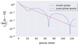
(a) $n\!=\!16$.

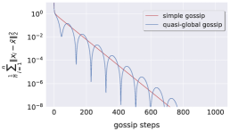
(b) $n\!=\!32$.

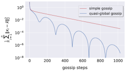
(c) $n\!=\!64$.

Figure 3: Understanding QG-DSGDm through the distributed average consensus problem on a fixed ring topology. QG-DSGDm without gradient update step (4) still presents faster convergence (to a relative high precision) than the standard gossip averaging. Appendix LABEL:appendix:more_on_consensus_averaging_problem illustrates the results on other communication topologies and topology scales.

3.3 Convergence Analysis

We provide a convergence analysis for our novel QG-DSGDm for non-convex functions. The proof details can be found in Appendix LABEL:appendix:convergence_rate_proofs.

Assumption 1.

We assume that the following hold:

• The function $f(\mathbf{x})$ we are minimizing is lower bounded from below by $f^{\star}$, and each node’s loss $f_{i}$ is smooth satisfying $\left\lVert\nabla f_{i}(\mathbf{y})\!-\!\nabla f_{i}(\mathbf{x})\right\rVert\leq L\left\lVert\mathbf{y}\!-\!\mathbf{x}\right\rVert$.

• The stochastic gradients within each node satisfy ${\mathbb{E}}\left[g_{i}(\mathbf{x})\right]\!=\!\nabla f_{i}(\mathbf{x})$ and ${\mathbb{E}}\left\lVert g_{i}(\mathbf{x})\!-\!\nabla f_{i}(\mathbf{x})\right\rVert^{2}\leq\sigma^{2}$. The variance across the workers is also bounded as $\frac{1}{n}\sum_{i=1}^{n}\left\lVert\nabla f_{i}(\mathbf{x})\!-\!\nabla f(\mathbf{x})\right\rVert^{2}\leq\zeta^{2}$.

• The mixing matrix is doubly stochastic: for the all ones vector $\mathbf{1}$, we have $\mathbf{W}\mathbf{1}\!=\!\mathbf{1}$ and $\mathbf{W}^{\top}\mathbf{1}\!=\!\mathbf{1}$.

• Define $\bar{\mathbf{Z}}\!=\!\mathbf{Z}\frac{1}{n}\mathbf{1}\mathbf{1}^{\top}$ for any matrix $\mathbf{Z}\in\mathbb{R}^{d\times n}$, then the mixing matrix satisfies ${\mathbb{E}}_{\mathbf{W}}\left\lVert\mathbf{Z}\mathbf{W}-\bar{\mathbf{Z}}\right\rVert_{F}^{2}\leq(1-\rho)\left\lVert\mathbf{Z}-\bar{\mathbf{Z}}\right\rVert_{F}^{2}$.

Theorem 3.1 (Convergence of QG-DSGDm for non-convex functions).

Given Assumption 1, the sequence of iterates generated by (3) for step size $\eta\!=\!\smash{\mathcal{O}\left(\sqrt{\frac{n}{\sigma^{2}T}}\right)}$ and momentum parameter $\frac{\beta}{1-\beta}\leq\frac{\rho}{21}$ satisfies $\frac{1}{T}\sum_{t=0}^{T-1}{\mathbb{E}}\left\lVert\nabla f(\bar{\mathbf{x}}^{t})\right\rVert^{2}\leq\epsilon$ in iterations

$$\textstyle T=\mathcal{O}\Big{(}\frac{L\sigma^{2}}{n\epsilon^{2}}+\frac{L\tilde{\zeta}}{\rho\epsilon^{3/2}}+\frac{L}{\epsilon}(\frac{1}{\rho}+\frac{1}{(1-\mu)(1-\beta)^{2}})\Big{)}\,,$$

where $\tilde{\zeta}^{2}:=\zeta^{2}+(1+\frac{1-\beta}{1-\mu})\sigma^{2}$.

Remark 3.2.

The asymptotic number of iterations required, $\mathcal{O}\bigl{(}\frac{\sigma^{2}}{n\epsilon^{2}}\bigr{)}$ shows perfect linear speedup in the number of workers $n$, independent of the communication topology. This upper bound matches the convergence bounds of DSGD (Lian et al., 2017) and centralized mini-batch SGD (Dekel et al., 2012), and is optimal (Arjevani et al., 2019). This significantly improves over previous analyses of distributed momentum methods which need $\frac{L\sigma^{2}}{n(1-\beta)\epsilon^{2}}$ iterations, slowing down for larger values of $\beta$ (Yu et al., 2019; Balu et al., 2020). The second drift term $\frac{1}{\rho\epsilon^{3/2}}$ arises due to the non-iid data distribution, and matches the tightest analysis of DSGD without momentum (Koloskova et al., 2020b). Finally, our theorem imposes some constraint on the momentum parameter $\beta$ (but not on $\mu$). In practice however, QG-DSGDm performs well even when this constraint is violated.

3.4 Connection with Other Methods

We bridge quasi-global momentum with two recent works below. The corresponding algorithm details are included in Appendix B.1 for clarity.

Connection with MimeLite.

MimeLite (Karimireddy et al., 2020a) was recently introduced for FL on heterogeneous data. It shares a similar ingredient as ours: a “global” movement direction $\mathbf{d}$ is used locally to alleviate the issue caused by heterogeneity. The difference falls into the way of forming $\mathbf{d}$ (c.f. line 8 in Algorithm 1): in MimeLite, $\mathbf{d}$ is the full batch gradients computed on the previously synchronized model, while the $\mathbf{d}$ in our QG-DSGDm is the difference on two consecutive synchronized models.
MimeLite only addresses the FL setting, which results in a computation and communication overhead (to form $\mathbf{d}$), and is non-trivial to extend to decentralized learning.

Connection with SlowMo.

SlowMo and its “noaverage” variant (Wang et al., 2020c) aim to improve generalization performance in the homogeneous data-center training scenario, while QG-DSGDm is targeting learning with data heterogeneity. In terms of update scheme, SlowMo variants update the slow momentum buffer through the model difference $\mathbf{d}$ of $\tau\!\gg\!1$ local update (and synchronization) steps, while QG-DSGDm only considers consecutive models (analogously $\tau\!=\!1$). Besides, in contrast to QG-DSGDm, the slow momentum buffer in SlowMo will never interact with the local update—setting $\tau$ to 1 in SlowMo variants cannot recover QG-DSGDm.
SlowMo variants are orthogonal to QG-DSGDm; combining these two algorithms may lead to a better generalization performance, and we leave it for future work.

4 Understanding QG-DSGDm

4.1 Faster Convergence in Average Consensus

We now consider the simpler averaging consensus problem (isolated from the learning part of QG-DSGDm): we simplify (3) by removing gradients and step-size:

$$\textstyle\begin{split}\textstyle\mathbf{X}^{(t+1)}&\textstyle=\mathbf{W}\left(\mathbf{X}^{(t)}-\beta\mathbf{M}^{(t-1)}\right)\\ \textstyle\mathbf{M}^{(t)}&\textstyle=\mu\mathbf{M}^{(t-1)}+(1-\mu)\left(\mathbf{X}^{(t)}-\mathbf{X}^{(t+1)}\right)\,,\end{split}$$ (4)

and compare it with gossip averaging $\mathbf{X}^{(t+1)}=\mathbf{W}\mathbf{X}^{(t)}$.

Figure 3 depicts the advantages of (4) over standard gossip averaging, where QG-DSGDm can quickly converge to a critical consensus distance (e.g. $10^{-2}$). It partially explains the performance gain of QG-DSGDm from the aspect of improved decentralized communication (which leads to better optimization)—decentralized training can converge as fast as its centralized counterpart once the consensus distance is lower than the critical one, as stated in (Kong et al., 2021).

4.2 QG-DSGDm (Single Worker Case) Recovers QHM

Considering the single worker case, QG-DSGDm can be further simplified to (derivations in Appendix LABEL:appendix:hd_sgd_with_single_worker_sgdm):

$$\textstyle\begin{split}\textstyle\hat{\mathbf{m}}^{(t)}&\textstyle=\hat{\beta}\hat{\mathbf{m}}^{(t-1)}+\mathbf{g}^{(t)}\\ \textstyle\mathbf{x}^{(t+1)}&\textstyle=\mathbf{x}^{(t)}-\eta\left((1-\frac{\mu}{\hat{\beta}})\hat{\mathbf{m}}^{(t)}+\frac{\mu}{\hat{\beta}}\mathbf{g}^{(t)}\right)\,,\end{split}$$

where $\hat{\beta}:=\mu+(1-\mu)\beta$. Thus, the single worker case of QG-DSGDm (i.e. QG-SGDm) recovers Quasi-Hyperbolic Momentum (QHM) (Ma & Yarats, 2019; Gitman et al., 2019). We illustrate its acceleration benefits as well as the performance gain in Figure LABEL:fig:understanding_optsgd_on_n1_complete and Figure LABEL:fig:understanding_optsgd_on_n1_and_wo_weight_decay of Appendix LABEL:appendix:understanding_single_worker. We elaborate in Appendix LABEL:appendix:connection_for_single_worker_case that SGDm is only a special case of QG-SGDm/QHM (by setting $\mu\!=\!0$). Besides, it is non-trivial to adapt (centralized) QHM to (decentralized) QG-DSGDm due to discrepant motivation.

Stabilized optimization trajectory.

We study the optimization trajectory of Rosenbrock function (Rosenbrock, 1960) $f(x,y)=(y-x^{2})^{2}+100(x-1)^{2}$ as in (Lucas et al., 2019) to better understand the performance gain of QG-SGDm (with zero stochastic noise). Figure LABEL:fig:understanding_on_new_2d_toy_example_complete illustrates the effects of stabilization in QG-SGDm (much less oscillation than SGDm).

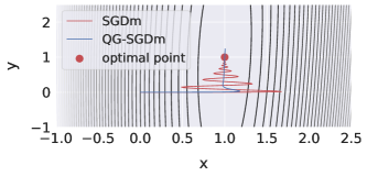
Figure 4: Understanding the optimization trajectory of QG-SGDm and SGDm (i.e. single worker case) via a 2D toy function $f(x,y)=(y-x^{2})^{2}+100(x-1)^{2}$. This function has a global minimum at $(x,y)=(1,1)$. SGDm and QG-SGDm use $\beta=0.9,\eta=0.001$, with initial point $(0,0)$. For additional trajectories with different initial points and/or $\beta$ values refer to Appendix LABEL:appendix:toy_problem_trajectory.

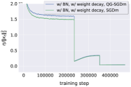
(a) ResNet-BN-20.

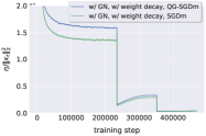
(b) ResNet-GN-20.

Figure 5: The effective step-size $\eta/\left\lVert\mathbf{x}_{t}\right\rVert_{2}^{2}$ of QG-SGDm and SGDm (single worker case) on CIFAR-10. For the weight norm curves refer to Figure LABEL:fig:n1_resnet20_cifar10_understanding_from_deep_learning_aspect_complete in Appendix LABEL:appendix:understanding_single_worker.

Larger effective step-size.

Recent works (Hoffer et al., 2018; Zhang et al., 2019) point out the larger effective step-size (i.e. $\eta/\left\lVert\mathbf{x}_{t}\right\rVert_{2}^{2}$) brought by weight decay provides the primary regularization effect for deep learning training. Figure 5 examines the effective step-size during the optimization procedure: QG-SGDm illustrates a larger effective step-size than SGDm, explaining the performance gain e.g. in Figure LABEL:fig:understanding_optsgd_on_n1_complete and Figure LABEL:fig:understanding_optsgd_on_n1_and_wo_weight_decay of Appendix LABEL:appendix:understanding_single_worker.

5 Experiments

5.1 Setup

Datasets and models.

We empirically study the decentralized training behavior on both CV and NLP benchmarks, on the architecture of ResNet (He et al., 2016), VGG (Simonyan & Zisserman, 2014) and DistilBERT (Sanh et al., 2019). $\bullet$ Image classification (CV) benchmark: we consider training CIFAR-10 (Krizhevsky & Hinton, 2009), ImageNet-32 (i.e. image resolution of $32$) (Chrabaszcz et al., 2017), and ImageNet (Deng et al., 2009) from scratch, with standard data augmentation and preprocessing scheme (He et al., 2016). We use VGG-11 (with width factor $1/2$ and without BN) and ResNet-20 for CIFAR-10, ResNet-20 with width factor $2$ (noted as ResNet-20-x2) for ImageNet-32, and ResNet-18 for ImageNet. The width factor indicates the proportional scaling of the network width corresponding to the original neural network. Weight initialization schemes follow (He et al., 2015; Goyal et al., 2017). $\bullet$ Text classification (NLP) benchmark: we perform fine-tuning on a $4$-class classification dataset (AG News (Zhang et al., 2015)). Unless mentioned otherwise, all our experiments are repeated over three random seeds. We report the averaged performance of local models on the full test dataset.

Table 1: The test top-1 accuracy of different decentralized optimization algorithms evaluated on different degrees of non-i.i.d. local CIFAR-10 data, for various neural architectures and network topologies. The results are averaged over three random seeds, with learning rate tuning for each setting. We also include the results of centralized baseline for reference purposes, following the decentralized experiment configuration, except that the centralized baseline uses randomly partitioned local training data (i.e. independent of $\alpha$).

Datasets	Neural Architectures	Methods	Ring ($n\!=\!16$)			Social Network ($n\!=\!32$)
			$\alpha=10$	$\alpha=1$	$\alpha=0.1$	$\alpha=10$	$\alpha=1$	$\alpha=0.1$
CIFAR-10	ResNet-BN-20	SGDm-N (centralized)	$92.95\pm 0.13$			$92.88\pm 0.07$
		DSGD	$90.94\pm 0.15$	$88.95\pm 0.59$	$54.66\pm 3.58$	$90.52\pm 0.24$	$89.22\pm 0.35$	$58.32\pm 3.27$
		DSGDm-N	$92.53\pm 0.27$	$89.13\pm 0.81$	$57.19\pm 2.65$	$92.20\pm 0.24$	$90.19\pm 0.54$	$63.00\pm 2.50$
		QG-DSGDm-N	$\textbf{92.65}\pm 0.17$	$\textbf{91.21}\pm 0.28$	$\textbf{58.16}\pm 3.32$	$\textbf{92.52}\pm 0.09$	$\textbf{91.20}\pm 0.16$	$\textbf{64.32}\pm 2.43$
	ResNet-GN-20	SGDm-N (centralized)	$88.06\pm 1.12$			$86.19\pm 1.08$
		DSGD	$86.86\pm 0.37$	$85.93\pm 0.14$	$73.14\pm 3.92$	$84.00\pm 0.67$	$82.98\pm 0.47$	$67.84\pm 3.94$
		DSGDm-N	$89.86\pm 0.15$	$88.30\pm 0.49$	$71.86\pm 2.22$	$88.54\pm 0.22$	$86.36\pm 0.55$	$72.02\pm 1.79$
		QG-DSGDm-N	$\textbf{90.18}\pm 0.44$	$\textbf{89.68}\pm 0.41$	$\textbf{82.78}\pm 2.05$	$\textbf{88.58}\pm 0.09$	$\textbf{88.19}\pm 0.30$	$\textbf{83.60}\pm 1.83$
	ResNet-EvoNorm-20	SGDm-N (centralized)	$92.18\pm 0.19$			$91.92\pm 0.33$
		DSGD	$89.90\pm 0.26$	$88.88\pm 0.26$	$74.55\pm 2.07$	$89.95\pm 0.23$	$88.41\pm 0.27$	$77.56\pm 1.65$
		DSGDm-N	$91.47\pm 0.23$	$89.98\pm 0.10$	$77.48\pm 2.67$	$91.17\pm 0.11$	$89.96\pm 0.35$	$80.59\pm 2.32$
		QG-DSGDm-N	$\textbf{91.90}\pm 0.17$	$\textbf{91.28}\pm 0.38$	$\textbf{82.20}\pm 1.27$	$\textbf{91.51}\pm 0.02$	$\textbf{91.00}\pm 0.24$	$\textbf{85.19}\pm 0.98$
	VGG-11 (w/o normalization layer)	SGDm-N (centralized)	$88.87\pm 0.29$			$87.38\pm 0.39$
		DSGDm-N	$88.68\pm 0.30$	$88.52\pm 0.24$	$77.45\pm 3.15$	$86.39\pm 0.06$	$85.85\pm 0.22$	$77.02\pm 2.66$
		QG-DSGDm-N	$\textbf{89.01}\pm 0.04$	$\textbf{89.00}\pm 0.22$	$\textbf{83.41}\pm 2.20$	$\textbf{86.87}\pm 0.60$	$\textbf{86.09}\pm 0.30$	$\textbf{84.86}\pm 0.58$

Heterogeneous distribution of client data.

We use the Dirichlet distribution to create disjoint non-i.i.d. client training data (Yurochkin et al., 2019; Hsu et al., 2019; He et al., 2020)—the created client data is fixed and never shuffled across clients during the training. The degree of non-i.i.d.-ness is controlled by the value of $\alpha$; the smaller $\alpha$ is, the more likely the clients hold examples from only one class. An illustration regarding how samples are distributed among $16$ clients on CIFAR-10 can be found in Figure 1; more visualizations on other datasets/scales are shown in Appendix A.2. Besides, Figure 7 in Appendix A.1 visualizes the Social Network topology.

Training schemes.

Following the SOTA deep learning training scheme, we use mini-batch SGD as the base optimizer for CV benchmark (He et al., 2016; Goyal et al., 2017), and similarly, Adam for NLP benchmark (Zhang et al., 2020; Mosbach et al., 2021). In Section 5.2, we adapt these base optimizers to different distributed variants.

For the CV benchmark, the models are trained for $300$ and $90$ epochs for CIFAR-10 and ImageNet(-32) respectively; the local mini-batch size are set to $32$ and $64$. All experiments use the SOTA learning rate scheme in distributed deep learning training (Goyal et al., 2017; He et al., 2019) with learning rate scaling and warm-up. The learning rate is always gradually warmed up from a relatively small value (i.e. $0.1$) for the first $5$ epochs. Besides, the learning rate will be divided by $10$ when the model has accessed specified fractions of the total number of training samples—$\{\frac{1}{2},\frac{3}{4}\}$ for CIFAR and $\{\frac{1}{3},\frac{2}{3},\frac{8}{9}\}$ for ImageNet.
For the NLP benchmark, we fine-tune the distilbert-base-uncased from HuggingFace (Wolf et al., 2019) with constant learning rate and mini-batch of size $32$ for $10$ epochs.

We fine-tune the learning rate for both CV and NLP tasks; we use constant weight decay (1e-4). The tuning procedure ensures that the best hyper-parameter lies in the middle of our search grids; otherwise we extend our search grid.
Regarding momentum related hyper-parameters, we follow the common practice in the community ($\beta\!=\!0.9$ and without dampening for Nesterov/HeavyBall momentum variants, and $\beta_{1}\!=\!0.9,\beta_{2}\!=\!0.99$ for Adam variants).

BN and its alternatives for distributed deep learning.

The existence of BN layer is challenging for the SOTA distributed training, especially for heterogeneous data setting. To better understand the impact of different normalization schemes in distributed deep learning, we investigate:

• Distributed BN implementation. Our default implementation follows (Goyal et al., 2017; Andreux et al., 2020) that computes the BN statistics independently for each client while only synchronizing the BN weights.

• Using other normalization layers: for instance on ResNet with BN layers (denoted by ResNet-BN-20), we can instead use ResNet-GN by replacing all BN with GN with group number of $2$, as suggested in (Hsieh et al., 2020). We also examine the recently proposed S0 variant of EvoNorm (Liu et al., 2020) (which does not use runtime mini-batches statistics), noted as ResNet-EvoNorm.

Table 2: Comparison with Gradient Tracking (GT) methods for training CIFAR-10. D${}^{2}$ and D${}^{2}_{+}$ do not include the momentum acceleration. We carefully tune the learning rate for each case, and results are averaged over three seeds where std is indicated.

	ResNet-EvoNorm-20 on Ring ($n\!=\!16$)						ResNet-EvoNorm-20 on Ring ($n\!=\!32$)
	DSGD (w/ GT)	DSGDm-N	DSGDm-N (w/ GT)	D${}^{2}$	D${}^{2}_{+}$	QG-DSGDm-N	DSGDm-N	DSGDm-N (w/ GT)	QG-DSGDm-N
$\alpha\!=\!1$	$87.36\pm 0.40$	$89.98\pm 0.10$	$90.38\pm 0.41$	$74.89$	$85.70\pm 0.29$	$\textbf{91.28}\pm 0.38$	$88.46\pm 0.29$	$89.44\pm 0.60$	$\textbf{90.27}\pm 0.27$
$\alpha\!=\!0.1$	$66.16\pm 1.05$	$77.48\pm 2.67$	$78.64\pm 1.84$	$49.80$	$69.18\pm 3.30$	$\textbf{82.20}\pm 1.27$	$78.17\pm 1.63$	$79.25\pm 2.17$	$\textbf{83.18}\pm 1.11$

5.2 Results

Comments on BN and its alternatives.

Table 1 and Table 3 examine the effects of BN and its alternatives on the training quality of decentralized deep learning on CIFAR-10 and ImageNet dataset. ResNet with EvoNorm replacement outperforms its GN counterpart on a spectrum of optimization algorithms, non-i.i.d. degrees, and network topologies, illustrating its efficacy to be a new alternative to BN in CNNs for distributed learning on heterogeneous data.

Superior performance of quasi-global momentum.

We evaluate QG-DSGDm-N and compare it with several DSGD variants in Table 1, for training different neural networks on CIFAR-10 in terms of different non-i.i.d. degrees on Ring ($n\!=\!16$) and Social Network ($n\!=\!32$). QG-DSGDm-N accelerates the training by stabilizing the oscillating optimization trajectory caused by heterogeneity and leads to a significant performance gain over all other strong competitors on all levels of data heterogeneity. The benefits of our method are further pronounced when considering a higher degree of non-i.i.d.-ness. These observations are consistent with the results on the challenging ImageNet(-32) dataset in Table 3 (and the learning curves in Figure LABEL:fig:learning_curves_cv_tasks in Appendix LABEL:appendix:learning_curves_cv_task).

Table 3: Test top-1 accuracy of different decentralized optimization algorithms evaluated on different degrees of non-i.i.d. local ImageNet data. The results are over three random seeds. We perform sufficient learning rate tuning on ImageNet-32 for each setup while we use the same one for ImageNet due to the computational feasibility. “$\star$” indicates non-convergence.

Datasets	Neural Architectures	Methods	Ring ($n\!=\!16$)
			$\alpha=1$	$\alpha=0.1$
ImageNet-32 (resolution 32)	ResNet-20-x2 (EvoNorm)	SGDm-N (centralized)	$44.43\pm 0.20$
		DSGDm-N	$30.35\pm 0.05$	$16.71\pm 0.17$
		QG-DSGDm-N	$\textbf{31.24}\pm 0.27$	$\textbf{19.53}\pm 0.91$
	ResNet-20-x2 (GN)	SGDm-N (centralized)	$37.89\pm 0.67$
		DSGDm-N	$34.16\pm 1.37$	$\star$
		QG-DSGDm-N	$\textbf{38.57}\pm 0.45$	$\textbf{21.42}\pm 0.81$
ImageNet	ResNet-18 (EvoNorm)	SGDm-N (centralized)	$69.55\pm 0.25$
		DSGDm-N	$68.77\pm 0.05$	$53.15\pm 0.14$
		QG-DSGDm-N	$\textbf{69.20}\pm 0.08$	$\textbf{56.50}\pm 0.01$
	ResNet-18 (GN)	SGDm-N (centralized)	$62.59\pm 0.01$
		DSGDm-N	$60.76\pm 0.48$	$39.57\pm 1.22$
		QG-DSGDm-N	$\textbf{64.92}\pm 0.27$	$\textbf{47.86}\pm 1.05$

Table 4: Test top-1 accuracy of different decentralized SGD algorithms evaluated on different degrees of non-i.i.d.-ness and communication topologies, for training ResNet-EvoNorm-18 on ImageNet. The results are over three random seeds. We use the same learning rate for different experiments due to the computational feasibility. Centralized SGDm-N reaches $69.55\pm 0.25$.

Communication Topology	Methods	Test Top-1 Accuracy
		$\alpha=1$	$\alpha=0.1$
Ring ($n\!=\!16$)	DSGDm-N	$68.77\pm 0.05$	$53.15\pm 0.14$
	QG-DSGDm-N	$\textbf{69.20}\pm 0.08$	$\textbf{56.50}\pm 0.01$
1-peer directed exponential graph ($n\!=\!16$) (Assran et al., 2019)	DSGDm-N	$69.00\pm 0.11$	$58.52\pm 0.27$
	QG-DSGDm-N	$\textbf{69.34}\pm 0.17$	$\textbf{61.44}\pm 0.20$

Decentralized Adam.

We further extend the idea of quasi-global momentum to the Adam optimizer for decentralized learning, noted as QG-DAdam (the algorithm details are deferred to Algorithm 2 in Appendix B.1). We validate the effectiveness of QG-DAdam over D(decentralized)Adam in Table 6, on fine-tuning DistilBERT on AG News and training ResNet-EvoNorm-20 on CIFAR-10 from scratch: QG-DAdam is still preferable over DAdam. We leave a better adaptation and theoretical proof for future work.

Generalizing quasi-global momentum to time-varying topologies.

The benefits of quasi-global momentum are not limited to the fixed and undirected communication topologies, e.g. Ring and Social network in Table 1—it also generalizes to other topologies, like the time-varying directed topology (Assran et al., 2019), as shown in Table 4 for training ResNet-EvoNorm-18 on ImageNet. These results are aligned with the findings on the influence of the consensus distance on the generalization performance of decentralized deep learning (Kong et al., 2021), supporting the fact that quasi-global momentum can be served as a simple plugin to further improve the performance of decentralized deep learning.

Table 5: An extensive investigation for a wide spectrum of DSGD variants, for training ResNet-EvoNorm-20 on CIFAR-10. The results are averaged over three seeds, each with learning rate tuning. We use “communication topology” to synchronize the model parameters, while some methods involve “extra communication”, with specified objective to be communicated on the given network topology.

Methods	Communication Topology	Extra Communication	Momentum Type	Test Top-1 Accuracy ($n\!=\!16$)
				$\alpha=1$	$\alpha=0.1$
SGDm-N	complete	-	global	$92.18\pm 0.19$
DSGDm-N	complete	-	local	$91.47\pm 0.10$	$71.24\pm 3.08$
DSGDm-N	ring	momentum buffer (complete)	local	$90.96\pm 0.33$	$81.22\pm 1.78$
SlowMo	ring	model parameters (complete)	local & global	$91.06\pm 0.26$	$79.20\pm 1.16$
DSGD	ring	-	-	$88.88\pm 0.26$	$74.55\pm 2.07$
DSGDm	ring	-	local	$89.67\pm 0.33$	$77.66\pm 0.95$
DSGDm-N	ring	-	local	$89.98\pm 0.10$	$77.48\pm 2.67$
DSGDm	ring	momentum buffer (ring)	local	$90.42\pm 0.32$	$78.69\pm 2.39$
DSGDm-N	ring	momentum buffer (ring)	local	$90.48\pm 0.67$	$79.83\pm 2.29$
DSGDm-N	ring	local gradients (ring)	local	$90.10\pm 0.61$	$78.58\pm 4.12$
DMSGD	ring	-	local	$90.06\pm 0.04$	$79.89\pm 0.97$
QG-DSGDm	ring	-	local	$91.22\pm 0.41$	$\textbf{82.24}\pm 1.05$
QG-DSGDm-N	ring	-	local	$\textbf{91.28}\pm 0.38$	$82.20\pm 1.27$

Table 6: Test accuracy of different decentralized optimization algorithms (with Adam), evaluated on different degrees of non-i.i.d. local data. The results are over three random seeds, with tuned learning rate.

Models & Datasets	Methods	$\alpha=0.1$
Fine-tuning DistilBERT-base (AG News)	DAdam	$87.29\pm 0.60$
	QG-DAdam	$\textbf{88.33}\pm 0.67$
Training ResNet-EvoNorm-20 from scratch (CIFAR-10)	DAdam	$65.52\pm 3.32$
	QG-DAdam	$\textbf{66.86}\pm 2.81$

Comparison with D${}^{2}$ and Gradient Tracking (GT).

As shown in Table 2, D${}^{2}$ (Tang et al., 2018b) and GT methods (Pu & Nedić, 2020; Pan et al., 2020; Lu et al., 2019) cannot achieve comparable test performance on the standard deep learning benchmark, while QG-DSGDm-N outperforms them significantly. Additional detailed comparisons are deferred to Appendix LABEL:appendix:comparison_with_gradient_tracking.
It is non-trivial to integrate D${}^{2}$ with momentum. Besides, D${}^{2}$ requires constant learning rate, which does not fit the SOTA learning rate schedules (e.g. stage-wise) in deep learning. We include an improved D${}^{2}$ variant (denoted as D${}^{2}_{+}$) to address this learning rate decay issue in D${}^{2}$, but the performance of D${}^{2}_{+}$ still remains far behind our scheme.

Ablation study.

Table 5 empirically investigates a wide range of different DSGD variants, in terms of the generalization performance on different degrees of data heterogeneity. We can witness that (1) DSGD variants with quasi-global momentum always significantly surpass all other methods (excluding the centralized upper bound), without introducing extra communication cost; (2) local momentum accelerates the decentralized optimization (c.f. the results of DSGD v.s. DSGDm and DSGDm-N), while our quasi-global momentum further improves the performance gain; (3) synchronizing local momentum buffer or local gradients only marginally improves the generalization performance, but the gains fall behind our quasi-global momentum (as we accelerate the consensus and stabilize trajectories, as illustrated in Section 4); (4) the parallel work DMSGD (Balu et al., 2020) does show some improvements, but its performance gain is much less significant than ours. Table LABEL:fig:tuning_momentum_factors in the Appendix LABEL:appendix:tuning_lr_and_momentum_for_sgdmN further shows that tuning momentum factor for DSGDm-N cannot alleviate the training difficulty caused by data heterogeneity.

Besides, Figure 6 showcases the generality of quasi-global momentum for achieving remarkable performance gain on different topology scales and non-i.i.d. degrees.

(a) $\alpha\!=\!1$.

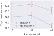
(b) $\alpha\!=\!0.1$.

Figure 6: Test top-1 accuracy of different decentralized algorithms evaluated on different topology scales and non-i.i.d. degrees, for training ResNet-EvoNorm-20 on CIFAR-10. The results are over three random seeds, each with sufficient learning rate tuning. Colors blue and red indicate DSGDm-N and QG-DSGDm-N respectively. Numerical results refer to Table LABEL:tab:cv_different_ring_scale_results in Appendix LABEL:appendix:cv_different_ring_scale_results.

Conclusion

We demonstrated that heterogeneity has an out sized impact on the performance of deep learning models, leading to unstable convergence and poor performance. We proposed a novel momentum-based algorithm to stabilize the training and established its efficacy through thorough empirical evaluations. Our method, especially for mildly heterogeneous settings, leads to a 10–20% increase in accuracy. However, a gap still remains between the centralized training. Closing this gap, we believe, is critical for wider adoption of decentralized learning.

Appendix A Detailed Experimental Setup

A.1 Visualization for Communication Topologies

Figure 7 visualizes the Social Network topology we evaluated in the main paper.

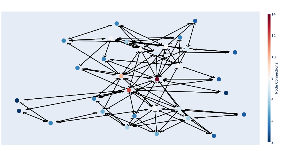
Figure 7: The visualization of the examined social topology (generated from “networkx.generators.social.davis_southern_women_graph”).

A.2 Visualization of Non-IID Local Data

The synthetic formulation of non-i.i.d. client data.

We re-iterate the partition scheme introduced and stated in (Yurochkin et al., 2019; Hsu et al., 2019) for completeness reasons.

Assume every client training example is drawn independently with class labels following a categorical distribution over $M$ classes parameterized by a vector $\mathbf{q}$ ($q_{i}\geq 0,i\in[1,M]$ and $\left\lVert\mathbf{q}\right\rVert_{1}=1$). To synthesize client non-i.i.d. local data distributions, we draw $\alpha\sim\text{Dir}(\alpha\mathbf{p})$ from a Dirichlet distribution, where $\mathbf{p}$ characterizes a prior class distribution over $M$ classes, and $\alpha>0$ is a concentration parameter controlling the identicalness among clients. With $\alpha\rightarrow\infty$, all clients have identical distributions to the prior; with $\alpha\rightarrow 0$, each client holds examples from only one random class.

To better understand the local data distribution for the datasets we considered in the experiments, in Figure 8 we visualize the partition results of CIFAR-10 and ImageNet(-32) for various degrees of non-i.i.d.-ness and network scales; in Figure 9, we visualize the partitioned local data on $16$ clients with $\alpha\!=\!\{10,1,0.1\}$ for AG News and SST-2.

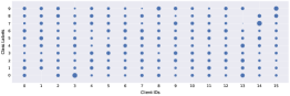
(a) CIFAR-10, $n\!=\!16$, $\alpha=10$.

(b) CIFAR-10, $n\!=\!16$, $\alpha=1$.

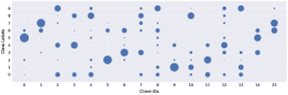
(c) CIFAR-10, $n\!=\!16$, $\alpha=0.1$.

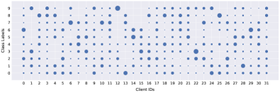
(d) CIFAR-10, $n\!=\!32$, $\alpha=1$.

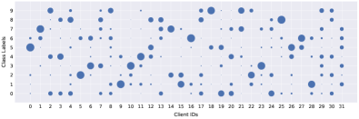
(e) CIFAR-10, $n\!=\!32$, $\alpha=0.1$.

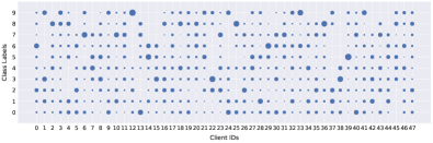
(f) CIFAR-10, $n\!=\!48$, $\alpha=1$.

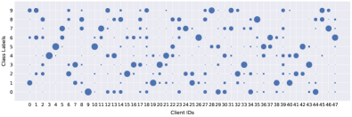
(g) CIFAR-10, $n\!=\!48$, $\alpha=0.1$.

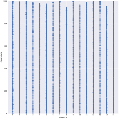
(h) ImageNet, $n\!=\!16$, $\alpha=1$.

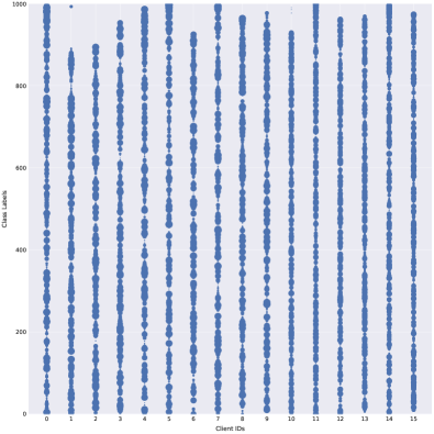
(i) ImageNet, $n\!=\!16$, $\alpha=0.1$.

Figure 8: Illustration of # of samples per class allocated to each client (indicated by dot sizes), for different Dirichlet distribution $\alpha$ values on CV datasets.

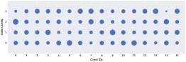
(a) AG News, $n\!=\!16$, $\alpha=10$.

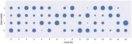
(b) AG News, $n\!=\!16$, $\alpha=1$.

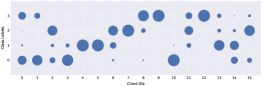
(c) AG News, $n\!=\!16$, $\alpha=0.1$.

Figure 9: Illustration of # of samples per class allocated to each client (indicated by dot sizes), for different Dirichlet distribution $\alpha$ values on NLP datasets.

Appendix B Detailed Algorithm Description and Connections

B.1 Detailed Algorithm Description

The variant of Adam with the idea of quasi-global momentum is detailed in Algorithm 2.

$t\in\{1,\ldots,T\}$sample $\xi_{i}^{(t)}$and compute $\mathbf{g}_{i}^{(t)}=\nabla F_{i}(\mathbf{x}_{i}^{(t)},\xi_{i}^{(t)})$$\mathbf{m}_{i}^{(t)}=\beta_{1}\hat{\mathbf{m}}_{i}^{(t-1)}+(1-\beta_{1})\hat{\mathbf{g}}_{i}^{(t)}$$\mathbf{v}_{i}^{(t)}=\beta_{2}\hat{\mathbf{v}}_{i}^{(t-1)}+(1-\beta_{2})\hat{\mathbf{g}}_{i}^{(t)}\odot\hat{\mathbf{g}}_{i}^{(t)}$$\mathbf{x}_{i}^{(t+\frac{1}{2})}=\mathbf{x}_{i}^{(t)}-\eta\frac{\mathbf{m}_{i}^{(t)}}{\sqrt{\mathbf{v}_{i}^{(t)}}+\epsilon}$$\mathbf{x}_{i}^{(t+1)}=\sum_{j\in\mathcal{N}_{i}^{(t)}}w_{ij}\mathbf{x}_{j}^{(t+\frac{1}{2})}$$\mathbf{d}_{i}^{(t)}=\mathbf{x}_{i}^{(t)}-\mathbf{x}_{i}^{(t+1)}$$\hat{\mathbf{d}}_{i}^{(t)}=\frac{\mathbf{d}_{i}^{(t)}}{\left\lVert\mathbf{d}_{i}^{(t)}\right\rVert_{2}}$$\hat{\mathbf{m}}_{i}^{(t)}=\beta_{1}\hat{\mathbf{m}}_{i}^{(t-1)}+(1-\beta_{1})\hat{\mathbf{d}}_{i}^{(t)}$$\hat{\mathbf{v}}_{i}^{(t)}=\beta_{2}\hat{\mathbf{v}}_{i}^{(t-1)}+(1-\beta_{2})\hat{\mathbf{d}}_{i}^{(t)}\odot\hat{\mathbf{d}}_{i}^{(t)}$$\mathbf{x}_{i}^{(T)}$

Algorithm 2 QG-DAdam. $\hat{\mathbf{m}}_{i}^{(0)},\hat{\mathbf{v}}_{i}^{(0)}$ are initialized as $\mathbf{0}$ for all workers.

worker-$i$$t\in\{1,\ldots,T\}$sample $\xi_{i}^{(t)}$and compute $\mathbf{g}_{i}^{(t)}=\nabla F_{i}(\mathbf{x}_{i}^{(t)},\xi_{i}^{(t)})$$\mathbf{m}_{i}^{(t)}=\beta\hat{\mathbf{m}}_{i}^{(t-1)}+\mathbf{g}_{i}^{(t)}$$\mathbf{x}_{i}^{(t+\frac{1}{2})}=\mathbf{x}_{i}^{(t)}-\eta\mathbf{m}_{i}^{(t)}$$\mathbf{x}_{i}^{(t+1)}=\sum_{j\in\mathcal{N}_{i}^{(t)}}w_{ij}\mathbf{x}_{j}^{(t+\frac{1}{2})}$$\text{mod}(t,\tau)\neq 0$$\hat{\mathbf{m}}_{i}^{(t)}=\hat{\mathbf{m}}_{i}^{(t-1)}$$\mathbf{d}_{i}^{(t)}=\frac{\mathbf{x}_{i}^{(t)}-\mathbf{x}_{i}^{(t+1)}}{\eta}$$\hat{\mathbf{m}}_{i}^{(t)}=\mu\hat{\mathbf{m}}_{i}^{(t-1)}+(1-\mu)\mathbf{d}_{i}^{(t)}$$\mathbf{x}_{i}^{(T)}$

Algorithm 3 Multiple-step variant of QG-DSGDm. $\mathbf{m}_{i}^{(0)}=\hat{\mathbf{m}}_{i}^{(0)}:=\mathbf{0}$. $\tau$ is the number of local steps.

Algorithm LABEL:alg:mimelite depicts the general procedure of MimeLite in (Karimireddy et al., 2020a). For SGDm, the update step $\mathcal{U}$ and the tracking step $\mathcal{V}$ follow

$$\begin{split}\mathcal{U}\left(\nabla F_{i}(\mathbf{y}_{i},\xi),\mathbf{s}\right)&:=(1-\beta)\nabla F_{i}(\mathbf{y}_{i},\xi)+\beta\mathbf{s}\\ \mathcal{V}\left(\frac{1}{\left\lvert\mathcal{S}\right\rvert}\sum_{i\in\mathcal{S}}\nabla f_{i}(\mathbf{x}),\mathbf{s}\right)&:=(1-\beta)\frac{1}{\left\lvert\mathcal{S}\right\rvert}\sum_{i\in\mathcal{S}}\nabla f_{i}(\mathbf{x})+\beta\mathbf{s}\,.\end{split}$$

each round $t\in[T]$sample subset $\mathcal{S}$of clients communicate $(\mathbf{x},\mathbf{s})$to all clients $i\in\mathcal{S}$client $i\in\mathcal{S}$in parallel initialize local model $\mathbf{y}_{i}\leftarrow\mathbf{x}$client $i\in\mathcal{S}$in parallel $k\in[\tau]$sample mini-batch $\xi$from local data $\mathbf{y}_{i}\leftarrow\mathbf{y}_{i}-\eta\mathcal{U}\left(\nabla F_{i}(\mathbf{y}_{i},\xi),\mathbf{s}\right)$compute full local-batch gradient $\nabla f_{i}(\mathbf{x})$communicate $(\mathbf{y}_{i},\nabla f_{i}(\mathbf{x}))$

References

- Andreux et al. (2020) Andreux, M., du Terrail, J. O., Beguier, C., and Tramel, E. W. Siloed federated learning for multi-centric histopathology datasets. In Domain Adaptation and Representation Transfer, and Distributed and Collaborative Learning, pp. 129–139. Springer, 2020.
- Arjevani et al. (2019) Arjevani, Y., Carmon, Y., Duchi, J. C., Foster, D. J., Srebro, N., and Woodworth, B. Lower bounds for non-convex stochastic optimization. arXiv preprint arXiv:1912.02365, 2019.
- Assran et al. (2019) Assran, M., Loizou, N., Ballas, N., and Rabbat, M. Stochastic gradient push for distributed deep learning. In International Conference on Machine Learning, pp. 344–353. PMLR, 2019.
- Balu et al. (2020) Balu, A., Jiang, Z., Tan, S. Y., Hedge, C., Lee, Y. M., and Sarkar, S. Decentralized deep learning using momentum-accelerated consensus. arXiv preprint arXiv:2010.11166, 2020.
- Bottou et al. (2016) Bottou, L., Curtis, F. E., and Nocedal, J. Optimization methods for large-scale machine learning. arXiv preprint arXiv:1606.04838, 2016.
- Boyd et al. (2006) Boyd, S., Ghosh, A., Prabhakar, B., and Shah, D. Randomized gossip algorithms. IEEE Transactions on Information Theory, 52(6):2508–2530, 2006.
- Chrabaszcz et al. (2017) Chrabaszcz, P., Loshchilov, I., and Hutter, F. A downsampled variant of ImageNet as an alternative to the CIFAR datasets. arXiv preprint arXiv:1707.08819, 2017.
- Das et al. (2020) Das, R., Acharya, A., Hashemi, A., Sanghavi, S., Dhillon, I. S., and Topcu, U. Faster non-convex federated learning via global and local momentum. arXiv preprint arXiv:2012.04061, 2020.
- Defazio & Bottou (2019) Defazio, A. and Bottou, L. On the ineffectiveness of variance reduced optimization for deep learning. In Advances in Neural Information Processing Systems, 2019.
- Dekel et al. (2012) Dekel, O., Gilad-Bachrach, R., Shamir, O., and Xiao, L. Optimal distributed online prediction using mini-batches. The Journal of Machine Learning Research, 13:165–202, 2012.
- Deng et al. (2009) Deng, J., Dong, W., Socher, R., Li, L.-J., Li, K., and Fei-Fei, L. ImageNet: A Large-Scale Hierarchical Image Database. In Proceedings of the IEEE/CVF Conference on Computer Vision and Pattern Recognition (CVPR), 2009.
- Diao et al. (2021) Diao, E., Ding, J., and Tarokh, V. HeteroFL: Computation and communication efficient federated learning for heterogeneous clients. In International Conference on Learning Representations, 2021. URL https://openreview.net/forum?id=TNkPBBYFkXg.
- Gitman et al. (2019) Gitman, I., Lang, H., Zhang, P., and Xiao, L. Understanding the role of momentum in stochastic gradient methods. In Advances in Neural Information Processing Systems, pp. 9633–9643, 2019.
- Goyal et al. (2017) Goyal, P., Dollár, P., Girshick, R., Noordhuis, P., Wesolowski, L., Kyrola, A., Tulloch, A., Jia, Y., and He, K. Accurate, large minibatch SGD: Training ImageNet in 1 hour. arXiv preprint arXiv:1706.02677, 2017.
- Haddadpour et al. (2021) Haddadpour, F., Kamani, M. M., Mokhtari, A., and Mahdavi, M. Federated learning with compression: Unified analysis and sharp guarantees. In International Conference on Artificial Intelligence and Statistics, pp. 2350–2358. PMLR, 2021.
- He et al. (2020) He, C., Li, S., So, J., Zhang, M., Wang, H., Wang, X., Vepakomma, P., Singh, A., Qiu, H., Shen, L., et al. Fedml: A research library and benchmark for federated machine learning. arXiv preprint arXiv:2007.13518, 2020.
- He et al. (2015) He, K., Zhang, X., Ren, S., and Sun, J. Delving deep into rectifiers: Surpassing human-level performance on imagenet classification. In Proceedings of the IEEE international conference on computer vision, pp. 1026–1034, 2015.
- He et al. (2016) He, K., Zhang, X., Ren, S., and Sun, J. Deep residual learning for image recognition. In Proceedings of the IEEE Conference on Computer Vision and Pattern Recognition, pp. 770–778, 2016.
- He et al. (2019) He, T., Zhang, Z., Zhang, H., Zhang, Z., Xie, J., and Li, M. Bag of tricks for image classification with convolutional neural networks. In Proceedings of the IEEE/CVF Conference on Computer Vision and Pattern Recognition, pp. 558–567, 2019.
- Hendrikx et al. (2019) Hendrikx, H., Bach, F., and Massoulié, L. Accelerated decentralized optimization with local updates for smooth and strongly convex objectives. In International Conference on Artificial Intelligence and Statistics, pp. 897–906. PMLR, 2019.
- Hoffer et al. (2018) Hoffer, E., Banner, R., Golan, I., and Soudry, D. Norm matters: efficient and accurate normalization schemes in deep networks. In Advances in Neural Information Processing Systems, pp. 2160–2170, 2018.
- Hsieh et al. (2020) Hsieh, K., Phanishayee, A., Mutlu, O., and Gibbons, P. The non-iid data quagmire of decentralized machine learning. In International Conference on Machine Learning, pp. 4387–4398. PMLR, 2020.
- Hsu et al. (2019) Hsu, T.-M. H., Qi, H., and Brown, M. Measuring the effects of non-identical data distribution for federated visual classification. arXiv preprint arXiv:1909.06335, 2019.
- Huang et al. (2016) Huang, G., Liu, Z., Weinberger, K. Q., and van der Maaten, L. Densely connected convolutional networks. arXiv preprint arXiv:1608.06993, 2016.
- Ioffe & Szegedy (2015) Ioffe, S. and Szegedy, C. Batch normalization: Accelerating deep network training by reducing internal covariate shift. arXiv preprint arXiv:1502.03167, 2015.
- Kairouz et al. (2019) Kairouz, P., McMahan, H. B., Avent, B., Bellet, A., Bennis, M., Bhagoji, A. N., Bonawitz, K., Charles, Z., Cormode, G., Cummings, R., et al. Advances and open problems in federated learning. arXiv preprint arXiv:1912.04977, 2019.
- Karimireddy et al. (2020a) Karimireddy, S. P., Jaggi, M., Kale, S., Mohri, M., Reddi, S. J., Stich, S. U., and Suresh, A. T. Mime: Mimicking centralized stochastic algorithms in federated learning. arXiv preprint arXiv:2008.03606, 2020a.
- Karimireddy et al. (2020b) Karimireddy, S. P., Kale, S., Mohri, M., Reddi, S. J., Stich, S. U., and Suresh, A. T. Scaffold: Stochastic controlled averaging for on-device federated learning. In International Conference on Machine Learning. PMLR, 2020b.
- Kempe et al. (2003) Kempe, D., Dobra, A., and Gehrke, J. Gossip-based computation of aggregate information. In 44th Annual IEEE Symposium on Foundations of Computer Science, 2003. Proceedings., pp. 482–491. IEEE, 2003.
- Koloskova et al. (2019) Koloskova, A., Stich, S. U., and Jaggi, M. Decentralized stochastic optimization and gossip algorithms with compressed communication. In International Conference on Machine Learning, volume 97, pp. 3479–3487. PMLR, 2019.
- Koloskova et al. (2020a) Koloskova, A., Lin, T., Stich, S. U., and Jaggi, M. Decentralized deep learning with arbitrary communication compression. In International Conference on Learning Representations, 2020a. URL https://openreview.net/forum?id=SkgGCkrKvH.
- Koloskova et al. (2020b) Koloskova, A., Loizou, N., Boreiri, S., Jaggi, M., and Stich, S. U. A unified theory of decentralized SGD with changing topology and local updates. In International Conference on Machine Learning. PMLR, 2020b.
- Konecnỳ et al. (2016) Konecnỳ, J., McMahan, H. B., Yu, F. X., Richtarik, P., Suresh, A. T., and Bacon, D. Federated learning: Strategies for improving communication efficiency. arXiv preprint arXiv:1610.05492, 2016.
- Kong et al. (2021) Kong, L., Lin, T., Koloskova, A., Jaggi, M., and Stich, S. U. Consensus control for decentralized deep learning. In International Conference on Machine Learning. PMLR, 2021.
- Krizhevsky & Hinton (2009) Krizhevsky, A. and Hinton, G. Learning multiple layers of features from tiny images. 2009.
- Lee et al. (2015) Lee, J. D., Lin, Q., Ma, T., and Yang, T. Distributed stochastic variance reduced gradient methods and a lower bound for communication complexity. arXiv preprint arXiv:1507.07595, 2015.
- Li et al. (2021) Li, X., Jiang, M., Zhang, X., Kamp, M., and Dou, Q. FedBN: Federated learning on non-IID features via local batch normalization. In International Conference on Learning Representations, 2021. URL https://openreview.net/forum?id=6YEQUn0QICG.
- Lian et al. (2017) Lian, X., Zhang, C., Zhang, H., Hsieh, C.-J., Zhang, W., and Liu, J. Can decentralized algorithms outperform centralized algorithms? a case study for decentralized parallel stochastic gradient descent. In Advances in Neural Information Processing Systems, pp. 5336–5346, 2017.
- Lian et al. (2018) Lian, X., Zhang, W., Zhang, C., and Liu, J. Asynchronous decentralized parallel stochastic gradient descent. In International Conference on Machine Learning, pp. 3043–3052. PMLR, 2018.
- Lin et al. (2020a) Lin, T., Kong, L., Stich, S., and Jaggi, M. Extrapolation for large-batch training in deep learning. In International Conference on Machine Learning, pp. 6094–6104. PMLR, 2020a.
- Lin et al. (2020b) Lin, T., Kong, L., Stich, S. U., and Jaggi, M. Ensemble distillation for robust model fusion in federated learning. In Advances in Neural Information Processing Systems, 2020b.
- Lin et al. (2020c) Lin, T., Stich, S. U., Patel, K. K., and Jaggi, M. Don’t use large mini-batches, use local SGD. In International Conference on Learning Representations, 2020c. URL https://openreview.net/forum?id=B1eyO1BFPr.
- Liu et al. (2020) Liu, H., Brock, A., Simonyan, K., and Le, Q. V. Evolving normalization-activation layers. arXiv preprint arXiv:2004.02967, 2020.
- Lu et al. (2019) Lu, S., Zhang, X., Sun, H., and Hong, M. GNSD: A gradient-tracking based nonconvex stochastic algorithm for decentralized optimization. In 2019 IEEE Data Science Workshop (DSW), pp. 315–321. IEEE, 2019.
- Lu & De Sa (2020) Lu, Y. and De Sa, C. Moniqua: Modulo quantized communication in decentralized sgd. In International Conference on Machine Learning, 2020.
- Lucas et al. (2019) Lucas, J., Sun, S., Zemel, R., and Grosse, R. Aggregated momentum: Stability through passive damping. In International Conference on Learning Representations, 2019. URL https://openreview.net/forum?id=Syxt5oC5YQ.
- Luo et al. (2019) Luo, P., Wang, X., Shao, W., and Peng, Z. Towards understanding regularization in batch normalization. In International Conference on Learning Representations, 2019. URL https://openreview.net/forum?id=HJlLKjR9FQ.
- Ma & Yarats (2019) Ma, J. and Yarats, D. Quasi-hyperbolic momentum and Adam for deep learning. In International Conference on Learning Representations, 2019. URL https://openreview.net/forum?id=S1fUpoR5FQ.
- McMahan et al. (2017) McMahan, B., Moore, E., Ramage, D., Hampson, S., and y Arcas, B. A. Communication-efficient learning of deep networks from decentralized data. In Artificial Intelligence and Statistics, pp. 1273–1282, 2017.
- Mosbach et al. (2021) Mosbach, M., Andriushchenko, M., and Klakow, D. On the stability of fine-tuning {bert}: Misconceptions, explanations, and strong baselines. In International Conference on Learning Representations, 2021. URL https://openreview.net/forum?id=nzpLWnVAyah.
- Nadiradze et al. (2020) Nadiradze, G., Sabour, A., Alistarh, D., Sharma, A., Markov, I., and Aksenov, V. SwarmSGD: Scalable decentralized SGD with local updates. arXiv preprint arXiv:1910.12308, 2020.
- Nedić et al. (2018) Nedić, A., Olshevsky, A., and Rabbat, M. G. Network topology and communication-computation tradeoffs in decentralized optimization. Proceedings of the IEEE, 106(5):953–976, 2018.
- Neglia et al. (2020) Neglia, G., Xu, C., Towsley, D., and Calbi, G. Decentralized gradient methods: does topology matter? In International Conference on Artificial Intelligence and Statistics, 2020.
- Pan et al. (2020) Pan, T., Liu, J., and Wang, J. D-SPIDER-SFO: A decentralized optimization algorithm with faster convergence rate for nonconvex problems. In Proceedings of the AAAI Conference on Artificial Intelligence, volume 34, pp. 1619–1626, 2020.
- Pu & Nedić (2020) Pu, S. and Nedić, A. Distributed stochastic gradient tracking methods. Mathematical Programming, pp. 1–49, 2020.
- Rosenbrock (1960) Rosenbrock, H. An automatic method for finding the greatest or least value of a function. The Computer Journal, 3(3):175–184, 1960.
- Sanh et al. (2019) Sanh, V., Debut, L., Chaumond, J., and Wolf, T. DistilBERT, a distilled version of BERT: smaller, faster, cheaper and lighter. arXiv preprint arXiv:1910.01108, 2019.
- Santurkar et al. (2018) Santurkar, S., Tsipras, D., Ilyas, A., and Madry, A. How does batch normalization help optimization? In Advances in Neural Information Processing Systems, pp. 2483–2493, 2018.
- Scaman et al. (2017) Scaman, K., Bach, F., Bubeck, S., Lee, Y. T., and Massoulié, L. Optimal algorithms for smooth and strongly convex distributed optimization in networks. In International Conference on Machine Learning. PMLR, 2017.
- Scaman et al. (2018) Scaman, K., Bach, F., Bubeck, S., Massoulié, L., and Lee, Y. T. Optimal algorithms for non-smooth distributed optimization in networks. In Advances in Neural Information Processing Systems, pp. 2740–2749, 2018.
- Shi et al. (2015) Shi, W., Ling, Q., Wu, G., and Yin, W. Extra: An exact first-order algorithm for decentralized consensus optimization. SIAM Journal on Optimization, 25(2):944–966, 2015.
- Simonyan & Zisserman (2014) Simonyan, K. and Zisserman, A. Very deep convolutional networks for large-scale image recognition. arXiv preprint arXiv:1409.1556, 2014.
- Singh et al. (2020) Singh, N., Data, D., George, J., and Diggavi, S. SQuARM-SGD: Communication-efficient momentum SGD for decentralized optimization. arXiv preprint arXiv:2005.07041, 2020.
- Sutskever et al. (2013) Sutskever, I., Martens, J., Dahl, G., and Hinton, G. On the importance of initialization and momentum in deep learning. In International Conference on Machine Learning, pp. 1139–1147. PMLR, 2013.
- Taheri et al. (2020) Taheri, H., Mokhtari, A., Hassani, H., and Pedarsani, R. Quantized decentralized stochastic learning over directed graphs. In International Conference on Machine Learning, pp. 9324–9333. PMLR, 2020.
- Tan & Le (2019) Tan, M. and Le, Q. Efficientnet: Rethinking model scaling for convolutional neural networks. In International Conference on Machine Learning, pp. 6105–6114. PMLR, 2019.
- Tang et al. (2018a) Tang, H., Gan, S., Zhang, C., Zhang, T., and Liu, J. Communication compression for decentralized training. In Advances in Neural Information Processing Systems, volume 31, pp. 7652–7662, 2018a.
- Tang et al. (2018b) Tang, H., Lian, X., Yan, M., Zhang, C., and Liu, J. : Decentralized training over decentralized data. In International Conference on Machine Learning, 2018b.
- Tsitsiklis (1984) Tsitsiklis, J. N. Problems in decentralized decision making and computation. Technical report, Massachusetts Inst of Tech Cambridge Lab for Information and Decision Systems, 1984.
- Vogels et al. (2020) Vogels, T., Karimireddy, S. P., and Jaggi, M. Powergossip: Practical low-rank communication compression in decentralized deep learning. In Advances in Neural Information Processing Systems, 2020.
- Wang et al. (2019) Wang, J., Sahu, A. K., Yang, Z., Joshi, G., and Kar, S. MATCHA: Speeding up decentralized SGD via matching decomposition sampling. arXiv preprint arXiv:1905.09435, 2019.
- Wang et al. (2020a) Wang, J., Liu, Q., Liang, H., Joshi, G., and Poor, H. V. Tackling the objective inconsistency problem in heterogeneous federated optimization. In Advances in Neural Information Processing Systems, 2020a.
- Wang et al. (2020b) Wang, J., Sahu, A. K., Joshi, G., and Kar, S. Exploring the error-runtime trade-off in decentralized optimization. In Asilomar Conference on Signals, Systems, and Computers, 2020b.
- Wang et al. (2020c) Wang, J., Tantia, V., Ballas, N., and Rabbat, M. SlowMo: Improving communication-efficient distributed SGD with slow momentum. In International Conference on Learning Representations, 2020c. URL https://openreview.net/forum?id=SkxJ8REYPH.
- Wolf et al. (2019) Wolf, T., Debut, L., Sanh, V., Chaumond, J., Delangue, C., Moi, A., Cistac, P., Rault, T., Louf, R., Funtowicz, M., et al. Huggingface’s transformers: State-of-the-art natural language processing. arXiv preprint arXiv:1910.03771, 2019.
- Wu & He (2018) Wu, Y. and He, K. Group normalization. In Proceedings of the European conference on computer vision (ECCV), pp. 3–19, 2018.
- Xiao & Boyd (2004) Xiao, L. and Boyd, S. Fast linear iterations for distributed averaging. Systems & Control Letters, 53(1):65–78, 2004.
- Xin et al. (2020) Xin, R., Khan, U. A., and Kar, S. Variance-reduced decentralized stochastic optimization with accelerated convergence. IEEE Transactions on Signal Processing, 68:6255–6271, 2020.
- Yan et al. (2018) Yan, Y., Yang, T., Li, Z., Lin, Q., and Yang, Y. A unified analysis of stochastic momentum methods for deep learning. In International Joint Conference on Artificial Intelligence, pp. 2955–2961, 2018. URL https://doi.org/10.24963/ijcai.2018/410.
- Yu et al. (2019) Yu, H., Jin, R., and Yang, S. On the linear speedup analysis of communication efficient momentum SGD for distributed non-convex optimization. In International Conference on Machine Learning, 2019.
- Yuan & Alghunaim (2021) Yuan, K. and Alghunaim, S. A. Removing data heterogeneity influence enhances network topology dependence of decentralized sgd. arXiv preprint arXiv:2105.08023, 2021.
- Yuan et al. (2020a) Yuan, K., Alghunaim, S. A., Ying, B., and Sayed, A. H. On the influence of bias-correction on distributed stochastic optimization. IEEE Transactions on Signal Processing, 68:4352–4367, 2020a.
- Yuan et al. (2020b) Yuan, K., Xu, W., and Ling, Q. Can primal methods outperform primal-dual methods in decentralized dynamic optimization? IEEE Transactions on Signal Processing, 68:4466–4480, 2020b.
- Yurochkin et al. (2019) Yurochkin, M., Agarwal, M., Ghosh, S., Greenewald, K., Hoang, N., and Khazaeni, Y. Bayesian nonparametric federated learning of neural networks. In International Conference on Machine Learning, pp. 7252–7261. PMLR, 2019.
- Zhang et al. (2019) Zhang, G., Wang, C., Xu, B., and Grosse, R. Three mechanisms of weight decay regularization. In International Conference on Learning Representations, 2019. URL https://openreview.net/forum?id=B1lz-3Rct7.
- Zhang et al. (2020) Zhang, J., Karimireddy, S. P., Veit, A., Kim, S., Reddi, S. J., Kumar, S., and Sra, S. Why ADAM beats SGD for attention models. In Advances in Neural Information Processing Systems, 2020.
- Zhang et al. (2015) Zhang, X., Zhao, J., and LeCun, Y. Character-level convolutional networks for text classification. In Advances in Neural Information Processing Systems, 2015.
- Zhao et al. (2018) Zhao, Y., Li, M., Lai, L., Suda, N., Civin, D., and Chandra, V. Federated learning with non-iid data. arXiv preprint arXiv:1806.00582, 2018.