Calculating DMFT forces in ab-initio ultrasoft pseudopotential formalism

Abstract

In this paper, we show how to calculate analytical atomic forces within self-consistent density functional theory + dynamical mean-field theory (DFT+DMFT) approach in the case when ultrasoft or norm-conserving pseudopotentials are used. We show how to treat the non-local projection terms arising within the pseudopotential formalism and circumvent the problem of non-orthogonality of the Kohn-Sham eigenvectors. Our approach is, in principle, independent of the DMFT solver employed, and here was tested with the Hubbard I solver. We benchmark our formalism by comparing against the forces calculated in Ce₂O₃ and PrO₂ by numerical differentiation of the total free energy as well as by comparing the energy profiles against the numerically integrated analytical forces.

I Introduction

The ability to calculate atomic forces in quantum systems allows for efficient exploration of the energy landscape. This, in turns, stays at the origin of several crucial approaches in condensed matter physics: structural optimization, new material design, molecular dynamics and so on. Within density functional theory (DFT), the calculation of forces is based on the variational properties of the DFT total energy functional on one hand and on the Hellmann-Feynman theorem on the other. As a result, the forces within the all-electron DFT can be calculated based on the explicit dependence of the ion-ion and the ion-electron interaction terms on the atomic positions.

On the other hand, practical DFT calculations rely on approximate exchange-correlation functionals, which handicaps the ability of DFT to reproduce strongly correlated physics in many materials, notably those containing open $d$ or $f$-shell elements. Many strongly-correlated materials exhibit properties useful for technological applications(Kotliar and Vollhardt, 2004; Weber et al., 2012, 2013). For example, the copper oxides and iron pnictides are high temperature superconductors(Plekhanov et al., 2003, 2005; Dai, 2015), and the cobaltates exhibit colossal thermoelectric power(Joy et al., 2014) which is useful for energy conversion. Several vanadates have peculiar room-temperature metal-insulator transitions, allowing realization of a so-called “intelligent window”, which becomes insulating as the external temperature drops(Babulanam et al., 1987; Granqvist, 1990, 2007; Tomczak and Biermann, 2009).

The failure of DFT’s exchange-correlation functionals to capture strong correlation physics severely limits its use for nano-scale design of such important functional materials. In contrast to DFT, huge progress has been made in describing strongly-correlated materials with Dynamical Mean-Field Theory (DMFT)(Georges et al., 1996; Vollhardt, 2010; Savrasov and Kotliar, 2004; Minár et al., 2005; Kotliar et al., 2006; Pourovskii et al., 2007; Amadon et al., 2008; Amadon, 2012; Koçer et al., 2020). DMFT is a sophisticated method which offers a higher level of theoretical description than DFT, and bridges the gap between DFT and Green function approaches. Within DMFT, the treatment of local electronic correlation effects is formally exact, although the non-local electronic correlation effects are neglected. DMFT can be combined with DFT giving rise to the DFT+DMFT method(Savrasov and Kotliar, 2004; Kotliar et al., 2006; Pourovskii et al., 2007; Plekhanov et al., 2018; Sheridan et al., 2019; McMahon et al., 2019; Pace et al., 2020), where the DMFT is applied to selected “correlated” $d$ and/or $f$ orbitals, while the rest of the system is treated at the DFT level. Moreover, within DFT+DMFT, a variational principle for the total free energy can be derived(Kotliar et al., 2006; Haule and Birol, 2015) and it can be shown that, at self-consistent DFT+DMFT solution corresponds to a stationary point.

There has been several approaches to the calculation of forces within DFT+DMFT. In the work of Savrasov et al.(Savrasov and Kotliar, 2003) the second derivatives of the DFT+DMFT functional were calculated at finite $\mathbf{q}$ vector and neglecting some terms; the work of Leonov at al.(Leonov et al., 2014) proposed the forces calculation, which was not based on a stationary functional and required calculation of two-particle vertex at all frequencies and implied building an effective Hubbard model to be solved by the DMFT method.

Recently, a method for analytical calculation of the atomic forces within DFT+DMFT all-electron linearized augmented plane-wave (LAPW) formalism was proposed(Haule and Pascut, 2016). Compared to earlier approaches(Savrasov and Kotliar, 2003; Leonov et al., 2014), it allowed to derive a general expression for the atomic forces which is independent on the DMFT solver used. It was shown(Haule and Pascut, 2016) that the use of the total free energy functional at charge self-consistency greatly simplifies the final expression since several terms cancel out. The use of all-electron formalism allows to consider only the standard terms in the Hamiltonian (ion-ion, ion-electron, electron-electron) which are local. On the other hand, the formalism employing the pseudopotentials, allowing to significantly extend the system size and capable to calculate the forces within DFT+DMFT method is still missing. In addition, the use of the non-orthogonal LAPW basis introduces additional terms into the formalism and it would be desirable to extend the formalism to a simpler case of plane-wave basis set.

Motivated by the above considerations, in our paper, we show that the formalism developed in Ref.Haule and Pascut, 2016 can be efficiently extended to a case of both norm-conserving and ultrasoft pseudopotential DFT, derive all the necessary formulas and show its benchmark on a real system. The main difficulties outlined above, will be addressed in details in the subsequent sections.

This paper is organized as follows: in Sections II-III we show how the theory of ultrasoft pseudopotentials can be combined with the DFT+DMFT formalism and how the atomic forces can be derived starting from the resulting free-energy functional; in Section IV we present the benchmark of our formalism on examples of Ce₂O₃ and PrO₂ and give the conclusions in Section V.

II Generating functional

The DFT+DMFT total free energy functional was derived in Refs. Georges, 2004; Savrasov and Kotliar, 2004; Kotliar et al., 2006; Pourovskii et al., 2007 and is reported here for completeness. The starting point is the Baym-Kadanoff (or Luttinger-Ward) functional (for a review see Ref. Kotliar et al., 2006), which is a functional of electronic density $\rho(\mathbf{r})$ and lattice Green function $G_{\nu,\nu^{\prime}}\left(\mathbf{k},i\omega_{n}\right)\equiv G$:

$$\Gamma\left[\rho,G\right]=\mathrm{Tr}\ln{G}+U(\mathbf{R})$$

$$-\int d\mathbf{r}\left(V_{xc}(\mathbf{r})+V_{H}(\mathbf{r})\right)\rho(\mathbf{r})-\mathrm{Tr}\left(G^{-1}_{0}-G^{-1}\right)G$$

$$+E_{H}[\rho]+E_{xc}[\rho]+\sum_{I}\left(\Phi^{\mathrm{DMFT}}[G]-\Phi^{\mathrm{DC}}[G]\right)$$

Here, $E_{H}[\rho]$ is the Hartree density functional, $E_{xc}[\rho]$ is the exchange-correlation functional, $U(\mathbf{R})$ is the ion-ion Coulomb interaction energy, $G_{0}$ is the DFT Green function:

$$G_{0}^{-1}=i\omega_{n}+\boldsymbol{\mu}-\hat{T}-v_{KS},$$

where $\boldsymbol{\mu}$ is the system’s chemical potential, $\hat{T}$ is the kinetic energy operator, $v_{KS}$ is the KS potential:

$$v_{KS}=V^{ion}+V_{xc}+V_{H},$$

being $V^{ion}$ the periodic potential of the ions. $\Phi^{\mathrm{DMFT}}[G]$ is the DMFT interaction functional, $\Phi^{\mathrm{DC}}[G]$ is the double-counting functional respectively. For a detailed discussion of these functionals see Refs. Haule, 2015; Haule and Pascut, 2016. The expression (LABEL:eq:GammaAE) for the $\Gamma$ functional corresponds to the following expression for the free energy:

$$F =\mathrm{Tr\ln}{G}+E_{H}-\mathbf{\mathrm{Tr}}\left(V_{H}\rho\right)+E_{xc}-\mathrm{\mathbf{\mathrm{Tr}}}\left(V_{xc}\rho\right)$$

$$+\sum_{I}\left(\Phi^{\mathrm{DMFT}}[G]-\Phi^{\mathrm{DC}}[G]\right)$$ (2)

$$-\mathrm{Tr}G^{loc}\left(\Sigma-V^{DC}\right)+U(\mathbf{R})+\boldsymbol{\mu}\mathcal{N}.$$

Here, $\mathcal{N}$ is the number of electrons in the unit cell, and the reason why the term $\boldsymbol{\mu}\mathcal{N}$ was added to the free energy expression in the context of force calculation will be explained in the subsequent sections. $V_{xc}$ and $V_{H}$ are the exchange and Hartree potentials respectively, while $\Sigma$ is the self-energy and $V^{\mathrm{DC}}$ is the double-counting potential:

$$V_{xc} =\frac{\delta E_{xc}}{\delta\rho}$$ (3)

$$V_{H} =\frac{\delta E_{H}}{\delta\rho}$$ (4)

$$\Sigma =\frac{\delta\Phi^{\mathrm{DMFT}}[G]}{\delta G}$$ (5)

$$V^{\mathrm{DC}} =\frac{\delta\Phi^{\mathrm{DC}}[G]}{\delta G}.$$ (6)

Finally, $G^{loc}$ is the local Green function which will be defined below.

The trace operator appearing in the Eqs. (LABEL:eq:GammaAE,2), for a general matrix function (or operator) $A$ is defined as:

$$\mathrm{Tr}A=T\sum_{n,l}A_{ll}(i\omega_{n})e^{i\omega_{n}0^{+}},$$ (7)

i.e. traced over both orbital and imaginary time indices at temperature $T$.

The lattice Green function $G$ and the electronic density $\rho$ are obtained respectively as:

$$G(\mathbf{k},i\omega_{n}) =\left(i\omega_{n}+\boldsymbol{\mu}-\hat{T}-v_{KS}-\Sigma^{B}(\mathbf{k},i\omega_{n})\right)^{-1}$$

$$\rho\left(\mathbf{r}\right) =\mathrm{Tr}\langle\mathbf{r}\left|\hat{G}\right|\mathbf{r}\rangle.$$

Here, $\Sigma^{B}$ is the lattice self-energy obtained from $\Sigma$ and $V^{\mathrm{DC}}$ by the so-called upfolding transformation:

$$\Sigma^{B}_{\nu,\nu^{\prime}}(\mathbf{k},i\omega_{n})=\sum_{L,L^{\prime}}P^{\star}_{\nu,L}(\mathbf{k})\left(\Sigma-V^{\mathrm{DC}}\right)_{L,L^{\prime}}P_{L^{\prime},\nu^{\prime}}(\mathbf{k}).$$ (9)

Within DFT+DMFT, $\Sigma^{B}$ acquires the $\mathbf{k}$-dependence, unlike the pure DMFT case where the self-energy is local. Here, we have implicitly introduced the projectors onto the localized states $\left\{\beta_{m}^{I}\right\}$:

$$P_{L,\nu}(\mathbf{k})=\langle\beta^{I}_{m}|S|\phi_{\mathbf{k},\nu}\rangle=\langle\beta_{L}|S|\phi_{\mathbf{k},\nu}\rangle,$$ (10)

where the index $L$ comprises the atom position $I$ and the orbital index $m$: $L\equiv\{m,I\}$. The projectors are defined as the overlaps between localized states $\beta_{L}$ and the KS orbitals $\phi_{\mathbf{k},\nu}$ with a metric $S$, which takes care of the non-orthogonality of the $\beta$ states, as was pointed out in the Ref. Plekhanov et al., 2018. It will become evident in the following section that this matrix is the same $S$ matrix introduced in the formalism of the ultrasoft pseudopotentials with the same scope. The opposite operation - downfolding - is required in order to obtain the local Green function $G^{loc}$ appearing in the Eq. (2):

$$G^{loc}_{L,L^{\prime}}(\omega)=\sum_{\mathbf{k},\nu,\nu^{\prime}}P_{L,\nu}(\mathbf{k})G_{\nu,\nu^{\prime}}(\mathbf{k},\omega)P^{\star}_{\nu^{\prime},L^{\prime}}(\mathbf{k}).$$ (11)

We would like to stress that the above formulas were derived for the all-electron case, as opposed to the pseudopotential case considered in the present work. As will be shown in the subsequent Section, in the latter case there appears an additional non-local density dependent potential appears in the Hamiltonian so that the above formalism cannot be applied in its present form. It is the scope of the present paper to adapt the forces formalism derived in the Ref. Haule and Pascut, 2016 to the pseudopotential case.

III Vanderbilt’s formalism

Here, we extend the all-electron DFT+DMFT formalism to the case when the pseudopotentials are used. Ultra-soft pseudopotentials (USPP) were first proposed in the Refs. Vanderbilt, 1990; Laasonen et al., 1993. The advantage of USSP over the norm-conserving pseudopotentials consists in lowering the cutoff energy for the plane waves thanks to relaxing the condition of norm conservation and allowing for non-orthogonality of the local projectors. The norm-conserving pseudopotentials can be viewed of as a limiting case of USPP if the norm conservation is imposed. For what regards force calculation, several difficulties arise in the case when the pseudopotentials are employed within DFT+DMFT: i) DFT Hamiltonian contains non-local projection term, which implicitly depends on the density; ii) the Kohn-Sham (KS) eigenvectors become non-orthogonal; iii) electronic density contains the augmentation part in addition to the usual plane-wave one; and iv) USPP method is formulated by using the total internal energy, while, for the forces calculation, the total free energy is more preferable. We show below, how these points can be addressed, and notice, regarding the point ii) that it was shown in the Ref.Plekhanov et al., 2018, how the non-orthogonality of the local basis within DFT+DMFT can be efficiently taken into account by using the projection overlap matrix $S$ as a metric. We start by rewriting the USSP total energy, proceed by showing that the DFT forces, derived from this expression is identical to the usual USSP formula and, finally extend the formalism to the case of DFT+DMFT.

III.0.1 Reformulating USSP free energy and forces

By using the KS eigenvalues:

$$\sum_{\mathbf{k},\nu}o_{\mathbf{k},\nu}\varepsilon_{\mathbf{k},\nu} =\sum_{\mathbf{k},\nu}o_{\mathbf{k},\nu}\left\langle\phi_{\mathbf{k},\nu}\left|-\nabla^{2}+V_{NL}^{(0)}\right|\phi_{\mathbf{k},\nu}\right\rangle$$ (12)

$$+\int d\mathbf{r}V_{eff}(\mathbf{r})\rho(\mathbf{r}),$$

the USSP total energy can be rewritten (at self-consistency) as follows (in the notations of Ref.Laasonen et al., 1993):

$$E_{tot} =\sum_{\mathbf{k},\nu}o_{\mathbf{k},\nu}\varepsilon_{\mathbf{k},\nu}+E_{H}[\rho]-\mathbf{\mathrm{Tr}}\left(V_{H}\rho\right)$$ (13)

$$+E_{xc}[\rho]-\mathrm{\mathbf{\mathrm{Tr}}}\left(V_{xc}\rho\right)+U(\mathbf{R}).$$

Here, $o_{\mathbf{k},\nu}$ is the $\nu$-th KS level occupancy at momentum $\mathbf{k}$, $V_{NL}^{(0)}$ is the “unscreened” non-local potential, $V_{eff}(\mathbf{r})$ is the effective potential:

$$V_{eff}(\mathbf{r})=V^{ion}(\mathbf{r})+V_{H}(\mathbf{r})+V_{xc}(\mathbf{r}).$$ (14)

Finally, $U(\mathbf{R})$ is the interatomic Coulomb interaction energy and $\rho$ represents the full electronic charge density (plane wave plus augmentation).

Variating $E_{tot}$ with respect to an atomic position $\mathbf{R}_{\mu}$, we obtain:

$$\mathbf{\mathbf{F}}_{\mu} =-\frac{\partial E_{tot}}{\partial\mathbf{R}_{\mu}}$$ (15)

$$=-\sum_{\mathbf{k},\nu}o_{\mathbf{k},\nu}\frac{\delta\varepsilon_{\mathbf{k},\nu}}{\delta\mathbf{R}_{\mu}}+\mathbf{\mathrm{Tr}}\left(\frac{\delta\left(V_{H}+V_{xc}\right)}{\delta\mathbf{R}_{\mu}}\rho\right)-\frac{\partial U}{\partial\mathbf{R}_{\mu}}.$$

$\frac{\delta\varepsilon_{\mathbf{k},\nu}}{\delta\mathbf{R}_{\mu}}$ can be easily obtained from the Schrodinger equation by using the Hellmann-Feynman theorem:

$$H\left|\phi_{\mathbf{k},\nu}\right\rangle =\varepsilon_{\mathbf{k},\nu}S\left|\phi_{\mathbf{k},\nu}\right\rangle$$

$$\frac{\delta\varepsilon_{\mathbf{k},\nu}}{\delta\mathbf{R}_{\mu}} =\left\langle\phi_{\mathbf{k},\nu}\left|\frac{\delta H}{\delta\mathbf{R}_{\mu}}\right|\phi_{\mathbf{k},\nu}\right\rangle-\varepsilon_{\mathbf{k},\nu}\left\langle\phi_{\mathbf{k},\nu}\left|\frac{\delta S}{\delta\mathbf{R}_{\mu}}\right|\phi_{\mathbf{k},\nu}\right\rangle.$$

Here, $H$ is the effective (non physical) Hamiltonian defined with the “screened” non-local part as:

$$H =-\nabla^{2}+V_{NL}+V_{eff}(\mathbf{r}),$$ (16)

$$S =1+\sum_{n,m,I}q_{nm}\left|\beta_{n}^{I}\right\rangle\left\langle\beta_{m}^{I}\right|,$$ (17)

with $V_{NL}$ - self-consistent non-local projection operator:

$$V_{NL}=\sum_{n,m,I}D_{nm}^{I}\left|\beta_{n}^{I}\right\rangle\left\langle\beta_{m}^{I}\right|,$$ (18)

as opposed to the ”bare“ non-local projectors:

$$V^{(0)}_{NL}=\sum_{n,m,I}D_{nm}^{(0)}\left|\beta_{n}^{I}\right\rangle\left\langle\beta_{m}^{I}\right|.$$ (19)

$D_{nm}^{I}$ and $D_{nm}^{(0)}$ are connected through the charge augmentation:

$$D_{nm}^{I}=D_{nm}^{(0)}+\int d\mathbf{r}V_{eff}(\mathbf{r})Q_{nm}^{I}(\mathbf{r}).$$ (20)

Here, the quantities $D_{nm}^{(0)}$ and $Q_{nm}^{I}(\mathbf{r})$ are the properties of the pseudopotential, as explained in the Ref. Laasonen et al., 1993, and $D_{nm}^{(0)}$ does not change when variating the atomic positions. The local functions $\beta_{n}^{I}$ are also part the pseudopotential definition, although they are centered at the ions and do move rigidly with the atoms. The matrix $S$ is the cause of non-orthogonality of the KS eigenvectors.

In Eq.(15), we neglected the variation of $o_{\mathbf{k},\nu}$ because within the DFT USPP formalism the forces calculations are carried out at zero temperature, and the occupancies are assumed to be step-function-like. Below, within DFT+DMFT formalism, the variation of DMFT occupancies will be shown to cancel out if the forces are derived from the total free energy.

Recording that:

$$\frac{\delta H}{\delta\mathbf{R}_{\mu}}=\frac{\delta V_{eff}(\mathbf{r})}{\delta\mathbf{R}_{\mu}}+\frac{\delta V_{NL}}{\delta\mathbf{R}_{\mu}}$$

and after some simplifications, we get:

$$\sum_{\mathbf{k},\nu}o_{\mathbf{k},\nu}\left\langle\phi_{\mathbf{k},\nu}\left|\frac{\delta H}{\delta\mathbf{R}_{\mu}}\right|\phi_{\mathbf{k},\nu}\right\rangle=\mathbf{\mathrm{Tr}}\left(\frac{\delta V_{eff}}{\delta\mathbf{R}_{\mu}}\rho\right)+\sum_{n,m,I}\int d\mathbf{r}V_{eff}(\mathbf{r})\frac{\partial Q_{nm}^{I}(\mathbf{r})}{\partial\mathbf{R}_{\mu}}\rho_{nm}^{I}+\sum_{n,m,I}D_{nm}^{I}\frac{\partial\rho_{nm}^{I}}{\partial\mathbf{R}_{\mu}}.$$ (21)

Here we have used the following properties: i) the definition of $D_{nm}^{I}$ (Eq. (20)), ii) the fact that $\delta D_{nm}^{(0)}/\delta\mathbf{R}_{\mu}=0$; iii) the definitions of the full density $\rho(\mathbf{r})$, the quantity $\rho^{I}_{nm}$ and its derivative $\frac{\partial\rho^{I}_{nm}}{\partial\mathbf{R}_{\mu}}$ from the Ref. Laasonen et al., 1993:

$$\rho^{I}_{nm} =\sum_{\mathbf{k},\nu}o_{\mathbf{k},\nu}\left\langle\phi_{\mathbf{k},\nu}\left|\beta_{n}^{I}\right\rangle\left\langle\beta_{m}^{I}\right|\phi_{\mathbf{k},\nu}\right\rangle$$ (22)

$$\rho(\mathbf{r}) =\sum_{\mathbf{k},\nu}o_{\mathbf{k},\nu}\left|\phi_{\mathbf{k},\nu}(\mathbf{r})\right|^{2}+\sum_{n,m,I}Q^{I}_{nm}(\mathbf{r})\rho^{I}_{nm}$$ (23)

$$\frac{\partial\rho^{I}_{nm}}{\partial\mathbf{R}_{\mu}} =\sum_{\mathbf{k},\nu}o_{\mathbf{k},\nu}\left[\left\langle\phi_{\mathbf{k},\nu}\left|\frac{\partial\beta_{n}^{I}}{\partial\mathbf{R}_{\mu}}\right\rangle\left\langle\beta_{m}^{I}\right|\phi_{\mathbf{k},\nu}\right\rangle\right.$$ (24)

$$+\left.\left\langle\phi_{\mathbf{k},\nu}\left|\beta_{n}^{I}\right\rangle\left\langle\frac{\partial\beta_{m}^{I}}{\partial\mathbf{R}_{\mu}}\right|\phi_{\mathbf{k},\nu}\right\rangle\right].$$

With these definitions, it is easy to derive the Eq. (21).

On the other hand, the metrics part (containing the derivative of $S$) becomes:

$$\sum_{\mathbf{k},\nu}o_{\mathbf{k},\nu}\varepsilon_{\mathbf{k},\nu}\left\langle\phi_{\mathbf{k},\nu}\left|\frac{\delta S}{\delta\mathbf{R}_{\mu}}\right|\phi_{\mathbf{k},\nu}\right\rangle=\sum_{n,m,I}q_{nm}\frac{\partial\omega_{nm}^{I}}{\partial\mathbf{R}_{\mu}}.$$

Here, once again, we have used the definitions of $\omega_{nm}^{I}$ and $\frac{\partial\omega^{I}_{nm}}{\partial\mathbf{R}_{\mu}}$ from the Ref. Laasonen et al., 1993 with $\Lambda_{\mathbf{k},\nu;\mathbf{k^{\prime}},\nu^{\prime}}=\varepsilon_{\mathbf{k},\nu}\delta_{\mathbf{k},\nu;\mathbf{k}^{\prime},\nu^{\prime}}$, which corresponds to the equilibrium condition, as explained therein:

$$\omega^{I}_{nm} =\sum_{\mathbf{k},\nu}o_{\mathbf{k},\nu}\varepsilon_{\mathbf{k},\nu}\left\langle\phi_{\mathbf{k},\nu}\left|\beta_{n}^{I}\right\rangle\left\langle\beta_{m}^{I}\right|\phi_{\mathbf{k},\nu}\right\rangle$$ (25)

$$\frac{\partial\omega^{I}_{nm}}{\partial\mathbf{R}_{\mu}} =\sum_{\mathbf{k},\nu}o_{\mathbf{k},\nu}\varepsilon_{\mathbf{k},\nu}\left[\left\langle\phi_{\mathbf{k},\nu}\left|\frac{\partial\beta_{n}^{I}}{\partial\mathbf{R}_{\mu}}\right\rangle\left\langle\beta_{m}^{I}\right|\phi_{\mathbf{k},\nu}\right\rangle\right.$$ (26)

$$+\left.\left\langle\phi_{\mathbf{k},\nu}\left|\beta_{n}^{I}\right\rangle\left\langle\frac{\partial\beta_{m}^{I}}{\partial\mathbf{R}_{\mu}}\right|\phi_{\mathbf{k},\nu}\right\rangle\right].$$

Putting all the terms together, we, indeed, obtain the standard USPP force formula (see Ref. Laasonen et al., 1993):

$$\mathbf{F}_{\mu}=-\frac{\partial U}{\partial\mathbf{R}_{\mu}}-\mathbf{\mathrm{Tr}}\left(\frac{\delta V^{ion}}{\delta\mathbf{R}_{\mu}}\rho\right)-\sum_{n,m,I}\int d\mathbf{r}V_{eff}(\mathbf{r})\frac{\partial Q_{nm}^{I}(\mathbf{r})}{\partial\mathbf{R}_{\mu}}\rho_{nm}^{I}-\sum_{n,m,I}D_{nm}^{I}\frac{\partial\rho_{nm}^{I}}{\partial\mathbf{R}_{\mu}}+\sum_{n,m,I}q_{nm}\frac{\partial\omega_{nm}^{I}}{\partial\mathbf{R}_{\mu}}.$$ (27)

This expression is identical to the Eq.(43) of the Ref. Laasonen et al., 1993.

III.0.2 Formulating USSP DFT+DMFT free energy

Now, we turn to the Eq. 13. We can easily generalize it to the DFT+DMFT case and write directly the generating functional $\Gamma$ and the free energy $F$:

$$\Gamma\left[G\right] =\mathrm{Tr\ln}\hat{G}-\mathrm{Tr}\left(\left\{\hat{G}_{0}^{-1}-\hat{G}^{-1}\right\}\hat{G}\right)+E_{H}+E_{xc}$$ (28)

$$+\sum_{I}\Phi^{\mathrm{DMFT}}[G]-\sum_{I}\Phi^{\mathrm{DC}}[G]+U(\mathbf{R})$$

$$F =\mathrm{Tr\ln}\hat{G}+E_{H}-\mathbf{\mathrm{Tr}}\left(V_{H}\rho\right)+E_{xc}-\mathrm{\mathbf{\mathrm{Tr}}}\left(V_{xc}\rho\right)$$

$$+\sum_{I}\Phi^{\mathrm{DMFT}}[G]-\sum_{I}\Phi^{\mathrm{DC}}[G]-\mathrm{Tr}\left(\left(\Sigma-V^{\mathrm{DC}}\right)G\right)$$ (29)

$$+U(\mathbf{R})+\boldsymbol{\mu}\mathcal{N}.$$

In passing from $\Gamma\left[G\right]$ to $F$ the following expression for $\hat{G}$ was obtained:

$$\hat{G}(\mathbf{k},i\omega_{n}) =\left[i\omega_{n}+\boldsymbol{\mu}-\varepsilon_{\mathbf{k},\nu}-\Sigma^{B}(\mathbf{k},i\omega_{n})\right]^{-1},$$

where by definition $\varepsilon_{\mathbf{k},\nu}=E_{kin}+V^{ion}+V_{NL}+V_{H}+V_{xc}$ in KS basis, and we cast $G_{0}$ (Green function in the absence of $\Sigma$ and $V_{\mathrm{DC}}$ - DFT Green function):

$$\hat{G}_{0}^{-1}=i\omega_{n}+\boldsymbol{\mathbf{\mathbf{\mathbf{\mathbf{\mu}}}}}-T-V^{ion}-V_{NL}-V_{H}-V_{xc}=i\omega_{n}+\boldsymbol{\mu}-\varepsilon_{\mathbf{k},\nu}.$$

Here, $E_{kin}$ is the electron’s kinetic energy, $\boldsymbol{\mu}$ is the system’s chemical potential, $\mathcal{N}$ is the number of electrons in the unit cell. The reason why $+\boldsymbol{\mu}\mathcal{N}$ term is added is because the free energy is defined as: $F=E-T\mathbf{S}-\boldsymbol{\mu}\mathcal{N}$ with $\mathbf{S}$ as the system’s entropy, and we do not want the $-\boldsymbol{\mu}\mathcal{N}$ term to contribute to the forces. Comparing Eqs.(LABEL:eq:GammaAE)-(2) and Eqs.(28)-(29), we can see that the non-local projection term can be absorbed into the definitions of $G$ and $G_{0}$ so that the final expressions for $\Gamma$ and $F$ are identical to those of the all-electron DFT+DMFT. In addition, we note that there holds a Dyson equation in Bloch space:

$$\hat{G}^{-1}(\mathbf{k},i\omega_{n})=\hat{G}_{0}^{-1}(\mathbf{k},i\omega_{n})-\Sigma^{B}(\mathbf{k},i\omega_{n}).$$ (30)

Now, we can check the limiting case of DFT forces by deriving them directly from $F$:

$$F^{DFT} =\mathrm{Tr\ln}\hat{G}+E_{H}-\mathbf{\mathrm{Tr}}\left(V_{H}\rho\right)$$

$$+E_{xc}-\mathrm{\mathbf{\mathrm{Tr}}}\left(V_{xc}\rho\right)+U(\mathbf{R})+\boldsymbol{\mu}\mathcal{N}.$$

In the DFT case, obviously, $H^{KS}$ expressed in the KS basis is a diagonal matrix with the corresponding eigenvalues $\varepsilon_{\mathbf{k},\nu}$ on the diagonal. Variating with respect to an ionic coordinate $\mathbf{R}_{\mu}$, we obtain:

$$\mathbf{F}_{\mu} =-\mathbf{\mathrm{Tr}}\left(G\frac{\delta\varepsilon_{\mathbf{k},\nu}-\delta\mu}{\delta\mathbf{R}_{\mu}}\right)+\mathbf{\mathrm{Tr}}\left(\frac{\delta\left(V_{H}+V_{xc}\right)}{\delta\mathbf{R}_{\mu}}\rho\right)$$

$$-\frac{\partial U}{\partial\mathbf{R}_{\mu}}-\mathcal{N}\frac{\delta\boldsymbol{\mu}}{\delta\mathbf{R}_{\mu}}.$$

Once again, in the DFT case, $\varepsilon_{\mathbf{k},\nu}$ does not depend on $\omega$ and, hence, the sum on $\omega$ part of the trace can be done, giving:

$$\mathbf{\mathrm{Tr}}\left(G\frac{\delta}{\delta\mathbf{R}_{\mu}}\left(\varepsilon_{\mathbf{k},\nu}-\boldsymbol{\mu}\right)\right) =\sum_{\mathbf{k},\nu}o_{\mathbf{k},\nu}\frac{\delta}{\delta\mathbf{R}_{\mu}}\left(\varepsilon_{\mathbf{k},\nu}-\boldsymbol{\mu}\right)$$

$$=\sum_{\mathbf{k},\nu}o_{\mathbf{k},\nu}\frac{\delta\varepsilon_{\mathbf{k},\nu}}{\delta\mathbf{R}_{\mu}}-\mathcal{N}\frac{\delta\boldsymbol{\mu}}{\delta\mathbf{R}_{\mu}}.$$

Putting everything together, we obtain:

$$\mathbf{F}_{\mu}^{DFT}=-\sum_{\mathbf{k},\nu}o_{\mathbf{k},\nu}\frac{\delta\varepsilon_{\mathbf{k},\nu}}{\delta\mathbf{R}_{\mu}}+\mathbf{\mathrm{Tr}}\left(\frac{\delta\left(V_{H}+V_{xc}\right)}{\delta\mathbf{R}_{\mu}}\rho\right)-\frac{\partial U}{\partial\mathbf{R}_{\mu}},$$

which is identical to Eq.(15). Here, the occupancies are defined according to the definition (7) (except for the omitted summation on $\nu$) as: $o_{\mathbf{k},\nu}=\mathrm{Tr}G_{\nu,\nu}(\mathbf{k},i\omega_{n})$.

Let us see how the number of particles is calculated in the Vanderbilt’s pseudopotential formalism:

$$\mathcal{N} =\int\rho(\mathbf{r})d\mathbf{r}=\sum_{\mathbf{k},\nu}o_{\mathbf{k},\nu}\int d\mathbf{r}\left\{\left|\phi_{\mathbf{k},\nu}(\mathbf{r})\right|^{2}+\sum_{n,m}Q_{n,m}(\mathbf{r})\left\langle\phi_{\mathbf{k},\nu}|\beta_{n}^{I}\right\rangle\left\langle\beta_{m}^{I}|\phi_{\mathbf{k},\nu}\right\rangle\right\}$$

$$=\sum_{\mathbf{k},\nu}o_{\mathbf{k},\nu}\left\{\left\langle\phi_{\mathbf{k},\nu}|\phi_{\mathbf{k},\nu}\right\rangle+\sum_{n,m}q_{n,m}\left\langle\phi_{\mathbf{k},\nu}|\beta_{n}^{I}\right\rangle\left\langle\beta_{m}^{I}|\phi_{\mathbf{k},\nu}\right\rangle\right\}$$

$$=\sum_{\mathbf{k},\nu}o_{\mathbf{k},\nu}\left\{\left\langle\phi_{\mathbf{k},\nu}|\phi_{\mathbf{k},\nu}\right\rangle+\left\langle\phi_{\mathbf{k},\nu}\left|S-1\right|\phi_{\mathbf{k},\nu}\right\rangle\right\}=\sum_{\mathbf{k},\nu}o_{\mathbf{k},\nu}\left\langle\phi_{\mathbf{k},\nu}\left|S\right|\phi_{\mathbf{k},\nu}\right\rangle=\sum_{\mathbf{k},\nu}o_{\mathbf{k},\nu}.$$

Here we used the fact that $q_{n,m}=\int Q_{n,m}(\mathbf{r})d\mathbf{r}$ and the definition of $S$ from Ref. Laasonen et al., 1993.

III.0.3 USSP DFT+DMFT forces

Variating with respect to $\mathbf{R}_{\mu}$, and using the above definitions, we obtain:

$$\mathbf{F}_{\mu}^{\mathrm{DMFT}} =-\mathrm{Tr}\sum_{\mathbf{k},\nu,\nu^{\prime}}\frac{\delta\widetilde{\varepsilon}_{\nu\nu^{\prime}}(\mathbf{k},i\omega_{n})}{\delta\mathbf{R}_{\mu}}G_{\nu^{\prime}\nu}(\mathbf{k},i\omega_{n})$$

$$+\mathbf{\mathrm{Tr}}\left(\rho\frac{\delta}{\delta\mathbf{R}_{\mu}}\left(V_{H}+V_{xc}\right)\right)-\frac{\partial U}{\partial\mathbf{R}_{\mu}}$$ (31)

$$+\mathbf{\mathrm{Tr}}\left(G^{loc}\frac{\delta}{\delta\mathbf{R}_{\mu}}\left(\Sigma-V^{\mathrm{DC}}\right)\right),$$

where $\widetilde{\varepsilon}_{\nu\nu^{\prime}}(\mathbf{k},i\omega_{n})\equiv\varepsilon_{\mathbf{k},\nu}\delta_{\nu\nu^{\prime}}+\Sigma_{\nu\nu^{\prime}}^{B}(\mathbf{k},i\omega_{n})$ and the Green function, density and self-energy are expressed in the KS basis.

Therefore,

$$\frac{\delta\widetilde{\varepsilon}_{\nu\nu^{\prime}}(k,i\omega_{n})}{\delta\mathbf{R}_{\mu}}=\delta_{\nu,\nu^{\prime}}\frac{\delta\varepsilon_{k,\nu}}{\delta\mathbf{R}_{\mu}}+\frac{\delta\Sigma^{B}}{\delta\mathbf{R}_{\mu}}$$

$$=\delta_{\nu,\nu^{\prime}}\left\langle\phi_{\mathbf{k},\nu}\left|\frac{\delta H}{\delta\mathbf{R}_{\mu}}\right|\phi_{\mathbf{k},\nu}\right\rangle-\delta_{\nu,\nu^{\prime}}\varepsilon_{\mathbf{k},\nu}\left\langle\phi_{\mathbf{k},\nu}\left|\frac{\delta S}{\delta\mathbf{R}_{\mu}}\right|\phi_{\mathbf{k},\nu}\right\rangle$$

$$+\frac{\delta P_{\nu,L}^{\star}(\mathbf{k})}{\delta\mathbf{R}_{\mu}}\left(\Sigma-V^{\mathrm{DC}}\right)_{L,L^{\prime}}P_{L^{\prime},\nu^{\prime}}(\mathbf{k})$$

$$+P_{\nu,L}^{\star}(\mathbf{k})\left(\Sigma-V^{\mathrm{DC}}\right)_{L,L^{\prime}}\frac{\delta P_{L^{\prime},\nu^{\prime}}(\mathbf{k})}{\delta\mathbf{R}_{\mu}}$$

$$+P_{\nu,L}^{\star}(\mathbf{k})\frac{\delta}{\delta\mathbf{R}_{\mu}}\left(\Sigma-V^{\mathrm{DC}}\right)_{L,L^{\prime}}P_{L^{\prime},\nu^{\prime}}(\mathbf{k}).$$

The last term in this expression, when substituted into $\mathbf{F}_{\mu}^{\mathrm{DMFT}}$ cancels out the last term in Eq.(31), and we note that the first line, involving $\frac{\delta H}{\delta R_{\mu}}$ and $\frac{\delta S}{\delta R_{\mu}}$ is independent on frequency, so that the trace on omega can be evaluated, giving the DMFT occupancy:

$$o_{\mathbf{k},\nu}^{\mathrm{DMFT}}=\mathrm{Tr}G_{\nu,\nu}(\mathbf{k},i\omega_{n}).$$

Moreover, the expression:

$$\sum_{\mathbf{k},\nu}o_{\mathbf{k},\nu}^{\mathrm{DMFT}}\left\{\left\langle\phi_{\mathbf{k},\nu}\left|\frac{\delta H}{\delta\mathbf{R}_{\mu}}\right|\phi_{\mathbf{k},\nu}\right\rangle-\varepsilon_{\mathbf{k},\nu}\left\langle\phi_{\mathbf{k},\nu}\left|\frac{\delta S}{\delta\mathbf{R}_{\mu}}\right|\phi_{\mathbf{k},\nu}\right\rangle\right\}$$

has the same functional form as in the Vanderbilt’s theory of USPP and can be brought into the form of Eq.(27) where $o_{\mathbf{k},\nu}$ is substituted with $o_{\mathbf{k},\nu}^{\mathrm{DMFT}}$. In doing that, we have to remember that in Eq.(27) the terms $\mathbf{\mathrm{Tr}}\left(\rho\frac{\delta}{\delta\mathbf{R}_{\mu}}\left(V_{H}+V_{xc}\right)\right)-\frac{\partial U}{\partial\mathbf{R}_{\mu}}$ are already taken into account and, in particular, the former is partially cancelled out, leaving the $\mathbf{\mathrm{-Tr}}\left(\frac{\delta V^{ion}}{\delta\mathbf{R}_{\mu}}\rho\right)$ term.

The final formula for the DFT+DMFT forces can be expressed as follows in analogy with the Ref. Haule and Pascut, 2016:

$$\mathbf{F}_{\mu}^{\mathrm{DMFT}}=\widetilde{\mathbf{F}}_{\mu}^{DFT}+\mathbf{F}_{\mu}^{dyn},$$ (32)

where $\widetilde{\mathbf{F}}_{\mu}^{DFT}$ is the force, calculated according to Eq. (27) with the occupancy $o_{\mathbf{k}\nu}^{\mathrm{DMFT}}$ instead of $o_{\mathbf{k}\nu}^{DFT}$ in the total density $\rho(\mathbf{r})$ (shown below) and in the following expressions (that is why “tilde”):

$$\widetilde{\rho}_{nm}^{I} =\sum_{\mathbf{k},\nu}o_{\mathbf{k},\nu}^{\mathrm{DMFT}}\left\langle\phi_{\mathbf{k},\nu}|\beta_{n}^{I}\right\rangle\left\langle\beta_{m}^{I}|\phi_{\mathbf{k},\nu}\right\rangle$$

$$\widetilde{\omega}_{nm}^{I} =\sum_{\mathbf{k},\nu}o_{\mathbf{k},\nu}^{\mathrm{DMFT}}\left\langle\phi_{\mathbf{k},\nu}|\beta_{n}^{I}\right\rangle\left\langle\beta_{m}^{I}|\phi_{\mathbf{k},\nu}\right\rangle\varepsilon_{\mathbf{k},\nu}.$$

Now, the full charge self-consistency DFT+DMFT implies:

$$\rho(\mathbf{r}) =\sum_{\mathbf{k},\nu}o_{\mathbf{k},\nu}^{\mathrm{DMFT}}\left\{\left|\phi_{\mathbf{k},\nu}(\mathbf{r})\right|^{2}+\sum_{n.m}Q_{n,m}^{I}(\mathbf{r})\left\langle\phi_{\mathbf{k},\nu}|\beta_{n}^{I}\right\rangle\left\langle\beta_{m}^{I}|\phi_{\mathbf{k},\nu}\right\rangle\right\}$$

$$=\sum_{\mathbf{k},\nu}o_{\mathbf{k},\nu}^{\mathrm{DMFT}}\left|\phi_{\mathbf{k},\nu}(\mathbf{r})\right|^{2}+\sum_{n,m}Q_{n,m}^{I}(\mathbf{r})\widetilde{\rho}_{nm}^{I}.$$

On the other hand, $V_{eff}$, depending on the full electronic density $\rho(\mathbf{r})$ and entering into $\widetilde{\mathbf{F}}_{\mu}^{DFT}$ explicitly and through $D_{n,m}^{I}$ has to be taken at the “self-consistency”, as was pointed out in the Ref. Haule and Pascut, 2016.

$\mathbf{F}_{\mu}^{dyn}$ can be expressed as:

$$\mathbf{F}_{\mu}^{dyn} =-\mathrm{Tr}\sum_{\mathbf{\begin{subarray}{c}\mathbf{k},\nu,\nu^{\prime}\\ \mathit{L,L^{\prime}}\end{subarray}}}\left\{\frac{\delta P_{\nu,L}^{\star}(\mathbf{k})}{\delta\mathbf{R}_{\mu}}\left(\Sigma-V^{\mathrm{DC}}\right)_{L,L^{\prime}}P_{L^{\prime},\nu^{\prime}}(\mathbf{k})+P_{\nu,L}^{\star}(\mathbf{k})\left(\Sigma-V^{\mathrm{DC}}\right)_{L,L^{\prime}}\frac{\delta P_{L^{\prime},\nu^{\prime}}(\mathbf{k})}{\delta\mathbf{R}_{\mu}}\right\}G_{\nu^{\prime}\nu}(\mathbf{k},i\omega_{n})$$

$$=-\mathrm{Tr}\sum_{L,L^{\prime}}\left(\Sigma(i\omega_{n})-V^{\mathrm{DC}}\right)_{L,L^{\prime}}\sum_{\mathbf{k},\nu,\nu^{\prime}}\left\{P_{L^{\prime},\nu^{\prime}}(\mathbf{k})G_{\nu^{\prime}\nu}(\mathbf{k},i\omega_{n})\frac{\delta P_{\nu,L}^{\star}(\mathbf{k})}{\delta\mathbf{R}_{\mu}}+\frac{\delta P_{L^{\prime},\nu^{\prime}}(\mathbf{k})}{\delta\mathbf{R}_{\mu}}G_{\nu^{\prime}\nu}(\mathbf{k},i\omega_{n})P_{\nu,L}^{\star}(\mathbf{k})\right\}$$

$$=-\mathrm{Tr}\sum_{L,L^{\prime}}\left(\Sigma(i\omega_{n})-V^{\mathrm{DC}}\right)_{L,L^{\prime}}\Xi_{L^{\prime},L}(i\omega_{n}).$$ (33)

where we have defined the function $\Xi$:

$$\Xi_{L^{\prime},L}(i\omega_{n})=\sum_{\mathbf{k},\nu,\nu^{\prime}}\left\{P_{L^{\prime},\nu^{\prime}}(\mathbf{k})G_{\nu^{\prime}\nu}(\mathbf{k},i\omega_{n})\frac{\delta P_{\nu,L}^{\star}(\mathbf{k})}{\delta\mathbf{R}_{\mu}}+\frac{\delta P_{L^{\prime},\nu^{\prime}}(\mathbf{k})}{\delta\mathbf{R}_{\mu}}G_{\nu^{\prime}\nu}(\mathbf{k},i\omega_{n})P_{\nu,L}^{\star}(\mathbf{k})\right\}.$$ (34)

The use of the time reversal symmetry in the numerical evaluation of the Matsubara sums is exemplified in the Appendix B.

III.0.4 Derivation of the projectors derivatives

In this subsection, we summarize the formulas necessary to calculate the derivatives of the projectors to the localized states $P_{L,\nu}(\mathbf{k})$. From the definition Eq.(10) we have:

$$\frac{\delta P_{L,\nu}(\mathbf{k})}{\delta\mathbf{R}_{\mu}}=\frac{\delta\langle\beta_{L}\left|S\right|\phi_{\mathbf{k},\nu}\rangle}{\delta\mathbf{R}_{\mu}}=$$ (35)

$$\langle\frac{\delta\beta_{L}}{\delta\mathbf{R}_{\mu}}\left|S\right|\phi_{\mathbf{k},\nu}\rangle+\langle\beta_{L}\left|\frac{\delta S}{\delta\mathbf{R}_{\mu}}\right|\phi_{\mathbf{k},\nu}\rangle,$$ (36)

where:

$$\frac{\delta}{\delta\mathbf{R}_{\mu}}\left|\phi_{\mathbf{k},\nu}\rangle\right.=0,$$ (37)

since the KS orbitals do not depend explicitly on atomic coordinates (Martin, 2004; Himmetoglu et al., 2014; Timrov et al., 2020). The derivative of $S$ can be readily calculated, starting from the definition Eq.(17):

$$\frac{\delta S}{\delta\mathbf{R}_{\mu}}=\sum_{n,m,I}q_{nm}\left(\left|\frac{\delta\beta_{n}^{I}}{\delta\mathbf{R}_{\mu}}\rangle\right.\left.\langle\beta_{m}^{I}\right|+\left|\beta_{n}^{I}\rangle\right.\left.\langle\frac{\delta\beta_{m}^{I}}{\delta\mathbf{R}_{\mu}}\right|\right).$$ (38)

At this point, we would like to recall that the objects $q_{nm}$ and $\left|\beta_{n}^{I}\rangle\right.$ are determined at the pseudopotential generation stage and remain unchanged during DFT+DMFT density optimization. The only dependence on $\mathbf{R}_{\mu}$ in $\left|\beta_{n}^{I}\rangle\right.$ comes from the fact that these localized orbitals move rigidly with their corresponding ions, so that the derivatives $\left|\frac{\delta\beta_{n}^{I}}{\delta\mathbf{R}_{\mu}}\rangle\right.$ can be calculated by going into momentum representation, exactly as it is done in the Refs. Vanderbilt, 1990; Laasonen et al., 1993 or in the Ref. Haule and Pascut, 2016.

IV Benchmarks and results

IV.1 Forces in cerium sesquioxide

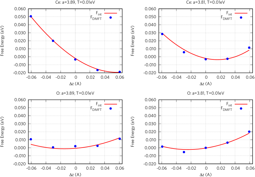
Figure 1: Energy profiles (blue points) in Ce₂O₃ when displacing Ce (top row) and O (bottom row) along $z$ direction. Left column corresponds to $a=3.89$ Å, while right column corresponds to $a=3.81$Å. The red curves correspond to the free energy profiles derived from integrating the analytical DFT+DMFT forces.

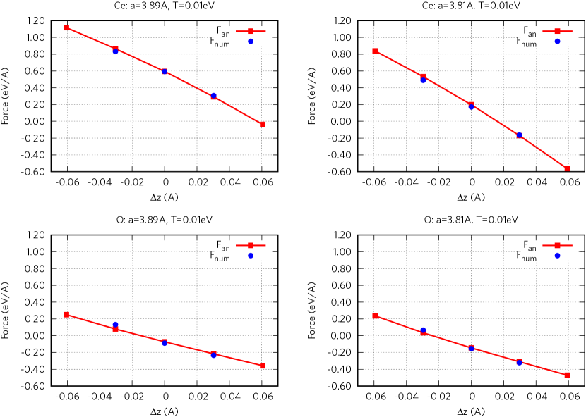
Figure 2: Comparison of the DFT+DMFT forces. Red points: analytical forces; blue points: numerical derivative extracted from the numerical free energy profiles reported in Fig.1. Forces acting on Ce (top row) and O (bottom row) along $z$ direction. Left column corresponds to $a=3.89$ Å, while right column corresponds to $a=3.81$ Å.

The results presented in this section are obtained by implementing the formulas presented above within the DFT+DMFT method implemented previously(Plekhanov et al., 2018; Sheridan et al., 2019) in the widely used plane-wave DFT code CASTEP(Payne et al., 1992; Clark et al., 2005). In order to benchmark our formalism, we apply it to Cerium sesquioxide Ce₂O₃, which has been studied for a long time(Andersson et al., 2007; Fabris et al., 2005; Singh et al., 2006; Loschen et al., 2007). It is known to be an anti-ferromagnetic insulator with Néel temperature of $T_{N}=9$ K and a gap of $2.4$ eV. DFT+DMFT calculations in the literature normally address the high-temperature paramagnetic phase, so to benchmark our forces calculations we also set the temperature to $T=0.01$ eV. Ce₂O₃ crystallizes in a hexagonal unit cell with space group $P\bar{3}m1$. The experimental parameters for the unit cell are: $a=3.89$ Å and $c/a=1.557$, with the Wyckoff positions(Wyckoff, 1967): Ce $2d$ $\left(\frac{1}{3},\frac{2}{3},\xi\right)$, O $2d$ $(\frac{1}{3},\frac{2}{3},\eta)$, O $1a$ $(0,0,0)$, with $\xi=0.24543$ and $\eta=0.6471$. On the other hand DFT predicts $a=3.81$ Å  at the experimental ratio $c/a=1.557$ and experimental $\xi$ and $\eta$. We have performed calculations for both lattice constants $a=3.81$ Å (minimum energy for DFT+DMFT method) and $a=3.89$ Å (the experimental value), while maintaining the ratio $c/a=1.557$. We have used the norm-conserving Ce and O pseudopotential (NCP17 set), LDA exchange-correlation potential and a $31\times 31\times 17$ Monkhorst-Pack $k$-point mesh. We have also checked that similar results are obtained with the ultrasoft pseudopotentials too. The plane-wave basis cut-off was automatically determined to be $1012$ eV. The values of Hubbard $U$ and Hund $J$ parameters were chosen to be $U=6$ eV and $J=0.7$ eV respectively. The results for Ce₂O₃ density of states at the experimental geometry are shown our previous work(Plekhanov et al., 2018) and exhibit excellent agreement with the reference calculations of Ref. Pourovskii et al., 2007. As in our previous paper, the DMFT calculations were performed with the Hubbard I solver (the extensions to the other types of solvers e.g. Hubbard III Górski and Mizia (2009, 2011) can be done) with a fixed occupancy of $n=1$ per Ce atom (in the sense explained in Ref. Pourovskii et al., 2007) within the FLL double-counting scheme.

For the benchmark to be fair, we compare the analytical forces calculated within our formalism against the numerical ones obtained from finite increment derivative of the free energy. On the other hand, we also compare the numerical free energy profiles against the curves obtained from the spline integration of the analytical forces. For what regards the evaluation of the numerical forces, we first note that most internal atomic coordinates are fixed by symmetry. We vary the remaining coordinates, which are the $z$-coordinates of Ce $2d$ and O $2d$ atoms (the ones established from experiment). Obviously, the forces of the atoms related by symmetry are in turn related. During finite increment of relevant atomic coordinates, we tested several $\Delta z$ values, in order to be sure that the free energy varies linearly over the lengthscale of $\Delta z$. The results of these tests are shown in Fig.8 of Ref.Plekhanov et al., 2018, and in this work we fix $\Delta z=1\%$ in units of the $c$-dimension of the unit cell. The numerical forces were determined as follows:

$$\mathbf{F}_{z_{i}}=-\frac{\partial F_{tot}}{\partial z_{i}}.$$ (39)

In addition, we emphasize that the total free energy as a function of $\Delta z$ is a smooth differentiable function, thanks to the fact that both DFT (CASTEP) and DMFT subsystems in our calculations are well-behaved, giving small responses to small perturbations. In order to be consistent with the formalism developed in the previous Section, in the present work, the DFT+DMFT was self-consistently converged until the energy became stationary up to $10^{-6}$eV.

The comparison between the analytical forces, calculated within the formalism presented in the previous section, and the numerical forces, derived from the total free energy according to Eq. (39), is shown in Figs. 1,2. The energy profiles are presented in Fig. 1, while the forces comparison is illustrated in Fig. 2. The overall agreement appears to be very good, taking into account the inevitable numerical bias of the DFT+DMFT total free energy. The forces calculated within our formalism are correct for both Ce - correlated ion, and O - "uncorrelated ion", on which the dynamical force is identically zero. We note that the local minimum (where the force is zero) with respect to the Ce displacement along $z$-axis is approximately $+0.06$ Å  with respect to the experimental position for the $a=3.89$ Å  unit cell, while it is about $+0.017$ Å  for the $a=3.81$ Å  unit cell. In the case of O displacement, the order of magnitude of forces is smaller, while the minima positions are roughly $-0.02$ Å  for both unit cells considered. Compared to the DFT forces (Table II of Ref. Plekhanov et al., 2018), the Ce DFT+DMFT forces presented here are larger, while the O forces are smaller. Compared to the one-shot DFT+DMFT forces (same table of Ref. Plekhanov et al., 2018), the full charge self-consistency modifies significantly the resulting force: for Ce - increasing, while for O decreasing. We conclude, therefore, that the one-shot DFT+DMFT somehow overshoots the forces with respect to the full self-consistent DFT+DMFT. It was shown in the Ref. Pourovskii et al., 2007, that the full self-consistent DFT+DMFT gives somewhat better agreement with the experiment for the Ce₂O₃ equilibrium volume as compared to the one-shot DFT+DMFT, thanks to the spectral weight redistribution. In addition, the difference between the DFT and the DMFT forces is larger on the "correlated" ions, although the "uncorrelated" ones are also modified due to the fact that the density is distributed differently in DFT+DMFT with respect to DFT. On the other hand, we have checked that the total vector sum of all the forces acting on all the atoms in the unit cell is zero within both DFT and DFT+DMFT as it should be in equilibrium.

IV.2 Forces in praseodymium dioxide

In order to enforce the validity of our approach, we have benchmarked the DMFT forces in yet another system: praseodymium dioxide PrO₂. We consider PrO₂ in the rhombohedral unit cell (symmetry group $Fm\bar{3}m$) with $a=4.0482$ Å  and the following Wyckoff positions of the atoms: Pr at $(0,0,0)$ and two oxygen atoms at $(\frac{1}{4},\frac{1}{4},\frac{1}{4})$ and $(\frac{3}{4},\frac{3}{4},\frac{3}{4})$ respectively (Chiba et al., 2011; Andreeva et al., 1986). Here, we have used ultra-soft pseudopotentials for both Pr and O (C17 set), LDA exchange-correlation potential and a $25\times 25\times 25$ Monkhorst-Pack $k$-point mesh. The plane-wave basis cut-off was automatically determined to be $653$ eV. The values of Hubbard $U$ and Hund $J$ parameters were chosen to be $U=6$ eV and $J=0.7$ eV respectively. At the above Wyckoff positions, the net DFT+DMFT forces are zero due to symmetry and the finite forces appear if the corresponding atoms are pushed away from their positions. Since both Pr and O atoms are placed on the cubic cell diagonal, in doing the finite displacements it is important to conserve the $3$-fold axis along the diagonal. That is why in the present subsection, we have performed the finite displacements of the Pr atom along the $(111)$ direction. The free energy increment between two atomic positions $\mathbf{R}^{1}$ and $\mathbf{R}^{2}$ has then been estimated by using the following formula:

$$F_{tot}(\mathbf{R}^{2})-F_{tot}(\mathbf{R}^{1})=-\int_{\mathbf{R}^{1}}^{\mathbf{R}^{2}}\sum_{\mu}\mathbf{F}_{\mu}(\mathbf{R})\mathrm{d}\mathbf{R}_{\mu},$$ (40)

where $\mathbf{F}_{\mu}(\mathbf{R})$ is the $\mu$’s component of the force at the atomic position vector $\mathbf{R}$, while $\mathbf{R}_{\mu}$ is the $\mu$’s Cartesian coordinate of the displaced Pr atom. The excellent agreement between $\delta F_{tot}$ derived from the analytical forces and the free energy profiles calculated in the vicinity of the high-symmetry Wyckoff position of Pr atom is shown in Fig. 3. The forces appear to be symmetric with respect to the displacements of the atoms along the diagonal in the positive and negative directions off the exact Wyckoff positions and so does the free energy profile. We would like to point out that in the case of PrO₂ the order of magnitude of forces and energy increments associated with the atomic displacements are an order of magnitude smaller as compared to the Ce₂O₃ case, which required additional accuracy in deriving smooth free energy profile.

Figure 3: Energy profiles (blue points) in PrO₂ when displacing Pr atom along the $(111)$ direction. $\mathrm{F_{int}}$ stands for the spline-integrated forces along the displacement path, while $\mathrm{F_{DMFT}}$ stands for system’s free energy calculated at given atomic positions using full charge self-consistency.

V Conclusions

In conclusion, we have presented a formalism for analytic calculation of the atomic forces within the full charge self-consistent pseudopotential DFT+DMFT approach. Our approach extends that of the Ref. Haule and Pascut, 2016 by taking into account the non-local projections terms in the KS Hamiltonian, which depend implicitly on charge distribution and arise from the pseudization procedure. It inherits the useful properties of the DFT+Embedded DMFT functional(Haule and Pascut, 2016) and, in particular $\frac{\delta P}{\delta G}=0$, and, therefore, the terms most difficult to calculate cancel out from the final result. Plane-wave basis, employed within our implementation, greatly simplifies the formalism by avoiding calculation of the augmentation charges. Our formalism is implemented within the DMFT framework inside CASTEP ab-initio code, which in the past already allowed for precise total free energy calculations within DFT+DMFT(Plekhanov et al., 2018). Our approach is general and suitable for both norm-conserving and ultrasoft pseudopotentials. The pseudopotential approach has an advantage of speeding up the calculations with respect to the all-electron methods by considering the core electrons as frozen, while the ultra-soft pseudopotentials further speed up the calculations with respect to the norm-conserving pseudopotentials by relaxing the norm-conserving condition Vanderbilt (1990); Laasonen et al. (1993).

In addition, our approach does not use any specific DMFT solver property and, hence, would work equally well with all solvers. We have presented the benchmark of our approach on the example of Ce₂O₃, which showed excellent agreement between the forces analytically calculated within our approach and the forces obtained from numerical differentiation of the total free energy at very low temperature. In addition, we have compared the total free energy profiles against the integrated forces profiles which also showed excellent agreement. We analyzed the differences of atomic forces within DFT, one-shot DFT+DMFT and full charge self-consistent DFT+DMFT on the examples of Ce₂O₃ and PrO₂, the applicability to the correlated metal close to the Mott transition being subject of our future studies. Our approach allows for quick and reliable force calculations within fully self-consistent pseudopotential DFT+DMFT and paves the way to the structural optimization, phonon and molecular dynamics calculations within DFT+DMFT.

Appendix A Calculation of the free energy

We start from Eq. (29) for the total free energy. We also report for completeness the formula for the total internal energy, used e.g. in our past work Plekhanov et al. (2018) (taking into account the ion-ion interaction energy):

$$E =\sum\varepsilon_{\mathbf{k},\nu}N_{\nu,\nu}(\mathbf{k})+E_{H}-\mathbf{\mathrm{Tr}}\left(V_{H}\rho\right)+E_{xc}-\mathrm{\mathbf{\mathrm{Tr}}}\left(V_{xc}\rho\right)$$

$$+\frac{1}{2}\mathrm{Tr}\Sigma G-\sum_{I}\Phi^{\mathrm{DC}}[G]+U(\mathbf{R}),$$ (41)

where $N_{\nu,\nu}(\mathbf{k})=T\sum_{n}G(\mathbf{k},i\omega_{n})$ is the DMFT occupancy matrix and $\varepsilon_{\mathbf{k},\nu}$ are the DFT eigenvalues calculated at the DMFT density. With respect to the total internal energy calculation, the changes are the following:

• The term $\sum\varepsilon_{\mathbf{k},\nu}N_{\nu,\nu}(\mathbf{k})$ is substituted with the following expression:

  $$\mathrm{Tr}\ln\hat{G}+\boldsymbol{\mu}\mathcal{N}-\mathrm{Tr}\left(\Sigma-V^{DC}\right)G;$$ (42)

• The term $\frac{1}{2}\mathrm{Tr}\Sigma G$ is substituted with:

  $$\Phi^{\mathrm{DMFT}}=F_{imp}-\mathrm{Tr}\ln G_{imp}+\mathrm{Tr}\Sigma_{imp}G_{imp}.$$ (43)

The calculation of the $\mathrm{Tr}\ln G$ with a general Green function $G$ is performed following the procedure outlined in the Ref. Haule and Birol, 2015, namely: the summation is split into two parts - numerical sum up to a cutoff Matsubara frequency $i\omega_{c}$ with the most divergent part subtracted, and an expression equal to the known analytical sum of the most divergent part. In this case, the most divergent part is:

$$\left.-T\sum_{n}\ln(-i\omega_{n}+\varepsilon)e^{i\eta\omega_{n}}\right|_{\eta\to 0}=-T\ln\left(1+e^{-\frac{\varepsilon}{T}}\right).$$ (44)

Therefore, the summation $\mathrm{Tr}\ln\hat{G}$ is evaluated as follows:

$$\mathrm{Tr}\ln\hat{G} =-T\sum_{\begin{subarray}{c}|\omega_{n}|<\omega_{c}\\ \mathbf{k}\end{subarray}}\mathfrak{Tr}\left\{\ln\left(-i\omega_{n}+\varepsilon_{\mathbf{k},\nu}-\boldsymbol{\mu}+\Sigma^{B}_{\nu,\nu^{\prime}}(\mathbf{k},i\omega_{n})-V_{\nu,\nu^{\prime}}^{DC}\right)-\ln\left(-i\omega_{n}+\varepsilon_{\nu,\nu^{\prime}}(\mathbf{k},\infty)\right)\right\}$$ (45)

$$-T\sum_{\mathbf{k}}\ln\left(1+\exp\left({-\frac{\varepsilon_{\nu,\nu^{\prime}}(\mathbf{k},\infty)}{T}}\right)\right),$$ (46)

where $\varepsilon_{\nu,\nu^{\prime}}(\mathbf{k},\infty)=\varepsilon_{\mathbf{k},\nu}-\boldsymbol{\mu}+\Sigma^{B}_{\nu,\nu^{\prime}}(\mathbf{k},\infty)-V_{\nu,\nu^{\prime}}^{DC}$.

On the other hand, the summation $\mathrm{Tr}\ln G_{imp}$ is evaluated as:

$$\mathrm{Tr}\ln G_{imp} =-T\sum_{|\omega_{n}|<\omega_{c}}\mathfrak{Tr}\left\{\ln\left(-i\omega_{n}+\varepsilon^{imp}_{m,m^{\prime}}+\Sigma^{imp}_{m,m^{\prime}}(i\omega_{n})\right)-\ln\left(-i\omega_{n}+\varepsilon^{imp}_{m,m^{\prime}}(\infty)\right)\right\}$$ (47)

$$-T\ln\left(1+\exp\left(-\frac{\varepsilon^{imp}_{m,m^{\prime}}(\infty)}{T}\right)\right),$$ (48)

where this time $\varepsilon^{imp}_{m,m^{\prime}}(\infty)=\varepsilon^{imp}_{m,m^{\prime}}+\Sigma^{imp}_{m,m^{\prime}}(\infty)$. Here, the notation $\mathfrak{Tr}$ stands for the trace over $\nu,\nu^{\prime}$ or $m,m^{\prime}$ indices respectively (without the summation over Matsubara frequencies).

Appendix B The use of the time reversal symmetry in the Matsubara sums

When doing the sums like $-\mathrm{Tr}\Sigma(i\omega_{n})G(i\omega_{n})$, one usually makes use of the symmetry properties of $\Sigma$ and $G$ upon changing $i\omega_{n}\to-i\omega_{n}$:

$$G_{m,m^{\prime}}(-i\omega_{n}) =G_{m^{\prime},m}^{\star}(i\omega_{n})$$

$$\Sigma_{m,m^{\prime}}(-i\omega_{n}) =\Sigma_{m^{\prime},m}^{\star}(i\omega_{n}),$$

so that

$$-T\sum_{n,m,m^{\prime}}\Sigma_{m,m^{\prime}}(-i\omega_{n})G_{m^{\prime},m}(-i\omega_{n})=$$

$$-T\sum_{n,m,m^{\prime}}G_{m,m^{\prime}}^{\star}(i\omega_{n})\Sigma_{m^{\prime},m}^{\star}(i\omega_{n})$$

hence:

$$-T\sum_{n,m,m^{\prime}}G_{m,m^{\prime}}(i\omega_{n})\Sigma_{m^{\prime},m}(i\omega_{n})=$$

$$-2T\mathrm{Re}\sum_{m,m^{\prime},\omega_{n}>0}G_{m,m^{\prime}}(i\omega_{n})\Sigma_{m^{\prime},m}(i\omega_{n}).$$

Considering the definition of $\Xi(i\omega_{n})$ given by the Eq. (34), we see that indeed:

$$\Xi_{m,m^{\prime}}(-i\omega_{n})=\Xi_{m^{\prime},m}^{\star}(i\omega_{n}).$$

Therefore, one can still use the Green function’s symmetry properties and restrict the summation in Eq. (33) to the positive Matsubara frequencies, while the final formula for the DFT+DMFT forces is given by the Eq. (32).

References

- Kotliar and Vollhardt (2004) G. Kotliar and D. Vollhardt, Physics Today 57, 53 (2004).
- Weber et al. (2012) C. Weber, D. D. O’Regan, N. D. M. Hine, M. C. Payne, G. Kotliar, and P. B. Littlewood, Phys. Rev. Lett. 108, 256402 (2012).
- Weber et al. (2013) C. Weber, D. D. O’Regan, N. D. M. Hine, P. B. Littlewood, G. Kotliar, and M. C. Payne, Phys. Rev. Lett. 110, 106402 (2013).
- Plekhanov et al. (2003) E. Plekhanov, S. Sorella, and M. Fabrizio, Phys. Rev. Lett. 90, 187004 (2003).
- Plekhanov et al. (2005) E. Plekhanov, F. Becca, and S. Sorella, Phys. Rev. B 71, 064511 (2005).
- Dai (2015) P. Dai, Rev. Mod. Phys. 87, 855 (2015).
- Joy et al. (2014) L. K. Joy, S. S. Samatham, S. Thomas, V. Ganesan, S. Al-Harthi, A. Liebig, M. Albrecht, and M. R. Anantharaman, Journal of Applied Physics 116, 213701 (2014).
- Babulanam et al. (1987) S. Babulanam, T. Eriksson, G. Niklasson, and C. Granqvist, Solar Energy Materials 16, 347 (1987).
- Granqvist (1990) C. Granqvist, Thin Solid Films 193-194, 730 (1990).
- Granqvist (2007) C. G. Granqvist, Solar Energy Materials and Solar Cells 91, 1529 (2007).
- Tomczak and Biermann (2009) J. M. Tomczak and S. Biermann, Europhysics Letters 86, 37004 (2009).
- Georges et al. (1996) A. Georges, G. Kotliar, W. Krauth, and M. J. Rozenberg, Rev. Mod. Phys. 68, 13 (1996).
- Vollhardt (2010) D. Vollhardt, AIP Conference Proceedings 1297, 339 (2010).
- Savrasov and Kotliar (2004) S. Y. Savrasov and G. Kotliar, Phys. Rev. B 69, 245101 (2004).
- Minár et al. (2005) J. Minár, L. Chioncel, A. Perlov, H. Ebert, M. I. Katsnelson, and A. I. Lichtenstein, Phys. Rev. B 72, 045125 (2005).
- Kotliar et al. (2006) G. Kotliar, S. Y. Savrasov, K. Haule, V. S. Oudovenko, O. Parcollet, and C. A. Marianetti, Rev. Mod. Phys. 78, 865 (2006).
- Pourovskii et al. (2007) L. V. Pourovskii, B. Amadon, S. Biermann, and A. Georges, Phys. Rev. B 76, 235101 (2007).
- Amadon et al. (2008) B. Amadon, F. Lechermann, A. Georges, F. Jollet, T. O. Wehling, and A. I. Lichtenstein, Phys. Rev. B 77, 205112 (2008).
- Amadon (2012) B. Amadon, Journal of Physics: Condensed Matter 24, 075604 (2012).
- Koçer et al. (2020) C. P. Koçer, K. Haule, G. L. Pascut, and B. Monserrat, Phys. Rev. B 102, 245104 (2020).
- Plekhanov et al. (2018) E. Plekhanov, P. Hasnip, V. Sacksteder, M. Probert, S. J. Clark, K. Refson, and C. Weber, Phys. Rev. B 98, 075129 (2018).
- Sheridan et al. (2019) E. Sheridan, C. Weber, E. Plekhanov, and C. Rhodes, Phys. Rev. B 99, 205156 (2019).
- McMahon et al. (2019) M. I. McMahon, S. Finnegan, R. J. Husband, K. A. Munro, E. Plekhanov, N. Bonini, C. Weber, M. Hanfland, U. Schwarz, and S. G. Macleod, Phys. Rev. B 100, 024107 (2019).
- Pace et al. (2020) E. J. Pace, S. E. Finnegan, C. V. Storm, M. Stevenson, M. I. McMahon, S. G. MacLeod, E. Plekhanov, N. Bonini, and C. Weber, Phys. Rev. B 102, 094104 (2020).
- Haule and Birol (2015) K. Haule and T. Birol, Phys. Rev. Lett. 115, 256402 (2015).
- Savrasov and Kotliar (2003) S. Y. Savrasov and G. Kotliar, Phys. Rev. Lett. 90, 056401 (2003).
- Leonov et al. (2014) I. Leonov, V. I. Anisimov, and D. Vollhardt, Phys. Rev. Lett. 112, 146401 (2014).
- Haule and Pascut (2016) K. Haule and G. L. Pascut, Phys. Rev. B 94, 195146 (2016).
- Georges (2004) A. Georges, AIP Conference Proceedings 715, 3 (2004).
- Haule (2015) K. Haule, Phys. Rev. Lett. 115, 196403 (2015).
- Vanderbilt (1990) D. Vanderbilt, Phys. Rev. B 41, 7892 (1990).
- Laasonen et al. (1993) K. Laasonen, A. Pasquarello, R. Car, C. Lee, and D. Vanderbilt, Phys. Rev. B 47, 10142 (1993).
- Martin (2004) R. M. Martin, Electronic Structure: Basic Theory and Practical Methods (Cambridge University Press, 2004).
- Himmetoglu et al. (2014) B. Himmetoglu, A. Floris, S. de Gironcoli, and M. Cococcioni, International Journal of Quantum Chemistry 114, 49 (2014).
- Timrov et al. (2020) I. Timrov, F. Aquilante, L. Binci, M. Cococcioni, and N. Marzari, Phys. Rev. B 102, 235159 (2020).
- Payne et al. (1992) M. C. Payne, M. P. Teter, D. C. Allan, T. Arias, and J. D. Joannopoulos, Rev. Mod. Phys. 64, 1045 (1992).
- Clark et al. (2005) S. J. Clark, M. D. Segall, C. J. Pickard, P. J. Hasnip, M. J. Probert, K. Refson, and M. Payne, Z. Kristall. 220, 567 (2005).
- Andersson et al. (2007) D. A. Andersson, S. I. Simak, B. Johansson, I. A. Abrikosov, and N. V. Skorodumova, Phys. Rev. B 75, 035109 (2007).
- Fabris et al. (2005) S. Fabris, S. de Gironcoli, S. Baroni, G. Vicario, and G. Balducci, Phys. Rev. B 71, 041102 (2005).
- Singh et al. (2006) N. Singh, S. M. Saini, T. Nautiyal, and S. Auluck, Journal of Applied Physics 100, 083525 (2006).
- Loschen et al. (2007) C. Loschen, J. Carrasco, K. M. Neyman, and F. Illas, Phys. Rev. B 75, 035115 (2007).
- Wyckoff (1967) R. W. G. Wyckoff, Crystal Structures, 2nd ed., Vol. 2 (Interscience, New York, 1967) p. 1.
- Górski and Mizia (2009) G. Górski and J. Mizia, Phys. Rev. B 79, 064414 (2009).
- Górski and Mizia (2011) G. Górski and J. Mizia, Phys. Rev. B 83, 064410 (2011).
- Chiba et al. (2011) R. Chiba, H. Taguchi, T. Komatsu, H. Orui, K. Nozawa, and H. Arai, Solid State Ionics 197, 42 (2011).
- Andreeva et al. (1986) A. Andreeva, I. Gil’man, M. Gamarnik, and V. Dekhtyaruk, Izvestiya Akademii Nauk SSSR, Metally 1986, 1155 (1986).