Phase-space interpretation of spatial stationarity for coherence holography

Abstract

We extend the wide-sense spatial stationarity concept of coherence holography in the regime of phase-space using the wigner distribution function. We focus mainly on the incoherent light source and the Fourier and Fresnel propagation kernels for the optical-field transformation rule (input-output relation) and derive the same analogy in WDF. We further show that in phase-space the WDF obtained from the ensemble-averaged and space-averaged coherence functions are the same. Finally, we interpret behaviour of these results through numerical simulations.

I introduction

In 1932, E. Wigner introduced the Wigner distribution function (WDF) to analyse quantum mechanical systems in phase-space [23]. Later, Ville [7, 17] and Bastiaans [2, 5, 6] introduced this concept in Signal processing and Fourier optics, respectively. Since then, it has found numerous applications as being an excellent tool for the phase-space analysis with many properties [3, 22]. However, any of these property’s applicability depends on the analysis being done. For example, being a bilinear function, it produces undesirable cross-WDF terms for some Holography and Signal processing applications [18, 10].

In the past, there have been several publications on phase space interpretation of Holography. For example, Lohmann et al. proposed a Wigner chart method to examine the hologram recording materials and detectors’ storage capacity, which is an easy way to determine recording trade-off for various Hologram recording schemes [14]. Likewise, Oh and Barbastath presented a way to obtain WDF of the volume hologram. To produce the result, they first got the WDF of the 4f imager and then used the WDF shearing properties [15]. Next, Kim, Hwi, et al. proposed an optical sectioning method for optical sectioning holography. They showed that the focused and defocused information at the focal plane are separable in phase-space (WDF); hence, a filter mechanism can be built [11]. Likewise, one may find examples of varied applications of the WDF in Holography.

Holography is a widely used principle in optical and non-optical applications. It was first introduced by Gabor in 1948 as a microscopic principle to record complete information (phase and amplitude) of an object [8]. Later, Leith and Upatneiks modified this principle by introducing the off-set reference wave [12, 13]. Since then, many conventional and non-conventional Holography techniques have been reported. One such non-conventional holography technique is the Coherence Holography proposed by Takeda et al. In this technique, the hologram is recorded with coherent light and reconstructed with incoherent light. The resulting image, upon reconstruction, is the distribution of spatial coherence function, obtained from the space average instead of the ensemble average. To further elaborate, we deal with spatial statistics of an optical field rather than its temporal statistics. If a statistical field is temporally stationary and ergodic, then the ensemble average is replaced by the time average. Usually, the coherence function is obtained from the ensemble average or time average, which is applicable for many practical cases. Nonetheless, modern advances in optics such as time-frozen optical fields can not be dealt with temporal statistics and motivates us to devise other methods as well. This is where the spatial statistics comes into the picture. When scattered from a diffusive material, such fields give a good insight into the object when dealt with spatial statistics. Although not much has been explored into the spatial statistical approach, the coherence holography elaborates an excellent use of it by replacing the ensemble average by the space average provided the wide-sense spatial staionarity condition is satisfied [20, 19, 21, 16]. In this letter, our attempt is to interpret this condition in phase-space and to supplement the underlying theory of coherence holography. Our primary focus here is the reconstruction with the Fourier and Fresnel kernels and the source obtained from the hologram illuminated with incoherent light. Now, as we proceed section-wise, we will elaborate more onto each concept.

Sec. 2. has three subsections A, B, and C. In A, we derive the input-output relation of the WDF for partially coherent light and introduce the double WDF concept. In B, we present the conditions for the validity of wide-sense spatial stationarity of the output coherence function. Then, we derive the Wigner counterparts of the input coherence function (from the source) and the Fourier and Fresnel kernels. Finally, in C., we present an alternative way to obtain the output WDFs from the spatial coherence functions. Next in sec. 3., we demonstrate simulated results and infer the behaviour of output WDFs and their relation to the input WDFs. Finally, in sec. 4., we conclude with some remarks on our result.

II theory

II.1 Input-ouput relation

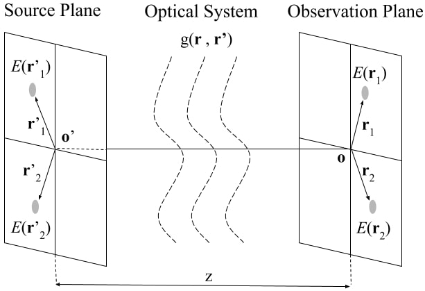
Figure 1: Geometry of source plane, optical system, and observation plane.

Let us consider an input-output relation for an optical field, which is coherent and quasi-monochromatic in nature.

$$E\left(\bm{r}\right)=\int g\left(\bm{r},\bm{r}^{\prime}\right)E\left(\bm{r}^{\prime}\right)dr^{\prime}$$ (1)

As shown in fig. 1, $E\left(\bm{r}\right)$ and $E\left(\bm{r}^{\prime}\right)$ are the optical fields at the source $\left(\bm{r}^{\prime}\right)$ and observation $\left(\bm{r}\right)$ planes, respectively. The function $g\left(\bm{r}^{\prime},\bm{r}\right)$ is the line-spread function or green’s function, describing the impulse-response relation of the system. Also, the integration is taken over the entire source plane unless otherwise stated. Now, if the light is partially coherent, the field becomes a stochastic process, and its transformation is studied in terms of coherence function or two-point correlation function. The coherence function is defined as $\Gamma\left(\bm{r}_{1},\bm{r}_{2}\right)=\left\langle E^{*}\left(\bm{r}_{1}\right)E\left(\bm{r}_{2}\right)\right\rangle$, where $E\left(\bm{r}\right)$ is the field and $\left\langle...\right\rangle$ represents the ensemble average. One may easily derive the input-output relation in terms of coherence function by using Eq. $(1)$ for $E\left(\bm{r}\right)$. This input-output relation has an analogy in terms of WDF as well [22].

For that, we first consider the WDF definition of the input coherence function (at the source plane),

$$\mathcal{W}\left(\bm{q}^{\prime},\bm{k}^{\prime}\right)=\frac{1}{2\pi}\int\Gamma\left(\bm{q}^{\prime}-\frac{\bm{p}^{\prime}}{2},\bm{q}^{\prime}+\frac{\bm{p}^{\prime}}{2}\right)\exp\left\{-i\bm{k}^{\prime}\cdot\bm{p}^{\prime}\right\}d\bm{p}^{\prime}$$ (2)

It also implies the following inverse WDF relation

$$\Gamma\left(\bm{q}^{\prime}-\frac{\bm{p}^{\prime}}{2},\bm{q}^{\prime}+\frac{\bm{p}^{\prime}}{2}\right)=\int\mathcal{W}\left(\bm{q}^{\prime},\bm{k}^{\prime}\right)\exp\left\{i\bm{k}^{\prime}\cdot\bm{p}^{\prime}\right\}d\bm{k}^{\prime}$$ (3)

Next, we consider the double WDF definition, which is a basic definition for our analysis.

$$\mathcal{G}\left(\bm{q},\bm{k},\bm{q}^{\prime},\bm{k}^{\prime}\right)=\frac{1}{2\pi}\iint g^{*}\left(\bm{q}-\frac{\bm{p}}{2},\bm{q}^{\prime}-\frac{\bm{p}^{\prime}}{2}\right)$$

$$...\times g\left(\bm{q}+\frac{\bm{p}}{2},\bm{q}^{\prime}+\frac{\bm{p}^{\prime}}{2}\right)\exp\left\{-i\left(\bm{k}\cdot\bm{p}-\bm{k}^{\prime}\cdot\bm{p}^{\prime}\right)\right\}d\bm{p}d\bm{p}^{\prime}$$ (4)

Together with Eq. (3) and (4), when we evaluate the WDF of the output coherence function using Eq. (1), we obtain the WDF input-output relation.

$$\mathcal{W}\left(\bm{q},\bm{k}\right)=\iint\mathcal{G}\left(\bm{q},\bm{k},\bm{q}^{\prime},\bm{k}^{\prime}\right)\mathcal{W}\left(\bm{q}^{\prime},\bm{k}^{\prime}\right)d\bm{q}^{\prime}d\bm{k}^{\prime}$$ (5)

where $\bm{q}$ and $\bm{k}$ are the space and spatial-frequency variables, respectively. For simplicity, we have explicitly excluded the temporal dependence. Also, In this letter, we have used the following change of variables whenever applicable.

$$\begin{array}[]{ccc}\mathrm{output}&&\mathrm{input}\\ \bm{r}_{1}=\bm{q}-\bm{p}/2&\quad\&&\bm{r}^{\prime}_{1}=\bm{q}^{\prime}-\bm{p}^{\prime}/2\\ \bm{r}_{2}=\bm{q}+\bm{p}/2&&\bm{r}^{\prime}_{2}=\bm{q}^{\prime}+\bm{p}^{\prime}/2\end{array}$$ (6)

II.2 Incoherent light and Ensemble average

Incoherent light source

The results that we have obtained are generic, i.e., without any specific assumption. However, in the coherence holography, it is required that the output coherence function is wide-sense spatial stationary. This stationarity condition is crucial for replacing the ensemble average by the space average. So, if we assume that the source is wide-sense stationary, i.e., $\Gamma\left(\bm{r}^{\prime}_{1}+\bm{r}_{s},\bm{r}^{\prime}_{2}+\bm{r}_{s}\right)=\Gamma\left(\bm{r}^{\prime}_{1},\bm{r}^{\prime}_{2}\right)$ and the green’s function is shift-invariant, i.e., $g\left(\bm{r}^{\prime}+\bm{r}_{s},\bm{r}+\bm{r}_{s}\right)=g\left(\bm{r}^{\prime},\bm{r}\right)$ for a unit magnification $\left(\bm{r}_{s}=\bm{r}^{\prime}_{s}\right)$. The output coherence function becomes wide-sense stationary, verified from the input-output relation for coherence function. But, in the coherence holography, the source is obtained from illuminating the hologram by spatially incoherent light. This is practically achieved by passing the Laser light through rotating ground glass. The desired ensemble-averaged degree of spatial coherence can be explicitly controlled by several factors, given elsewhere [1]. The ensemble-averaged input coherence function becomes $\Gamma\left(\bm{r}^{\prime}_{1},\bm{r}^{\prime}_{2}\right)=\mathrm{I}\left(\bm{r}^{\prime}_{1}\right)\delta\left(\bm{r}^{\prime}_{2}-\bm{r}^{\prime}_{1}\right)$, where $\mathrm{I}\left(\bm{r}^{\prime}_{1}\right)$ is made proportional to the intensity transmittance of the Hologram. It generally has a complicated spatial fringe structure with limited spatial extent, which means that such a source of practical interest is typically non-stationary. Even though with a suitable propagation kernel the output coherence function can still be made wide-sense stationary. Two such green’s functions are Fourier and Fresnel kernels [20, 19, 21].

Now, for our analysis, we require an input WDF obtained from input coherence function. So, if we put the above-defined coherence function in Eq. (2), we get the following WDF,

$$\mathcal{W}\left(\bm{q}^{\prime},\bm{k}^{\prime}\right)=\mathrm{I}\left(\bm{q}^{\prime}\right)$$ (7)

As can be seen in Eq. $\left(7\right)$ that the input WDF is a function of space variable only, which means the light radiates equally in all directions (with $\mathrm{I}\left(\bm{q}^{\prime}\right)\geq 0$) [4].

Fourier kernel

We consider a 2D Fourier kernel [9] which is defined as

$$g\left(\bm{r},\bm{r^{\prime}}\right)=\frac{-ik_{o}}{2\pi f}\exp\left(ik_{o}f\right)\exp\left(-ik_{o}\frac{\bm{r}\cdot\bm{r}^{\prime}}{f}\right)$$ (8)

where $k_{\circ}$ is the mean wavenumber of the quasimonochromatic light, and $f$ is the focal length of an aberration-free lens. Also, the lens is assumed to be large enough so that the finite-aperture effects can be neglected. The variables $\bm{r}$ and $\bm{r}^{\prime}$ in the green’s function have usual meaning. Now if we put Eq. $\left(8\right)$ in the double WDF formula, that is Eq. $\left(4\right)$, we obtain the following double WDF of the Fourier kernel

$$\mathcal{G}_{\mathrm{fourier}}\left(\bm{q},\bm{k},\bm{q}^{\prime},\bm{k}^{\prime}\right)=\frac{1}{2\pi}\iint\exp\left\{i\frac{k_{o}}{f}\left(\bm{q}-\frac{\bm{p}}{2}\right)\cdot\left(\bm{q}^{\prime}-\frac{\bm{p}^{\prime}}{2}\right)\right\}\times\exp\left\{-i\frac{k_{o}}{f}\left(\bm{q}+\frac{\bm{p}}{2}\right)\cdot\left(\bm{q}^{\prime}+\frac{\bm{p}^{\prime}}{2}\right)\right\}\mathrm{e}^{-i\left(\bm{k}\cdot\bm{p}-\bm{k}^{\prime}\cdot\bm{p}^{\prime}\right)}d\bm{p}d\bm{p}^{\prime}$$

$$=\frac{k_{o}}{2\pi f}\delta\left(\bm{q}^{\prime}+\frac{f\bm{k}}{k_{o}}\right)\delta\left(\bm{k}^{\prime}-\frac{k_{o}\bm{q}}{f}\right)$$ (9)

Again, from Eq. $\left(7\right)$ and Eq. $\left(9\right)$, we obtain the final output WDF using Eq. $\left(5\right)$

$$\mathcal{W}\left(\bm{q},\bm{k}\right)=\frac{k_{o}}{2\pi f}\mathrm{I}\left(-\frac{f\bm{k}}{k_{o}}\right)$$ (10)

The output WDF in Eq. $\left(10\right)$, apart from a constant factor, has the same intensity profile as that of the input WDF in Eq. $\left(5\right)$. It is also a function of spatial-frequency only, which implies that it has rotated in phase-space by $\pi/2$ radians in magnitude, and the minus sign indicates the intensity profile flip. It should be noted that the above formalism works well for the 1D case as well, i.e., with scalar variables, when replacing the ensemble average by the space average. However, the same isn’t the case for the Fresnel kernel mentioned below.

Fresnel kernel

Here, we consider a 2-D Fresnel kernel. This formalism is only applicable for the 2D case for a reason given elsewhere [21, 19] and will also be evident when we cover the next section on space average. The Fresnel kernel reads [9]

$$g\left(\bm{r},\bm{r}^{\prime}\right)=\frac{-ik_{o}}{2\pi z}\mathrm{e}^{ik_{o}z}\exp\left\{-i\frac{k_{o}}{2z}\left(\left|\bm{r}\right|^{2}-2\bm{r}\cdot\bm{r}^{\prime}+\left|\bm{r}^{\prime}\right|^{2}\right)\right\}$$ (11)

where $z$ is the distance between the source and the observation planes, and the other symbols have their usual meanings. Now, putting the Eq. $\left(11\right)$ in $\left(4\right)$ would yield the following double WDF of the Fresnel kernel

$$\mathcal{G}_{\mathrm{fresnel}}\left(\bm{q},\bm{k},\bm{q}^{\prime},\bm{k}^{\prime}\right)=\frac{1}{2\pi}\left(\frac{k_{o}}{2\pi z}\right)^{2}\iint\exp\left\{i\frac{k_{o}}{2z}\left[\left|\bm{q}-\frac{\bm{p}}{2}\right|^{2}-2\left(\bm{q}-\frac{\bm{p}}{2}\right)\cdot\left(\bm{q}^{\prime}-\frac{\bm{p}^{\prime}}{2}\right)+\left|\bm{q}^{\prime}-\frac{\bm{p}^{\prime}}{2}\right|^{2}\right]\right\}$$

$$...\times\exp\left\{-i\frac{k_{o}}{2z}\left[\left|\bm{q}+\frac{\bm{p}}{2}\right|^{2}-2\left(\bm{q}+\frac{\bm{p}}{2}\right)\cdot\left(\bm{q}^{\prime}+\frac{\bm{p}^{\prime}}{2}\right)+\left|\bm{q}^{\prime}+\frac{\bm{p}^{\prime}}{2}\right|^{2}\right]\right\}\exp\left[-i\left(\bm{k}\cdot\bm{p}-\bm{k}^{\prime}\cdot\bm{p}^{\prime}\right)\right]d\bm{p}d\bm{p}^{\prime}$$

$$=\frac{k_{o}}{2\pi z}\delta\left(\bm{q}^{\prime}-\left\{\bm{q}+\frac{z\bm{k}}{k_{o}}\right\}\right)\delta\left(\bm{k}^{\prime}-\frac{k_{o}}{z}\left\{\bm{q}-\bm{q}^{\prime}\right\}\right)$$ (12)

and from the Eq. $\left(7\right)$ and Eq. $\left(12\right)$ the output WDF using the Eq. $\left(5\right)$ becomes

$$\mathcal{W}\left(\bm{q},\bm{k}\right)=\frac{k_{o}}{2\pi z}\mathrm{I}\left(\bm{q}+\frac{z\bm{k}}{k_{o}}\right)$$ (13)

Here also the output WDF, apart from a constant factor, has the same intensity profile as given in Eq. $\left(7\right)$. Nevertheless, the input WDF rotates in the phase-space such that the intensity profile is defined on a hyperplane given by $\bm{q}+z\bm{k}/k_{\circ}=arbitrary\>constant$, i.e., it rotates in the phase-space according to the value $z/k_{o}$ or how far the field propagates in fresnel regime.

Figure 2: (a) & (e) are respectively the 2D and 3D plots of the intensity transmittance of the Fourier hologram illuminated by a plane wave at some angle; (b) & (f) are respectively the output WDFs for a particular values of ($y,k_{y}$) and ($x,k_{x}$) in case of Fourier kernel; (c) & (g) are respectively the output WDFs for a particular values of ($y,k_{y}$) and ($x,k_{x}$) in case of Fresnel kernel. Plots (i), (j), & (k) are respectively the 1D intensity profile, vertical cross-section of its WDF along $k_{x}$-axis, and the entire WDF itself.

II.3 Space average

Spatial coherence function & WDF

It is common to replace the ensemble average by the time average if the statistical field is ergodic and stationary in time. However, the same isn’t the case in spatial statistical approach. In most practical cases, neither the sources nor their diffraction fields are spatially stationary. But, as mentioned earlier, the Fourier and Fresnel kernels can produce wide-sense spatially stationary fields even though the sources are spatially non-stationary. Then it is possible to replace the ensemble average by the space average, which is defined differently as per the kernels used, i.e., both Fourier and Fresnel kernels would have different space averaging definitions. These results are well established and given elsewhere [19, 21]. Here, we present the phase-space interpretation of these replacements. Also, one may find the following derivations in the paper mentioned above. Still, for consistency, we have shown the steps explicitly and then implemented the WDF analogy of those results.

Let us consider the definition of (output) spatial coherence function [21, 19]

$$\Gamma^{s}\left(\bm{p}\right)=\int E^{*}\left(\bm{q}-\frac{\bm{p}}{2}\right)E\left(\bm{q}+\frac{\bm{p}}{2}\right)d\bm{q}$$ (14)

where the field $E$ is given by Eq. $\left(1\right)$, the superscript $s$ stands for the space average, and the variables are as per the Eq. $\left(6\right)$. Here in Eq. $\left(14\right)$, the ensemble average is replaced by the space average in the definition of coherence function. This replacement is valid if the coherence function is wide-sense stationary [16]. Correspondingly, the output WDF is given by

$$\mathcal{W}^{s}\left(\bm{k}\right)=\int\Gamma^{s}\left(\bm{p}\right)\exp\left\{-i\bm{k}\cdot\bm{p}\right\}d\bm{p}$$ (15)

Next, we derive WDF of the spatial coherence functions for the Fourier and Fresnel kernels.

Fourier kernel

For a 2D Fourier kernel (Eq. $\left(8\right)$), if we use Eq. $\left(1\right)$ in Eq. $\left(14\right)$ and perform space averaging, we obtain

$$\Gamma^{s}\left(\bm{p}\right)=\frac{k_{o}}{2\pi f}\iint\exp\left\{-i\frac{k_{o}}{2f}\bm{p}\cdot(\bm{q}_{1}+\bm{q}_{2})\right\}\delta\left(\bm{q}_{1}-\bm{q}_{2}\right)$$

$$...\times E^{*}\left(\bm{q}_{1}\right)E\left(\bm{q}_{2}\right)d\bm{q}_{1}d\bm{q}_{2}$$

$$=\frac{k_{o}}{2\pi f}\int\mathrm{I}\left(\bm{q}_{1}\right)\exp\left(-i\frac{k_{o}}{f}\bm{q}_{1}\cdot\bm{p}\right)d\bm{q}_{1}$$ (16)

Now putting equation $\left(16\right)$ in equation $\left(15\right)$ yields

$$\mathcal{W}^{s}\left(\bm{k}\right)=\mathrm{I}\left(-\frac{f\bm{k}}{k_{o}}\right)$$ (17)

where $\mathrm{I}\left(\bm{q}_{1}\right)=E^{*}\left(\bm{q}_{1}\right)E\left(\bm{q}_{1}\right)$ is the instantaneous intensity distribution over the source plane. Eq. $(17)$ is the WDF of the output spatial coherence function obtained from Fourier kernel. Also, note that the expression obtained in equation $\left(17\right)$ is equivalent to equation $\left(10\right)$.

Fresnel kernel

Again, in the case of 2D Fresnel kernel, we modify the spatial averaging definition by considereing $\bm{q}=\bm{q}_{\|}+\bm{q}_{\bot}$, where $\bm{q}_{\bot}$ and $\bm{q}_{\|}$ are the orthogonal components of $\bm{q}$ such that $\bm{q}_{\bot}$ is perpendicular to $\bm{p}$ ($\bm{q}_{\bot}$$\cdot\bm{p}=0$). Also we take space average with respect to $\bm{q}_{\bot}$ instead of $\bm{q^{\prime}}$ in equation $\left(14\right)$ [19, 21], i.e.,

$$\Gamma^{s}\left(\bm{q}_{\|},\bm{p}\right)=\iiint g^{*}\left(\bm{q}_{\bot}+\bm{q}_{\|}-\frac{\bm{p}}{2},\bm{q}_{1}\right)E^{*}\left(\bm{q}_{1}\right)$$

$$...\times g\left(\bm{q}_{\bot}+\bm{q}_{\|}+\frac{\bm{p}}{2},\bm{q}_{2}\right)E\left(\bm{q}_{2}\right)d\bm{q}_{1}d\bm{q}_{2}d\bm{q}_{\bot}$$ (18)

putting Eq. $\left(11\right)$ for the green’s function in Eq. $\left(18\right)$ and performing space average gives (after some algebraic steps)

$$\Gamma^{s}\left(\bm{q},\bm{p}\right)=\frac{k_{o}}{2\pi z}\exp\left(-i\frac{k_{o}}{z}\bm{p}\cdot\bm{q}_{\|}\right)\iint\delta\left(\bm{q}_{1}-\bm{q}_{2}\right)E^{*}\left(\bm{q}_{1}\right)E\left(\bm{q}_{2}\right)$$

$$...\times\exp\left[\frac{ik_{o}}{2z}\left\{2\bm{q}_{\|}\cdot(\bm{q}_{2}-\bm{q}_{1})+\bm{p}\cdot(\bm{q}_{2}+\bm{q}_{1})-(\bm{q}_{2}^{2}-\bm{q}_{1}^{2})\right\}\right]d\bm{q}_{1}d\bm{q}_{2}$$

$$=\frac{k_{o}}{2\pi z}\exp\left(-i\frac{k_{o}}{z}\bm{p}\cdot\bm{q}\right)\int\exp\left(i\frac{k_{o}}{z}\bm{p}\cdot\bm{q}_{1}\right)\mathrm{I}\left(\bm{q}_{1}\right)d\bm{q}_{1}$$ (19)

note that the substitution $\bm{p}\cdot\bm{q}_{\|}=\bm{p}\cdot\bm{q}$ is valid as $\bm{q}_{\bot}\cdot$$\bm{p}=0$. Now putting Eq. $\left(19\right)$ in Eq. $\left(15\right)$ gives the following output WDF of the modified spatial coherence function

$$\mathcal{W}^{s}\left(\bm{q},\bm{k}\right)=\mathrm{I}\left(\bm{q}+\frac{z\bm{k}}{k_{o}}\right)$$ (20)

Here as well the obtained WDF is equivalent to the Eq. $(13)$. Hence, one may get the output WDF from the spatial coherence functions instead of the ensemble-averaged coherence function if the wide-sense stationarity condition holds as discussed so far.

III Results and Discussion

Here are the simulation results of the WDFs obtained for the Fourier and Fresnel kernels. In Fig. $2$, (a) & (e) represent the 2D and 3D plots of the intensity transmittance of the Fourier hologram of a circular aperture illuminated by a plane wave at some angle to give fringe pattern as shown. Usually, this Airy pattern is generated by illuminating the hologram with the incoherent plane wave and then taking the ensemble average. However, as we have seen that the output coherence functions and the output WDFs are equivalent in the cases of ensemble average and space average given the conditions are satisfied, The Airy pattern here is simply generated by illuminating the hologram with the plane wave once. It serves as the instantaneous intensity profile for the spatial averaging approach. Also, it is to be noted that the fringes occur along the x-axis. Next, the figures (b) and (f) are the 2D WDFs obtained from the Fourier kernels. Although the output WDF would be 4D, for the sake of interpreting its behaviour, we have chosen a constant value of $(y,k_{y})$ in (b) where the normalized WDF is one. In our case, it is the intermediate values of y and ky of the image and its Fourier transform. As depicted from the Eq. $(10)$ and $(17)$ the input WDF rotates in the phase-space by $\pi/2$ radians in magnitude to give the output WDF. The minus sign in Eq. (10) or (17) represents an inversion of the intensify profile along k-axis. However, since the intensity profile in our WDF expression is symmetric, this behaviour is not apparent. Likewise, figure (f) shows the same behaviour but for the constant value of $(x,k_{x})$ where the normalized WDF value is one. Finally, figures (c) and (g) are the 2D WDFs obtained from the Fresnel kernel. Here as well, the plots are shown for constant values of $(y,k_{y})$ and $(x,k_{x})$ where the normalized WDF values are one, respectively. In Eq. $(13)$ and $(20)$, it is shown that the output WDF is the intensity profile with arguments as a linear combination of space and spatial-frequency variables, i.e., $\bm{q}+z\bm{k}/k_{\circ}$. It implies that the input WDF rotates in the phase-space according to the value of $z/k_{\circ}$ or how far the coherence function propagates in the Fresnel regime. In our case, we have simply taken this value equal to unity, i.e., $z/k_{\circ}=1\>m^{2}$. Therefore, in figures (c) and (g), the intensity profiles are defined on a hyperplane $\bm{q}+\bm{k}=arbitrary\>constant$. In other words, the input WDF rotates in phase-space by $\pi/4$ radians in magnitude. As mentioned earlier, the formalism for the Fourier kernel is also valid in 1D case. Figure (i) shows a 1D intensity profile obtained from the superposition of two Gaussian profiles with different amplitudes and shifted means. Also, the smaller amplitude Gaussian profile is to the left of the bigger one. In figures (j) and (k), the corresponding vertical cross-section of the WDF along $k_{x}$-axis and the entire WDF are shown, respectively. One may notice that apart from a $\pi/2$ rotation in phase-space, the intensity profiles in figures (j) and (k) are inverted, demonstrating the effect of minus sign in the output WDF (Eq. $(10)$ and $(17)$) obtained from the Fourier kernel.

IV Conclusion

s In this paper, we showed, by suplimenting the unlying theory of coherence holography, that in phase-space the output WDFs obtained from the ensemble-averaged and space-averaged cohererence functions are equivalent to each other provided the source in spatially incoherent and the propagation kernel is either Fourier or Fresnel. Also, in the case of Fresnel kernel, the space average definition is modified accordingly. We also showed the behaviours of these output WDFs in the phase-space. For the Fourier kernel, the WDF rotates in phase-space by $\pi/2$ radians in magnitude and the intensity profile is inverted; whereas, for the Fresnel kernel, the WDF rotates in phase-space depending on how far the coherence function propagates in the Fresnel regime, i.e., $z/k_{\circ}$ value. These results are in general valid for any optical phenomena where these conditions are statisfied. Hence, one may replace the output WDF obtained from ensemble-averaged coherence function by the WDF obtained from the space-averaged coherence function.