In-situ pseudopotentials for electronic structure theory

Abstract

We present a general method of constructing in-situ pseodopotentials from first principles, all-electron, full-potential electronic structure calculations of a solid. The method is applied to bcc Na, at equilibrium volume. The essential steps of the method involve (i) calculating an all-electron Kohn-Sham eigenstate. (ii) Replacing the oscillating part of the wavefunction (inside the muffin-tin spheres) of this state, with a smooth function. (iii) Representing the smooth wavefunction in a Fourier series, and (iv) inverting the Kohn-Sham equation, to extract the pseudopotential that produces the state generated in steps (i)-(iii). It is shown that an in-situ pseudopotential can reproduce an all-electron, full-potential eigenvalue up to the sixth significant digit. A comparison of the all-electron theory, in-situ pseudopotential theory and the standard nonlocal pseudopotential theory demonstrates good agreement, e.g., in the energy dispersion of the 3$s$ band state of bcc Na.

  Introduction

The electronic structure of solids within the density functional theory (DFT) has been solved by a variety of methods, such as the linear combination of atomic orbitals (LCAO) [1], the Korringha-Kohn-Rostocker (KKR) Green’s function method [2, 3], the all-electron linear muffin-tin orbitals (LMTO) and the linear augmented plane waves (LAPW) [4, 5, 6] and the pseudopotential method [7, 8, 9, 10, 11]. One key difference between the all-electron and the pseudopotential methods is in their treatments of core electrons. Whereas in all-electron methods, the core electrons are explicitly included in the calculations, pseudopotential methods replace the potentials from the core states in the one-electron Schrödinger (or Kohn-Sham) equation with an effective smooth potential, known as the pseudopotential. This allows the pseudopotential methods to replace the valence states with smooth pseudowavefunctions, which have fewer nodes than the all-electron wavefunctions but the same eigenenergies.

This approach has its roots in the ideas of Fermi and Hellman more than eighty years ago [12, 13], with the rigorous formulation of the theory for a solid taking place twenty years after that [14, 15, 16, 17]. A practical method of predicting energy band structures for semiconductors was only achieved upon the development of the empirical pseudopotential method (EPM) [8, 9], in which the pseudopotential is fitted to experimental band structures, establishing the validity of the energy band concept for solids in general. Nonetheless, empirical pseudopotentials are not always transferable between systems of different chemical environments since their suitability for a particular system depends on the similarity of that environment to the experimental environment to which the empirical pseudopotential was fitted [9, 11]. Consequently, the use of pseudopotentials constructed from first principles, i.e., ab initio pseudopotentials, has become widespread in modern-day electronic structure research. Ab initio pseudopotentials can be norm-conserving [18, 19] or ultrasoft [20, 21]. In the projector augmented wave (PAW) approach [22, 23], pseudopotential operators are also used, but information regarding the nodal structure of the all-electron wavefunctions in the core region is retained. Several excellent papers and reviews have already discussed many necessary details of the ab initio pseudopotential approach [24, 10, 25]. Here, we will only reiterate some of the pertinent points.

The first step in constructing an ab initio pseudopotential usually involves solving the Kohn-Sham equations for a free isolated atom to obtain its all-electron eigenvalues and wavefunctions. In the second step, one constructs a smooth pseudowavefunction, which has a radial component that is identical to the radial component of the all-electron wavefunction outside a chosen cutoff radius, $r_{c}$, but is smooth and nodeless inside this radius. Finally, one asks if there exists a potential (i.e., a pseudopotential) that when used together with the kinetic-energy operator to construct the Kohn-Sham Hamiltonian, produces this pseudowavefunction as its eigenstate upon diagonalization, while retaining the same all-electron energy eigenvalue of the free atom. This is done by inverting the Schrödinger equation. The pseudopotential approach takes advantage of the fact that the core electrons do not play an important role in the formation of chemical bonds between atoms [13]. If all chemical bond formations, electron hopping and effects leading to band-energy dispersion in a solid take place outside $r_{c}$, one can replace the all-electron potential around each atom position of a solid, with a lattice of pseudopotentials. Clearly, this can be extended to molecular and cluster entities.

In a recent study [26], ab initio pseudopotential electronic structure results were found to be in good agreement with those computed using all-electron theory. Indeed, the comparison in Ref. [26] was made for 71 elements, and the agreement of the all-electron and pseudopotential results, for elements with very different types of chemical bonding, supports the use of the computationally more efficient pseudopotential method. An example of comparison of the energy dispersion calculated using the all-electron and the standard nonlocal pseudopotential methods is shown in Fig. 1. The figure illustrates the energy bands of bcc Na at the experimental unit-cell volume $V_{0}$ [27] (corresponding to the lattice constant = 4.2250 Å). It is clear from the figure that pseudopotential- and all-electron electronic structure theory can produce very similar band dispersion if the pseudopotential is properly constructed.

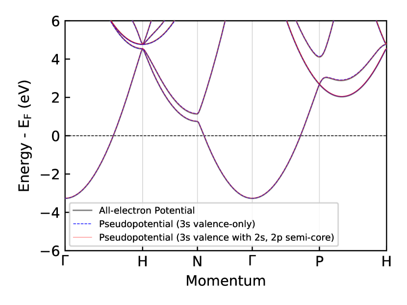
Figure 1: Comparison of the DFT energy dispersion for bcc Na within the local density approximation (LDA) using experimental equilibrium unit-cell volume, calculated using the full-potential all-electron electronic structure method with RSPt (grey) and the pseudopotential method with Quantum Espresso. Two atomic pseudopotentials are used, with (red) and without (blue) the semi-core 2$s$ state. The energy levels are plotted relative to the Fermi level, $E_{F}$. These calculations use the same convergence parameters as in Fig. 2.

For a pseudopotential to have general applicability, it is important that it is transferable [28, 29] to different chemical environments, e.g., works for a molecule, or a material that forms covalent or ionic bonds, under ambient or high pressure, or even for a crystal surface. The transferability of a pseudopotential characterizes the accuracy with which the pseudopotential reproduces the effect of the all-electron potential in different chemical environments. One way to test for the transferability of a pseudopotential to a different chemical environment is by comparing the calculated Kohn-Sham energy eigenvalues with the self-consistent all-electron results [28]. This raises the question of whether one can apply the normal protocols for generating pseudopotentials, but instead of using the atomic state as reference electronic configuration take an environment that more closely resembles the native conditions where the pseudopotential is supposed to be used, be it in a solid or molecular state. We will refer to the standard pseudopotentials derived using the free isolated atom as the reference configuration as an atomic pseudopotential. In this work, we also use the solid state as a reference configuration. We refer to such pseudopotentials as in-situ pseudopotentals, and will demonstrate as a proof-of-concept in this paper that these pseudopotentials can reproduce all-electron results to very high accuracy.

The advantage of an in-situ pseudopotental is that it is tailored to the specific chemical environment of the material (e.g. under high compression) and, as a result, it can in general be used as an expedient, accurate and computationally inexpensive tool to analyze electronic structures of complex systems, e.g. as discussed in Ref [30]. In addition, the use of the solid-state environment to generate in-situ pseudopotentials is motivated by the fact that the scattering properties of a pseudopotential constructed for an isolated atom might be different from those of the same atom placed in a material. This is particularly of concern, when the environment in the solid is drastically different from that of an atom, e.g., when neighboring atoms in an ionic bonded material cause large charge transfer effects that affect the multiple scattering properties. Similarly, it can be troublesome to use an atomic generated pseudopotential evaluated at ambient conditions, for a solid state calculation of the electronic structure of a material under extreme compression.

In this paper, we outline the critical steps to generate in-situ pseudopotentials, and calculate for bcc Na the band dispersion using an in-situ pseudopotential generated from an all-electron reference state obtained from the full-potential linear muffin-tin orbitals method (RSPt software [6]). This result is then compared with the band structure obtained from two different atomic (i.e., generated from an atomic reference state), scalar-relativistic and norm-conserving pseudopotentials using the Quantum Espresso software [31]. The main difference is that the first atomic pseudopotential (i) contains only the valence 3$s$ state of Na (i.e., valence-only) while the second (ii) contains not only the valence 3$s$ state, but also the $2s$ and $2p$ semi-core states. The former [32] pseudopotential is a Troullier-Martins [33] pseudopotential generated using FHI98PP [34] and includes nonlinear core correction [35]. It has only one Kleinman-Bylander-Vanderbilt [20, 25] projector per angular channel. The latter pseudopotential is an optimized norm-conserving Vanderbilt pseudopotential (ONCVPSP) [36] obtained from the PseudoDojo project [37]. It does not use nonlinear core correction and has two projectors per angular channel. All pseudopotential calculation with Qunatum Espresso uses a kinetic-energy cutoff of 100 Ry for the plane wave basis expansion, a $\mathbf{k}$-grid of $24\times 24\times 24$ and LDA [38] for the self-consistent DFT calculation.

  Method

Simply described, the method to generate in-situ pseudopotentials can be divided into three distinct steps. (1) Calculate the eigenstates of the Kohn-Sham equations of the solid using an all-electron method. (2) Construct the pseudowavefunction by modifying the corresponding valence state to remove any nodes in the core region while exactly preserving the wavefunction in the interstitial region. (3) Generate a pseudopotential that gives rise to this pseudowavefunction. We begin by describing step (3) in Sec. 2.1 before moving on to the more technical details of step (2) in Sec. 2.2.

The inverse pseudopotential problem

For the purpose of this section, we first assume that the pseudowavefunction, $\tilde{\Psi}_{\mathbf{k}n}$, and its energy eigenvalue, $\tilde{\epsilon}_{\mathbf{k}n}$, for each $\mathbf{k}$ point in the Brillouin zone and band $n$, are already known. Next, consider the eigenvalue equation

$$H_{pp}\tilde{\Psi}_{\mathbf{k}n}= \tilde{\epsilon}_{\mathbf{k}n}\tilde{\Psi}_{\mathbf{k}n},$$ (1)

where $\mathbf{k}$ is crystal momentum restricted to the first Brillouin zone, $n$ is a band index for the given $\mathbf{k}$, and

$$H_{pp}= -\nabla^{2}+V_{pp}(\mathbf{r})$$ (2)

$$= -\nabla^{2}+\sum_{\mathbf{G}}V_{\mathbf{G}}e^{i\mathbf{G}\cdot\mathbf{r}},$$ (3)

$$\tilde{\Psi}_{\mathbf{k}n}(\mathbf{r})= \sum_{\mathbf{G}}\tilde{\mathcal{D}}_{\mathbf{G}}^{\mathbf{k}n}e^{i(\mathbf{G}+\mathbf{k})\cdot\mathbf{r}}.$$ (4)

Here, $\mathbf{G}$ runs over the reciprocal lattice vectors, and $V_{\mathbf{G}}$ and $\tilde{\mathcal{D}}_{\mathbf{G}}^{\mathbf{k}n}$ are, respectively, the plane wave expansion coefficients for the pseudopotential $V_{pp}$ and pseudowavefunction, $\tilde{\Psi}_{\mathbf{k}n}$. The $\tilde{\Psi}_{\mathbf{k}n}$ is known as the pseudowavefunction as it is the solution of a Hamiltonian involving a pseudopotential. In Eqs.  2 and 3, we have used Rydberg atomic units. Multiplying Eq. 1 by $e^{-i(\mathbf{G^{\prime}+k})\cdot\mathbf{r}}$ and integrating over $\mathbf{r}$, we obtain the expression,

$${\left(\mathbf{G}+\mathbf{k}\right)^{2}}\tilde{\mathcal{D}}_{\mathbf{G}}^{\mathbf{k}n}+\sum_{\mathbf{G}^{\prime}}V_{\mathbf{G}^{\prime}}\tilde{\mathcal{D}}_{\mathbf{G}-\mathbf{G}^{\prime}}^{\mathbf{k}n}= \;\tilde{\epsilon}_{\mathbf{k}n}\tilde{\mathcal{D}}_{\mathbf{G}}^{\mathbf{k}n}.$$ (5)

In practice, the sum over $\mathbf{G^{\prime}}$ in the plane wave expansion of the pseudopotential and pseudowavefunction is truncated for a finite number ($N$), of coefficients. Therefore, for a given eigenstate, Eq. 5 corresponds to $N$ linear equations with $N$ unknowns, which in matrix form can be written as (note that $\mathbf{k}$ and $n$ are state labels, not matrix indices)

$$\mathbf{M}^{\mathbf{k}n}\mathbf{v}=\mathbf{u}^{\mathbf{k}n},$$ (6)

where

$$\left[\mathbf{v}\right]_{\mathbf{G}}= \;V_{\mathbf{G}},$$ (7)

$$\left[\mathbf{u}^{\mathbf{k}n}\right]_{\mathbf{G}}= \left(\tilde{\epsilon}_{\mathbf{k}n}-{(\mathbf{G}+\mathbf{k})^{2}}\right)\tilde{\mathcal{D}}_{\mathbf{G}}^{\mathbf{k}n},$$ (8)

$$\left[\mathbf{M}^{\mathbf{k}n}\right]_{\mathbf{G},\mathbf{G}^{\prime}}= \;\tilde{\mathcal{D}}_{\mathbf{G}-\mathbf{G}^{\prime}}^{\mathbf{k}n}.$$ (9)

The matrix $\mathbf{M}^{\mathbf{k}n}$ is a blocked Toeplitz matrix. The linear system of equations in Eq. 6 can therefore be solved by a blocked Levinson algorithm, which formally produce the pseudopotential

$$\mathbf{v}= \left(\mathbf{M}^{\mathbf{k}n}\right)^{-1}\mathbf{u}^{\mathbf{k}n}.$$ (10)

While this pseudopotential is only constructed to exactly reproduce the eigenvalue $\tilde{\epsilon}_{\mathbf{k}n}$ for a particular $\mathbf{k}$, we will see in Sec. 3 that the procedure gives a pseudopotential that gives satisfactory results for eigenvalues throughout the Brillouin zone, i.e. also for eigenvalues calculated at $\mathbf{k}^{\prime}\neq\mathbf{k}$.

Choice of wavefunction and practical implementation

While the method described in Sec. 2.1 is straightforward, the difficulty lies in generating an appropriate wavefunction $\tilde{\Psi}_{\mathbf{k}n}$ to use as input. In principle one can calculate it by first solving an all-electron electronic structure problem, thereby obtaining the true energy eigenvalue and wavefunction. Hence, by finding a solution to

$$H_{AE}{\Psi}_{\mathbf{k}n}(\mathbf{r})= {\epsilon}_{\mathbf{k}n}{\Psi}_{\mathbf{k}n}(\mathbf{r}),$$ (11)

where $H_{AE}$ is the all-electron Hamiltonian, one could in principle solve Eqs. 7 - 10, by setting $\tilde{\Psi}_{\mathbf{k}n}$ equal to the true all-electron wavefunction, ${\Psi}_{\mathbf{k}n}$, and by identifying $\tilde{\epsilon}_{\mathbf{k}n}$ with ${\epsilon_{\mathbf{k}n}}$. In this way one is guaranteed that the pseudopotential that comes out of Eq. 10 gives the same eigenvalue and wavefunction as the all-electron Hamiltonian. A pseudopotential generated at one particular $\mathbf{k}$-point, e.g. the $\Gamma$-point, can then be used in Eqs. 1 - 3, to calculate eigenvalues and eigenstates throughout the Brillouin zone. One can also envision using this pseudopotential for other, but similar, conditions, e.g. a crystal at compressed volumes compared to the condition where the pseudopotential is originally calculated from. In this approach, the valence states generated by an all-electron calculation are expected to have nodes in the core region, which will require a very large number of the basis vectors to converge the calculation if the plane wave basis set is used (Eq. 4). A solution to this problem is to replace the fast oscillating part of ${\Psi}_{\mathbf{k}n}$, that is primarily close to an atomic nucleus, with a smooth pseudowavefunction, $\tilde{\Psi}_{\mathbf{k}n}$, that is nodeless, while still keeping $\tilde{\epsilon}_{\mathbf{k}n}={\epsilon_{\mathbf{k}n}}$. This is the usual way of pseudopotential theory, albeit we propose here to do it using its native solid state as the reference electronic configuration, and not the free atom.

The description that follows aims at describing how a smooth, nodeless pseudowavefunction can be evaluated from an all-electron wavefunction that is obtained from a full-potential linear muffin-tin orbitals method, as implemented in the RSPt package [6]. We start with the general approach of writing the all-electron wavefunction as a linear combination of known basis functions, namely, the linear muffin-tin orbitals (LMTOs),

$${\Psi}_{\mathbf{k}n}(\mathbf{r})=\sum_{\Lambda}{\mathcal{C}}_{\Lambda}^{\mathbf{k}n}\phi_{\Lambda}^{\mathbf{k}}(\mathbf{r}),$$ (12)

where $\phi_{\Lambda}^{\mathbf{k}}$ are the LMTOs introduced by Andersen [4], where the $\Lambda$ index groups many indices, such as the tail energy of the basis function, angular momenta and type of atomic species. We emphasize that $\mathbf{k}n$ are state labels, not indices. The LMTOs are defined with respect to two regions: the muffin-tin and the interstitial regions. In the latter, the LMTO basis function is either a Hankel or a Neumann function, depending on choice of kinetic energy of this basis function. For practical reasons, in the RSPt package [6], the wavefunction in the interstitial region is calculated as an exact Fourier series. This is done by extending a Hankel or Neumann function from the interstitial region into the muffin-tin sphere with an analytic smooth function, for fast converged Fourier series expansion. This means that the interstitial basis function is defined over all space, and matrix elements of e.g. the Hamiltonian or the Bloch wavefunction overlap is truncated inside the muffin-tins using a step function.

Following Ref. [6], we define a pseudo basis function, $\tilde{\phi}_{\Lambda}^{\mathbf{k}}$, as the Fourier-transformed Hankel or Neumann function, that in the interstitial region is identical to the all-electron LMTO basis function:

$$\tilde{\phi}_{\Lambda}^{\mathbf{k}}(\mathbf{r})=\sum_{\mathbf{G}}\tilde{A}_{\Lambda\mathbf{G}}^{\mathbf{k}}e^{i(\mathbf{G}+\mathbf{k})\cdot\mathbf{r}},$$ (13)

where $\tilde{A}_{\Lambda\mathbf{G}}^{\mathbf{k}}$ are the Fourier coefficients of this basis function. This function can now be used for the expression of the Fourier series in Eqs. 1 - 4, that should be defined over all space, i.e. including the muffin-tin region. We start by considering the all-electron wavefunction, in Eq. 11, that in the interstitial can also be expressed in terms of the Fourier series, in Eq. 13. This can be done by replacing $\phi_{\Lambda}^{\mathbf{k}n}$ in Eq. 12 with $\tilde{\phi}_{\Lambda}^{\mathbf{k}n}$. By construction, this replacement does not influence the wavefunction in the interstitial region. However, it drastically modifies the wavefunction in the muffin-tin region, since the part of the muffin-tin orbital that is defined in the muffin-tin sphere, where in general the radial component has many nodes, is replaced by a smooth function. For this reason we distinguish the true wavefunction, Eq. 12, from a pseudowavefunction,

$$\tilde{\Psi}_{\mathbf{k}n}(\mathbf{r})=\sum_{\Lambda}{\mathcal{C}}_{\Lambda}^{\mathbf{k}n}\tilde{\phi}_{\Lambda}^{\mathbf{k}}(\mathbf{r}).$$ (14)

Notice that the expansion coefficients in Eqs. 12 and 14, ${\mathcal{C}}_{\Lambda}^{\mathbf{k}n}$, should be the same. Writing out explicitly the form of $\tilde{\phi}_{\Lambda}^{\mathbf{k}n}$ we can express the pseudowavefunction as

$$\tilde{\Psi}_{\mathbf{k}n}(\mathbf{r})=\sum_{\Lambda}{\mathcal{C}}_{\Lambda}^{\mathbf{k}n}\sum_{\mathbf{G}}\tilde{\mathcal{A}}_{\Lambda\mathbf{G}}^{\mathbf{k}}e^{i(\mathbf{G}+\mathbf{k})\cdot\mathbf{r}}.$$ (15)

Using this equation, the coefficients $\tilde{\mathcal{D}}$ of Eq. 4 will be given by

$$\tilde{\mathcal{D}}^{\mathbf{k}n}=\sum_{\Lambda}{\mathcal{C}}_{\Lambda}^{\mathbf{k}n}\tilde{\mathcal{A}}_{\Lambda\mathbf{G}}^{\mathbf{k}}.$$ (16)

The form given by the latter equation should be used in the pseudowavefunction given in Eq. 4 to calculate the corresponding pseudopotential, by following Eqs. 6 - 10. A practical way to evaluate a pseudopotential with this method is to first perform a normal all-electron calculation to obtain ${\mathcal{C}}_{\Lambda}^{\mathbf{k}n}$ coefficients (and the eigenvalue, $\epsilon_{\mathbf{k}n}$). In this process, the Fourier coefficients of the pseudo-basis function are kept (from Eqs. 13 and 16), which enables an evaluation of Eq. 4. The so-obtained pseudowavefunction and eigenvalue are used in Eqs. 6 - 10, to obtain the required pseudopotential.

Although the description above seems straight forward, we note that these modifications are done in the full-potential method of Ref. [6], independently of whether a pseudopotential is to be extracted or not. They are in line with the aims of the pseudopotential approach, but are strictly speaking related to the computational benefits associated with having fewer coefficients in the Fourier expansion. To be useful for a pseudopotential approach, we also need to ensure that low-lying ‘ghost states’ do not appear. To understand the ‘ghost state’ problem, consider applying Eq. 10 immediately to the unmodified valence state. By construction, the resulting pseudopotential gives rise to a Hamiltonian that contains this eigenstate. However, the full Hilbert space also contains smoother states and these tend to have lower energy. This is not surprising since states with lower energy do exist in the original problem, namely the core states. The purpose of the pseudopotential approach is to generate an effective Hamiltonian for which the valence states are the low energy states and it is therefore essential to remove radial nodes in the wavefunction. While the procedure outlined above does reduce the number of radial nodes, it is not constructed to guarantee an absence of nodes. It also does not guarantee norm conservation. In this work, we are focused on constructing norm-conserving pseudopotentials (even though this constraint of norm-conservation can be relaxed in future works, similar to that in the ultrasoft-pseudopotential [20, 21] and PAW methods [22, 23], at the expense of a more complex mathematical representation, versus the simpler representation of norm-conserving pseudopotentials [39, 33]).

For these reasons we modify the pseudowavefunction further to make it nodeless and ensure norm conservation. It is the aggregate of these modifications to the pseudowavefunction that are compensated for through the pseudopotential. Only by modifying the wavefunction in the core region is it possible to preserve the chemical properties that emerge from the pseudopotential, since chemical bonding is mainly determined by the wavefunction overlap in the interstitial region between atoms. The expression we arrived at for the nodeless, normalized pseudowavefunction is

$$\hat{\Psi}_{\mathbf{k}n}(r,\theta,\varphi)=c(r)\tilde{\Psi}_{\mathbf{k}n}(r,\theta,\varphi)+N(1-c(\mathbf{r}))f(r,\theta,\varphi),$$ (17)

where $f(r,\theta,\phi)$ is a smooth function with the same angular dependence as $\tilde{\Psi}_{\mathbf{k}n}(r,\theta,\varphi)$ and $c(\mathbf{r})$ smoothly interpolates between $\tilde{\Psi}^{\mathbf{k}n}(r,\theta,\varphi)$ in the interstitial region and $f(r,\theta,\varphi)$ in the muffin-tin region. For convenience, we have also factored out a constant $N$ from $f(r,\theta,\varphi)$ that will be used to ensure that the pseudowavefunction is normalized. Note that Eq. 17 is general, in sense that it can be applied to an all-electron valence state, although we for technical reasons apply it to the pseudowavefunction obtained from Eq. 16, $\tilde{\Psi}^{\mathbf{k}n}$ .

In this manuscript we provide a proof-of-principle demonstration of the method for the energy dispersion of the Na $3s$-band. Adapted for this state we choose

$$c(r)= \left\{\begin{array}[]{cc}0&|r|<R_{0},\\ 1&|r|>R_{1},\\ \left.3x^{2}-2x^{3}\right|_{x=\frac{r-R_{0}}{R_{1}-R_{0}}}&\textrm{otherwise}.\\ \end{array}\right.$$ (21)

The node-free, normalized pseudowavefunction is then defined, with a suitable choice of $f(r,\theta,\phi)$ in Eq. 17. We return to appropriate choices of this function below. First we remark that in Eq. 21, $R_{0}$ and $R_{1}$ are chosen so as to obtain a smooth interpolation without nodes. In general, $R_{0}$ should be larger than the radius of the outermost radial node, and we have $R_{0}<R_{1}<R_{MT}$, where $R_{MT}$ is the muffin-tin radius. Returning now to the choice of $f(r,\theta,\phi)$, we have in the numerical examples presented below focused on the valence state of Na, which is dominated by the $3s$ state. This function has no angular component and it is sufficient to use $f(r,\theta,\phi)=f(r)$. We have made two choices for $f(r)$; a constant value of 1 and a polynomial of degree 15. In the latter choice, we determined the expansion coefficients through a least square fit of a pseudowavefunction obtained from a Quantum Espresso calculation using the valence-only pseudopotential (this is shown as a green line in Fig. 2a). Below we will compare the results for both choices of $f(r)$.

The constant, $N$, in Eq. 17 is determined by requiring that $\hat{\Psi}_{\mathbf{k}n}$ is normalized to 1,

This is solved by,

$$N= -\frac{B}{C}\pm\frac{\sqrt{\left(1-A\right)B+C^{2}}}{B},$$ (23)

where,

$$A= \langle c\tilde{\Psi}_{\mathbf{k}n}|c\tilde{\Psi}_{\mathbf{k}n}\rangle,$$ (24)

$$B= \langle(1-c)f|(1-c)f\rangle,$$ (25)

$$C= \textrm{Re}\left(\langle c\tilde{\Psi}_{\mathbf{k}n}|(1-c)f\rangle\right).$$ (26)

  Results

In Fig. 2, we compare the radial components of $\hat{\Psi}_{\mathbf{k}n}(r,\theta,\varphi)$ and $\tilde{\Psi}_{\mathbf{k}n}(r,\theta,\varphi)$ for the lowest eigenvalue of bcc Na, obtained at the $\Gamma$ point. Note that we show in the figure results of pseudowavefunction and band dispersion for two choices of $f(r)$ in Eq. 17: a constant and a 15-degree polynomial. Included for reference is also a pseudowavefunction obtained from a Quantum Espresso calculation (from which one choice of $f(r)$ was obtained). In this calculation, we set the muffin-tin radius, $R_{MT}=3.285$ a.u., which is approximately 95% of the touching radius between two nearest Na atoms, and use $R_{0}=0.55R_{MT}$ and $R_{1}=0.75R_{MT}$ for the constant $f(r)$ and $R_{0}=0.75R_{MT}$ and $R_{1}=0.9R_{MT}$ for the polynomial. The all-electron calculation that is used to evaluate the pseudowavefunction uses the local density approximation (LDA) [40, 41]. As LMTO basis vectors, we use three 3$s$ orbitals, three 3$p$ orbitals and two 3$d$-orbitals in the muffin-tin spheres. In the interstitial region, the tails have kinetic energies of 0.3 Ry (for 3$s$-, 3$p$- and 3$d$-orbitals), -2.3 Ry (for 3$s$-, 3$p$- and 3$d$-orbitals) and -1.5 Ry (for 3$s$- and 3$p$-orbitals). The number of $\mathbf{k}$-points used to converge the results were $12\times 12\times 12$. As in Fig. 1, the experimental [27] lattice parameter of 4.225 Å was used.

It is clear from Fig. 2 (a and c) that $\hat{\Psi}_{\mathbf{k}n}(r,\theta,\varphi)$ and $\tilde{\Psi}_{\mathbf{k}n}(r,\theta,\varphi)$ are identical in the interstitial region. These wavefunctions also coincide with the full, true all-electron wavefunction in the interstitial region (data not shown). From a detailed inspection of the radial components of $\hat{\Psi}_{\mathbf{k}n}(r,\theta,\varphi)$ and $\tilde{\Psi}_{\mathbf{k}n}(r,\theta,\varphi)$ we note that the latter has a single node, as opposed to the two nodes expected from a 3$s$ state. The single node of the otherwise rather soft behavior of $\tilde{\Psi}_{\mathbf{k}n}(r,\theta,\varphi)$, has to do with how the full-potential method of Ref. [6] represents the basis functions in the interstitial, in particular as a Fourier series (see Eqs. 6.38 - 6.42 of Ref. [6]). In order to obtain a pseudopotential that is as smooth as possible from Eqs. 6 - 10, we have made use of $\hat{\Psi}_{\mathbf{k}n}(r,\theta,\varphi)$ (in a Fourier representation) instead of $\tilde{\Psi}_{\mathbf{k}n}(r,\theta,\varphi)$, since the former pseudowavefunction is by construction node-less inside the muffin-tin sphere (see Fig. 2a). This choice leads to a much smoother pseudowavefunction, that may be expressed with a minimum number of Fourier components. For this reason we have used the Fourier representation of $\hat{\Psi}_{\mathbf{k}n}(r,\theta,\varphi)$ in all the steps outlined in Eqs. 1 - 10, discussed in Sec. 2.

In Fig. 2 (a and c), we note that depending on choice of $f(r)$, the behaviour of $\hat{\Psi}_{\mathbf{k}n}(r,\theta,\varphi)$ inside the muffin-tin region is different. For the choice of a 15-degree polynomial for $f(r)$, $\hat{\Psi}_{\mathbf{k}n}(r,\theta,\varphi)$ is by construction similar to the function obtained from a calculation based on Quatum Espresso (see Fig. 2a). Although the behavior in the core region is explicitly constructed, a good match is not guaranteed from the outset. The freedom provided through the normalization constant $N$, and the fact that the two regions (interstitial and muffin-tin) are stitched together with the help of the interpolation function $c(r)$ rather than being matched at the muffin-tin boundary, means the two functions are allowed to differ. The near-perfect match in spite of this is a reassurance of the soundness of the interpolation procedure.

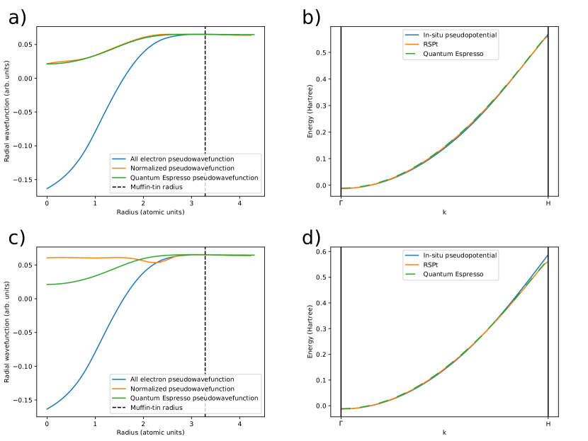
Figure 2: (a and c) Calculated radial component of the pseudowavefunction $\tilde{\Psi}_{\mathbf{k}n}(r,\theta,\varphi)$ (blue, for definition see text), calculated radial part of the modified pseudowavefunction $\hat{\Psi}_{\mathbf{k}n}(r,\theta,\varphi)$ (orange, for definition see text), and radial pseudowavefunction calculated with Quantum Espresso using a valence-only atomic pseudopotential (green). (b and d) Calculated energy dispersion of the valence band states of bcc Na along the $\Gamma-H$ high symmetry direction of the first Brillouin zone. Three types of methods are used to calculate the energy bands: the all-electron full potential method (orange), the in-situ pseudopotential method as described of this paper (blue) and the pseudopotential method using a valence-only atomic pseudopotential (green). Panels (a) and (b) show results for the choice of $f(r)$ being a polynomial of degree 15 that is least-square fitted to the radial pseudowavefunction calculated with Quantum Espresso using a valence-only pseudopotential (using $R_{0}=0.75R_{MT}$ and $R_{1}=0.9R_{MT}$). Panels (c) and (d) show results for a choice of $f(r)=1$ (using $R_{0}=0.55R_{MT}$, and $R_{1}=0.75R_{MT}$. The muffin-tin radius, $R_{MT}=3.285$ Å, is denoted using dashed lines in all panels). In all these calculations, a $11\times 11\times 11$ mesh is used for the Fourier expansion of the pseudopotential.

After having calculated a pseudopotential, using Eqs. 1 - 10 in combination with $\hat{\Psi}_{\mathbf{k}n}(r,\theta,\varphi)$, we calculate eigenvalues and eigenvectors from Eq. 5. This represents therefore the solution to a local pseudopotential, and the calculation was done using 1331 plane-wave components in the expansion of the wavefunction. In Fig. 2 (b and d) we show the resulting energy dispersion along the high-symmetry line, $\Gamma-H$, of the first Brillouin zone, for two different in-situ pseudopotentials, one from a choice of $f(r)$ as a constant and one from a choice of $f(r)$ being a 15-degree polynomial. The two different in-situ pseudopotential results are compared to the energy dispersion of an all-electron full-potential electronic structure method (see Fig. 2 b and d) . We first note that the whole methodology described above is designed to yield the same eigenvalue and wavefunction in the interstitial region at the $\Gamma$ point. Hence, it is gratifying that for the $\Gamma$ point the eigenvalues from the in-situ pseudopotential method and the all-electron full-potential method differ only in the sixth significant digit, irrespective of choice of $f(r)$ in Eq. 21. Furthermore, the energy dispersion is seen to agree very well between in-situ pseudopotential theory and all-electron theory throughout the Brillouin zone. When comparing the two in-situ pseudopotentials (evaluated from constant and polynomial choice of $f(r)$), we note that the agreement in band dispersion between all-electron theory and any in-situ pseudopotential theory is surprisingly good. This holds true even when we set $f(r)=1$. The latter has a pseudowavefunction that in the core region differs significantly from a traditional behaviour (e.g. as seen from the results obtained from the Quantum Espresso calculation). The poorer choice of $f(r)=1$ nevertheless results in an in-situ pseudopotential that reproduces all-electron results throughout most of the Brillouin zone, demonstrating the robustness of our approach. The largest difference for the eigenvalues is observed at the zone boundary, which is not unexpected, considering that these states have crystal momentum farthest away from that state where the in-situ pseudopotential was calculated (the $\Gamma$ point).

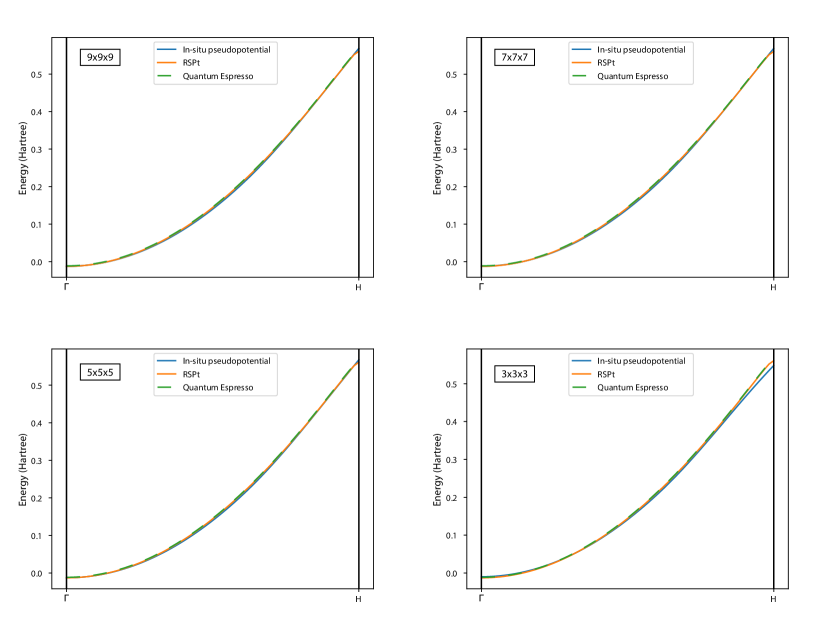
Figure 3: Calculated energy dispersion of the valence band states of bcc Na, along the $\Gamma-H$ high symmetry direction of the first Brillouin zone. It is similar to the plot in Panel (b) of Fig. 2, except that the Fourier expansion of the psuedopotential is truncated to a smaller $N\times N\times N$ mesh as specified in the inset of each panel. As in Panel (b) of Fig. 2, three types of methods are used to calculate the energy bands: the all-electron full potential method (orange), the in-situ pseudopotential method as described of this paper (blue) and the pseudopotential method using a valence-only atomic pseudopotential (green). Here, $f(r)$ is the 15-degree polynomial least-square fitted to the radial pseudowavefunction calculated with Quantum Espresso using a valence-only pseudopotential (using $R_{0}=0.75R_{MT}$ and $R_{1}=0.9R_{MT}$)

As a final point, we also investigate the effect of truncating the Fourier coefficients of the in-situ pseudopotential, to gauge its smoothness. In Fig. 3 we show results of energy bands of bcc Na, when the in-situ pseudopotential, being calculated from Eq.10, has its higher Fourier components truncated. In practice this means keeping from the original in-situ pseudopotential, only components from a $N\times N\times N$ mesh (that is smaller than the origial mesh of $11\times 11\times 11$). It is interesting to note from Fig. 3 that good agreement between full-potential, all-electron theory and in-situ pseudopotential theory can be is achieved for all considered Fourier meshes, except the very smallest one ($3\times 3\times 3$). This indicates that equal accuracy to all-electron theory can be achieved from an in-situ pseudopotential theory, that is represented by only 125 ($5\times 5\times 5$) plane waves.

  Discussion and Conclusion

In this paper, we have demonstrated a proof-of-concept of how it is possible to calculate a pseudopotential from an all-electron, electronic structure method. For reference, in Fig. 2 c, d we also consider for a much cruder choice of core function, using $f(r)=1$, $R_{0}=0.55R_{MT}$ and $R_{1}=0.75R_{MT}$. The agreement of the eigenvalues is in fact surprisingly good also in this case, even though the pseudowavefunction differs significantly from that of the Quantum Espresso in the core region. Technically, this amounts to solving the inverse Kohn-Sham equation for one or a few eigenvalues and eigenstates, which have been obtained from the all-electron theory. The method proposed here relies on replacing the rapidly oscillating part of an eigenstate close to the nucleus (in the muffin-tin sphere) with a smoother and much softer form, which allows for fast convergence in the expansion of the Fourier series. In principle, this method is not restricted to using the solid state as the reference electronic configuration and can be readily extended to molecular species or crystal surfaces. It also does not require the use of LMTOs as basis functions and is, for example, also suitable for the LAPW or LCAO basis set. It is also not mandatory to use the zone center to evaluate the in-situ pseudopotential, other points of the Brillouin zone can be used, and it is possible to take averages of in-situ pseudopotentials from several points, to get a final in-situ pseudopotential to use for further studies.

In this work, we limit our discussion to the construction of the local components of the pseudopotentials. Its extension to the nonlocal components [19, 25, 20] is natural, and necessary in order to resolve higher lying energy bands, an effort which represents ongoing work. Even without the nonlocal components, the proposed in-situ pseudopotential method reproduces energy dispersion of the 3$s$-like band states to good accuracy throughout the Brillouin zone. The largest discrepancy between the in-situ pseudopotential outlined here, and results from an all-electron method, is at the Brillouin zone boundary. This is expected since these zone-boundary states have an admixture of angular momentum characters that can only be properly described with the inclusion of the nonlocal components in the in-situ pseudopotential. Furthermore, the crystal momentum of these states is the farthest away from the k-point at which the in-situ pseudopotential was calculated.

It is well-known that the transferability of an atomic pseudopotential can be systematically improved, by reducing $r_{c}$ at the cost of greater computational cost [19]. With the construction of the pseudopotential in situ, using the native state as the reference, this requirement of transferability can potentially be relaxed if an in-situ pseudopotential is used. This may even allow for a larger pseudopotential radii cutoff for the same convergence, thereby reducing the number of Fourier components needed in the series expansion and a reduced computational cost. This method also automatically takes into account the nonlinear [35] nature of the exchange and correlation interaction between the core and valence charge densities, which is important when a valence-only pseudopotential is used for an akali metal like Na [35], which only has one electron in the valence shell. In a typical calculation using atomic pseudopotentials, these interactions are first assumed to be linear, before adding the nonlinear core contributions as a perturbative correction. Another benefit of generating the pseudopotential in the native solid-state environment is that basis-set convergence is already controlled at the level of the all-electron calculation. For example, if the LMTO-basis set is used for the all-electron calculation (as in our case), convergence parameters will include the number of Fourier-components to match LMTOs, as well as core-leakage that will indicate if certain semi-core states have to be treated as valence states. Computational cost versus accuracy can then be optimized.

The methodology suggested here can also be extended to include the spin-polarized case. One must then keep track of spin-indices of the all-electron generated eigenvalues and eigenvectors in the analysis presented in Sec. 2. Following the steps in the methods section that describe the pseudopotential generation, one could then obtain in-situ pseudopotentials for spin-up states and spin-down states separately. After unscreening of these pseudopotentials (removing contributions from exchange and correlation of the electron gas, as well as the Hartree potential) one would obtain spin-dependent pseudopotentials that are able to accurately reproduce magnetic moments and spin-dependent information of all-electron theory. Spin-orbit effects may also be incorporated in the proposed in-situ pseudopotentials, since the method outlined can be used for any spin-orbit calculated eigenstate. Finally, we speculate that the in-situ pseudopotential can be generalized, such that effects from a self-energy, $\Sigma^{\mathbf{k}}$, (e.g., obtained from the $GW$ approximation or the dynamical mean field theory) are incorporated in the pseudopotential. This could be achieved by associating $\tilde{\epsilon}_{\mathbf{k}n}$ with $\tilde{\epsilon}_{\mathbf{k}n}+Re\Sigma_{\mathbf{k}}$ in Eq. 1. The steps outlined above represent an investigation that is underway.

References

- [1] Bloch, F. Über die quantenmechanik der elektronen in kristallgittern. Zeitschrift für physik 52, 555–600 (1929).
- [2] Korringa, J. On the calculation of the energy of a bloch wave in a metal. Physica 13, 392–400 (1947).
- [3] Kohn, W. & Rostoker, N. Solution of the schrödinger equation in periodic lattices with an application to metallic lithium. Phys. Rev. 94, 1111–1120 (1954). URL https://link.aps.org/doi/10.1103/PhysRev.94.1111.
- [4] Andersen, O. K. Linear methods in band theory. Phys. Rev. B 12, 3060–3083 (1975). URL https://link.aps.org/doi/10.1103/PhysRevB.12.3060.
- [5] Skriver, H. & Skriver, H. The LMTO Method: Muffin-tin Orbitals and Electronic Structure. Lecture Notes in Computer Science (Springer-Verlag, 1984).
- [6] Wills, J. M. et al. Full-Potential Electronic Structure Method, vol. 167 of Springer Series in Solid-State Sciences (Springer Berlin Heidelberg, Berlin, Heidelberg, 2010). URL http://link.springer.com/10.1007/978-3-642-15144-6.
- [7] Heine, V. The pseudopotential concept. vol. 24 of Solid State Physics, 1 – 36 (Academic Press, 1970). URL http://www.sciencedirect.com/science/article/pii/S0081194708600697.
- [8] Cohen, M. L. & Heine, V. The fitting of pseudopotentials to experimental data and their subsequent application. vol. 24 of Solid State Physics, 37 – 248 (Academic Press, 1970). URL http://www.sciencedirect.com/science/article/pii/S0081194708600703.
- [9] Cohen, M. L. & Chelikowsky, J. R. Electronic Structure and Optical Properties of Semiconductors, vol. 75 of Springer Series in Solid-State Sciences (Springer Berlin Heidelberg, Berlin, Heidelberg, 1988). URL http://link.springer.com/10.1007/978-3-642-97080-1.
- [10] Payne, M. C., Teter, M. P., Allan, D. C., Arias, T. & Joannopoulos, a. J. Iterative minimization techniques for ab initio total-energy calculations: molecular dynamics and conjugate gradients. Reviews of modern physics 64, 1045 (1992).
- [11] Chelikowsky, J. Electrons in Semiconductors: Empirical and ab initio Pseudopotential Theories, 1–41 (2011).
- [12] Fermi, E. E. fermi. Nuovo cimento 11, 157 (1934).
- [13] Hellmann, H. A new approximation method in the problem of many electrons. The Journal of Chemical Physics 3, 61–61 (1935). URL https://doi.org/10.1063/1.1749559. https://doi.org/10.1063/1.1749559.
- [14] Antončík, E. A new formulation of the method of nearly free electrons. Cechoslovackij fiziceskij zurnal 4, 439–451 (1954).
- [15] Antončík, E. Approximate formulation of the orthogonalized plane-wave method. Journal of Physics and Chemistry of Solids 10, 314 – 320 (1959). URL http://www.sciencedirect.com/science/article/pii/0022369759900071.
- [16] Phillips, J. C. & Kleinman, L. New method for calculating wave functions in crystals and molecules. Physical Review 116, 287 (1959).
- [17] Kleinman, L. & Phillips, J. C. Crystal potential and energy bands of semiconductors. iii. self-consistent calculations for silicon. Phys. Rev. 118, 1153–1167 (1960). URL https://link.aps.org/doi/10.1103/PhysRev.118.1153.
- [18] Hamann, D. R., Schlüter, M. & Chiang, C. Norm-conserving pseudopotentials. Phys. Rev. Lett. 43, 1494–1497 (1979). URL https://link.aps.org/doi/10.1103/PhysRevLett.43.1494.
- [19] Bachelet, G. B., Hamann, D. R. & Schlüter, M. Pseudopotentials that work: From h to pu. Phys. Rev. B 26, 4199–4228 (1982). URL https://link.aps.org/doi/10.1103/PhysRevB.26.4199.
- [20] Vanderbilt, D. Soft self-consistent pseudopotentials in a generalized eigenvalue formalism. Phys. Rev. B 41, 7892–7895 (1990). URL https://link.aps.org/doi/10.1103/PhysRevB.41.7892.
- [21] Blöchl, P. E. Generalized separable potentials for electronic-structure calculations. Phys. Rev. B 41, 5414–5416 (1990). URL https://link.aps.org/doi/10.1103/PhysRevB.41.5414.
- [22] Blöchl, P. E. Projector augmented-wave method. Phys. Rev. B 50, 17953–17979 (1994). URL https://link.aps.org/doi/10.1103/PhysRevB.50.17953.
- [23] Kresse, G. & Joubert, D. From ultrasoft pseudopotentials to the projector augmented-wave method. Phys. Rev. B 59, 1758–1775 (1999). URL https://link.aps.org/doi/10.1103/PhysRevB.59.1758.
- [24] Schwerdtfeger, P. The pseudopotential approximation in electronic structure theory. ChemPhysChem 12, 3143–3155 (2011).
- [25] Kleinman, L. & Bylander, D. M. Efficacious form for model pseudopotentials. Phys. Rev. Lett. 48, 1425–1428 (1982). URL https://link.aps.org/doi/10.1103/PhysRevLett.48.1425.
- [26] Lejaeghere, K. et al. Reproducibility in density functional theory calculations of solids. Science 351 (2016). URL https://science.sciencemag.org/content/351/6280/aad3000. https://science.sciencemag.org/content/351/6280/aad3000.full.pdf.
- [27] Barrett, C. S. X-ray study of the alkali metals at low temperatures. Acta Crystallographica 9, 671–677 (1956). URL //scripts.iucr.org/cgi-bin/paper?a01768.
- [28] Goedecker, S. & Maschke, K. Transferability of pseudopotentials. Physical Review A 45, 88–93 (1992).
- [29] Filippetti, A., Vanderbilt, D., Zhong, W., Cai, Y. & Bachelet, G. B. Chemical hardness, linear response, and pseudopotential transferability. Physical Review B 52, 11793–11804 (1995). 9505002.
- [30] Sarma, D. D. et al. The electronic structure of NiAl and NiSi. Journal of Physics: Condensed Matter 1, 9131–9139 (1989). URL https://doi.org/10.1088/0953-8984/1/46/007.
- [31] Giannozzi, P. et al. Quantum ESPRESSO: a modular and open-source software project for quantum simulations of materials. Journal of Physics: Condensed Matter 21, 395502 (2009). 0906.2569.
- [32] Our Na pseudopotential is downloaded from https://www.abinit.org/sites/default/files/PrevAtomicData/psp-links/lda_fhi.html and converted to UPF format. It is also available at https://www.quantum-espresso.org/upf_files/Na.pw-mt_fhi.UPF . Accessed: 2021-01-30.
- [33] Troullier, N. & Martins, J. L. Efficient pseudopotentials for plane-wave calculations. Physical review B 43, 1993 (1991).
- [34] Fuchs, M. & Scheffler, M. Ab initio pseudopotentials for electronic structure calculations of poly-atomic systems using density-functional theory. Computer Physics Communications 119, 67–98 (1999). 9807418.
- [35] Louie, S. G., Froyen, S. & Cohen, M. L. Nonlinear ionic pseudopotentials in spin-density-functional calculations. Phys. Rev. B 26, 1738–1742 (1982). URL https://link.aps.org/doi/10.1103/Louie1982.
- [36] Hamann, D. R. Optimized norm-conserving vanderbilt pseudopotentials. Phys. Rev. B 88, 085117 (2013). URL https://link.aps.org/doi/10.1103/PhysRevB.88.085117.
- [37] van Setten, M. et al. The pseudodojo: Training and grading a 85 element optimized norm-conserving pseudopotential table. Computer Physics Communications 226, 39 – 54 (2018). URL http://www.sciencedirect.com/science/article/pii/S0010465518300250. Our Na pseudopotential is downloaded from "http://www.pseudo-dojo.org/pseudos/nc-sr-04_pw_standard/Na.upf.gz". Accessed: 2021-01-30.
- [38] Perdew, J. P. & Wang, Y. Accurate and simple analytic representation of the electron-gas correlation energy. Phys. Rev. B 45, 13244–13249 (1992). URL https://link.aps.org/doi/10.1103/PhysRevB.45.13244.
- [39] Hamann, D. R. Generalized norm-conserving pseudopotentials. Phys. Rev. B 40, 2980–2987 (1989). URL https://link.aps.org/doi/10.1103/PhysRevB.40.2980.
- [40] Hedin, L. & Lundqvist, B. I. Explicit local exchange-correlation potentials. Journal of Physics C: Solid State Physics 4, 2064–2083 (1971). URL https://doi.org/10.1088/0022-3719/4/14/022.
- [41] von Barth, U. & Hedin, L. A local exchange-correlation potential for the spin polarized case. i. Journal of Physics C: Solid State Physics 5, 1629–1642 (1972). URL https://doi.org/10.1088/0022-3719/5/13/012.