Absolute 3D Pose Estimation and Length Measurement of Severely Deformed Fish from Monocular Videos in Longline Fishing

Abstract

Monocular absolute 3D fish pose estimation allows for efficient fish length measurement in the longline fisheries, where fishes are under severe deformation during the catching process. This task is challenging since it requires locating absolute 3D fish keypoints based on a short monocular video clip. Unlike related works, which either require expensive 3D ground-truth data and/or multiple-view images to provide depth information, or are limited to rigid objects, we propose a novel frame-based method to estimate the absolute 3D fish pose and fish length from a single-view 2D segmentation mask. We first introduce a relative 3D fish template. By minimizing an objective function, our method systematically estimates the relative 3D pose of the target fish and fish 2D keypoints in the image. Finally, with a closed-form solution, the relative 3D fish pose can help locate absolute 3D keypoints, resulting in the frame-based absolute fish length measurement, which is further refined based on the statistical temporal inference for the optimal fish length measurement from the video clip. Our experiments show that this method can accurately estimate the absolute 3D fish pose and further measure the absolute length, even outperforming the state-of-the-art multi-view method.

Index Terms—  3D pose, Fish length, Longline fishing

1 Introduction

Given one single image of a deformed fish such as Pacific Halibut during longline fishing [1], our goal is to design a pipeline that receives as input the whole single-view image and produces as outputs the absolute 3D keypoints location and length of the fish [2] .

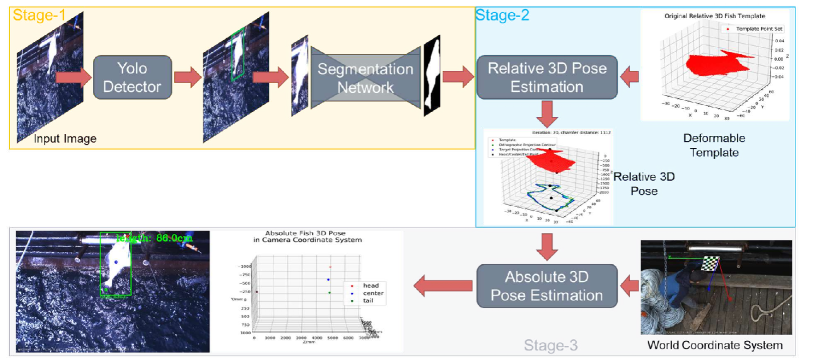
As shown in Fig.2, in Stage-1, we use the YOLO object detector [3] and an encoder-decoder FCN architecture for instance segmentation [4], refined by histogram back projection [5]. We have ground truth labels to train both models.

Our main contributions are in the last two stages. Stage-2 introduces a relative 3D fish template and chamfer distance loss [6]. Only relying on the target’s 2D segmentation mask from Stage-1, Stage-2 is able to estimate the relative 3D pose of the target and three 2D keypoints in image. Stage-3 introduces a novel 3D localization method to locate these keypoints in absolute 3D space and measure the length of the fish.

(a)

(b)

Fig. 1: 3D Template: (a) A binary mask of a standard flat Pacific Halibut; (b) The initial original 3D point set of foreground pixels is the relative 3D fish template on $Z=0$ plane.

Fig. 2: Pipeline: Note that in the world coordinate system, the red axis is $Z$ axis. In the left bottom corner, camera image plane is on $Z=0$ plane, and $Z$ axis is depth, with unit being millimeter. So, the above fish is about 5 meters away from the camera.

2 Proposed Method

2.1 Relative 3D Fish Template

Inspired by [7, 8], we introduce a relative 3D fish template, whose unit is a pixel. It is a 3D point set on a surface generated from a Pacific Halibut Template, as illustrated in Fig.1. The origin point is the center point of the fish body. We denote the initial template point set as $S_{0}=\{(x_{0i},y_{0i},z_{0i})\in R^{3}\}_{i=1}^{N}$, where $N$ is the total number, and $0$ represents the initial point set before any deformable transformation. To simulate the deformable pose of the fish, the template iteratively executes the following four transformation sequentially:

Scale Transformation We denote the scale parameter as $s\in R$. The scaling transformation is to multiply $s$ with each point, $(x_{0i},y_{0i},z_{0i})$, in the template point set $S_{0}$:

$$\left(x_{1i},y_{1i},z_{1i}\right)=s\cdot\left(x_{0i},y_{0i},z_{0i}\right),$$ (1)

resulting in a new point set $S_{1}=\{(x_{1i},y_{1i},z_{1i})\in R^{3}\}_{i=1}^{N}$.

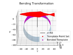
Bending Transformation We denote the bending parameter as $r\in R$ being the radius of a cylinder, which is tangent with the template at the initial position, as illustrated in Fig.1. The bending transformation maps each point, $(x_{1i},y_{1i},z_{1i})$, in $S_{1}$ to a new 3D point, $(x_{2i},y_{2i},z_{2i})\in R^{3}$, on the cylinder:

$$\begin{cases}x_{2i}&=x_{1i},\\ z_{2i}&=r\left(1-\cos\frac{y_{1i}}{r}\right),\\ y_{2i}&=\frac{z_{2i}}{\tan\frac{y_{1i}}{2r}},\\ \end{cases}$$ (2)

which is fish length preserving, resulting in a new point set, $S_{2}=\{(x_{2i},y_{2i},z_{2i})\in R^{3}\}_{i=1}^{N}$ (the purple surface in Fig.1).

Translation Transformation We denote the translation parameters as $(T_{x},T_{y},0)\in R^{3}$:

$$\left(x_{3i},y_{3i},z_{3i}\right)=\left(x_{2i},y_{2i},z_{2i}\right)+\left(T_{x},T_{y},0\right),$$ (3)

resulting in a new point set $S_{3}=\{(x_{3i},y_{3i},z_{3i})\in R^{3}\}_{i=1}^{N}$.

Rotation Transformation We denote three rotation parameters as $\alpha,\beta,\gamma\in[0,2\pi]$, which respectively represent the rotation degree around $x$, $y$, $z$ axis [9]. We construct three basic (elemental) rotation matrices, $R(\gamma)$, $R(\beta)$, and $R(\alpha)\in R^{3\times 3}$ and rotation transform each point, $(x_{3i},y_{3i},z_{3i})$ to a new point $(x_{4i},y_{4i},z_{4i})\in R^{3}$:

$$\left(x_{4i},y_{4i},z_{4i}\right)=\left(x_{3i},y_{3i},z_{3i}\right)\cdot R(\gamma)\cdot R(\beta)\cdot R(\alpha).$$ (4)

Finally, after performing these four transformations one-by-one iteratively, we denote the final relative 3D template as $S_{4}=\{(x_{4i},y_{4i},z_{4i})\}_{i=1}^{N}\in R^{3}$. These four transformations are differentiable with respect to their parameters, which enables us to do relative 3D pose estimation in the next section.

(a)

(b)

(c)

(d)

(e)

Fig. 3: Relative 3D Pose Estimation: (a) A target mask from Stage-1; (b) After applying a Canny edge detector on (a), indicated by the blue point set in (c); (c) Black dots are predefined head/center/tail keypoints, yellow connections and cyan connections respectively are the first term and second term in chamfer distance. Those connections are ‘forces’ to pull the template contour close to the target contour, a similar concept with ’intrinsic/extrinsic forces’ in [10]; (d) A middle shot; (e) The final shot.

2.2 Relative 3D Pose Estimation

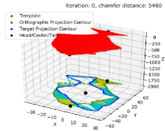
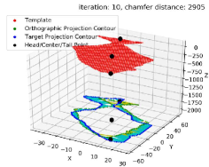
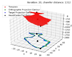
Based on a target’s 2D mask, we can directly estimate the relative 3D pose of the target fish and 2D keypoints in image without using expensive 3D ground truth [11, 12] or multi-view images. We iteratively minimize the chamfer distance between the orthographic projection contour of 3D template and one target’s 2D mask contour, as illustrated in Fig.3.

Orthographic Projection Contour We get the orthographic projection points of the 3D template by directly setting each point, $(x_{4i},y_{4i},z_{4i})$ to $(x_{4i},y_{4i},0)$. Then, we convert these points into a binary mask and execute Canny edge detector [13] and denote the orthographic projection contour points as, $S_{template}=\{(x_{4i},y_{4i},z_{4i})\in R^{3}\}_{i}^{n}\in S_{4}$, where $n$ varies given different transformations’ parameters.

Target Contour The target contour points are acquired by applying the Canny edge detector on the target’s 2D binary mask from Stage-1. Because the template’s center point is at the origin point before four transformations, we also transform the mask image center to the origin point and then get the final target contour point set, denoted as $S_{target}=\{(x_{j},y_{j},z_{j})\in R^{3}\}_{j=1}^{m}$.

Chamfer Distance Loss Given a fixed $S_{target}$, and an adjustable $S_{template}$, we iteratively and sequentially adjust each point in $S_{template}$ with seven parameters in four deformation transformations so that the chamfer distance, Eq. 5, is minimized by gradient descent [14]:

$$d_{CD}\left(S_{template},S_{target}\right)=\sum_{p_{i}\in S_{template}}\min_{q_{j}\in S_{target}}\|p_{i}-q_{j}\|_{2}^{2}$$ (5)

$$+\sum_{q_{j}\in S_{target}}\min_{p_{i}\in S_{template}}\|p_{i}-q_{j}\|_{2}^{2},$$

where the first term implies, for each point $p_{i}=(x_{4i},y_{4i},z_{4i})\in S_{template}$, calculate the Euclidean distance of this point and its nearest point $q_{j}=(x_{j},y_{j},z_{j})\in S_{target}$. The second term implies, for each point in $q_{j}=(x_{j},y_{j},z_{j})\in S_{target}$, find the nearest point $p_{i}=(x_{4i},y_{4i},z_{4i})\in S_{template}$ to calculate their Euclidean distance. After optimization, the relative 3D fish template’s pose is the estimated target’s relative 3D pose in the camera coordinate system but with $pixel$ as a unit. Plus, since we can predefine three keypoints (head, center and tail) on the template, their orthographic projections are the 2D keypoints in the target mask, as illustrated in Fig.3, denoted as $h_{2d}$ $(U_{h},V_{h})$, $c_{2d}$ $(U_{c},V_{c})$, $t_{2d}$ $(U_{t},V_{t})$ respectively in the whole image coordinate system. We denote center, head, and tail points in target’s relative 3D pose as $h$ $(x_{h},y_{h},z_{h})$, $c$ $(x_{c},y_{c},z_{c})$, and $t$ $(x_{t},y_{t},z_{t})$ respectively.

2.3 Absolute 3D Localization

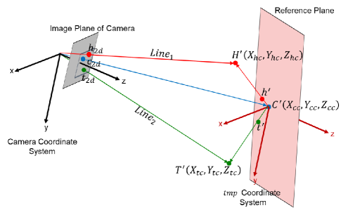
To have a 3D length measurement of the fish body, we introduce an absolute 3D localization method to locate three keypoints in absolute 3D, denoted respectively as $H^{\prime}$ $(X_{hc},Y_{hc},Z_{hc})$, $C^{\prime}$ $(X_{cc},Y_{cc},Z_{cc})$, and $T^{\prime}$ $(X_{tc},Y_{tc},Z_{tc})$, where the second subscript $c$ means the camera coordinate system and the unit is $millimeter$ instead of $pixel$. This task is formulated as the following closed-form solution.

Back Projection We first use camera intrinsic parameters to back project $h_{2d}$ $(U_{h},V_{h})$, $c_{2d}$ $(U_{c},V_{c})$, $t_{2d}$ $(U_{t},V_{t})$ to 3D space in the camera coordinate system without depth:

$$\left[\begin{array}[]{c}X\\ Y\\ 1\end{array}\right]=K^{-1}\left[\begin{array}[]{c}U\\ V\\ 1\end{array}\right],$$ (6)

where $K$ denotes camera intrinsic parameters, that is a $3\times 3$ matrix, obtained by method from [15]. Now for $h_{2d}$, $c_{2d}$, $t_{2d}$, respectively we get $h^{\prime\prime}$ $(X_{h},Y_{h},1)$, $c^{\prime\prime}$ $(X_{c},Y_{c},1)$, and $t^{\prime\prime}$ $(X_{t},Y_{t},1)$ in the camera coordinate system.

Reference Plane In the longline fishing [16, 17], all fish are hooked and pulled up by a line. So our assumption is that all fish’s center points are always on a reference plane, which coincides with the plane of checkerboard of known grid size used in the camera calibration, defined as $Z=0$ plane in the world coordinate system, as illustrated in the right bottom corner of Fig.2. Then we use the solvePnP method [18] to calculate the rotation matrix, $R_{3\times 3}$, and translation vector, $T_{3\times 1}$, between the world coordinate system and the camera coordinate system. Under our assumption, center point $C^{\prime}$ is a point $(X_{cw},Y_{cw},0)$ in the world coordinate system. With $R_{3\times 3},\ T_{3\times 1}$ and $K_{3\times 3}$, we can get $Z_{cc}$ (depth) with Eq.7. We also need to calculate homography matrix $H$ between the image plane and $Z=0$ plane in the world coordinate system:

$$\begin{cases}H\quad=\quad K_{3\times 3}&\cdot\left[\begin{array}[]{lll}R_{1}&R_{2}&T\end{array}\right]_{3\times 3},\\ \left[\begin{array}[]{c}X_{cw}/Z_{cc}\\ Y_{cw}/Z_{cc}\\ 1/Z_{cc}\end{array}\right]&=H^{-1}\cdot\left[\begin{array}[]{c}U_{c}\\ V_{c}\\ 1\end{array}\right],\end{cases}$$ (7)

where $R_{1},\ R_{2}$ are the first two columns in $R_{3\times 3}$.

Finally, with $Z_{cc}$ (depth), we can get the center point $C^{\prime}$:

$$(X_{cc},Y_{cc},Z_{cc})=Z_{cc}\cdot(X_{c},Y_{c},1).$$ (8)

3D Localization A 3D localization method with a closed-form solution is introduced to calculate head point $H^{\prime}$ and tail point $T^{\prime}$, which are on the following two lines respectively:

$$Line_{1}:(X,Y,Z) =m\cdot(X_{h},Y_{h},1),m\in R,$$ (9)

$$Line_{2}:(X,Y,Z) =n\cdot(X_{t},Y_{t},1),n\in R.$$

As illustrated in Fig.4, we set up a new coordinate system with unit being $pixel$, called $tmp$, whose origin point is at $C^{\prime}$ and has no relative rotation with respect to the camera coordinate system but the translation vector between them is $(X_{cc},Y_{cc},Z_{cc})$. In Section 2.2, we got the relative 3D pose, i.e., $h$, $c$, and $t$ in the camera coordinate system with unit being $pixel$. Now we want to estimate the absolute fish pose centered at $C^{\prime}$ so we translate $h$, $c$ and $t$ to the $tmp$ coordinate system by translating $c$ to $tmp$’s origin point:

$$c^{\prime} =(X_{cc},Y_{cc},Z_{cc}),$$ (10)

$$h^{\prime} =(x_{h}-x_{c},y_{h}-y_{c},z_{h}-z_{c})+(X_{cc},Y_{cc},Z_{cc}),$$

$$t^{\prime} =(x_{t}-x_{c},y_{t}-y_{c},z_{t}-z_{c})+(X_{cc},Y_{cc},Z_{cc}),$$

where $t^{\prime}$ $(x_{tc},y_{tc},z_{tc})$ and $h^{\prime}$ $(x_{hc},y_{hc},z_{hc})$ are relative head point and tail point in the camera coordinate system. Note that the absolute head point, $H^{\prime}$, and tail point, $T^{\prime}$, must also lie on the following lines $C^{\prime}h^{\prime}$ and $C^{\prime}t^{\prime}$ respectively:

$$(X,Y,Z) =a\cdot(x_{hc},y_{hc},z_{hc})+(1-a)\cdot(X_{cc},Y_{cc},Z_{cc}),a\in R,$$ (11)

$$(X,Y,Z) =b\cdot(x_{tc},y_{tc},z_{tc})+(1-b)\cdot(X_{cc},Y_{cc},Z_{cc}),b\in R.$$

So, $H^{\prime}$ must be the intersection point of line $C^{\prime}h^{\prime}$ and $Line_{1}$, and $T^{\prime}$ must be the intersection point of line $C^{\prime}t^{\prime}$ and $Line_{2}$. To find $H^{\prime}$ and $T^{\prime}$, we minimize the distance between two lines, which results in a closed-form solution with the simple least-squares method [19], omitted due to the pages limit. Finally, and the absolute fish length can thus be calculated:

$${Length} ={\mid H^{\prime}T^{\prime}\mid}\cdot{\frac{\overset{\frown}{ht}}{\mid ht\mid}},$$ (12)

where $\frac{\overset{\frown}{ht}}{\mid ht\mid}$ is the bending ratio. The left bottom corner of Fig.2 is a 3D localization example.

Fig. 4: 3D Localization: $h^{\prime}$, $C^{\prime}$, and $t^{\prime}$ define the relative 3D pose. $H^{\prime}$, $C^{\prime}$, and $T^{\prime}$ defines the absolute 3D pose.

3 Experiments

Due to the complexity of collecting data during longline fishing, we have 738 ground-truth labeled fish lengths measurement histogram and the corresponding several hours’ stereo videos under different weather conditions and view angles. We can only use the difference between predicted length histogram and ground truth length histogram to evaluate all competing methods. Specifically, we use bias, root mean square deviation (RMSD), Kullback-Leibler (KL) divergence [20], and earth mover’s distance (EMD) [21] to access the performance. For all frames of the same fish in one short video clip, we estimate its length in each frame and use a Gaussian distribution to remove outliers beyond $2\cdot\sigma$ and take average of the rest predicted lengths.

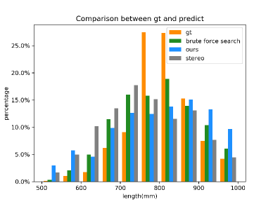
Comparison with the state-of-the-art Compared with [16], which requires stereo image pairs as input and is more difficult to deploy in the challenging at-sea environment while ours only needs a single-view image. Fig.5 and Table.1 show superior performance of our method in all four metrics.

Fig. 5: Results: Only check lengths in $[500,1000]mm$ because most lengths are within this range. $y$ axis is percentage of fish number in bins over total number. $x$ axis is length bins.

Table 1: Comparison Evaluation and Ablation Study

Method	Bias(mm)	EMD(mm)	RMSD	KL
Stereo [16]	-40.5	46.0	7.9%	0.26
BFS	-10.2	24.2	5.6%	0.11
BFS w/o Bending	-55.4	60.0	7.9%	0.28
Ours w/o Bending	-95.4	99.3	10.4%	0.53
Ours	-9.3	43.1	7.3%	0.23

Ablation Study To replace our optimization part, we construct a database consisting of thousands of orthographic projection images of relative 3D fish template under various deformation parameters. Given a 2D mask of a target, we brute-force search (BFS) to find one projection image with maximum intersection of union with this 2D mask and use its deformation parameters to generate the relative 3D pose for Stage-3. Fig.5 and Table.1 show our optimization has favorable performance as BFS but BFS is more time consuming and memory demanding. Besides, we remove bending ratio and test BFS method and ours. Table.1 shows bending modeling is critical in fish length measurement.

4 Conclusions

We proposed a relative deformable 3D fish template, a chamfer distance based optimization method to predict relative 3D pose from a 2D instance mask, and a 3D localization method with a closed-form solution to estimate absolute 3D fish pose. Our experiments show that our monocular method outperforms the state-of-the-art stereo method, our optimization method has favorable performance as brute-force search and our bending modeling is critical in fish length measurement.

References

- [1] Jie Mei, Jenq-Neng Hwang, Suzanne Romain, Craig Rose, Braden Moore, and Kelsey Magrane, “Video-based hierarchical species classification for longline fishing monitoring,” 2021.
- [2] Tsung-Wei Huang, Jenq-Neng Hwang, and Craig S Rose, “Chute based automated fish length measurement and water drop detection,” in 2016 IEEE International Conference on Acoustics, Speech and Signal Processing (ICASSP). IEEE, 2016, pp. 1906–1910.
- [3] Joseph Redmon, Santosh Divvala, Ross Girshick, and Ali Farhadi, “You only look once: Unified, real-time object detection,” in Proceedings of the IEEE conference on computer vision and pattern recognition, 2016, pp. 779–788.
- [4] Olaf Ronneberger, Philipp Fischer, and Thomas Brox, “U-net: Convolutional networks for biomedical image segmentation,” in International Conference on Medical image computing and computer-assisted intervention. Springer, 2015, pp. 234–241.
- [5] Meng-Che Chuang, Jenq-Neng Hwang, Kresimir Williams, and Richard Towler, “Automatic fish segmentation via double local thresholding for trawl-based underwater camera systems,” in 2011 18th IEEE International Conference on Image Processing. IEEE, 2011, pp. 3145–3148.
- [6] Haoqiang Fan, Hao Su, and Leonidas J. Guibas, “A point set generation network for 3d object reconstruction from a single image,” CoRR, vol. abs/1612.00603, 2016.
- [7] Gaoang Wang, Jenq-Neng Hwang, Farron Wallace, and Craig Rose, “Multi-scale fish segmentation refinement and missing shape recovery,” IEEE Access, vol. 7, pp. 52836–52845, 2019.
- [8] Sanja Fidler, Sven Dickinson, and Raquel Urtasun, “3d object detection and viewpoint estimation with a deformable 3d cuboid model,” in Advances in Neural Information Processing Systems 25, F. Pereira, C. J. C. Burges, L. Bottou, and K. Q. Weinberger, Eds., pp. 611–619. Curran Associates, Inc., 2012.
- [9] James Arvo, “Fast random rotation matrices,” in Graphics Gems III (IBM Version), pp. 117–120. Elsevier, 1992.
- [10] Demetri Terzopoulos, Andrew Witkin, and Michael Kass, “Constraints on deformable models: Recovering 3d shape and nonrigid motion,” Artificial intelligence, vol. 36, no. 1, pp. 91–123, 1988.
- [11] Nanyang Wang, Yinda Zhang, Zhuwen Li, Yanwei Fu, Wei Liu, and Yu-Gang Jiang, “Pixel2mesh: Generating 3d mesh models from single rgb images,” in Proceedings of the European Conference on Computer Vision (ECCV), 2018, pp. 52–67.
- [12] Edward J. Smith, Scott Fujimoto, Adriana Romero, and David Meger, “Geometrics: Exploiting geometric structure for graph-encoded objects,” CoRR, vol. abs/1901.11461, 2019.
- [13] J. Canny, “A computational approach to edge detection,” IEEE Transactions on Pattern Analysis and Machine Intelligence, vol. PAMI-8, no. 6, pp. 679–698, 1986.
- [14] Sebastian Ruder, “An overview of gradient descent optimization algorithms,” CoRR, vol. abs/1609.04747, 2016.
- [15] Z. Zhang, “A flexible new technique for camera calibration,” IEEE Transactions on Pattern Analysis and Machine Intelligence, vol. 22, no. 11, pp. 1330–1334, 2000.
- [16] Tsung-Wei Huang, Jenq-Neng Hwang, Suzanne Romain, and Farron Wallace, “Fish tracking and segmentation from stereo videos on the wild sea surface for electronic monitoring of rail fishing,” IEEE Transactions on Circuits and Systems for Video Technology, vol. 29, no. 10, pp. 3146–3158, 2018.
- [17] Kresimir Williams, Nathan Lauffenburger, Meng-Che Chuang, Jenq-Neng Hwang, and Rick Towler, “Automated measurements of fish within a trawl using stereo images from a camera-trawl device (camtrawl),” Methods in Oceanography, vol. 17, pp. 138–152, 2016.
- [18] Xiao-Shan Gao, Xiao-Rong Hou, Jianliang Tang, and Hang-Fei Cheng, “Complete solution classification for the perspective-three-point problem,” IEEE Transactions on Pattern Analysis and Machine Intelligence, vol. 25, no. 8, pp. 930–943, 2003.
- [19] Abraham Charnes, Edward L Frome, and Po-Lung Yu, “The equivalence of generalized least squares and maximum likelihood estimates in the exponential family,” Journal of the American Statistical Association, vol. 71, no. 353, pp. 169–171, 1976.
- [20] Solomon Kullback and Richard A Leibler, “On information and sufficiency,” The annals of mathematical statistics, vol. 22, no. 1, pp. 79–86, 1951.
- [21] Elizaveta Levina and Peter Bickel, “The earth mover’s distance is the mallows distance: Some insights from statistics,” 02 2001, vol. 2, pp. 251 – 256 vol.2.