Statistically Profiling Biases in Natural Language Reasoning Datasets and Models

Abstract

Recent work has indicated that many natural language understanding and reasoning datasets contain statistical cues that may be taken advantaged of by NLP models whose capability may thus be grossly overestimated. To discover the potential weakness in the models, some human-designed stress tests have been proposed but they are expensive to create and do not generalize to arbitrary models. We propose a light-weight and general statistical profiling framework, ICQ (I-See-Cue), which automatically identifies possible biases in any multiple-choice NLU datasets without the need to create any additional test cases, and further evaluates through blackbox testing the extent to which models may exploit these biases.

1 Introduction

Deep neural models have shown to be effective in a large variety of natural language inference (NLI) tasks Bowman et al. (2015); Wang et al. (2018); Mostafazadeh et al. (2016); Roemmele et al. (2011); Zellers et al. (2018). Many of these tasks are discriminative by nature, such as predicting a class label or an outcome given a textual context, as shown in the following example:

Example 1.

Natural language inference in SNLI dataset, with ground truth bolded.

Premise: A swimmer playing in the surf watches a low flying airplane headed inland.

Hypothesis: Someone is swimming in the sea.

Label: a) Entailment. b) Contradiction. c) Neutral.

The number of candidate labels may vary. Humans solve such questions by reasoning the logical connections between the premise and the hypothesis, but previous work Naik et al. (2018); Schuster et al. (2019) has found that some NLP models can solve the questions fairly well by looking only at the hypothesis (or “conclusion” in some work) in the datasets. It is widely speculated that this is because in many datasets, the hypotheses are manually crafted and may contain artifacts that would be predictive of the correct answer. Such “hypothesis-only” tests can identify problematic questions in the dataset if the question can be answered correctly without the premise. While such a method to evaluate the quality of a dataset is theoretically sound, it i) usually relies on training a heavy-weight model such as Bert, which is costly to evaluate, ii) does not provide explanation why the question is a culprit, and iii) cannot be used to evaluate a model since a model that can make a correct prediction using only the hypothesis is not necessarily a bad model: it is just not given the complete data.

Inspired by black-box testings in software engineering, CheckList Jurafsky et al. (2020) assesses the weakness of models without the need to know the details of the model. It does so by providing additional stress test cases according to predefined linguistic features. Unfortunately, to ensure the correctness of these additional cases, the templates must be carefully crafted with substantial restrictions, thus limiting the testing space and complicating the implementation. Furthermore, with CheckList, you only get to know what the model is incapable of doing but won’t know what the model has learned from the data.

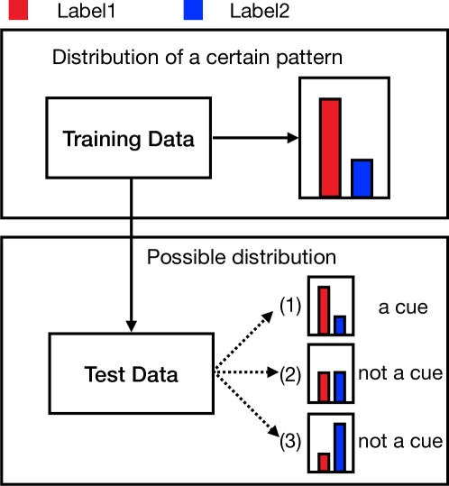
Figure 1: Example of a cue.

In this paper, our view is that the existing test sets for these tasks are not sufficiently exploited. Why do we go the extra mile to generate new test cases which are potentially incorrect, when we can test the models using existing test sets but from different perspectives? With this objective in mind, we propose ICQ (“I-see-cue”), an open-source evaluation framework  for evaluating both the dataset and the corresponding models. In this framework, one test dataset can be seen as multiple test sets from different perspectives.

Previous studies Gururangan et al. (2018); Sanchez et al. (2018); Poliak et al. (2018) showed that statistical bias on linguistic features (e.g., sentiment, repetitive words and even shallow n-grams) which have statistical correlation with specific labels in benchmark datasets can be predictive of the correct answer. We call such biases artificial spurious cues when they appear both in the training and test datasets with a similar distribution over the prediction values. We illustrate this in Figure 1. Once these cues are neutralized from the test data, previously successful models may degrade substantially on it, suggesting that the model has taken advantage of the biased feature and is hence not as robust as assumed against with such cues.

In summary, this paper makes the following contributions:

• we provide a light-weight but effective method to uncover the statistical biases and cues in NL reasoning datasets;

• we propose two simple tests to quantitatively and visually assess whether a given model has taken advantage of a spurious cue when making predictions;

• we evaluate the statisical bias issues comprehensively on 10 popular NLR datasets and 4 models and not only reaffirm some of the findings from previous work but also discover some new perspectives in these datasets and models;

• we created an online demonstration system to showcase the results and invite users to evaluate their own datasets and models.

2 Preliminary Definition

We define an instance $x$ of a natural language reasoning (NLR) task dataset $X$ as

$$x=(p,h,l)\in X,$$ (1)

where $p$ is the context against which to do the reasoning ($p$ corresponds to “premise” in Example 1); $h$ is the hypothesis given the context $p$; $l\in\mathcal{L}$ is the label that depicts the type of relation between $p$ and $h$. The size of the relation set $\mathcal{L}$ varies with tasks.

There is another type of natural language reasoning tasks which are also in the form of multiple-choice questions, but their choices are a fixed set of labels, as shown below.

Example 2.

A story in ROCStory dataset, with ground truth bolded Mostafazadeh et al. (2016).

Context: Rick grew up in a troubled household. He never found good support in family, and turned to gangs. It was n’t long before Rick got shot in a robbery. The incident caused him to turn a new leaf.

Ending 1: He joined a gang.

Ending 2: He is happy now.

We can transform the this case into two separate problem instances, still in the same form as in Eq. (1), $u_{1}=(context,ending1,false)$ and $u_{2}=(context,ending2,true)$, where $L={true,false}$.

3 Approach

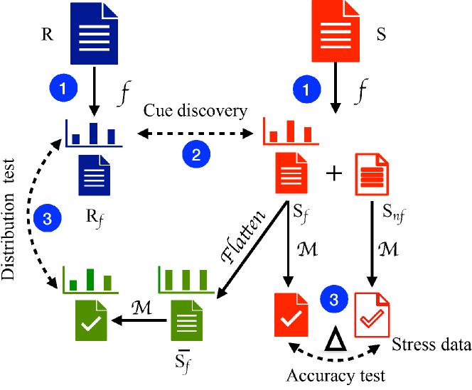
Figure 2: ICQ Workflow. ①: data filtering phase; ②: cue discovery phase; ③: model probing phase.

The ICQ framework is illustrated in Figure 2. In data filtering phase, it extracts from the dataset those problem instances that contain a given linguistic feature $f$. In cue discovery phase, it identifies the possible cues in this dataset. Finally, in model probing phase, it does two tests: “accuracy test” and “distribution test”. Next we will discuss these phases in more details.

3.1 Linguistic Features

In this work, we consider the following linguistic features: Word (unigram tokens in the input sentences), Typos, NER (named entity recognition), Tense (temporal order of events), Negation, Sentiment, and Overlap (words occurring both in the premise and the hypothesis). The above list is by no means exhaustive, but just a starting point for users who can come up with additional features that are relevant to their task or domain.

3.1.1 Word

For a dataset $X$, we collect a set of all words $V$ that ever exist in $X$. A word feature is defined as the existence of a word $w\in V$ either in the premise or the hypothesis. Because $V$ is generally very large, in practice, we may narrow it down to words that sufficiently popular in $X$. That is, we may remove words that seldom appear in $X$.

3.1.2 Sentiment

For each data instance $x$, we can compute its sentiment value as:

$$S(x)=\text{sgn}(\sum_{w\in x}polar(w)),$$ (2)

where $polar(w)$ is the sentiment polarity (-1, 0, or 1) of $w$ determined by a look-up from a pretrained sentiment lexicon . We say $x$ has a positive/negative/neutral sentiment feature if $S(x)$ = 1, -1 or 0, respectively.

3.1.3 Tense

We say that an instance $x$ has past, present or future tense feature if $x$ carries one of these tenses, respectively, by the POS tag of the root verb in $p$ or $h$.

3.1.4 Negation

Previous work has observed that negative words (“no”, “not” or “never”) may be indicative of a certain label in NLI tasks for some models. The existence of a negation feature in $x$ is decided by dependency parsing .

3.1.5 Overlap

In many models, substantial word-overlap between the premise and the hypothesis sentences causes incorrect inference, even if they are unrelated McCoy et al. (2019). We define that an overlap feature exists in $x$ if there’s at least one word (except for stop words) that occurs both in $p$ and $h$.

3.1.6 NER

We define the NER feature as the existence of either PER, ORG, LOC, TIME, CARDINAL entity in $x$. We use the NLTK ner toolkit for this purpose.

3.1.7 Typos

We say an instance $x$ has typo feature if there exists at least one typo in $x$. We use a pretrained spelling model  to detect all typos in a sentence. We don’t distinguish the types of mispellings here.

As we mentioned in Example 2, multiple choice questions are each split into two data instances with opposite labels (T or F), and the premises in these two instances are identical. Therefore, it is not useful to detect features within the premises alone. Consequently, for MCQ type of datasets, all the above features except for Overlap are only applied on the hypotheses.

3.2 Discovering Cues in Dataset

Once we have defined the linguistic features, we can build a data filter for each feature values. A filter takes a dataset and returns a subset of instances associated with that feature value. For example, there is a filter for the word “like”; there is a filter for “PER” entity; and there is filter for “negative” sentiment, etc.

For each feature $f$, we apply its filter to both the training data and test data of $X$, denoted as $R$ and $S$ in Figure 2, resulting in $R_{f}$ and $S_{f}$. Only those features that appear both in the training and test data are qualified as possible cues for a dataset. Let $y_{i}$ be the number of instances with label $l_{i}$ in the filtered dataset, then we can compute the bias of the label distribution for a filtered set as the mean squared error (MSE):

$$mse(Y)=\frac{1}{|L|}\sum_{i}(y_{i}-\hat{y_{i}})^{2}$$ (3)

where $\hat{y_{i}}$ is the mean of $y_{i}$. The larger $mse(Y)$, the more “pointed” the label distribution and more biased. Furthermore, if the filtered training set and the filtered test set are biased similarly, the Jensen-Shannon Divergence Lin (1991) between them is small:

$$jsd(R_{f},S_{f})=\frac{1}{2}\left(R_{f}\parallel M\right)+\frac{1}{2}\left(S_{f}\parallel M\right),$$ (4)

where $M=\frac{1}{2}\left(R_{f}+S_{f}\right)$. Finally, we define a cueness score as

$$cue(f,X)=\frac{mse(R_{f})}{\exp(jsd(R_{f}),S_{f}))}$$ (5)

which represents how much a dataset $X$ is biased against a feature $f$.

3.3 Probing Bias in Model

Suppose we already know that a dataset $X$ is infected with a cue $f$ from previous test in Section 3.2. However, just because the dataset is infected with a cue doesn’t mean the model trained from this dataset necessarily exploits that cue. Here we propose a simple method to probe any model instance trained from the given biased dataset  to see if it actually takes advantage of that cue $f$ and by how much.

We can do that through two simple tests: accuracy test and distribution test. In accuracy test, we simply assess the prediction accuracies of the model $M$ on the filtered test set and on the remaining test data, and call them $acc(S_{f})$ and $acc(S_{nf})$, respectively. The accuracy test says that if the difference between these two accuracies, i.e, $\Delta=acc(S_{f})-acc(S_{nf})$ is greater 0, then the model is considered to be biased and to have exploited this cue. The value of $\Delta$ measures the extent of the bias.

Distribution test is a visual test. We first create a “stress data set” $\overline{S_{f}}$ by “flattening” the label distribution in $S_{f}$. We achieve that by replicating random instances from all labels except the most popular label in the filtered test set and adding them back into the set. The repetition augmentation procedure stops when the feature distribution based on each label is balanced. This way we have effectively removed the bias in the filtered test set and presumably posed a challenge to the model. Next we apply the same model on the stress test set to get prediction results. We compare the label distribution of the prediction results on the stress test set with the label distribution of the filtered training data. The idea is, if the filtered training data contains a cue, its label distribution will be skewed toward a particular label. If the model exploits this cue, it will prefer to predict that label as much as possible, even amplifying the skewness of the distribution, despite that the input test set has been neutralized already. We hope to witness such an amplification in the output distribution to capture the weakness in the model.

The above two tests are related but not equivalent and their outcome complement and reinforce each other.

4 Evaluation

We first show the experimental setup and then give the results on cue discovery as well as model probing along with some analysis. The whole framework has been implemented into an online demo at http://anonymized.for.blind.review.

4.1 Setup

We evaluate this framework on 10 popular NLR datasets and 4 well-known models, namely FASTText (FT), ESIM (ES), BERT (BT) and RoBERTA (RB) on these datasets. All these datasets except for SWAG and RECLOR are collected through crowdsourcing. SWAG is generated from an LSTM-based language model. Specifications of the datasets are listed in Table 1.

Dataset	Type	Data Size	Train/Test	Human Acc
			Ratio	(%)
SNLI	CLS	570K	56:1	80.0
QNLI	CLS	11k	19:1	80.0
MNLI	CLS	413k	40:1	80.0
ROCStory	MCQ	3.9k	1:1	100.0
COPA	MCQ	1k	1:1	100.0
SWAG	MCQ	113k	4:1	88.0
RACE	MCQ	100k	18:1	94.5
RECLOR	MCQ	6k	9:1	63.0
ARCT	MCQ	2k	3:1	79.8
ARCT_adv	MCQ	4k	3:1	-

Table 1: 10 Datasets. Data size refers to the number of questions in each dataset. CLS=Classification. MCQ=Multiple Choice Questions. By our definition, $k$-way MCQs will be split into $k$ instances in preprocessing.

These datasets can mainly be classified into two types of tasks. SNLI, QNLI, and MNLI are classification tasks, while ROCStory, COPA Roemmele et al. (2011), SWAG Zellers et al. (2018), RACE Lai et al. (2017), RECLOR Yu et al. (2020), ARCT and ARCT_adv Schuster et al. (2019) are multiple choice reasoning tasks. We set the minimum number appearance of a feature in either the training or the test set to be 5 to qualify as a cue.

4.2 Hypothesis-only Tests

As a comparison to our framework, we first show the hypothesis-only test results on our 4 models and 10 datasets. In this test, we apply the models trained on full training data (with both premise and hypothesis) of the 10 datasets, and test their accuracies on the hypothesis-only test data (by stripping the premises from the questions in the test set). Table 2 shows the results, compared with the original accuracies using the full test data.

Dataset	Majority	FT	ES	BT	RB
SNLI	33.3	54.43	87.44	90.56	91.86
		59.83	59.55	45.7	45.29
QNLI	50	67.17	61.60	86.42	90.37
		66.4	57.45	55.16	52.91
MNLI	33.3	47.2	54.63	83.42	87.21
		52.46	54.57	36.66	37.84
ROCStory	50	61.73	62.91	86.85	91.55
		60.24	59.88	56.44	74
COPA	50	48	53.8	67.4	69
		48.4	51.4	60	58.4
SWAG	25	27.79	68.95	77.58	81.89
		27.82	50.62	53.66	58.42
RACE	25	29.87	31.35	29	29.69
		31.27	29.83	30.09	24.48
RECLOR	25	32.2	30.96	45	54.2
		31.6	30.2	40.2	32.2
ARCT	50	50.23	47.52	65.76	77.25
		50.23	49.77	62.83	65
ARCT_adv	50	50	50	50.33	50
		50	50	50	50

Table 2: Hypothesis-only Tests (%). The number on the above in each cell is the original accuracy on full test data; on the bottom is the accuracy on hypothesis-only tests.

We further plot the four models hypothesis-only accuracies against voting by majority results in Table 2 in Figure 3. This figure depicts the “weakness” of the datasets to these models. The higher the bars, the weaker the dataset. We can see that SWAG, SNLI and MNLI are generally easier, whereas ARCT_ADV is a hard task (the deviation results approach to zero).

Next, we plot the differences between the model accuracies on the full test data and the accuracies on the hypothesis-only data in Figure 4. This experiment evaluates the robustness of the models. We see that the bars for FastText or ESIM are very short, while the bars are much longer for BERT and RoBERTA. This shows that from the hypothesis-test point of view, BERT and RoBERTA are more robust against the artifacts in the datasets, because the duo do not perform as well when given only the ending of the questions. These preliminary results serve as the basis for our findings next.

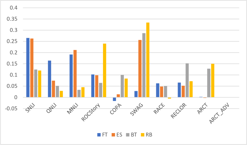
Figure 3: Four models’ hypothesis-only tests accuracies beyond vote by majority (hypo-only acc $-$ majority acc)

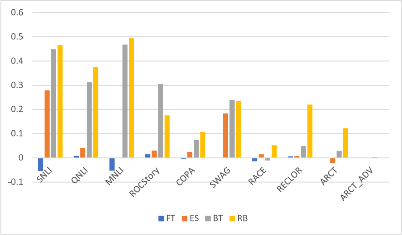
Figure 4: Four models’ full test accuracies above hypothesis-only tests accuracies (full acc $-$ hypo-only acc)

4.3 Cues in Datasets

We first filter the training and test data for each dataset using all the features defined in this paper. Left half of Table 3 shows the top 5 cues we have discovered as well as their cueness score for each of the 10 datasets. ARCT_adv is an adversarial dataset and is known to be well balanced on purpose. As a result, we only managed to find one cue which is OVERLAP and its cueness score is very low. This is not surprising, because OVERLAP is the only “second-order” feature in our list of linguistic features that is concerned with tokens in both the premise and hypothesis, and likely escaped from the data manipulation by the creator.

Dataset	Top Cues	Cueness	FT	ES	BT	RB
		%	($\Delta$)	($\Delta$)	($\Delta$)	($\Delta$)
SNLI	“sleeping”	13.95	30.3	6.81	5.34	4.87
	“no”	13.33	18.09	3.32	2.05	2.6
	“because”	9.24	18.89	4.88	5.61	4.31
	“friend”	8.82	22.96	6.66	3.51	3.05
	“movie”	7.73	16.64	0.06	9.47	-0.19
QNLI	“dioxide”	4.52	9.78	-0.06	4.97	10.56
	“denver”	4.26	13.59	7.14	2.23	3.11
	“kilometre”	4.24	4.85	6.43	4.67	2.55
	“mile”	3.95	7.16	15.64	-1.65	-6.65
	“newcastle”	3.8	3.44	12.0	0.89	-1.23
MNLI	“never”	10.4	29.15	26.41	9.86	10.6
	“no”	8.98	19.49	20.17	1.2	3.32
	“nothing”	8.98	25.5	26.84	5.11	4.32
	“any”	6.79	20.4	19.39	7.76	3.74
	“anything”	5.73	18.43	15.74	3.31	1.14
ROCStory	“threw”	12.99	1.28	4.69	10.88	0.97
	“now”	8.68	-10.01	14.51	1.75	5.69
	“found”	8.16	-2.31	4.45	5.12	-3.13
	“won”	7.71	2.43	0.74	1.05	5.51
	“like”	7.3	4.77	10.06	8.81	1.67
COPA	“went”	3.61	-10.83	6.46	7.92	1.04
	“got”	2.74	5.45	-9.89	-12.52	-10.3
	“for”	2.14	10.11	-1.89	9.05	11.58
	“with”	1.38	-15.64	-6.98	3.3	13.82
	TYPO	0.84	-12.46	-2.33	3.8	-8.22
SWAG	“football”	7.38	6.13	8.55	1.2	1.55
	“anxious”	6.65	7.55	-4.67	-6.66	-1.67
	“concerned”	6.19	12.6	4.58	8.27	-5.66
	“skull”	5.73	-2.77	0.49	8.43	3.49
	“cop”	5.01	2.79	5.3	-0.92	-0.04
RACE	“above”	13.74	8.73	-8.43	-0.22	-1.92
	“b”	12.84	16.97	-4.8	3.52	-3.45
	“c”	11.83	15.69	-6.94	8.6	-7.6
	“probably”	6.77	9.91	-0.06	-3.8	2.86
	“may”	4.2	7.75	-3.45	-6.67	-1.8
RECLOR	“over”	2.07	1.76	-2.94	-1.35	-4.12
	“result”	1.97	-3.29	-2.69	-1.78	-3.7
	“explanation”	1.81	-6.33	-1.73	-2.76	-7.24
	“proportion”	1.68	-5.64	-4.69	2.37	-2.16
	“produce”	1.4	4.54	-2.98	-14.36	-3.7
ARCT	“not”	3.74	-2.54	7.45	-0.97	-11.96
	NEGATION	2.85	3.49	10.04	6.28	-8.23
	“n’t”	2.52	10.3	5.89	9.49	4.84
	“always”	2.25	-4.66	38.21	-4.35	-8.26
	“doe”	2.06	-0.73	-3.69	-1.15	-7.22
ARCT_adv	OVERLAP	1.96e-10	1.65	-0.25	2.73	0.57
$\sum(|.|)$ (Model weakness)			469.8	361.4	227.7	216.2

Table 3: Datasets, their top 5 cues and 4 models biases $\Delta$ on them.

In most of the datasets, the top 5 cues discovered are word features, but besides OVERLAP, we do see NEGATION and TYPO showing up in the lists. In fact, SENTIMENT and NER features would have shown up if we expanded the list to top 10. It is also interesting to see several features previously reported to be biased by other works, such as “not” and NEGATION in ARCT, “no” in MNLI and SNLI, and “like” in ROCStory. Especially in MNLI, all the five cues discovered are related to negatively toned words, suggesting significant human artifacts in this datasets.

In the results, we also identify that some of the word cues are indicative of certain syntactic/semantic/sentiment patterns in the questions. For example, “because” in SNLI indicates a causal-effect structure; “like” in ROCStory indicates positive sentiment; “probably” and “may” in RACE indicate uncertainty, etc.

If we sum up the top 5 cueness scores for each dataset, we find that overall SNLI, RACE, ROCStory and MNLI carry more cueness than others, while ARCT_adv has the smallest cueness. This result is generally consistent with our findings in the hypothesis-only test (see Figure 3) earlier, though now we can pinpoint what causes the weaknesses in these four datasets. The only exception is SWAG, which didn’t emerge as a very weak dataset in the experiment here, but was found very biased in the hypothesis-only test. The reason is SWAG is the biggest dataset among the ten and we discovered more cues in it than the other 9 combined. Therefore, the top 5 cues are insufficient to represent the full scale of its weakness, which is showed by the hypothesis test as it gives the full picture.

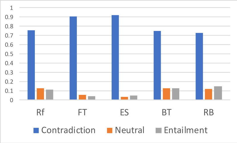
(a) Cue “no” in MNLI

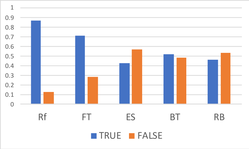
(b) Cue “above” in ARCT

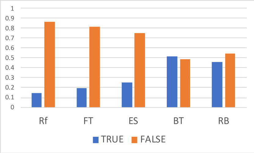
(c) Cue “threw” in ROCStory

Figure 5: Three test examples for distribution comparison with 4 different models

4.4 Biases in Models

For each feature and a dataset, we train four models on its original training set, and test the models on its full test set, feature-filtered test set, and neutral test set. We first show the result of “accuracy tests” in Table 3. If $\Delta$ is positive for a model on a feature, it means that the model exploits the existence of this feature. Conversely, the model exploits the non-existence of the this feature. A model is more robust against biases in the data, if $\Delta$ is close to zero. Therefore, the bottom of Table 3 shows that, across all 10 datasets, by the sum of the absolute values of $\Delta$, RoBERTA $<$ BERT $<$ ESIM $<$ FastText. This again is consistent with our hypothesis-only test earlier and the community’s common perception of these popular models. However, if we delve into individual datasets and features, situation can be a bit murkier.

For example, it seems that FastText tends to pick up more individual word cues than semantic cues, but more complex models such as BERT and RoBERTA appear to be more sensitive to structural features such as NEGATION and SENTIMENT, which are actually classes of words. This can be well explained by the way FastText is designed to model words more than syntactic or semantic structures.

The fact that FastText is strongly negatively correlated with TYPO is also interesting. We speculate that FastText might have been trained with a more orthodoxical vocabulary and thus less tolerant to typos in text.

We further invesigate the models using the “distribution test”. We show three insteresting findings in Figure 5. We observe that all models on cue “no” in MNLI achieve positive $\Delta$ in Table 3, and fastText in particular. Consistent with the “Accuracy test”, we find the predicting label distribution skewness is amplified in Figure 5(a) for fastText and ESIM - with “no” in sight, they prefer to predict “Contradiction” even more than the ground truth in training data. On the contrary, BERT and RoBERTA are only moderate in following the training data.

If cue “no” is very good at tricking the models, cue “above” is not as successful. Figure 5(b) shows that the distribution of predicting result for ESIM in ARCT is completely opposite to the training data. This explains while $\Delta=-8.43$ in Table 3 and demonstrates that models may not take advantage of the cue even though it is right there in the data. Similarly, the “flatness” in BERT and RoBERTA can also explain their low $\Delta$ values in Table 3.

The example of cue “threw” presents an outlier for BERT, because the distribution test result is inconsistent between the accuracy test: The accuracy deviation is very high for BERT, but its prediction distribution is flat. We haven’t seen a lot of such contradictory cases so far. But when it happens, as it is here, we give BERT the benefit of the doubt that it might not have exploited the cue “threw”.

5 Related Work

Our work is related to and, to some extent, comprises of elements in three research directions: spurious features analysis, bias calculation and dataset filtering.

Spurious features analysis has been increasingly studied recently. Much work Sharma et al. (2018); Srinivasan et al. (2018); Zellers et al. (2018) has observed that some NLP models can surprisingly get good results on natural language understanding questions in MCQ form without even looking at the stems of the questions. Such tests are called “hypothesis-only” tests in some works. Further, some research Sanchez et al. (2018) discovered that these models suffer from an insensitivity to certain small but semantically significant alterations in the hypotheses, leading to speculations that the hypothesis-only performance is due to simple statistical correlations between words in the hypothesis and the labels. Spurious features can be classified into lexicalized and unlexicalized Bowman et al. (2015): lexicalized features mainly contain indicators of n-gram tokens and cross-ngram tokens, while unlexicalized features involve word overlap, sentence length and BLUE score between the premise and the hypothesis.  Naik et al., 2018 refined the lexicalized classification to Negation, Numerical Reasoning, Spelling Error.  McCoy et al., 2019 refined the word overlap features to Lexical overlap, Subsequence and Constituent which also considers the syntactical structure overlap.  Sanchez et al., 2018 provided unseen tokens an extra lexicalized feature.

Bias calculation is concerned with methods to quantify the severity of the cues. Some work Clark et al. (2019); He et al. (2019); Yaghoobzadeh et al. (2019) attempted to encode the cue feature implicitly by hypothesis-only training or by extracting features associated with a certain label from the embeddings. Other methods compute the bias by statistical metrics. For example, Yu et al., 2020 used the probability of seeing a word conditioned on a specific label to rank the words by their biasness. LMI Schuster et al. (2019) was also used to evaluate cues and re-weight in some models. However, these works did not give the reason to use these metrics, one way or the other. Separately, Ribeiro et al., 2020 gave a test data augmentation method, without assessing the degree of bias in those datasets.

Dataset filtering is one way of achieving higher quality in datasets by reducing artifacts. In fact, datasets such as SWAG and RECLOR evaluated in this paper were produced using variants of this filter approach which iteratively perturb the data instances until a target model can no longer fit the resulting dataset well. Some methods Yaghoobzadeh et al. (2019), instead of preprocessing the data by removing biases, leave out samples with biases in the middle of training according to decision made between epoch to epoch. Bras et al., 2020 investigated model-based reduction of dataset cues and designed an algorithm using iterative training. Any model can be used in this framework. Although such an approach is more general and more efficient than human annotating, it heavily depends on the models. Unfortunately, different models may catch different cues. Thus, such methods may not be complete.

6 Conclusion

We develop a light-weight framework that evaluates the potential biases and cues in NLR multiple choice datasets and further shed light on the exploration of models at least from the perspective of the statistical cues. We experimented on a large range of datasets covering different tasks and conclude that the new evaluation framework is effective in discovering bias problems in both the datasets and some popular models.

References

- Bowman et al. [2015] Samuel Bowman, Gabor Angeli, Christopher Potts, and Christopher D Manning. A large annotated corpus for learning natural language inference. In EMNLP, pages 632–642, 2015.
- Bras et al. [2020] Ronan Le Bras, Swabha Swayamdipta, Chandra Bhagavatula, Rowan Zellers, Matthew E Peters, Ashish Sabharwal, and Yejin Choi. Adversarial filters of dataset biases. arXiv preprint arXiv:2002.04108, 2020.
- Clark et al. [2019] Christopher Clark, Mark Yatskar, and Luke Zettlemoyer. Don’t take the easy way out: Ensemble based methods for avoiding known dataset biases. In EMNLP-IJCNLP, pages 4060–4073, 2019.
- Gururangan et al. [2018] Suchin Gururangan, Swabha Swayamdipta, Omer Levy, Roy Schwartz, Samuel Bowman, and Noah A Smith. Annotation artifacts in natural language inference data. In NAACL-HLT, pages 107–112, 2018.
- He et al. [2019] He He, Sheng Zha, and Haohan Wang. Unlearn dataset bias in natural language inference by fitting the residual. EMNLP-IJCNLP, page 132, 2019.
- Jurafsky et al. [2020] Dan Jurafsky, Joyce Chai, Natalie Schluter, and Joel R. Tetreault, editors. ACL 2020, 2020.
- Lai et al. [2017] Guokun Lai, Qizhe Xie, Hanxiao Liu, Yiming Yang, and Eduard Hovy. RACE: Large-scale reading comprehension dataset from examinations. In EMNLP, pages 785–794, 2017.
- Lin [1991] J. Lin. Divergence measures based on the shannon entropy. IEEE Transactions on Information Theory, 37(1):145–151, 1991.
- McCoy et al. [2019] Tom McCoy, Ellie Pavlick, and Tal Linzen. Right for the wrong reasons: Diagnosing syntactic heuristics in natural language inference. In ACL, pages 3428–3448, 2019.
- Mostafazadeh et al. [2016] Nasrin Mostafazadeh, Nathanael Chambers, Xiaodong He, Devi Parikh, Dhruv Batra, Lucy Vanderwende, Pushmeet Kohli, and James Allen. A corpus and cloze evaluation for deeper understanding of commonsense stories. In NAACL-HLT, pages 839–849, 2016.
- Naik et al. [2018] Aakanksha Naik, Abhilasha Ravichander, Norman Sadeh, Carolyn Rose, and Graham Neubig. Stress test evaluation for natural language inference. In COLING, pages 2340–2353, 2018.
- Poliak et al. [2018] Adam Poliak, Jason Naradowsky, Aparajita Haldar, Rachel Rudinger, and Benjamin Van Durme. Hypothesis only baselines in natural language inference. In Joint Conference on Lexical and Computational Semantics, pages 180–191, 2018.
- Ribeiro et al. [2020] Marco Túlio Ribeiro, Tongshuang Wu, Carlos Guestrin, and Sameer Singh. Beyond accuracy: Behavioral testing of NLP models with checklist. In Proceedings of the 58th Annual Meeting of the Association for Computational Linguistics, ACL 2020, Online, July 5-10, 2020, pages 4902–4912, 2020.
- Roemmele et al. [2011] Melissa Roemmele, Cosmin Adrian Bejan, and Andrew S Gordon. Choice of plausible alternatives: An evaluation of commonsense causal reasoning. In AAAI Spring, 2011.
- Sanchez et al. [2018] Ivan Sanchez, Jeff Mitchell, and Sebastian Riedel. Behavior analysis of nli models: Uncovering the influence of three factors on robustness. In NAACL-HLT, pages 1975–1985, 2018.
- Schuster et al. [2019] Tal Schuster, Darsh J Shah, Yun Jie Serene Yeo, Daniel Filizzola, Enrico Santus, and Regina Barzilay. Towards debiasing fact verification models. arXiv preprint arXiv:1908.05267, 2019.
- Sharma et al. [2018] Rishi Sharma, James Allen, Omid Bakhshandeh, and Nasrin Mostafazadeh. Tackling the story ending biases in the story cloze test. In ACL, pages 752–757, 2018.
- Srinivasan et al. [2018] Siddarth Srinivasan, Richa Arora, and Mark Riedl. A simple and effective approach to the story cloze test. In NAACL-HLT, pages 92–96, 2018.
- Wang et al. [2018] Alex Wang, Amanpreet Singh, Julian Michael, Felix Hill, Omer Levy, and Samuel R Bowman. GLUE: A multi-task benchmark and analysis platform for natural language understanding. EMNLP, page 353, 2018.
- Yaghoobzadeh et al. [2019] Yadollah Yaghoobzadeh, Remi Tachet, TJ Hazen, and Alessandro Sordoni. Robust natural language inference models with example forgetting. arXiv preprint arXiv:1911.03861, 2019.
- Yu et al. [2020] Weihao Yu, Zihang Jiang, Yanfei Dong, and Jiashi Feng. ReClor: A reading comprehension dataset requiring logical reasoning. arXiv preprint arXiv:2002.04326, 2020.
- Zellers et al. [2018] Rowan Zellers, Yonatan Bisk, Roy Schwartz, and Yejin Choi. SWAG: A large-scale adversarial dataset for grounded commonsense inference. In EMNLP, pages 93–104, 2018.