A quantitative rigidity result
for a two-dimensional
Frenkel-Kontorova model

Abstract.

We consider a Frenkel-Kontorova system of harmonic oscillators in a two-dimensional Euclidean lattice and we obtain a quantitative estimate on the angular function of the equilibria. The proof relies on a PDE method related to a classical conjecture by E. De Giorgi, also in view of an elegant technique based on complex variables that was introduced by A. Farina.

In the discrete setting, a careful analysis of the reminders is needed to exploit this type of methodologies inspired by continuum models.

1. Introduction and statement of the main result

In [MR0001169], Yakov Frenkel and Tatiana Kontorova introduced a simple, but very effective, model to describe the atom dislocation dynamics of a crystal lattice. The model takes into account a pattern of particles with harmonic nearest neighbor interactions and subject to a substrate potential (in its simplest form, the potential is a periodic trigonometric function, but more general forcing terms can be also taken into account).

The simplest expression of the model by Frenkel and Kontorova consists of a harmonic chain of atoms of unit mass in a sinusoidal potential. The atoms are supposed to be at some (small) distance $h$ the ones from the others; hence, for simplicity, in dimension $1$, we can consider the location of the atoms at rest to be described by the lattice $h\mathbb{Z}$. The displacement $u_{i}(t)$, for each $i\in h\mathbb{Z}$ and $t\in\mathbb{R}$, describes the evolution of such a harmonic oscillator subject to nearest neighbor interactions (with Hooke constant $d>0$) and the sinusoidal potential according to the equation

(1.1) $${\displaystyle{\ddot{u}_{i}}+\sin u_{i}-\frac{d}{h^{2}}\,\big{(}u_{i+1}+u_{i-1}-2u_{i}\big{)}=0}.$$

Equilibrium configurations, i.e., stationary solutions of (1.1), are therefore obtained from the equation

(1.2) $${\displaystyle\sin u_{i}-\frac{d}{h^{2}}\,\big{(}u_{i+1}+u_{i-1}-2u_{i}\big{)}=0}.$$

Natural generalizations of (1.2) occur by considering the rest positions of the atoms in a plane (see Figure 1) and more general potentials than the sinusoid, possibly depending also on the position, in which case (1.2) is replaced by the more general form

(1.3) $$\sum_{j=1}^{2}\frac{u_{i+he_{j}}+u_{i-he_{j}}-2u_{i}}{h^{2}}=f(i,u_{i}),\qquad{\mbox{for all }}i\in h\mathbb{Z}^{2},$$

being $e_{1}:=(1,0)$ and $e_{2}:=(0,1)$. The detailed and simple mechanical interpretation of (1.3) is given by a system of particles constrained to move in the space along a vertical track, see Figure 1. More precisely, one assumes that the tracks are equally distributed in a square pattern, namely the intersection of the tracks and the ground level corresponds to the lattice $h\mathbb{Z}^{2}$. One also assumes that the closest particles are connected by elastic springs, say with Hooke constant equal to $d/h^{2}$. Moreover, the particles are subject to a potential which depends on the height of the particle and on the position of the vertical track along which the particle moves. In this way, if $u_{i}$ is the height of the particle located on the vertical trail placed at $i\in h\mathbb{Z}^{2}$, we denote by $V(i,u_{i})$ the corresponding external potential.

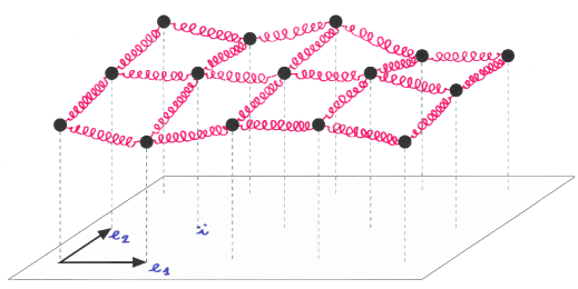
Figure 1. Mechanical interpretation of (1.3).

The total energy of this system is given by the formal series

(1.4) $${\mathcal{E}}(u):=\frac{d}{2h^{2}}\sum_{{i\in h\mathbb{Z}^{2}}\atop{j\in\{1,2\}}}|v_{i+he_{j}}-v_{i}|^{2}+\sum_{i\in h\mathbb{Z}^{2}}V(i,u_{i}),$$

where $v_{i}:=(i,u_{i})$ and $u=\{u_{i}\}_{i\in h\mathbb{Z}^{2}}$.

Observing that

$$|v_{i+he_{j}}-v_{i}|^{2}=(u_{i+he_{j}}-u_{i})^{2}+|(i+he_{j})-i|^{2}=(u_{i+he_{j}}-u_{i})^{2}+h^{2},$$

and the latter term is independent on the configuration, the equilibria of (1.4) coincide with those of

(1.5) $${\mathcal{F}}(u):=\frac{d}{2h^{2}}\sum_{{i\in h\mathbb{Z}^{2}}\atop{j\in\{1,2\}}}(u_{i+he_{j}}-u_{i})^{2}+\sum_{i\in h\mathbb{Z}^{2}}V(i,u_{i}).$$

The equilibria of (1.5) are found by considering the critical points for compact perturbations, leading to the equation

$$0=\langle D{\mathcal{F}}(u),\,\varphi\rangle=\frac{d}{h^{2}}\sum_{{i\in h\mathbb{Z}^{2}}\atop{j\in\{1,2\}}}(u_{i+he_{j}}-u_{i})(\varphi_{i+he_{j}}-\varphi_{i})+\sum_{i\in h\mathbb{Z}^{2}}\partial_{u_{i}}V(i,u_{i})\varphi_{i},$$

for every $\varphi=\{\varphi_{i}\}_{i\in h\mathbb{Z}^{2}}$ such that $\{\varphi_{i}\neq 0\}$ is a finite set.

Writing

$$\sum_{{i\in h\mathbb{Z}^{2}}\atop{j\in\{1,2\}}}(u_{i+he_{j}}-u_{i})(\varphi_{i+he_{j}}-\varphi_{i})$$

$$= \sum_{{i\in h\mathbb{Z}^{2}}\atop{j\in\{1,2\}}}(u_{i+he_{j}}-u_{i})\varphi_{i+he_{j}}-\sum_{{i\in h\mathbb{Z}^{2}}\atop{j\in\{1,2\}}}(u_{i+he_{j}}-u_{i})\varphi_{i}$$

$$= \sum_{{i\in h\mathbb{Z}^{2}}\atop{j\in\{1,2\}}}(u_{i}-u_{i-he_{j}})\varphi_{i}-\sum_{{i\in h\mathbb{Z}^{2}}\atop{j\in\{1,2\}}}(u_{i+he_{j}}-u_{i})\varphi_{i}$$

$$= \sum_{{i\in h\mathbb{Z}^{2}}\atop{j\in\{1,2\}}}(2u_{i}-u_{i+he_{j}}-u_{i+he_{j}})\varphi_{i},$$

we see that the equilibrium configurations satisfy

(1.6) $$\frac{d}{h^{2}}\,\sum_{j=1}^{2}(2u_{i}-u_{i+he_{j}}-u_{i+he_{j}})+\partial_{u_{i}}V(i,u_{i})=0,$$

which is precisely of the form given in (1.3).

In this paper, we will provide some “approximate symmetry” results for solutions of (1.3) under suitable structural assumptions. Roughly speaking, we will consider the angular function of the solution (i.e., the phase of the discrete increment of the solution) and control its weighted $\ell^{2}$-norm by the small parameter $h$ (and suitable structural constants). The weight function of such $\ell^{2}$-norm will also have a concrete meaning in the model, being the square of the discrete increment of the solution (the precise estimate will be formally stated in (1.22) below). In the formal limit $h\searrow 0$, estimates of this kind would entail a one-dimensional symmetry for the solution, yielding that the two-dimensional equilibrium configuration can be in fact represented by a one-dimensional function in some direction and the level sets of the solution are all straight lines. In this spirit, our result can be seen as a quantitative estimate on “how far the equilibrium configuration is from being one-dimensional” in the discrete setting and gives an optimal estimate on the perturbative effect played by the spatial parameter $h$.

We also point out that, in terms of atom dislocation theory, the Frenkel-Kontorova model can be considered as an “atomistic” description which can be rigorously related to the “microscopic” description of hybrid type given by the Peierls-Nabarro model, see [MR2852206]. See also [MR2035039] for a throughout presentation of the Frenkel-Kontorova model and for the detailed discussions of several applications to fields different than the theory of crystal dislocation (including, among the others, absorption, crowdions, magnetically ordered structures, Josephson junctions, hydrogen-bonded and DNA chains). In the dynamical systems setting, the equilibria of the Frenkel-Kontorova model with sinusoidal layer potential give rise to the Chirikov-Taylor map, and the continuum-limit is the sine-Gordon equation.

Given its constructive importance in the theory of crystal dislocation, its flexibility in a number of different applications, and its strong link to problems in dynamical systems and differential equations, the Frenkel-Kontorova model has been widely studied in the literature under different perspectives, and it has become a classical topic in several branches of statistical mechanics and in the analysis of harmonic oscillators on lattices, see e.g. [MR719055, MR719634, MR766107, MR1620543, MR2356117, MR3038682, MR3663614, MR3725364, MR3912645, MR4015338, MR4028786, MR4102235].

The point of view that we take in this article aims at describing the monotone solutions of a two-dimensional Frenkel-Kontorova model. The results obtained will be valid for every type of layer potential and their proof will rely on a number of analytical methods inspired by a classical conjecture by Ennio De Giorgi, see [MR533166] (see also [MR1775735, MR1637919, MR1655510, MR2480601, MR2757359, MR2728579, MR3488250] for several positive results in the direction of such conjecture, [MR2473304] for a counterexample in high dimension, and [MR2528756] for a survey on this topic).

Given $h\in(0,1]$ and $i\in h\mathbb{Z}^{2}$, for any $u:h\mathbb{Z}^{2}\to\mathbb{R}$, we set

(1.7) $${\mathcal{L}}u_{i}:=\sum_{j=1}^{2}\frac{u_{i+he_{j}}+u_{i-he_{j}}-2u_{i}}{h^{2}}.$$

We observe that, as $h\searrow 0$, the operator $\mathcal{L}$ recovers the usual Laplace operator.

Our main objective here is to consider solutions $u:h\mathbb{Z}^{2}\to\mathbb{R}$ of the equation (as in (1.3))

(1.8) $${\mathcal{L}}u_{i}=f(i,u_{i})\qquad{\mbox{ for all }}i\in h\mathbb{Z}^{2}.$$

We assume that $f:h\mathbb{Z}^{2}\times\mathbb{R}\to\mathbb{R}$ satisfies the following condition: there exist a function $L_{f}^{+}:h\mathbb{Z}^{2}\times\mathbb{R}\to\mathbb{R}$ and a finite positive constant $\kappa_{0}^{+}$ such that

(1.9) $$\sum_{j=1}^{2}\frac{\big{|}f(i+he_{j},u_{i+he_{j}})-f(i,u_{i})-L_{f}^{+}(i,u_{i})(u_{i+he_{j}}-u_{i})\big{|}}{h}\leqslant\kappa_{0}^{+}\,h,\quad\text{for all }\,i\in h\mathbb{Z}^{2}.$$

A significant particular case is given by a function $f:h\mathbb{Z}^{2}\times\mathbb{R}\to\mathbb{R}$ which is of class $C^{1}$ in the real variable, that is,

(1.10) $$f(i,\cdot)\in C^{1}(\mathbb{R}),\quad\text{for all }\,i\in h\mathbb{Z}^{2},$$

and satisfies (1.9) with $L_{f}^{+}(i,u_{i})=f^{\prime}(i,u_{i})$, where $f^{\prime}$ denotes the derivative of $f$ with respect to the real variable. In this case, (1.9) reads as

(1.11) $$\sum_{j=1}^{2}\frac{\big{|}f(i+he_{j},u_{i+he_{j}})-f(i,u_{i})-f^{\prime}(i,u_{i})(u_{i+he_{j}}-u_{i})\big{|}}{h}\leqslant\kappa_{0}^{+}\,h,\quad\text{for all }\,i\in h\mathbb{Z}^{2}.$$

We observe that assumption (1.11) states, in a quantitative way, that the dependence on the site of the nonlinearity $f$ is “negligible” (namely, the nonlinearity “mostly” depends on the state parameter $u_{i}$, rather than on $i$), see also page 1.3 for additional comments on this assumption in comparison with the continuous framework.

In this setting, we introduce the following notation: for every $j\in\{1,2\}$ and any $i\in h\mathbb{Z}^{2}$, we let

(1.12) $${\mathcal{D}}_{j}^{+}u_{i}:=\frac{u_{i+he_{j}}-u_{i}}{h}\qquad{\mbox{and}}\qquad{\mathcal{D}}_{j}^{-}u_{i}:=\frac{u_{i}-u_{i-he_{j}}}{h}.$$

The operators in (1.12) can be seen as discrete increments that converge to the standard derivative as $h\searrow 0$.

We will suppose that the solution $u$ of (1.8) satisfies some structural assumptions that we now describe in detail. Our main assumption is that

(1.13) $$\sum_{j=1}^{2}|u_{i+he_{j}}-u_{i}|^{2}>0,\qquad{\mbox{for all }}i\in h\mathbb{Z}^{2}.$$

Condition (1.13) requires that the “squared norm of the gradient” $\sum_{{1\leqslant j\leqslant 2}}|{\mathcal{D}}_{j}^{+}u_{i}|^{2}$ does not vanish, for all $i\in h\mathbb{Z}^{2}$.

In addition, we assume that

(1.14) $$\kappa_{1}^{+}:=\sup_{{i\in h\mathbb{Z}^{2}}\atop{1\leqslant j\leqslant 2}}|{\mathcal{D}}_{j}^{+}u_{i}|<+\infty.$$

Roughly speaking, one can consider (1.14) as a “Lipschitz” assumption on the solution $u$.

Following [MR2014827], it is convenient to use a complex variable notation, identifying $\mathbb{R}^{2}$ with $\mathbb{C}$. To this end, we set ${\mathcal{I}}:=\sqrt{-1}$ and

(1.15) $${U_{i}^{+}}:={\mathcal{D}}_{1}^{+}u_{i}+{\mathcal{I}}\,{\mathcal{D}}_{2}^{+}u_{i}=\frac{\big{(}u_{i+he_{1}}-u_{i}\big{)}+{\mathcal{I}}\,\big{(}u_{i+he_{2}}-u_{i}\big{)}}{h}.$$

Since by (1.13) we have that $|{U_{i}^{+}}|>0$ for any $i\in h\mathbb{Z}^{2}$, then ${U_{i}^{+}}/|{U_{i}^{+}}|$ is a function from $h\mathbb{Z}^{2}$ to the unit sphere $\mathcal{S}^{1}$ of $\mathbb{R}^{2}$. Thus, using a polar representation, there exists

(1.16) $$\vartheta^{+}_{i}\in\left(-\pi,\pi\right]$$

such that

$${U_{i}^{+}}=\rho_{i}^{+}\,e^{{\mathcal{I}}\vartheta^{+}_{i}},$$

where

$$\rho_{i}^{+}:=|{U_{i}^{+}}|.$$

In light of (1.14), we also know that

(1.17) $$\sup_{i\in h\mathbb{Z}^{2}}\rho_{i}^{+}=\sup_{i\in h\mathbb{Z}^{2}}|{U_{i}^{+}}|=\sup_{i\in h\mathbb{Z}^{2}}\big{(}\sqrt{|{\mathcal{D}}_{1}^{+}u_{i}|^{2}+|{\mathcal{D}}_{2}^{+}u_{i}|^{2}}\big{)}\leqslant\sqrt{2}\sup_{{i\in h\mathbb{Z}^{2}}\atop{1\leqslant j\leqslant 2}}|{\mathcal{D}}_{j}^{+}u_{i}|=\sqrt{2}\,\kappa_{1}^{+}.$$

We will now state some regularity assumptions on $\vartheta^{+}$ and $\rho$. First of all, we take some integrability hypotheses, supposing that

(1.18) $$\kappa_{2}^{+}:=\sum_{{1\leqslant j\leqslant 2}\atop{i\in h\mathbb{Z}^{2}}}(\rho_{i}^{+})^{2}\,\Big{(}|{\mathcal{D}}_{j}^{+}\vartheta^{+}_{i}|\,|{\mathcal{D}}_{j}^{+}({\mathcal{D}}_{j}^{+}\vartheta^{+})_{i-he_{j}}|+|{\mathcal{D}}_{j}^{-}\vartheta^{+}_{i}|\,|{\mathcal{D}}_{j}^{-}({\mathcal{D}}_{j}^{-}\vartheta^{+})_{i+he_{j}}|\Big{)}<+\infty.$$

We observe that (1.18) is satisfied provided that the angular function $\vartheta^{+}$ “does not oscillate” too much at infinity. We now take additional assumptions in this spirit by supposing that $\vartheta^{+}$ is suitably close to a limit angle at infinity. To this end, for all $j\in\{1,2\}$ and all $i\in h\mathbb{Z}^{2}$, we introduce the notation

(1.19) $${\mathcal{L}}_{j}{u}_{i}:=\frac{u_{i+he_{j}}+u_{i-he_{j}}-2u_{i}}{h^{2}}.$$

Notice that

(1.20) $${\mathcal{L}}:={\mathcal{L}}_{1}+{\mathcal{L}}_{2}.$$

We assume that there exists $\vartheta^{+}_{\infty}\in\left(-\pi,\pi\right]$ such that the following assumptions hold true:

(1.21) $$\begin{split}&\kappa_{3}^{+}:=\sum_{{1\leqslant j\leqslant 2}\atop{i\in h\mathbb{Z}^{2}}}(\rho_{i}^{+})^{2}\,\Big{(}|{\mathcal{D}}_{j}^{+}\vartheta^{+}_{i}|^{3}+|{\mathcal{D}}_{j}^{-}\vartheta^{+}_{i}|^{3}\Big{)}\,|\vartheta^{+}_{i}-\vartheta^{+}_{\infty}|<+\infty,\\ &\kappa_{4}^{+}:=\sum_{{1\leqslant j\leqslant 2}\atop{i\in h\mathbb{Z}^{2}}}\rho_{i}^{+}\,\big{(}|{\mathcal{D}}_{j}^{+}\rho_{i}^{+}|\;|{\mathcal{D}}_{j}^{+}\vartheta^{+}_{i}|^{2}+|{\mathcal{D}}_{j}^{-}\rho_{i}^{+}|\;|{\mathcal{D}}_{j}^{-}\vartheta^{+}_{i}|^{2}\big{)}\,|\vartheta^{+}_{i}-\vartheta^{+}_{\infty}|<+\infty\\ &\kappa_{5}^{+}:=\kappa_{0}^{+}\,\sum_{i\in h\mathbb{Z}^{2}}\rho_{i}^{+}\,|\vartheta^{+}_{i}-\vartheta^{+}_{\infty}|<+\infty,\\ &\kappa_{6}^{+}:=\sum_{{1\leqslant j\leqslant 2}\atop{i\in h\mathbb{Z}^{2}}}\Big{(}|{\mathcal{D}}_{j}^{+}(\rho_{i}^{+})^{2}|\,|{\mathcal{D}}_{j}^{+}({\mathcal{D}}_{j}^{+}\vartheta^{+})_{i}|+|{\mathcal{D}}_{j}^{-}(\rho_{i}^{+})^{2}|\,|{\mathcal{D}}_{j}^{-}({\mathcal{D}}_{j}^{-}\vartheta^{+})_{i}|+h(\rho_{i}^{+})^{2}\,|{\mathcal{L}}^{2}_{j}\vartheta^{+}_{i}|\Big{)}\,|\vartheta^{+}_{i}-\vartheta^{+}_{\infty}|<+\infty,\\ &\kappa_{7}^{+}:=\sum_{{1\leqslant j\leqslant 2}\atop{i\in h\mathbb{Z}^{2}}}\Big{(}|{\mathcal{D}}_{j}^{+}\rho_{i}^{+}|^{2}\,|{\mathcal{D}}_{j}^{+}\vartheta^{+}_{i}|+|{\mathcal{D}}_{j}^{-}\rho_{i}^{+}|^{2}\,|{\mathcal{D}}_{j}^{-}\vartheta^{+}_{i}|\Big{)}\,|\vartheta^{+}_{i}-\vartheta^{+}_{\infty}|<+\infty.\end{split}$$

In this setting, our main result here is as follows:

Theorem 1.1.

Let $f:h\mathbb{Z}^{2}\times\mathbb{R}\to\mathbb{R}$ satisfy (1.9). Let $u:h\mathbb{Z}^{2}\to\mathbb{R}$ be a solution of (1.8), satisfying (1.13), (1.14), (1.18), and (1.21).

Then,

(1.22) $$\sum_{{1\leqslant j\leqslant 2}\atop{i\in h\mathbb{Z}^{2}}}(\rho_{i}^{+})^{2}\;\Big{(}|{\mathcal{D}}_{j}^{+}\vartheta^{+}_{i}|^{2}+|{\mathcal{D}}_{j}^{-}\vartheta^{+}_{i}|^{2}\Big{)}\leqslant Ch,$$

where $C>0$ is given by

(1.23) $$C:=4\left(\kappa_{2}^{+}+2e^{2\pi}\kappa_{3}^{+}+2e^{2\pi}\kappa_{4}^{+}+2\kappa_{5}^{+}+\kappa_{6}^{+}+\kappa_{7}^{+}\right).$$

As a variant of Theorem 1.1, one can also consider ${U_{i}^{-}}:={\mathcal{D}}_{1}^{-}u_{i}+{\mathcal{I}}\,{\mathcal{D}}_{2}^{-}u_{i}$ and $\rho_{i}^{-}:=|{U_{i}^{-}}|$. Thus, under the assumption that

(1.24) $$\sum_{j=1}^{2}|u_{i-he_{j}}-u_{i}|^{2}>0,\qquad{\mbox{for all }}i\in h\mathbb{Z}^{2},$$

we have that $\rho_{i}^{-}\neq 0$ for every $i\in h\mathbb{Z}^{2}$, whence we can define $\vartheta^{-}_{i}\in\left(-\pi,\pi\right]$ such that ${U_{i}^{-}}=\rho_{i}^{-}\,e^{{\mathcal{I}}\vartheta^{-}_{i}}$. To obtain a full counterpart of Theorem 1.1 that takes into account “both positive and negative increments” it is convenient to complement (1.9) with the assumption that there exist a function $L_{f}^{-}:h\mathbb{Z}^{2}\times\mathbb{R}\to\mathbb{R}$ and a constant $\kappa_{0}^{-}>0$ such that

(1.25) $$\sum_{j=1}^{2}\frac{\big{|}f(i,u_{i})-f(i-he_{j},u_{i-he_{j}})-L_{f}^{-}(i,u_{i})(u_{i}-u_{i-he_{j}})\big{|}}{h}\leqslant\kappa_{0}^{-}\,h,\quad\text{for all }\,i\in h\mathbb{Z}^{2}.$$

Analogously, assumptions (1.14), (1.18), and (1.21) will be combined with the following conditions:

(1.26) $$\begin{split}&\kappa_{1}^{-}:=\sup_{{i\in h\mathbb{Z}^{2}}\atop{1\leqslant j\leqslant 2}}|{\mathcal{D}}_{j}^{-}u_{i}|<+\infty,\\ &\kappa_{2}^{-}:=\sum_{{1\leqslant j\leqslant 2}\atop{i\in h\mathbb{Z}^{2}}}(\rho_{i}^{-})^{2}\,\Big{(}|{\mathcal{D}}_{j}^{+}\vartheta^{-}_{i}|\,|{\mathcal{D}}_{j}^{+}({\mathcal{D}}_{j}^{+}\vartheta^{-})_{i-he_{j}}|+|{\mathcal{D}}_{j}^{-}\vartheta^{-}_{i}|\,|{\mathcal{D}}_{j}^{-}({\mathcal{D}}_{j}^{-}\vartheta^{-})_{i+he_{j}}|\Big{)}<+\infty,\\ &\kappa_{3}^{-}:=\sum_{{1\leqslant j\leqslant 2}\atop{i\in h\mathbb{Z}^{2}}}(\rho_{i}^{-})^{2}\,\Big{(}|{\mathcal{D}}_{j}^{+}\vartheta^{-}_{i}|^{3}+|{\mathcal{D}}_{j}^{-}\vartheta^{-}_{i}|^{3}\Big{)}\,|\vartheta^{-}_{i}-\vartheta^{-}_{\infty}|<+\infty,\\ &\kappa_{4}^{-}:=\sum_{{1\leqslant j\leqslant 2}\atop{i\in h\mathbb{Z}^{2}}}\rho_{i}^{-}\,\big{(}|{\mathcal{D}}_{j}^{+}\rho_{i}^{-}|\;|{\mathcal{D}}_{j}^{+}\vartheta^{-}_{i}|^{2}+|{\mathcal{D}}_{j}^{-}\rho_{i}^{-}|\;|{\mathcal{D}}_{j}^{-}\vartheta^{-}_{i}|^{2}\big{)}\,|\vartheta^{-}_{i}-\vartheta^{-}_{\infty}|<+\infty\\ &\kappa_{5}^{-}:=\kappa_{0}^{-}\,\sum_{i\in h\mathbb{Z}^{2}}\rho_{i}^{-}\,|\vartheta^{-}_{i}-\vartheta^{-}_{\infty}|<+\infty,\\ &\kappa_{6}^{-}:=\sum_{{1\leqslant j\leqslant 2}\atop{i\in h\mathbb{Z}^{2}}}\Big{(}|{\mathcal{D}}_{j}^{+}(\rho_{i}^{-})^{2}|\,|{\mathcal{D}}_{j}^{+}({\mathcal{D}}_{j}^{+}\vartheta^{-})_{i}|+|{\mathcal{D}}_{j}^{-}(\rho_{i}^{-})^{2}|\,|{\mathcal{D}}_{j}^{-}({\mathcal{D}}_{j}^{-}\vartheta^{-})_{i}|+h(\rho_{i}^{-})^{2}\,|{\mathcal{L}}^{2}_{j}\vartheta^{-}_{i}|\Big{)}\,|\vartheta^{-}_{i}-\vartheta^{-}_{\infty}|<+\infty,\\ &\kappa_{7}^{-}:=\sum_{{1\leqslant j\leqslant 2}\atop{i\in h\mathbb{Z}^{2}}}\Big{(}|{\mathcal{D}}_{j}^{+}\rho_{i}^{-}|^{2}\,|{\mathcal{D}}_{j}^{+}\vartheta^{-}_{i}|+|{\mathcal{D}}_{j}^{-}\rho_{i}^{-}|^{2}\,|{\mathcal{D}}_{j}^{-}\vartheta^{-}_{i}|\Big{)}\,|\vartheta^{-}_{i}-\vartheta^{-}_{\infty}|<+\infty.\end{split}$$

for some $\vartheta^{-}_{\infty}\in\left(-\pi,\pi\right]$. Then, we set $\kappa_{m}:=\kappa_{m}^{+}+\kappa_{m}^{-}$ for all $m\in\{0,\dots,7\}$ and we have the following rigidity result:

Theorem 1.2.

Let $f:h\mathbb{Z}^{2}\times\mathbb{R}\to\mathbb{R}$ satisfy (1.9) and (1.25).

Let $u:h\mathbb{Z}^{2}\to\mathbb{R}$ be a solution of (1.8), satisfying (1.13), (1.14), (1.18), (1.21), (1.24), and (1.26).

Then,

(1.27) $$\sum_{{1\leqslant j\leqslant 2}\atop{i\in h\mathbb{Z}^{2}}}\Big{[}(\rho_{i}^{+})^{2}\;\Big{(}|{\mathcal{D}}_{j}^{+}\vartheta^{+}_{i}|^{2}+|{\mathcal{D}}_{j}^{-}\vartheta^{+}_{i}|^{2}\Big{)}+(\rho_{i}^{-})^{2}\;\Big{(}|{\mathcal{D}}_{j}^{+}\vartheta^{-}_{i}|^{2}+|{\mathcal{D}}_{j}^{-}\vartheta^{-}_{i}|^{2}\Big{)}\Big{]}\leqslant Ch,$$

where $C>0$ is given by

$$C:=4\left(\kappa_{2}+2e^{2\pi}\kappa_{3}+2e^{2\pi}\kappa_{4}+2\kappa_{5}+\kappa_{6}+\kappa_{7}\right).$$

We observe that estimates (1.22) and (1.27) provide quantitative rigidity results. Indeed, in the formal limit as $h\searrow 0$, if $Ch$ tends to $0$ then the quantities

(1.28) $$\sum_{{1\leqslant j\leqslant 2}\atop{i\in h\mathbb{Z}^{2}}}(\rho_{i}^{\pm})^{2}\;\Big{(}|{\mathcal{D}}_{j}^{+}\vartheta^{\pm}_{i}|^{2}+|{\mathcal{D}}_{j}^{-}\vartheta^{\pm}_{i}|^{2}\Big{)}$$

become infinitesimal. In particular, the vanishing of (1.28) would correspond to a constant direction of the gradient (in all regions where the gradient itself does not vanish). See Lemma 1.3 for a precise formulation of the one-dimensional symmetry property related to these conditions.

Theorem 1.2 is a perfect counterpart of Theorem 1.1, therefore in this paper we will mostly focus on the first of these results.

We observe that, for a given $h\in(0,1]$ (i.e., even without taking limits), a simple byproduct of (1.22) and of the fact, due to (1.13), that $(\rho_{i}^{+})^{2}=h^{-2}\sum\limits_{j=1}^{2}|u_{i+he_{j}}-u_{i}|^{2}>0$ is that, for all $i\in h\mathbb{Z}^{2}$ and all $j\in\{1,2\}$,

$$|\vartheta^{+}_{i+he_{j}}-\vartheta^{+}_{i}|^{2}=h^{2}|{\mathcal{D}}_{j}^{+}\vartheta^{+}_{i}|^{2}\leqslant\frac{Ch^{3}}{(\rho_{i}^{+})^{2}}=\frac{Ch^{5}}{\sum\limits_{j=1}^{2}|u_{i+he_{j}}-u_{i}|^{2}},$$

which gives an explicit bound on the discrete variation of the angular function in terms of the size of the lattice and the assumption in (1.13).

In this spirit, we mention that assumptions (1.18) and (1.21) are, a-posteriori, consistent with the (approximate) constancy of the angular function, in the sense that if $\vartheta^{+}$ is constant, then conditions (1.18) and (1.21) are obviously fulfilled.

We point out that the summability conditions in (1.18) and (1.21) are specific for the discrete case and do not have a clear counterpart in the continuous case. As a matter of fact, roughly speaking, at a formal level, the quantities introduced in (1.18) and (1.21) are multiplied by $h$ in (1.22) and therefore this product formally disappears in the continuous limit.

On the other hand, one could also consider a continuous analogue of the discrete conditions in (1.18) and (1.21) simply by replacing increments by derivatives and sums with integrals: this formal passage to the limit would correspond to several integrability conditions which, as far as we are aware of, do not appear in the literature related to symmetry properties of semilinear elliptic partial differential equations. However all these integrability conditions would be obviously satisfied by one-dimensional solutions (since the corresponding phase of the gradient would be constant in space), therefore, a posteriori, these conditions do not trivialize the space of solutions in the continuous setting.

We observe that Theorems 1.1 and 1.2 possess a neat mechanical interpretation according to Figure 1. Indeed, recalling (1.6), potentials of particular interests are the ones only depending on the height (say, of the form $V(i,u_{i})=\hat{V}(u_{i})$), and for instance the gravitational potential is of this form.

And it is of course of particular interest to understand equilibrium configurations when the tracks become denser and denser (that is for smaller and smaller $h$).

Theorems 1.1 and 1.2 address quantitatively this question, by establishing that for “very dense” tracks and potentials depending “almost only on the height” then equilibria are “almost flat” configurations, in the sense that their increments have “almost constant” direction in the plane – the precise quantification of this rough statement being given by the bound in (1.22).

We also provide an observation of geometric flavor, stating that when the left-hand side of (1.27) vanishes identically the function $u:h\mathbb{Z}^{2}\to\mathbb{R}$ is one-dimensional, in the sense that it can be reconstructed by a one-dimensional function $\widetilde{u}:h\mathbb{Z}\to\mathbb{R}$ (and this also highlights the fact that Theorem 1.2 can be seen as a one-dimensional, quantitative, stability result).

Lemma 1.3.

Let $u:h\mathbb{Z}^{2}\to\mathbb{R}$ be such that

(1.29) $$\mathcal{D}^{+}_{2}u_{i}\neq 0\qquad{\mbox{and}}\qquad\mathcal{D}^{-}_{2}u_{i}\neq 0$$

for all $i\in h\mathbb{Z}^{2}$, and assume that

(1.30) $$\sum_{{1\leqslant j\leqslant 2}\atop{i\in h\mathbb{Z}^{2}}}\Big{[}(\rho_{i}^{+})^{2}\;\Big{(}|{\mathcal{D}}_{j}^{+}\vartheta^{+}_{i}|^{2}+|{\mathcal{D}}_{j}^{-}\vartheta^{+}_{i}|^{2}\Big{)}+(\rho_{i}^{-})^{2}\;\Big{(}|{\mathcal{D}}_{j}^{+}\vartheta^{-}_{i}|^{2}+|{\mathcal{D}}_{j}^{-}\vartheta^{-}_{i}|^{2}\Big{)}\Big{]}=0.$$

Then, there exist $\widetilde{u}:h\mathbb{Z}\to\mathbb{R}$, $c^{+}$, $c^{-}\in\mathbb{R}$, such that

(1.31) $$u_{(hk,hm)}=\sum_{j=0}^{|k|}{\binom{|k|}{j}}(c^{\sigma_{k}})^{j}\,(1-c^{\sigma_{k}})^{|k|-j}\,\widetilde{u}_{h(m+\sigma_{k}j)},$$

for every $k$, $m\in\mathbb{Z}$, where

$$\sigma_{k}:=\begin{cases}+&{\mbox{ if }}k>0,\\ -&{\mbox{ if }}k<0,\\ 0&{\mbox{ if }}k=0,\end{cases}$$

and we understand $c^{\sigma_{0}}=c^{0}=1$.

In addition,

(1.32) $$\frac{u_{i\pm he_{1}}-u_{i}}{u_{i\pm he_{2}}-u_{i}}=c^{\pm}\qquad{\mbox{for all }}i\in h\mathbb{Z}^{2}.$$

We stress that (1.31) states that the knowledge of the one-dimensional function $\widetilde{u}$ is sufficient for the complete knowledge of the two-dimensional function $u$. Moreover, the identity in (1.32) can be seen as the discrete counterparts of continuous identities of the type $\frac{\partial_{1}u}{\partial_{2}u}={\rm const}$ which characterizes smooth functions in $\mathbb{R}^{2}$ whose level sets are parallel straight lines.

We also remark that (1.31) can be seen, formally, as a discrete analogue of the continuous identity

(1.33) $$u(x_{1},x_{2})=\widetilde{u}(cx_{1}+x_{2}),$$

for some constant $c$, which expresses the fact the the function $u:\mathbb{R}^{2}\to\mathbb{R}$ is actually depending on one Euclidean variable in the direction $(c,1)$: see Appendix A for further comments on this formal relation.

There is however an interesting conceptual difference between the discrete relation in (1.31) and its continuous counterpart in (1.33). Indeed, in the continuous case, the value of $u$ at a given point, say $(x_{1},x_{2})$, is reconstructed by the knowledge of the value of its one-dimensional representation $\widetilde{u}$ at precisely one specific point (namely, in light of (1.33), at the point $cx_{1}+x_{2}$). Instead, in the discrete case, the value of $u$ at a given site, for instance $(hk,hm)$ with $k$, $m\in\mathbb{Z}$ and $k>0$, is reconstructed via (1.31) by the values of its one-dimensional representation $\widetilde{u}$ at several sites, namely $(0,hm)$, $(h,hm)$, $\dots$, $(hk,hm)$ (though of course this nonlocal effect disappears in the continuous limit of infinitesimal $h$).

We emphasize that the symmetry results in the continuous case are necessarily obtained for potentials of the form $f(u)$ that only depend on $u$. Here, the quantitative nature of our result allows to consider potentials of the form $f(i,u_{i})$ that also depend on the position $i\in h\mathbb{Z}^{2}$. Notice that, assumption (1.11) quantitatively controls the dependence of $f$ on $i$: in the formal limit as $h\searrow 0$, (1.11) informs us that such dependence tends to disappear, in accordance with the symmetry results known in the continuous case.

We also notice that assumptions (1.10) and (1.11) (and hence in particular (1.9)) are always satisfied by any semilinearity of the form $f(i,u_{i})=\hat{f}(u_{i})$ (only depending on $u$), provided that

(1.34) $$\hat{f}\in C^{2}(\mathbb{R})\quad\text{ and }\quad\|\hat{f}^{\prime\prime}\|_{L^{\infty}(\mathbb{R})}<+\infty.$$

Indeed, in this case (1.10) trivially holds true. Moreover, we have

$$\begin{split}&\sum_{j=1}^{2}\frac{\big{|}f(i+he_{j},u_{i+he_{j}})-f(i,u_{i})-f^{\prime}(i,u_{i})(u_{i+he_{j}}-u_{i})\big{|}}{h}\\ =\,&\sum_{j=1}^{2}\frac{\big{|}\hat{f}(u_{i+he_{j}})-\hat{f}(u_{i})-\hat{f}^{\prime}(u_{i})(u_{i+he_{j}}-u_{i})\big{|}}{h}\\ =\,&\frac{1}{h}\sum_{j=1}^{2}\left|\int_{u_{i}}^{u_{i+he_{j}}}\big{(}\hat{f}^{\prime}(t)-\hat{f}^{\prime}(u_{i})\big{)}\,dt\right|\\ \leqslant\,&\frac{\|\hat{f}^{\prime\prime}\|_{L^{\infty}(\mathbb{R})}}{2h}\sum_{j=1}^{2}\,|u_{i+he_{j}}-u_{i}|^{2}\\ =\,&\frac{\|\hat{f}^{\prime\prime}\|_{L^{\infty}(\mathbb{R})}\,h}{2}\sum_{j=1}^{2}|{\mathcal{D}}_{j}^{+}u_{i}|^{2},\end{split}$$

and hence (1.11) holds true with $\kappa_{0}^{+}=(\kappa_{1}^{+})^{2}\,\|\hat{f}^{\prime\prime}\|_{L^{\infty}(\mathbb{R})}$.

We stress that, in our setting, an exact symmetry result analogous to that in the continuous case cannot be obtained, as the examples in Section 4 show. In particular, Examples 4.2 and 4.3 show that such an exact symmetry result cannot hold true in the discrete case, even if we restrict our analysis to the case of source terms $f(i,u_{i})=\hat{f}(u_{i})$ that do not depend on the position and satisfy (1.9).

All the examples in Section 4 also show that the rate of convergence of the estimate (1.22) in the formal limit $h\searrow 0$ is optimal in the sense that, in this case, right-hand side and left-hand side are of the same order of $h$.

Here, we will focus on the proof of Theorem 1.1 (the proof of Theorem 1.2 would then follow by a spatial symmetry argument). The approach to prove Theorem 1.1 in this paper relies on the complex variable method introduced in [MR2014827] to deal with the original De Giorgi’s problem in [MR533166] (in our setting, the discrete structure of the lattices requires a careful estimate on the discrepancies between differentiable functions and finite increments and concrete bounds on the approximations performed).

The strategy of the proof of Theorem 1.1 is based on a useful identity for the increments of the solution (roughly speaking, this method would be the discrete counterpart of the study of a “linearized equation” in the continuum models setting). This step is accomplished in Lemma 3.1. Then, the desired result is obtained by an application of a new discrete quantitative Liouville-type theorem (see the proof of Theorem 1.1).

The complex variable formalism introduced in [MR2014827] reveals interesting cancellations when looking at the imaginary parts of this type of equations: this is an interesting fact which makes it possible to exploit this method to all layer potentials, without structural restrictions, since the potential plays no role in the imaginary part of the limit equation in the continuum model case, and in the discrete case it only plays a role in the estimates of the remainders (therefore, in our framework, assumption (1.9) on the source term $f$ is required to get the error estimates, but no condition on the shape of $f$ is necessary to obtain Theorem 1.1).

The technical details of the proof of Theorem 1.1 are presented in Section 3 and exploit also auxiliary computations of elementary flavor that are collected in Section 2. Section 3 also contains the proof of Lemma 1.3. Then, in Section 4 we provide some examples showing the optimality of our estimates.

In future projects, we aim at developing the method of this paper to obtain other forms of approximate counterparts of De Giorgi’s conjecture in the discrete setting especially by addressing approximation results of geometrical nature and possibly detecting suitable hypotheses which make level sets of discrete solutions appropriately close to a line, or to a portion of a line. Besides the methods in [MR1655510], for this it will be convenient to revisit the geometric Poincaré formula in [MR1650327], as utilized in [MR2483642], since this type of inequalities provide natural bounds for the total curvature of the level sets of the solutions. This technique could also lead to the study of long-range interaction models, possibly involving infinitely many site interactions with suitable decay at infinity, by taking advantage of integro-differential versions of the geometric Poincaré formula, as done in [MR3469920] for the continuous case.

We conclude this introduction by pointing out a substantial difference between the discrete and the continuous settings. In the continuous case, if $u$ is a $C^{2}(\mathbb{R}^{2})$ function with $|\nabla u|>0$, then $\nabla u/|\nabla u|\in C^{1}(\mathbb{R}^{2},\mathcal{S}^{1})$. In that setting, in place of $\vartheta^{+}$ we have $\vartheta$, which is a $C^{1}(\mathbb{R}^{2})$ function satisfying $\nabla u=|\nabla u|e^{i\vartheta}$. Notice that $\vartheta$ may be unbounded in the continuous case. This necessarily leads to require further assumptions on $u$ such as monotonicity in a given direction, or more generally, stability (see [MR2528756]). We recall that a sufficient condition to perform Farina’s proof is given by the boundedness of $\vartheta^{+}$ (see [MR2014827] and [MR2528756]), which is surely verified for instance if $u$ is increasing in a given direction (say $e_{2}$). Indeed, the monotonicity of $u$ in the $e_{2}$ direction guarantees that $\nabla u$ does not “turn backwards”, that is $\vartheta^{+}\in\left[0,\pi\right]$, and so in particular that $\vartheta^{+}$ is bounded.

The discrete setting provides here an interesting difference with respect to the continuous case. Indeed, being $\vartheta^{+}_{i}$ a function defined on $h\mathbb{Z}^{2}$, no continuity notions come into play, and one is free to choose all the angles in $(-\pi,\pi]$ (that is, such a normalization does not conflict with any continuity assumption in the discrete case). For this reason, in our setting, if (1.13) holds true, then one can always define the polar angle, and renormalize it to fulfill (1.16). In particular, in our framework, no monotonicity or stability assumption is required, in contrast with the models in the continuum.

We also stress that assumption (1.13) is obviously satisfied if we assume

(1.35) $$u_{i+he_{2}}>u_{i}\qquad{\mbox{for all }}i\in h\mathbb{Z}^{2},$$

that is a discrete “monotonicity assumption” in the vertical direction.

2. Toolbox

This section contains some ancillary observations, to be used in the proof of Theorem 1.1 which is contained in Section 3. We start by computing the operator ${\mathcal{L}}$ on the product of two functions. For this, if $f$, $g:h\mathbb{Z}^{2}\to\mathbb{R}$, we write that $\psi:=fg$ to mean that, for any $i\in h\mathbb{Z}^{2}$, we have $\psi_{i}:=f_{i}g_{i}$. We have the following product rule for the increment quotients introduced in (1.12):

Lemma 2.1.

Let $f$, $g:h\mathbb{Z}^{2}\to\mathbb{R}$. Then, for all $j\in\{1,2\}$,

(2.1) $${\mathcal{D}}_{j}^{+}(fg)_{i}=\frac{f_{i+he_{j}}+f_{i}}{2}\;{\mathcal{D}}_{j}^{+}g_{i}+\frac{g_{i+he_{j}}+g_{i}}{2}\;{\mathcal{D}}_{j}^{+}f_{i}$$

and

(2.2) $${\mathcal{D}}_{j}^{-}(fg)_{i}=\frac{f_{i-he_{j}}+f_{i}}{2}\;{\mathcal{D}}_{j}^{-}g_{i}+\frac{g_{i-he_{j}}+g_{i}}{2}\;{\mathcal{D}}_{j}^{-}f_{i}.$$

Proof.

We focus on the proof of (2.2), since the proof of (2.1) is similar. To this end, we point out that

$${\mathcal{D}}_{j}^{-}(fg)_{i} = \frac{(fg)_{i}-(fg)_{i-he_{j}}}{h}$$

$$= \frac{f_{i}(g_{i}-g_{i-he_{j}})+g_{i-he_{j}}(f_{i}-f_{i-he_{j}})}{h}$$

$$= f_{i}\,{\mathcal{D}}_{j}^{-}g_{i}+g_{i-he_{j}}\,{\mathcal{D}}_{j}^{-}f_{i}.$$

Also, exchanging the roles of $f$ and $g$,

$${\mathcal{D}}_{j}^{-}(fg)_{i} = g_{i}\,{\mathcal{D}}_{j}^{-}f_{i}+f_{i-he_{j}}\,{\mathcal{D}}_{j}^{-}g_{i},$$

and therefore

$$2{\mathcal{D}}_{j}^{-}(fg)_{i} = \Big{(}f_{i}\,{\mathcal{D}}_{j}^{-}g_{i}+g_{i-he_{j}}\,{\mathcal{D}}_{j}^{-}f_{i}\Big{)}+\Big{(}g_{i}\,{\mathcal{D}}_{j}^{-}f_{i}+f_{i-he_{j}}\,{\mathcal{D}}_{j}^{-}g_{i}\Big{)}$$

$$= (g_{i-he_{j}}+g_{i})\,{\mathcal{D}}_{j}^{-}f_{i}+(f_{i-he_{j}}+f_{i})\,{\mathcal{D}}_{j}^{-}g_{i},$$

from which (2.2) plainly follows. ∎

It is also interesting to observe that the increments defined in (1.12) produce by iteration (a suitable translation and projection of) the operator in (1.7), namely, recalling the notation in (1.19), the following result holds true:

Lemma 2.2.

Let $f:h\mathbb{Z}^{2}\to\mathbb{R}$. Then,

(2.3) $${\mathcal{D}}_{j}^{+}({\mathcal{D}}_{j}^{+}f)_{i}={\mathcal{L}}_{j}f_{i+he_{j}}$$

and

(2.4) $${\mathcal{D}}_{j}^{-}({\mathcal{D}}_{j}^{-}f)_{i}={\mathcal{L}}_{j}f_{i-he_{j}}.$$

Proof.

We see that, for every $j\in\{1,2\}$,

$${\mathcal{D}}_{j}^{-}({\mathcal{D}}_{j}^{-}f)_{i} = \frac{{\mathcal{D}}_{j}^{-}f_{i}-{\mathcal{D}}_{j}^{-}f_{i-he_{j}}}{h}$$

$$= \frac{(f_{i}-f_{i-he_{j}})-(f_{i-he_{j}}-f_{i-2he_{j}})}{h^{2}}$$

$$= \frac{f_{i-2he_{j}}+f_{i}-2f_{i-he_{j}}}{h^{2}}.$$

This proves (2.4), and the proof of (2.3) is similar. ∎

We remark that it is not always convenient to sum (2.3) and (2.4) over $j\in\{1,2\}$, since the right-hand side depends on $j$ in such a way that the operator ${\mathcal{L}}$ does not appear straight away after such a summation.

We also present the following useful computation:

Lemma 2.3.

Let $f$, $g:h\mathbb{Z}^{2}\to\mathbb{R}$. Then,

(2.5) $${\mathcal{L}}(fg)_{i}={\mathcal{L}}f_{i}\,g_{i}+{\mathcal{L}}g_{i}\,f_{i}+\sum_{j=1}^{2}\big{(}{\mathcal{D}}_{j}^{+}f_{i}\,{\mathcal{D}}_{j}^{+}g_{i}+{\mathcal{D}}_{j}^{-}f_{i}\,{\mathcal{D}}_{j}^{-}g_{i}\big{)}.$$

Proof.

We observe that

$${\mathcal{L}}(fg)_{i}-{\mathcal{L}}f_{i}\,g_{i}$$

$$= \frac{1}{h^{2}}\sum_{j=1}^{2}\big{(}f_{i+he_{j}}g_{i+he_{j}}+f_{i-he_{j}}g_{i-he_{j}}-2f_{i}g_{i}-f_{i+he_{j}}g_{i}-f_{i-he_{j}}g_{i}+2f_{i}g_{i}\big{)}$$

$$= \frac{1}{h^{2}}\sum_{j=1}^{2}\big{(}f_{i+he_{j}}(g_{i+he_{j}}-g_{i})+f_{i-he_{j}}(g_{i-he_{j}}-g_{i})\big{)}$$

$$= \frac{1}{h^{2}}\sum_{j=1}^{2}\big{(}(f_{i+he_{j}}-f_{i})(g_{i+he_{j}}-g_{i})+f_{i}(g_{i+he_{j}}-g_{i})+(f_{i-he_{j}}-f_{i})(g_{i-he_{j}}-g_{i})+f_{i}(g_{i-he_{j}}-g_{i})\big{)}$$

$$= {\mathcal{L}}g_{i}\,f_{i}+\frac{1}{h^{2}}\sum_{j=1}^{2}\big{(}(f_{i+he_{j}}-f_{i})(g_{i+he_{j}}-g_{i})+(f_{i}-f_{i-he_{j}})(g_{i}-g_{i-he_{j}})\big{)}.$$

This, together with the notation in (1.12), proves (2.5). ∎

Now we give the following “summation by parts” formula:

Lemma 2.4.

Let $f$, $g:h\mathbb{Z}^{2}\to\mathbb{R}$. Assume that

(2.6) $$\#\{i\in h\mathbb{Z}^{2}{\mbox{ s.t. }}g_{i}\neq 0\}<+\infty.$$

Then,

(2.7) $$\sum_{i\in h\mathbb{Z}^{2}}{\mathcal{D}}_{j}^{+}f_{i}\,g_{i}=-\sum_{i\in h\mathbb{Z}^{2}}f_{i}\,{\mathcal{D}}_{j}^{-}g_{i}$$

and

(2.8) $$\sum_{i\in h\mathbb{Z}^{2}}{\mathcal{D}}_{j}^{-}f_{i}\,g_{i}=-\sum_{i\in h\mathbb{Z}^{2}}f_{i}\,{\mathcal{D}}_{j}^{+}g_{i}.$$

Proof.

We give the proof of (2.8) in detail, the proof of (2.7) being similar. We note that the series in (2.8) are finite sums, thanks to (2.6). As a result,

$$h\sum_{i\in h\mathbb{Z}^{2}}{\mathcal{D}}_{j}^{-}f_{i}\,g_{i}=\sum_{i\in h\mathbb{Z}^{2}}(f_{i}-f_{i-he_{j}})\,g_{i}=\sum_{i\in h\mathbb{Z}^{2}}f_{i}g_{i}-\sum_{k\in h\mathbb{Z}^{2}}f_{k}g_{k+he_{j}}$$

$$\qquad=-\sum_{i\in h\mathbb{Z}^{2}}f_{i}(g_{i+he_{j}}-g_{i})=-h\sum_{i\in h\mathbb{Z}^{2}}f_{i}\,{\mathcal{D}}_{j}^{+}g_{i},$$

as desired. ∎

3. Proof of Theorem 1.1

This section contains the proof of Theorem 1.1. Some of the arguments are inspired by the complex variable formulation introduced in [MR2014827]: in our framework, the core of the proof is to exploit the “continuum models” techniques arising in partial differential equation in the “discrete” setting provided by the operator in (1.7), with a careful estimates of the reminders.

The following lemma provides an identity for the increments of the solution of (1.8) together with a quantitative estimate of the reminder term.

Lemma 3.1.

It holds that

(3.1) $$\sum_{j=1}^{2}\Big{(}{\mathcal{D}}_{j}^{+}(\rho^{2}{\mathcal{D}}_{j}^{+}\vartheta^{+})_{i}+{\mathcal{D}}_{j}^{-}(\rho^{2}{\mathcal{D}}_{j}^{-}\vartheta^{+})_{i}\Big{)}=\varepsilon_{i}^{\star},$$

with

(3.2) $$\begin{split}|\varepsilon_{i}^{\star}|&\leqslant 2e^{2\pi}h\,\sum_{j=1}^{2}(\rho_{i}^{+})^{2}\,\Big{(}|{\mathcal{D}}_{j}^{+}\vartheta^{+}_{i}|^{3}+|{\mathcal{D}}_{j}^{-}\vartheta^{+}_{i}|^{3}\Big{)}\\ &\quad+2e^{2\pi}h\,\sum_{j=1}^{2}\rho_{i}^{+}\big{(}|{\mathcal{D}}_{j}^{+}\rho_{i}^{+}|\;|{\mathcal{D}}_{j}^{+}\vartheta^{+}_{i}|^{2}+|{\mathcal{D}}_{j}^{-}\rho_{i}^{+}|\;|{\mathcal{D}}_{j}^{-}\vartheta^{+}_{i}|^{2}\big{)}+2\kappa_{0}^{+}h\rho_{i}^{+}\\ &\quad+h\sum_{j=1}^{2}\Big{(}|{\mathcal{D}}_{j}^{+}(\rho_{i}^{+})^{2}|\,|{\mathcal{D}}_{j}^{+}({\mathcal{D}}_{j}^{+}\vartheta^{+})_{i}|+|{\mathcal{D}}_{j}^{-}(\rho_{i}^{+})^{2}|\,|{\mathcal{D}}_{j}^{-}({\mathcal{D}}_{j}^{-}\vartheta^{+})_{i}|+h\,(\rho_{i}^{+})^{2}\,|{\mathcal{L}^{2}}_{j}\vartheta^{+}_{i}|\Big{)}\\ &\quad+h\sum_{j=1}^{2}\Big{(}|{\mathcal{D}}_{j}^{+}\rho_{i}^{+}|^{2}\,|{\mathcal{D}}_{j}^{+}\vartheta^{+}_{i}|+|{\mathcal{D}}_{j}^{-}\rho_{i}^{+}|^{2}\,|{\mathcal{D}}_{j}^{-}\vartheta^{+}_{i}|\Big{)},\end{split}$$

where $\kappa_{0}^{+}$ is that defined in (1.9).

We remark that Lemma 3.1 is an approximate counterpart in the discrete setting of Lemma 2.2 in [MR2014827]. In particular, formula (2.9) in [MR2014827] is the continuous counterpart of (3.1) here. Notice that in the continuous case the remainder $\varepsilon_{i}^{\star}$ is replaced simply by zero.

Proof of Lemma 3.1.

For $k\in\{1,2\}$, we use (1.8) to write that

$$f(i+he_{k},u_{i+he_{k}})-f(i,u_{i}) = {\mathcal{L}}u_{i+he_{k}}-{\mathcal{L}}u_{i}$$

$$= \frac{1}{h^{2}}\sum_{j=1}^{2}\big{(}u_{i+he_{k}+he_{j}}+u_{i+he_{k}-he_{j}}-2u_{i+he_{k}}-u_{i+he_{j}}-u_{i-he_{j}}+2u_{i}\big{)}$$

$$= \frac{1}{h^{2}}\sum_{j=1}^{2}\Big{(}\big{(}u_{i+he_{k}+he_{j}}-u_{i+he_{j}}\big{)}+\big{(}u_{i+he_{k}-he_{j}}-u_{i-he_{j}}\big{)}-2\big{(}u_{i+he_{k}}-u_{i}\big{)}\Big{)}$$

$$= \frac{1}{h}\sum_{j=1}^{2}\Big{(}{\mathcal{D}}_{k}^{+}u_{i+he_{j}}+{\mathcal{D}}_{k}^{+}u_{i-he_{j}}-2{\mathcal{D}}_{k}^{+}u_{i}\Big{)}$$

$$= h\,{\mathcal{L}}({\mathcal{D}}_{k}^{+}u)_{i},$$

and consequently, recalling the definition of ${U_{i}^{+}}$ in (1.15),

$$\frac{\big{(}f(i+he_{1},u_{i+he_{1}})-f(i,u_{i})\big{)}+{\mathcal{I}}\big{(}f(i+he_{2},u_{i+he_{2}})-f(i,u_{i})\big{)}}{h}={\mathcal{L}}({\mathcal{D}}^{+}_{1}u)_{i}+{\mathcal{I}}{\mathcal{L}}({\mathcal{D}}^{+}_{2}u)_{i}={\mathcal{L}}{U_{i}^{+}}.$$

Therefore, setting

$$\varepsilon_{i}^{(1)}:=\\ \frac{\big{(}f(i+he_{1},u_{i+he_{1}})-f(i,u_{i})\big{)}+{\mathcal{I}}\big{(}f(i+he_{2},u_{i+he_{2}})-f(i,u_{i})\big{)}-L_{f}^{+}(i,u_{i})\big{(}(u_{i+he_{1}}-u_{i})+{\mathcal{I}}(u_{i+he_{2}}-u_{i})\big{)}}{h},$$

we find that

(3.3) $${\mathcal{L}}{U_{i}^{+}}=L_{f}^{+}(i,u_{i})\,{U_{i}^{+}}+\varepsilon_{i}^{(1)},$$

and, by (1.9),

(3.4) $$|\varepsilon_{i}^{(1)}|\leqslant\kappa_{0}^{+}h.$$

We also note that

(3.5) $${\mathcal{D}}_{j}^{+}e^{{\mathcal{I}}\vartheta^{+}_{i}}=\frac{e^{{\mathcal{I}}\vartheta^{+}_{i+he_{j}}}-e^{{\mathcal{I}}\vartheta^{+}_{i}}}{h}=\frac{{\mathcal{I}}e^{{\mathcal{I}}\vartheta^{+}_{i}}(\vartheta^{+}_{i+he_{j}}-\vartheta^{+}_{i})}{h}+\varepsilon^{(2,+,j)}_{i},$$

where

$$\varepsilon^{(2,+,j)}_{i}:=\frac{e^{{\mathcal{I}}\vartheta^{+}_{i+he_{j}}}-e^{{\mathcal{I}}\vartheta^{+}_{i}}-{\mathcal{I}}e^{{\mathcal{I}}\vartheta^{+}_{i}}(\vartheta^{+}_{i+he_{j}}-\vartheta^{+}_{i})}{h}.$$

Similarly,

(3.6) $${\mathcal{D}}_{j}^{-}e^{{\mathcal{I}}\vartheta^{+}_{i}} = \frac{{\mathcal{I}}e^{{\mathcal{I}}\vartheta^{+}_{i}}(\vartheta^{+}_{i}-\vartheta^{+}_{i-he_{j}})}{h}+\varepsilon^{(2,-,j)}_{i},$$

where

$$\varepsilon^{(2,-,j)}_{i}:=\frac{e^{{\mathcal{I}}\vartheta^{+}_{i}}-e^{{\mathcal{I}}\vartheta^{+}_{i-he_{j}}}-{\mathcal{I}}e^{{\mathcal{I}}\vartheta^{+}_{i}}(\vartheta^{+}_{i}-\vartheta^{+}_{i-he_{j}})}{h}.$$

We remark that, for every $t\in(-2\pi,2\pi)$,

$$\left|e^{{\mathcal{I}}t}-1-{\mathcal{I}}t\right|=\left|\sum_{\ell=2}^{+\infty}\frac{({\mathcal{I}}t)^{\ell}}{\ell!}\right|\leqslant\sum_{\ell=2}^{+\infty}\frac{|t|^{\ell}}{\ell!}=t^{2}\sum_{m=0}^{+\infty}\frac{|t|^{m}}{(m+2)!}\leqslant t^{2}\sum_{m=0}^{+\infty}\frac{(2\pi)^{m}}{m!}=e^{2\pi}t^{2},$$

and therefore, by (1.16),

(3.7) $$\begin{split}|\varepsilon^{(2,+,j)}_{i}|\,&=\left|\frac{e^{{\mathcal{I}}\vartheta^{+}_{i}}}{h}\,\Big{(}e^{{\mathcal{I}}(\vartheta^{+}_{i+he_{j}}-\vartheta^{+}_{i})}-1-{\mathcal{I}}(\vartheta^{+}_{i+he_{j}}-\vartheta^{+}_{i})\Big{)}\right|\\ &=\frac{1}{h}\,\Big{|}e^{{\mathcal{I}}(\vartheta^{+}_{i+he_{j}}-\vartheta^{+}_{i})}-1-{\mathcal{I}}(\vartheta^{+}_{i+he_{j}}-\vartheta^{+}_{i})\Big{|}\\ &\leqslant\frac{e^{2\pi}\,|\vartheta^{+}_{i+he_{j}}-\vartheta^{+}_{i}|^{2}}{h}=e^{2\pi}h\,|{\mathcal{D}}_{j}^{+}\vartheta^{+}_{i}|^{2}\end{split}$$

and analogously

(3.8) $$|\varepsilon^{(2,-,j)}_{i}|\leqslant e^{2\pi}h\,|{\mathcal{D}}_{j}^{-}\vartheta^{+}_{i}|^{2}.$$

Furthermore,

(3.9) $$\begin{split}{\mathcal{L}}e^{{\mathcal{I}}\vartheta^{+}_{i}}\,=&\frac{1}{h^{2}}\sum_{j=1}^{2}\big{(}e^{{\mathcal{I}}\vartheta^{+}_{i+he_{j}}}+e^{{\mathcal{I}}\vartheta^{+}_{i-he_{j}}}-2e^{{\mathcal{I}}\vartheta^{+}_{i}}\big{)}\\ =&\frac{e^{{\mathcal{I}}\vartheta^{+}_{i}}}{h^{2}}\sum_{j=1}^{2}\big{(}e^{{\mathcal{I}}(\vartheta^{+}_{i+he_{j}}-\vartheta^{+}_{i})}+e^{{\mathcal{I}}(\vartheta^{+}_{i-he_{j}}-\vartheta^{+}_{i})}-2\big{)}\\ =&\frac{{\mathcal{I}}\,e^{{\mathcal{I}}\vartheta^{+}_{i}}}{h^{2}}\sum_{j=1}^{2}\big{(}\vartheta^{+}_{i+he_{j}}+\vartheta^{+}_{i-he_{j}}-2\vartheta^{+}_{i}\big{)}-\frac{e^{{\mathcal{I}}\vartheta^{+}_{i}}}{2}\sum_{j=1}^{2}\big{(}|{\mathcal{D}}_{j}^{+}\vartheta^{+}_{i}|^{2}+|{\mathcal{D}}_{j}^{-}\vartheta^{+}_{i}|^{2}\big{)}+\varepsilon^{(2)}_{i}\\ =&{\mathcal{I}}\,e^{{\mathcal{I}}\vartheta^{+}_{i}}{\mathcal{L}}\vartheta^{+}_{i}-\frac{e^{{\mathcal{I}}\vartheta^{+}_{i}}}{2}\sum_{j=1}^{2}\big{(}|{\mathcal{D}}_{j}^{+}\vartheta^{+}_{i}|^{2}+|{\mathcal{D}}_{j}^{-}\vartheta^{+}_{i}|^{2}\big{)}+\varepsilon^{(2)}_{i},\end{split}$$

where

$$\varepsilon^{(2)}_{i}:=\frac{e^{{\mathcal{I}}\vartheta^{+}_{i}}}{h^{2}}\sum_{j=1}^{2}\Bigg{(}\big{(}e^{{\mathcal{I}}(\vartheta^{+}_{i+he_{j}}-\vartheta^{+}_{i})}+e^{{\mathcal{I}}(\vartheta^{+}_{i-he_{j}}-\vartheta^{+}_{i})}-2\big{)}-{\mathcal{I}}\big{(}\vartheta^{+}_{i+he_{j}}+\vartheta^{+}_{i-he_{j}}-2\vartheta^{+}_{i}\big{)}$$

$$\qquad\qquad\qquad+\frac{h^{2}}{2}\big{(}|{\mathcal{D}}_{j}^{+}\vartheta^{+}_{i}|^{2}+|{\mathcal{D}}_{j}^{-}\vartheta^{+}_{i}|^{2}\big{)}\Bigg{)}.$$

Since, for every $t\in(-2\pi,2\pi)$,

$$\left|e^{{\mathcal{I}}t}-1-{\mathcal{I}}t+\frac{t^{2}}{2}\right|=\left|\sum_{\ell=3}^{+\infty}\frac{({\mathcal{I}}t)^{\ell}}{\ell!}\right|\leqslant\sum_{\ell=3}^{+\infty}\frac{|t|^{\ell}}{\ell!}=|t|^{3}\sum_{m=0}^{+\infty}\frac{|t|^{m}}{(m+3)!}\leqslant|t|^{3}\sum_{m=0}^{+\infty}\frac{(2\pi)^{m}}{m!}=e^{2\pi}|t|^{3},$$

we deduce from (1.16) that

(3.10) $$\begin{split}|\varepsilon^{(2)}_{i}|\,&=\frac{1}{h^{2}}\Bigg{|}\sum_{j=1}^{2}\Bigg{(}\big{(}e^{{\mathcal{I}}(\vartheta^{+}_{i+he_{j}}-\vartheta^{+}_{i})}+e^{{\mathcal{I}}(\vartheta^{+}_{i-he_{j}}-\vartheta^{+}_{i})}-2\big{)}-{\mathcal{I}}\big{(}(\vartheta^{+}_{i+he_{j}}-\vartheta^{+}_{i})+(\vartheta^{+}_{i-he_{j}}-\vartheta^{+}_{i})\big{)}\\ &\qquad\quad+\frac{1}{2}\big{(}|\vartheta^{+}_{i+he_{j}}-\vartheta^{+}_{i}|^{2}+|\vartheta^{+}_{i-he_{j}}-\vartheta^{+}_{i}|^{2}\big{)}\Bigg{)}\Bigg{|}\\ &\leqslant\frac{1}{h^{2}}\sum_{j=1}^{2}\Bigg{(}\Bigg{|}e^{{\mathcal{I}}(\vartheta^{+}_{i+he_{j}}-\vartheta^{+}_{i})}-1-{\mathcal{I}}(\vartheta^{+}_{i+he_{j}}-\vartheta^{+}_{i})+\frac{|\vartheta^{+}_{i+he_{j}}-\vartheta^{+}_{i}|^{2}}{2}\Bigg{|}\\ &\qquad\quad+\Bigg{|}e^{{\mathcal{I}}(\vartheta^{+}_{i-he_{j}}-\vartheta^{+}_{i})}-1-{\mathcal{I}}(\vartheta^{+}_{i-he_{j}}-\vartheta^{+}_{i})+\frac{|\vartheta^{+}_{i-he_{j}}-\vartheta^{+}_{i}|^{2}}{2}\Bigg{|}\Bigg{)}\\ &\leqslant\frac{e^{2\pi}}{h^{2}}\sum_{j=1}^{2}\Big{(}|\vartheta^{+}_{i+he_{j}}-\vartheta^{+}_{i}|^{3}+|\vartheta^{+}_{i-he_{j}}-\vartheta^{+}_{i}|^{3}\Big{)}\\ &=e^{2\pi}h\,\sum_{j=1}^{2}\Big{(}|{\mathcal{D}}_{j}^{+}\vartheta^{+}_{i}|^{3}+|{\mathcal{D}}_{j}^{-}\vartheta^{+}_{i}|^{3}\Big{)}.\end{split}$$

Then, from (2.5), (3.5), (3.6), and (3.9),

$${\mathcal{L}}{U_{i}^{+}} = {\mathcal{L}}(\rho e^{{\mathcal{I}}\vartheta^{+}})_{i}$$

$$= {\mathcal{L}}\rho_{i}^{+}\,e^{{\mathcal{I}}\vartheta^{+}_{i}}+{\mathcal{L}}e^{{\mathcal{I}}\vartheta^{+}_{i}}\,\rho_{i}^{+}+\sum_{j=1}^{2}\big{(}{\mathcal{D}}_{j}^{+}\rho_{i}^{+}\,{\mathcal{D}}_{j}^{+}e^{{\mathcal{I}}\vartheta^{+}_{i}}+{\mathcal{D}}_{j}^{-}\rho_{i}^{+}\,{\mathcal{D}}_{j}^{-}e^{{\mathcal{I}}\vartheta^{+}_{i}}\big{)}$$

$$= {\mathcal{L}}\rho_{i}^{+}\,e^{{\mathcal{I}}\vartheta^{+}_{i}}+\rho_{i}^{+}\left({\mathcal{I}}e^{{\mathcal{I}}\vartheta^{+}_{i}}\,{\mathcal{L}}\vartheta^{+}_{i}-\frac{e^{{\mathcal{I}}\vartheta^{+}_{i}}}{2}\sum_{j=1}^{2}\big{(}|{\mathcal{D}}_{j}^{+}\vartheta^{+}_{i}|^{2}+|{\mathcal{D}}_{j}^{-}\vartheta^{+}_{i}|^{2}\big{)}+\varepsilon^{(2)}_{i}\right)$$

$$\quad+\sum_{j=1}^{2}\Bigg{(}{\mathcal{D}}_{j}^{+}\rho_{i}^{+}\left({\mathcal{I}}e^{{\mathcal{I}}\vartheta^{+}_{i}}\;\frac{\vartheta^{+}_{i+he_{j}}-\vartheta^{+}_{i}}{h}+\varepsilon^{(2,+,j)}_{i}\right)+{\mathcal{D}}_{j}^{-}\rho_{i}^{+}\left({\mathcal{I}}e^{{\mathcal{I}}\vartheta^{+}_{i}}\;\frac{\vartheta^{+}_{i}-\vartheta^{+}_{i-he_{j}}}{h}+\varepsilon^{(2,-,j)}_{i}\right)\Bigg{)}$$

$$= {\mathcal{L}}\rho_{i}^{+}\,e^{{\mathcal{I}}\vartheta^{+}_{i}}+{\mathcal{I}}\rho_{i}^{+}\,e^{{\mathcal{I}}\vartheta^{+}_{i}}\,{\mathcal{L}}\vartheta^{+}_{i}-\frac{\rho_{i}^{+}\,e^{{\mathcal{I}}\vartheta^{+}_{i}}}{2}\sum_{j=1}^{2}\big{(}|{\mathcal{D}}_{j}^{+}\vartheta^{+}_{i}|^{2}+|{\mathcal{D}}_{j}^{-}\vartheta^{+}_{i}|^{2}\big{)}$$

$$\quad+\sum_{j=1}^{2}\left({\mathcal{D}}_{j}^{+}\rho_{i}^{+}\;{\mathcal{I}}e^{{\mathcal{I}}\vartheta^{+}_{i}}\;\frac{\vartheta^{+}_{i+he_{j}}-\vartheta^{+}_{i}}{h}+{\mathcal{D}}_{j}^{-}\rho_{i}^{+}\;{\mathcal{I}}e^{{\mathcal{I}}\vartheta^{+}_{i}}\;\frac{\vartheta^{+}_{i}-\vartheta^{+}_{i-he_{j}}}{h}\right)+\varepsilon^{(3)}_{i}$$

$$= e^{{\mathcal{I}}\vartheta^{+}_{i}}\Bigg{[}{\mathcal{L}}\rho_{i}^{+}+{\mathcal{I}}\rho_{i}^{+}\,{\mathcal{L}}\vartheta^{+}_{i}-\frac{\rho_{i}^{+}}{2}\sum_{j=1}^{2}\big{(}|{\mathcal{D}}_{j}^{+}\vartheta^{+}_{i}|^{2}+|{\mathcal{D}}_{j}^{-}\vartheta^{+}_{i}|^{2}\big{)}$$

$$\quad+{\mathcal{I}}\sum_{j=1}^{2}\Big{(}{\mathcal{D}}_{j}^{+}\rho_{i}^{+}\;{\mathcal{D}}^{+}_{j}\vartheta^{+}_{i}+{\mathcal{D}}_{j}^{-}\rho_{i}^{+}\;{\mathcal{D}}^{-}_{j}\vartheta^{+}_{i}\Big{)}\Bigg{]}+\varepsilon^{(3)}_{i}$$

$$= e^{{\mathcal{I}}\vartheta^{+}_{i}}\Bigg{[}{\mathcal{L}}\rho_{i}^{+}+{\mathcal{I}}\rho_{i}^{+}\,{\mathcal{L}}\vartheta^{+}_{i}-\frac{\rho_{i}^{+}}{2}\sum_{j=1}^{2}\big{(}|{\mathcal{D}}_{j}^{+}\vartheta^{+}_{i}|^{2}+|{\mathcal{D}}_{j}^{-}\vartheta^{+}_{i}|^{2}\big{)}$$

$$\quad+{\mathcal{I}}\sum_{j=1}^{2}\Big{(}{\mathcal{D}}_{j}^{+}\rho_{i}^{+}\;{\mathcal{D}}_{j}^{+}\vartheta^{+}_{i}+{\mathcal{D}}_{j}^{-}\rho_{i}^{+}\;{\mathcal{D}}_{j}^{-}\vartheta^{+}_{i}\Big{)}+\varepsilon^{(4)}_{i}\Bigg{]}.$$

where

$$\varepsilon^{(3)}_{i}:=\rho_{i}^{+}\varepsilon^{(2)}_{i}+\sum_{j=1}^{2}\big{(}{\mathcal{D}}_{j}^{+}\rho_{i}^{+}\;\varepsilon^{(2,+,j)}_{i}+{\mathcal{D}}_{j}^{-}\rho_{i}^{+}\;\varepsilon^{(2,-,j)}_{i}\big{)}$$

and

$$\varepsilon^{(4)}_{i}:=e^{-{\mathcal{I}}\vartheta^{+}_{i}}\,\varepsilon^{(3)}_{i}.$$

Hence, recalling (3.3) and letting

$$\varepsilon^{(5)}_{i}:=e^{-{\mathcal{I}}\vartheta^{+}_{i}}\,\varepsilon^{(1)}_{i},$$

we conclude that

(3.11) $$\begin{split}&e^{{\mathcal{I}}\vartheta^{+}_{i}}\Big{(}L_{f}^{+}(i,u_{i})\,\rho_{i}^{+}+\varepsilon_{i}^{(5)}\Big{)}\\ =\;&L_{f}^{+}(i,u_{i})\,{U_{i}^{+}}+\varepsilon_{i}^{(1)}\\ =\;&{\mathcal{L}}{U_{i}^{+}}\\ =\;&e^{{\mathcal{I}}\vartheta^{+}_{i}}\Bigg{[}{\mathcal{L}}\rho_{i}^{+}+{\mathcal{I}}\rho_{i}^{+}\,{\mathcal{L}}\vartheta^{+}_{i}-\frac{\rho_{i}^{+}}{2}\sum_{j=1}^{2}\big{(}|{\mathcal{D}}_{j}^{+}\vartheta^{+}_{i}|^{2}+|{\mathcal{D}}_{j}^{-}\vartheta^{+}_{i}|^{2}\big{)}+{\mathcal{I}}\sum_{j=1}^{2}\Big{(}{\mathcal{D}}_{j}^{+}\rho_{i}^{+}\;{\mathcal{D}}_{j}^{+}\vartheta^{+}_{i}+{\mathcal{D}}_{j}^{-}\rho_{i}^{+}\;{\mathcal{D}}_{j}^{-}\vartheta^{+}_{i}\Big{)}+\varepsilon^{(4)}_{i}\Bigg{]}.\end{split}$$

We point out that

(3.12) $$\begin{split}|\varepsilon^{(4)}_{i}|+|\varepsilon^{(5)}_{i}|\,&=|\varepsilon^{(3)}_{i}|+|\varepsilon^{(1)}_{i}|\\ &\leqslant|\rho_{i}^{+}|\,|\varepsilon^{(2)}_{i}|+\sum_{j=1}^{2}\big{(}|{\mathcal{D}}_{j}^{+}\rho_{i}^{+}|\;|\varepsilon^{(2,+,j)}_{i}|+|{\mathcal{D}}_{j}^{-}\rho_{i}^{+}|\;|\varepsilon^{(2,-,j)}_{i}|\big{)}+|\varepsilon^{(1)}_{i}|\\ &\leqslant e^{2\pi}h\,\sum_{j=1}^{2}|\rho_{i}^{+}|\,\Big{(}|{\mathcal{D}}_{j}^{+}\vartheta^{+}_{i}|^{3}+|{\mathcal{D}}_{j}^{-}\vartheta^{+}_{i}|^{3}\Big{)}+e^{2\pi}h\,\sum_{j=1}^{2}\big{(}|{\mathcal{D}}_{j}^{+}\rho_{i}^{+}|\;|{\mathcal{D}}_{j}^{+}\vartheta^{+}_{i}|^{2}+|{\mathcal{D}}_{j}^{-}\rho_{i}^{+}|\;|{\mathcal{D}}_{j}^{-}\vartheta^{+}_{i}|^{2}\big{)}+\kappa_{0}^{+}h\end{split}$$

where we have also exploited (3.4), (3.7), (3.8) and (3.10).

After simplifying the term $e^{{\mathcal{I}}\vartheta^{+}_{i}}$ in (3.11), and setting

$$\varepsilon_{i}^{(6)}:=\varepsilon_{i}^{(5)}-\varepsilon_{i}^{(4)},$$

we discover that

(3.13) $$L_{f}^{+}(i,u_{i})\,\rho_{i}^{+}+\varepsilon_{i}^{(6)}\,=\,{\mathcal{L}}\rho_{i}^{+}+{\mathcal{I}}\rho_{i}^{+}\,{\mathcal{L}}\vartheta^{+}_{i}-\frac{\rho_{i}^{+}}{2}\sum_{j=1}^{2}\big{(}|{\mathcal{D}}_{j}^{+}\vartheta^{+}_{i}|^{2}+|{\mathcal{D}}_{j}^{-}\vartheta^{+}_{i}|^{2}\big{)}+{\mathcal{I}}\sum_{j=1}^{2}\Big{(}{\mathcal{D}}_{j}^{+}\rho_{i}^{+}\;{\mathcal{D}}_{j}^{+}\vartheta^{+}_{i}+{\mathcal{D}}_{j}^{-}\rho_{i}^{+}\;{\mathcal{D}}_{j}^{-}\vartheta^{+}_{i}\Big{)}.$$

Therefore, denoting by $\varepsilon_{i}^{(7)}$ the imaginary part of $\varepsilon_{i}^{(6)}$, by taking the imaginary part of equation (3.13) we find that

(3.14) $$\varepsilon_{i}^{(7)}\,=\,\rho_{i}^{+}\,{\mathcal{L}}\vartheta^{+}_{i}+\sum_{j=1}^{2}\Big{(}{\mathcal{D}}_{j}^{+}\rho_{i}^{+}\;{\mathcal{D}}_{j}^{+}\vartheta^{+}_{i}+{\mathcal{D}}_{j}^{-}\rho_{i}^{+}\;{\mathcal{D}}_{j}^{-}\vartheta^{+}_{i}\Big{)}.$$

In addition, recalling (3.12),

(3.15) $$\begin{split}&|\varepsilon_{i}^{(7)}|\leqslant|\varepsilon_{i}^{(6)}|=|\varepsilon_{i}^{(4)}-\varepsilon_{i}^{(5)}|\leqslant|\varepsilon_{i}^{(4)}|+|\varepsilon_{i}^{(5)}|\\ &\qquad\leqslant e^{2\pi}h\,\sum_{j=1}^{2}|\rho_{i}^{+}|\,\Big{(}|{\mathcal{D}}_{j}^{+}\vartheta^{+}_{i}|^{3}+|{\mathcal{D}}_{j}^{-}\vartheta^{+}_{i}|^{3}\Big{)}+e^{2\pi}h\,\sum_{j=1}^{2}\big{(}|{\mathcal{D}}_{j}^{+}\rho_{i}^{+}|\;|{\mathcal{D}}_{j}^{+}\vartheta^{+}_{i}|^{2}+|{\mathcal{D}}_{j}^{-}\rho_{i}^{+}|\;|{\mathcal{D}}_{j}^{-}\vartheta^{+}_{i}|^{2}\big{)}+\kappa_{0}^{+}h.\end{split}$$

Now, using (2.2), we see that

(3.16) $$\begin{split}{\mathcal{D}}_{j}^{-}(\rho^{2}{\mathcal{D}}_{j}^{-}\vartheta^{+})_{i}\,&=\frac{\rho^{2}_{i-he_{j}}+(\rho_{i}^{+})^{2}}{2}\;{\mathcal{D}}_{j}^{-}({\mathcal{D}}_{j}^{-}\vartheta^{+})_{i}+\frac{{\mathcal{D}}_{j}^{-}\vartheta^{+}_{i-he_{j}}+{\mathcal{D}}_{j}^{-}\vartheta^{+}_{i}}{2}\;{\mathcal{D}}_{j}^{-}(\rho_{i}^{+})^{2}\\ &=(\rho_{i}^{+})^{2}\;{\mathcal{D}}_{j}^{-}({\mathcal{D}}_{j}^{-}\vartheta^{+})_{i}+{{\mathcal{D}}_{j}^{-}\vartheta^{+}_{i}}\;{\mathcal{D}}_{j}^{-}(\rho_{i}^{+})^{2}+\varepsilon_{i}^{(8,-,j)},\end{split}$$

where

$$\varepsilon_{i}^{(8,-,j)} := \frac{\rho^{2}_{i-he_{j}}-(\rho_{i}^{+})^{2}}{2}\;{\mathcal{D}}_{j}^{-}({\mathcal{D}}_{j}^{-}\vartheta^{+})_{i}+\frac{{\mathcal{D}}_{j}^{-}\vartheta^{+}_{i-he_{j}}-{\mathcal{D}}_{j}^{-}\vartheta^{+}_{i}}{2}\;{\mathcal{D}}_{j}^{-}(\rho_{i}^{+})^{2}$$

$$= \Big{(}(\rho^{2}_{i-he_{j}}-(\rho_{i}^{+})^{2})+h\,{\mathcal{D}}_{j}^{-}(\rho_{i}^{+})^{2}\Big{)}\,\frac{{\mathcal{D}}_{j}^{-}({\mathcal{D}}_{j}^{-}\vartheta^{+})_{i}}{2}$$

$$= (\rho^{2}_{i-he_{j}}-(\rho_{i}^{+})^{2})\,{\mathcal{D}}_{j}^{-}({\mathcal{D}}_{j}^{-}\vartheta^{+})_{i}.$$

From (2.4) and (3.16) we deduce that

(3.17) $$\sum_{j=1}^{2}{\mathcal{D}}_{j}^{-}(\rho^{2}{\mathcal{D}}_{j}^{-}\vartheta^{+})_{i}=\sum_{j=1}^{2}(\rho_{i}^{+})^{2}\;{\mathcal{L}}_{j}\vartheta^{+}_{i-he_{j}}+\sum_{j=1}^{2}{\mathcal{D}}_{j}^{-}\vartheta^{+}_{i}\;{\mathcal{D}}_{j}^{-}(\rho_{i}^{+})^{2}+\varepsilon_{i}^{(8,-)},$$

with

$$\varepsilon_{i}^{(8,-)}:=\sum_{j=1}^{2}\varepsilon_{i}^{(8,-,j)}.$$

Similarly, setting

$$\varepsilon_{i}^{(8,+,j)}:=\frac{\rho^{2}_{i+he_{j}}-(\rho_{i}^{+})^{2}}{2}\;{\mathcal{D}}_{j}^{+}({\mathcal{D}}_{j}^{+}\vartheta^{+})_{i}+\frac{{\mathcal{D}}_{j}^{+}\vartheta^{+}_{i+he_{j}}-{\mathcal{D}}_{j}^{+}\vartheta^{+}_{i}}{2}\;{\mathcal{D}}_{j}^{+}(\rho_{i}^{+})^{2}=(\rho^{2}_{i+he_{j}}-(\rho_{i}^{+})^{2}){\mathcal{D}}_{j}^{+}({\mathcal{D}}_{j}^{+}\vartheta^{+})_{i}$$

and

$$\varepsilon_{i}^{(8,+)}:=\sum_{j=1}^{2}\varepsilon_{i}^{(8,+,j)},$$

we see that

(3.18) $$\sum_{j=1}^{2}{\mathcal{D}}_{j}^{+}(\rho^{2}{\mathcal{D}}_{j}^{+}\vartheta^{+})_{i}=\sum_{j=1}^{2}(\rho_{i}^{+})^{2}\;{\mathcal{L}}_{j}\vartheta^{+}_{i+he_{j}}+\sum_{j=1}^{2}{\mathcal{D}}_{j}^{+}\vartheta^{+}_{i}\;{\mathcal{D}}_{j}^{+}(\rho_{i}^{+})^{2}+\varepsilon_{i}^{(8,+)}.$$

Accordingly, if we define

$$\varepsilon_{i}^{(9)}:=\varepsilon_{i}^{(8,+)}+\varepsilon_{i}^{(8,-)}+\sum_{j=1}^{2}(\rho_{i}^{+})^{2}\;\big{(}{\mathcal{L}}_{j}\vartheta^{+}_{i+he_{j}}+{\mathcal{L}}_{j}\vartheta^{+}_{i-he_{j}}-2{\mathcal{L}}_{j}\vartheta^{+}_{i}\big{)},$$

we have that

(3.19) $$\begin{split}|\varepsilon_{i}^{(9)}|\,&=\left|\sum_{j=1}^{2}\varepsilon_{i}^{(8,+,j)}+\sum_{j=1}^{2}\varepsilon_{i}^{(8,-,j)}+\sum_{j=1}^{2}(\rho_{i}^{+})^{2}\;\big{(}{\mathcal{L}}_{j}\vartheta^{+}_{i+he_{j}}+{\mathcal{L}}_{j}\vartheta^{+}_{i-he_{j}}-2{\mathcal{L}}_{j}\vartheta^{+}_{i}\big{)}\right|\\ &=\Bigg{|}\sum_{j=1}^{2}\Big{(}(\rho^{2}_{i+he_{j}}-(\rho_{i}^{+})^{2})\,{\mathcal{D}}_{j}^{+}({\mathcal{D}}_{j}^{+}\vartheta^{+})_{i}+(\rho^{2}_{i-he_{j}}-(\rho_{i}^{+})^{2})\,{\mathcal{D}}_{j}^{-}({\mathcal{D}}_{j}^{-}\vartheta^{+})_{i}\Big{)}\\ &\qquad\qquad+\sum_{j=1}^{2}(\rho_{i}^{+})^{2}\;\big{(}{\mathcal{L}}_{j}\vartheta^{+}_{i+he_{j}}+{\mathcal{L}}_{j}\vartheta^{+}_{i-he_{j}}-2{\mathcal{L}}_{j}\vartheta^{+}_{i}\big{)}\Bigg{|}\\ &\leqslant\sum_{j=1}^{2}\Big{(}|\rho^{2}_{i+he_{j}}-(\rho_{i}^{+})^{2}|\,|{\mathcal{D}}_{j}^{+}({\mathcal{D}}_{j}^{+}\vartheta^{+})_{i}|+|\rho^{2}_{i-he_{j}}-(\rho_{i}^{+})^{2}|\,|{\mathcal{D}}_{j}^{-}({\mathcal{D}}_{j}^{-}\vartheta^{+})_{i}|\\ &\qquad\qquad+(\rho_{i}^{+})^{2}\,|{\mathcal{L}}_{j}\vartheta^{+}_{i+he_{j}}+{\mathcal{L}}_{j}\vartheta^{+}_{i-he_{j}}-2{\mathcal{L}}_{j}\vartheta^{+}_{i}|\Big{)}.\end{split}$$

Also, from (3.17) and (3.18), we conclude that

(3.20) $$\begin{split}&\sum_{j=1}^{2}\Big{(}{\mathcal{D}}_{j}^{+}(\rho^{2}{\mathcal{D}}_{j}^{+}\vartheta^{+})_{i}+{\mathcal{D}}_{j}^{-}(\rho^{2}{\mathcal{D}}_{j}^{-}\vartheta^{+})_{i}\Big{)}\,\\ =\,&2(\rho_{i}^{+})^{2}\;\sum_{j=1}^{2}{\mathcal{L}}_{j}\vartheta^{+}_{i}+\sum_{j=1}^{2}\Big{(}{\mathcal{D}}_{j}^{+}\vartheta^{+}_{i}\;{\mathcal{D}}_{j}^{+}(\rho_{i}^{+})^{2}+{\mathcal{D}}_{j}^{-}\vartheta^{+}_{i}\;{\mathcal{D}}_{j}^{-}(\rho_{i}^{+})^{2}\Big{)}+\varepsilon_{i}^{(9)}\\ =\,&2(\rho_{i}^{+})^{2}\;{\mathcal{L}}\vartheta^{+}_{i}+\sum_{j=1}^{2}\Big{(}{\mathcal{D}}_{j}^{+}\vartheta^{+}_{i}\;{\mathcal{D}}_{j}^{+}(\rho_{i}^{+})^{2}+{\mathcal{D}}_{j}^{-}\vartheta^{+}_{i}\;{\mathcal{D}}_{j}^{-}(\rho_{i}^{+})^{2}\Big{)}+\varepsilon_{i}^{(9)},\end{split}$$

where we used (1.20).

Now, in light of (2.2) we note that

(3.21) $${\mathcal{D}}_{j}^{-}(\rho_{i}^{+})^{2}=(\rho^{+}_{i-he_{j}}+\rho_{i}^{+})\;{\mathcal{D}}_{j}^{-}\rho_{i}^{+}=2\rho_{i}^{+}\;{\mathcal{D}}_{j}^{-}\rho_{i}^{+}+\varepsilon_{i}^{(10,-,j)},$$

where

(3.22) $$\varepsilon_{i}^{(10,-,j)}:=(\rho^{+}_{i-he_{j}}-\rho_{i}^{+})\;{\mathcal{D}}_{j}^{-}\rho_{i}^{+}.$$

In the same way, we see that

(3.23) $${\mathcal{D}}_{j}^{+}(\rho_{i}^{+})^{2}=2\rho_{i}^{+}\;{\mathcal{D}}_{j}^{+}\rho_{i}^{+}+\varepsilon_{i}^{(10,+,j)},$$

where

(3.24) $$\varepsilon_{i}^{(10,+,j)}:=(\rho^{+}_{i+he_{j}}-\rho_{i}^{+})\;{\mathcal{D}}_{j}^{+}\rho_{i}^{+}.$$

By inserting (3.21) and (3.23) into (3.20), we thereby find that

$$\sum_{j=1}^{2}\Big{(}{\mathcal{D}}_{j}^{+}(\rho^{2}{\mathcal{D}}_{j}^{+}\vartheta^{+})_{i}+{\mathcal{D}}_{j}^{-}(\rho^{2}{\mathcal{D}}_{j}^{-}\vartheta^{+})_{i}\Big{)}$$

$$= 2(\rho_{i}^{+})^{2}\;{\mathcal{L}}\vartheta^{+}_{i}+\sum_{j=1}^{2}\Big{(}{\mathcal{D}}_{j}^{+}\vartheta^{+}_{i}\;\big{(}2\rho_{i}^{+}\;{\mathcal{D}}_{j}^{+}\rho_{i}^{+}+\varepsilon_{i}^{(10,+,j)}\big{)}+{\mathcal{D}}_{j}^{-}\vartheta^{+}_{i}\;\big{(}2\rho_{i}^{+}\;{\mathcal{D}}_{j}^{-}\rho_{i}^{+}+\varepsilon_{i}^{(10,-,j)}\big{)}\Big{)}+\varepsilon_{i}^{(9)}$$

$$= 2\rho_{i}^{+}\Bigg{[}\rho_{i}^{+}\;{\mathcal{L}}\vartheta^{+}_{i}+\sum_{j=1}^{2}\Big{(}{\mathcal{D}}_{j}^{+}\vartheta^{+}_{i}\;{\mathcal{D}}_{j}^{+}\rho_{i}^{+}+{\mathcal{D}}_{j}^{-}\vartheta^{+}_{i}\;{\mathcal{D}}_{j}^{-}\rho_{i}^{+}\Big{)}\Bigg{]}+\varepsilon_{i}^{(11)}$$

where

(3.25) $$\varepsilon_{i}^{(11)}:=\varepsilon_{i}^{(9)}+\sum_{j=1}^{2}\Big{(}{\mathcal{D}}_{j}^{+}\vartheta^{+}_{i}\;\varepsilon_{i}^{(10,+,j)}+{\mathcal{D}}_{j}^{-}\vartheta^{+}_{i}\;\varepsilon_{i}^{(10,-,j)}\Big{)}.$$

Gathering this information with (3.14), we conclude that (3.1) holds true with

$$\varepsilon_{i}^{\star}:=2\rho_{i}^{+}\,\varepsilon_{i}^{(7)}+\varepsilon_{i}^{(11)}.$$

We remark that

$$\begin{split}|\varepsilon_{i}^{\star}|\,&\leqslant 2\rho_{i}^{+}\,|\varepsilon_{i}^{(7)}|+|\varepsilon_{i}^{(11)}|\\ &\leqslant 2e^{2\pi}h\,\sum_{j=1}^{2}(\rho_{i}^{+})^{2}\,\Big{(}|{\mathcal{D}}_{j}^{+}\vartheta^{+}_{i}|^{3}+|{\mathcal{D}}_{j}^{-}\vartheta^{+}_{i}|^{3}\Big{)}\\ &\qquad\qquad+2e^{2\pi}h\,\sum_{j=1}^{2}\rho_{i}^{+}\big{(}|{\mathcal{D}}_{j}^{+}\rho_{i}^{+}|\;|{\mathcal{D}}_{j}^{+}\vartheta^{+}_{i}|^{2}+|{\mathcal{D}}_{j}^{-}\rho_{i}^{+}|\;|{\mathcal{D}}_{j}^{-}\vartheta^{+}_{i}|^{2}\big{)}+2\kappa_{0}^{+}h\rho_{i}^{+}\\ &\qquad\qquad+|\varepsilon_{i}^{(9)}|+\sum_{j=1}^{2}\Big{|}{\mathcal{D}}_{j}^{+}\vartheta^{+}_{i}\;\varepsilon_{i}^{(10,+,j)}+{\mathcal{D}}_{j}^{-}\vartheta^{+}_{i}\;\varepsilon_{i}^{(10,-,j)}\Big{|}\\ &\leqslant 2e^{2\pi}h\,\sum_{j=1}^{2}(\rho_{i}^{+})^{2}\,\Big{(}|{\mathcal{D}}_{j}^{+}\vartheta^{+}_{i}|^{3}+|{\mathcal{D}}_{j}^{-}\vartheta^{+}_{i}|^{3}\Big{)}\\ &\qquad\qquad+2e^{2\pi}h\,\sum_{j=1}^{2}\rho_{i}^{+}\big{(}|{\mathcal{D}}_{j}^{+}\rho_{i}^{+}|\;|{\mathcal{D}}_{j}^{+}\vartheta^{+}_{i}|^{2}+|{\mathcal{D}}_{j}^{-}\rho_{i}^{+}|\;|{\mathcal{D}}_{j}^{-}\vartheta^{+}_{i}|^{2}\big{)}+2\kappa_{0}^{+}h\rho_{i}^{+}\\ &\qquad\qquad+\sum_{j=1}^{2}\Big{(}|\rho^{2}_{i+he_{j}}-(\rho_{i}^{+})^{2}|\,|{\mathcal{D}}_{j}^{+}({\mathcal{D}}_{j}^{+}\vartheta^{+})_{i}|+|\rho^{2}_{i-he_{j}}-(\rho_{i}^{+})^{2}|\,|{\mathcal{D}}_{j}^{-}({\mathcal{D}}_{j}^{-}\vartheta^{+})_{i}|\\ &\qquad\qquad\qquad+(\rho_{i}^{+})^{2}\,|{\mathcal{L}}_{j}\vartheta^{+}_{i+he_{j}}+{\mathcal{L}}_{j}\vartheta^{+}_{i-he_{j}}-2{\mathcal{L}}_{j}\vartheta^{+}_{i}|\Big{)}\\ &\qquad\qquad+\sum_{j=1}^{2}\Big{(}|\rho^{+}_{i+he_{j}}-\rho_{i}^{+}|\,|{\mathcal{D}}_{j}^{+}\rho_{i}^{+}|\,|{\mathcal{D}}_{j}^{+}\vartheta^{+}_{i}|+|\rho^{+}_{i-he_{j}}-\rho_{i}^{+}|\,|{\mathcal{D}}_{j}^{-}\rho_{i}^{+}|\,|{\mathcal{D}}_{j}^{-}\vartheta^{+}_{i}|\Big{)},\end{split}$$

thanks to (3.15), (3.25), (3.19), (3.22), and (3.24). Thus, (3.2) easily follows. ∎

Theorem 1.1 will now be obtained by means of a new discrete quantitative Liouville-type result. Our argument is inspired by [MR1655510, Proof of Theorem 1.8].

Proof of Theorem 1.1.

We let $R>2(1+h)$, to be taken as large as we wish in what follows, and $\varphi\in C^{\infty}(\mathbb{R}^{2},[0,1])$ with $\varphi=1$ in $B_{1}$ and $\varphi=0$ in $\mathbb{R}^{2}\setminus B_{2}$. For every $i\in h\mathbb{Z}^{2}$, we set $\varphi^{(R)}_{i}:=\varphi(i/R)$ and

(3.26) $$\tau^{(R)}_{i}:=\left(\varphi^{(R)}_{i}\right)^{2}.$$

Using (2.8), recalling (1.21), and setting $\widetilde{\vartheta}^{+}_{i}:=\vartheta^{+}_{i}-\vartheta^{+}_{\infty}$ we have that

$$\sum_{{1\leqslant j\leqslant 2}\atop{i\in h\mathbb{Z}^{2}}}{\mathcal{D}}_{j}^{-}(\rho^{2}{\mathcal{D}}_{j}^{-}\vartheta^{+})_{i}\,(\tau^{(R)}\widetilde{\vartheta}^{+})_{i}=-\sum_{{1\leqslant j\leqslant 2}\atop{i\in h\mathbb{Z}^{2}}}(\rho_{i}^{+})^{2}\,{\mathcal{D}}_{j}^{-}\vartheta^{+}_{i}\;{\mathcal{D}}_{j}^{+}(\tau^{(R)}\widetilde{\vartheta}^{+})_{i},$$

and accordingly, in view of (2.1),

$$\sum_{{1\leqslant j\leqslant 2}\atop{i\in h\mathbb{Z}^{2}}}{\mathcal{D}}_{j}^{-}(\rho^{2}{\mathcal{D}}_{j}^{-}\vartheta^{+})_{i}\,(\tau^{(R)}\widetilde{\vartheta}^{+})_{i}$$

$$= -\sum_{{1\leqslant j\leqslant 2}\atop{i\in h\mathbb{Z}^{2}}}(\rho_{i}^{+})^{2}\,{\mathcal{D}}_{j}^{-}\vartheta^{+}_{i}\;\frac{\tau^{(R)}_{i+he_{j}}+\tau^{(R)}_{i}}{2}\;{\mathcal{D}}_{j}^{+}\vartheta^{+}_{i}-\sum_{{1\leqslant j\leqslant 2}\atop{i\in h\mathbb{Z}^{2}}}(\rho_{i}^{+})^{2}\,{\mathcal{D}}_{j}^{-}\vartheta^{+}_{i}\;\frac{\widetilde{\vartheta}^{+}_{i+he_{j}}+\widetilde{\vartheta}^{+}_{i}}{2}\;{\mathcal{D}}_{j}^{+}\tau^{(R)}_{i},$$

and similarly

$$\sum_{{1\leqslant j\leqslant 2}\atop{i\in h\mathbb{Z}^{2}}}{\mathcal{D}}_{j}^{+}(\rho^{2}{\mathcal{D}}_{j}^{+}\vartheta^{+})_{i}\,(\tau^{(R)}\widetilde{\vartheta}^{+})_{i}$$

$$= -\sum_{{1\leqslant j\leqslant 2}\atop{i\in h\mathbb{Z}^{2}}}(\rho_{i}^{+})^{2}\,{\mathcal{D}}_{j}^{+}\vartheta^{+}_{i}\;\frac{\tau^{(R)}_{i-he_{j}}+\tau^{(R)}_{i}}{2}\;{\mathcal{D}}_{j}^{-}\vartheta^{+}_{i}-\sum_{{1\leqslant j\leqslant 2}\atop{i\in h\mathbb{Z}^{2}}}(\rho_{i}^{+})^{2}\,{\mathcal{D}}_{j}^{+}\vartheta^{+}_{i}\;\frac{\widetilde{\vartheta}^{+}_{i-he_{j}}+\widetilde{\vartheta}^{+}_{i}}{2}\;{\mathcal{D}}_{j}^{-}\tau^{(R)}_{i}.$$

From these considerations, we obtain that

(3.27) $$\begin{split}&\sum_{{1\leqslant j\leqslant 2}\atop{i\in h\mathbb{Z}^{2}}}\Big{(}{\mathcal{D}}_{j}^{+}(\rho^{2}{\mathcal{D}}_{j}^{+}\vartheta^{+})_{i}+{\mathcal{D}}_{j}^{-}(\rho^{2}{\mathcal{D}}_{j}^{-}\vartheta^{+})_{i}\Big{)}\,(\tau^{(R)}\widetilde{\vartheta}^{+})_{i}\\ =\,&-\frac{1}{2}\sum_{{1\leqslant j\leqslant 2}\atop{i\in h\mathbb{Z}^{2}}}(\rho_{i}^{+})^{2}\;\big{(}\tau^{(R)}_{i+he_{j}}+\tau^{(R)}_{i-he_{j}}+2\tau^{(R)}_{i}\big{)}\;{\mathcal{D}}_{j}^{-}\vartheta^{+}_{i}\,{\mathcal{D}}_{j}^{+}\vartheta^{+}_{i}\\ &\quad-\frac{1}{2}\sum_{{1\leqslant j\leqslant 2}\atop{i\in h\mathbb{Z}^{2}}}(\rho_{i}^{+})^{2}\,\big{(}\widetilde{\vartheta}^{+}_{i-he_{j}}+\widetilde{\vartheta}^{+}_{i}\big{)}\;{\mathcal{D}}_{j}^{+}\vartheta^{+}_{i}\;{\mathcal{D}}_{j}^{-}\tau^{(R)}_{i}-\frac{1}{2}\sum_{{1\leqslant j\leqslant 2}\atop{i\in h\mathbb{Z}^{2}}}(\rho_{i}^{+})^{2}\,\big{(}\widetilde{\vartheta}^{+}_{i+he_{j}}+\widetilde{\vartheta}^{+}_{i}\big{)}\;{\mathcal{D}}_{j}^{-}\vartheta^{+}_{i}\;{\mathcal{D}}_{j}^{+}\tau^{(R)}_{i}.\end{split}$$

Now we define

$$\varepsilon^{(12,+,R)}:=\frac{1}{4}\sum_{{1\leqslant j\leqslant 2}\atop{i\in h\mathbb{Z}^{2}}}(\rho_{i}^{+})^{2}\;\big{(}\tau^{(R)}_{i+he_{j}}+\tau^{(R)}_{i-he_{j}}+2\tau^{(R)}_{i}\big{)}\;\big{(}{\mathcal{D}}_{j}^{-}\vartheta^{+}_{i}-{\mathcal{D}}_{j}^{+}\vartheta^{+}_{i}\big{)}\,{\mathcal{D}}_{j}^{+}\vartheta^{+}_{i}$$

and $$\varepsilon^{(12,-,R)}:=\frac{1}{4}\sum_{{1\leqslant j\leqslant 2}\atop{i\in h\mathbb{Z}^{2}}}(\rho_{i}^{+})^{2}\;\big{(}\tau^{(R)}_{i+he_{j}}+\tau^{(R)}_{i-he_{j}}+2\tau^{(R)}_{i}\big{)}\;\big{(}{\mathcal{D}}_{j}^{+}\vartheta^{+}_{i}-{\mathcal{D}}_{j}^{-}\vartheta^{+}_{i}\big{)}\,{\mathcal{D}}_{j}^{-}\vartheta^{+}_{i}$$

and we write

$$\frac{1}{2}\sum_{{1\leqslant j\leqslant 2}\atop{i\in h\mathbb{Z}^{2}}}(\rho_{i}^{+})^{2}\;\big{(}\tau^{(R)}_{i+he_{j}}+\tau^{(R)}_{i-he_{j}}+2\tau^{(R)}_{i}\big{)}\;{\mathcal{D}}_{j}^{-}\vartheta^{+}_{i}\,{\mathcal{D}}_{j}^{+}\vartheta^{+}_{i}$$

$$= \frac{1}{4}\sum_{{1\leqslant j\leqslant 2}\atop{i\in h\mathbb{Z}^{2}}}(\rho_{i}^{+})^{2}\;\big{(}\tau^{(R)}_{i+he_{j}}+\tau^{(R)}_{i-he_{j}}+2\tau^{(R)}_{i}\big{)}\;\Big{(}\big{(}{\mathcal{D}}_{j}^{-}\vartheta^{+}_{i}-{\mathcal{D}}_{j}^{+}\vartheta^{+}_{i}\big{)}+{\mathcal{D}}_{j}^{+}\vartheta^{+}_{i}\Big{)}\,{\mathcal{D}}_{j}^{+}\vartheta^{+}_{i}$$

$$\quad+\frac{1}{4}\sum_{{1\leqslant j\leqslant 2}\atop{i\in h\mathbb{Z}^{2}}}(\rho_{i}^{+})^{2}\;\big{(}\tau^{(R)}_{i+he_{j}}+\tau^{(R)}_{i-he_{j}}+2\tau^{(R)}_{i}\big{)}\;{\mathcal{D}}_{j}^{-}\vartheta^{+}_{i}\,\Big{(}\big{(}{\mathcal{D}}_{j}^{+}\vartheta^{+}_{i}-{\mathcal{D}}_{j}^{-}\vartheta^{+}_{i}\big{)}+{\mathcal{D}}_{j}^{-}\vartheta^{+}_{i}\Big{)}$$

$$= \frac{1}{4}\sum_{{1\leqslant j\leqslant 2}\atop{i\in h\mathbb{Z}^{2}}}(\rho_{i}^{+})^{2}\;\big{(}\tau^{(R)}_{i+he_{j}}+\tau^{(R)}_{i-he_{j}}+2\tau^{(R)}_{i}\big{)}\;\Big{(}|{\mathcal{D}}_{j}^{+}\vartheta^{+}_{i}|^{2}+|{\mathcal{D}}_{j}^{-}\vartheta^{+}_{i}|^{2}\Big{)}+\varepsilon^{(12,+,R)}+\varepsilon^{(12,-,R)}.$$

Plugging this information into (3.27), we gather that

(3.28) $$\begin{split}&\sum_{{1\leqslant j\leqslant 2}\atop{i\in h\mathbb{Z}^{2}}}\Big{(}{\mathcal{D}}_{j}^{+}(\rho^{2}{\mathcal{D}}_{j}^{+}\vartheta^{+})_{i}+{\mathcal{D}}_{j}^{-}(\rho^{2}{\mathcal{D}}_{j}^{-}\vartheta^{+})_{i}\Big{)}\,(\tau^{(R)}\widetilde{\vartheta}^{+})_{i}\\ =\,&-\frac{1}{4}\sum_{{1\leqslant j\leqslant 2}\atop{i\in h\mathbb{Z}^{2}}}(\rho_{i}^{+})^{2}\;\big{(}\tau^{(R)}_{i+he_{j}}+\tau^{(R)}_{i-he_{j}}+2\tau^{(R)}_{i}\big{)}\;\Big{(}|{\mathcal{D}}_{j}^{+}\vartheta^{+}_{i}|^{2}+|{\mathcal{D}}_{j}^{-}\vartheta^{+}_{i}|^{2}\Big{)}\\ &\quad-\frac{1}{2}\sum_{{1\leqslant j\leqslant 2}\atop{i\in h\mathbb{Z}^{2}}}(\rho_{i}^{+})^{2}\,\big{(}\widetilde{\vartheta}^{+}_{i-he_{j}}+\widetilde{\vartheta}^{+}_{i}\big{)}\;{\mathcal{D}}_{j}^{+}\vartheta^{+}_{i}\;{\mathcal{D}}_{j}^{-}\tau^{(R)}_{i}-\frac{1}{2}\sum_{{1\leqslant j\leqslant 2}\atop{i\in h\mathbb{Z}^{2}}}(\rho_{i}^{+})^{2}\,\big{(}\widetilde{\vartheta}^{+}_{i+he_{j}}+\widetilde{\vartheta}^{+}_{i}\big{)}\;{\mathcal{D}}_{j}^{-}\vartheta^{+}_{i}\;{\mathcal{D}}_{j}^{+}\tau^{(R)}_{i}-\varepsilon^{(12,R)},\end{split}$$

where

$$\varepsilon^{(12,R)}:=\varepsilon^{(12,+,R)}+\varepsilon^{(12,-,R)}.$$

It is interesting to observe that

$${\mathcal{D}}_{j}^{-}\vartheta^{+}_{i}-{\mathcal{D}}_{j}^{+}\vartheta^{+}_{i}=\frac{\big{(}\vartheta^{+}_{i}-\vartheta^{+}_{i-he_{j}}\big{)}-\big{(}\vartheta^{+}_{i+he_{j}}-\vartheta^{+}_{i}\big{)}}{h}=-h{\mathcal{L}}_{j}\vartheta^{+}_{i}=-h{\mathcal{D}}_{j}^{+}({\mathcal{D}}_{j}^{+}\vartheta^{+})_{i-he_{j}},$$

thanks to (2.3), which yields that

$$|\varepsilon^{(12,+,R)}|\leqslant\sum_{{1\leqslant j\leqslant 2}\atop{i\in h\mathbb{Z}^{2}}}(\rho_{i}^{+})^{2}\;\big{|}{\mathcal{D}}_{j}^{-}\vartheta^{+}_{i}-{\mathcal{D}}_{j}^{+}\vartheta^{+}_{i}\big{|}\,|{\mathcal{D}}_{j}^{+}\vartheta^{+}_{i}|\leqslant h\sum_{{1\leqslant j\leqslant 2}\atop{i\in h\mathbb{Z}^{2}}}(\rho_{i}^{+})^{2}\,|{\mathcal{D}}_{j}^{+}\vartheta^{+}_{i}|\,|{\mathcal{D}}_{j}^{+}({\mathcal{D}}_{j}^{+}\vartheta^{+})_{i-he_{j}}|$$

and similarly

$$|\varepsilon^{(12,-,R)}|\leqslant h\sum_{{1\leqslant j\leqslant 2}\atop{i\in h\mathbb{Z}^{2}}}(\rho_{i}^{+})^{2}\,|{\mathcal{D}}_{j}^{-}\vartheta^{+}_{i}|\,|{\mathcal{D}}_{j}^{-}({\mathcal{D}}_{j}^{-}\vartheta^{+})_{i+he_{j}}|.$$

This and (1.18) give that

(3.29) $$|\varepsilon^{(12,R)}|\leqslant h\sum_{{1\leqslant j\leqslant 2}\atop{i\in h\mathbb{Z}^{2}}}(\rho_{i}^{+})^{2}\,\Big{(}|{\mathcal{D}}_{j}^{+}\vartheta^{+}_{i}|\,|{\mathcal{D}}_{j}^{+}({\mathcal{D}}_{j}^{+}\vartheta^{+})_{i-he_{j}}|+|{\mathcal{D}}_{j}^{-}\vartheta^{+}_{i}|\,|{\mathcal{D}}_{j}^{-}({\mathcal{D}}_{j}^{-}\vartheta^{+})_{i+he_{j}}|\Big{)}\leqslant\kappa_{2}^{+}\,h.$$

We now combine (3.1) and (3.28) to see that

(3.30) $$\begin{split}&\frac{1}{4}\sum_{{1\leqslant j\leqslant 2}\atop{i\in h\mathbb{Z}^{2}}}(\rho_{i}^{+})^{2}\;\big{(}\tau^{(R)}_{i+he_{j}}+\tau^{(R)}_{i-he_{j}}+2\tau^{(R)}_{i}\big{)}\;\Big{(}|{\mathcal{D}}_{j}^{+}\vartheta^{+}_{i}|^{2}+|{\mathcal{D}}_{j}^{-}\vartheta^{+}_{i}|^{2}\Big{)}\\ &\quad+\frac{1}{2}\sum_{{1\leqslant j\leqslant 2}\atop{i\in h\mathbb{Z}^{2}}}(\rho_{i}^{+})^{2}\,\big{(}\widetilde{\vartheta}^{+}_{i-he_{j}}+\widetilde{\vartheta}^{+}_{i}\big{)}\;{\mathcal{D}}_{j}^{+}\vartheta^{+}_{i}\;{\mathcal{D}}_{j}^{-}\tau^{(R)}_{i}+\frac{1}{2}\sum_{{1\leqslant j\leqslant 2}\atop{i\in h\mathbb{Z}^{2}}}(\rho_{i}^{+})^{2}\,\big{(}\widetilde{\vartheta}^{+}_{i+he_{j}}+\widetilde{\vartheta}^{+}_{i}\big{)}\;{\mathcal{D}}_{j}^{-}\vartheta^{+}_{i}\;{\mathcal{D}}_{j}^{+}\tau^{(R)}_{i}=\varepsilon^{(14,R)},\end{split}$$

where

$$\varepsilon^{(13,R)}:=\sum_{i\in h\mathbb{Z}^{2}}\varepsilon^{\star}_{i}(\tau^{(R)}\widetilde{\vartheta}^{+})_{i},$$

and

$$\varepsilon^{(14,R)}:=-\varepsilon^{(12,R)}-\varepsilon^{(13,R)}.$$

We exploit (1.21) and (3.2), and we point out that

(3.31) $$\begin{split}|\varepsilon^{(13,R)}|\,&\leqslant\sum_{i\in h\mathbb{Z}^{2}}|\varepsilon^{\star}_{i}|\,|\widetilde{\vartheta}^{+}_{i}|\\ &\leqslant 2e^{2\pi}h\,\sum_{{1\leqslant j\leqslant 2}\atop{i\in h\mathbb{Z}^{2}}}(\rho_{i}^{+})^{2}\,\Big{(}|{\mathcal{D}}_{j}^{+}\vartheta^{+}_{i}|^{3}+|{\mathcal{D}}_{j}^{-}\vartheta^{+}_{i}|^{3}\Big{)}\,|\widetilde{\vartheta}^{+}_{i}|\\ &\qquad+2e^{2\pi}h\,\sum_{{1\leqslant j\leqslant 2}\atop{i\in h\mathbb{Z}^{2}}}\rho_{i}^{+}\,\big{(}|{\mathcal{D}}_{j}^{+}\rho_{i}^{+}|\;|{\mathcal{D}}_{j}^{+}\vartheta^{+}_{i}|^{2}+|{\mathcal{D}}_{j}^{-}\rho_{i}^{+}|\;|{\mathcal{D}}_{j}^{-}\vartheta^{+}_{i}|^{2}\big{)}\,|\widetilde{\vartheta}^{+}_{i}|+2\kappa_{0}^{+}h\sum_{i\in h\mathbb{Z}^{2}}\rho_{i}^{+}\,|\widetilde{\vartheta}^{+}_{i}|\\ &\qquad+h\sum_{{1\leqslant j\leqslant 2}\atop{i\in h\mathbb{Z}^{2}}}\Big{(}|{\mathcal{D}}_{j}^{+}(\rho_{i}^{+})^{2}|\,|{\mathcal{D}}_{j}^{+}({\mathcal{D}}_{j}^{+}\vartheta^{+})_{i}|+|{\mathcal{D}}_{j}^{-}(\rho_{i}^{+})^{2}|\,|{\mathcal{D}}_{j}^{-}({\mathcal{D}}_{j}^{-}\vartheta^{+})_{i}|+h\,(\rho_{i}^{+})^{2}\,|{\mathcal{L}_{j}^{2}}\vartheta^{+}_{i}|\Big{)}\,|\widetilde{\vartheta}^{+}_{i}|\\ &\qquad+h\sum_{{1\leqslant j\leqslant 2}\atop{i\in h\mathbb{Z}^{2}}}\Big{(}|{\mathcal{D}}_{j}^{+}\rho_{i}^{+}|^{2}\,|{\mathcal{D}}_{j}^{+}\vartheta^{+}_{i}|+|{\mathcal{D}}_{j}^{-}\rho_{i}^{+}|^{2}\,|{\mathcal{D}}_{j}^{-}\vartheta^{+}_{i}|\Big{)}\,|\widetilde{\vartheta}^{+}_{i}|\\ &=\big{(}2e^{2\pi}\kappa_{3}^{+}+2e^{2\pi}\kappa_{4}^{+}+2\kappa_{5}^{+}+\kappa_{6}^{+}+\kappa_{7}^{+}\big{)}h.\end{split}$$

Now, we recall (3.26) and we exploit (2.2) to write that

$${\mathcal{D}}_{j}^{-}\tau^{(R)}_{i}=\left(\varphi^{(R)}_{i-he_{j}}+\varphi^{(R)}_{i}\right)\;{\mathcal{D}}_{j}^{-}\varphi^{(R)}_{i},$$

and thus, recalling (1.16),

(3.32) $$\left|\sum_{{1\leqslant j\leqslant 2}\atop{i\in h\mathbb{Z}^{2}}}(\rho_{i}^{+})^{2}\,\big{(}\widetilde{\vartheta}^{+}_{i-he_{j}}+\widetilde{\vartheta}^{+}_{i}\big{)}\;{\mathcal{D}}_{j}^{+}\vartheta^{+}_{i}\;{\mathcal{D}}_{j}^{-}\tau^{(R)}_{i}\right|\leqslant 4\pi\sum_{{1\leqslant j\leqslant 2}\atop{i\in h\mathbb{Z}^{2}}}(\rho_{i}^{+})^{2}\,|{\mathcal{D}}_{j}^{+}\vartheta^{+}_{i}|\left(\varphi^{(R)}_{i-he_{j}}+\varphi^{(R)}_{i}\right)\,|{\mathcal{D}}_{j}^{-}\varphi^{(R)}_{i}|.$$

We also observe that if $|i|\leqslant R/2$ then

$$|i-he_{j}|\leqslant|i|+h\leqslant\frac{R}{2}+h<R,$$

and consequently

(3.33) $$h{\mathcal{D}}_{j}^{-}\varphi^{(R)}_{i}=\varphi^{(R)}_{i}-\varphi^{(R)}_{i-he_{j}}=\varphi\left(\frac{i}{R}\right)-\varphi\left(\frac{i-he_{j}}{R}\right)=1-1=0.$$

Similarly, if $|i|\geqslant 4R$ then

$$|i-he_{j}|\geqslant|i|-h\geqslant 4R-h>2R,$$

and, as a consequence,

(3.34) $$h{\mathcal{D}}_{j}^{-}\varphi^{(R)}_{i}=\varphi^{(R)}_{i}-\varphi^{(R)}_{i-he_{j}}=\varphi\left(\frac{i}{R}\right)-\varphi\left(\frac{i-he_{j}}{R}\right)=0-0=0.$$

By collecting the results in (3.32), (3.33), and (3.34), we conclude that

$$\left|\sum_{{{1\leqslant j\leqslant 2}\atop{i\in h\mathbb{Z}^{2}}}}(\rho_{i}^{+})^{2}\,\big{(}\widetilde{\vartheta}^{+}_{i-he_{j}}+\widetilde{\vartheta}^{+}_{i}\big{)}\;{\mathcal{D}}_{j}^{+}\vartheta^{+}_{i}\;{\mathcal{D}}_{j}^{-}\tau^{(R)}_{i}\right|\leqslant 4\pi\sum_{{{1\leqslant j\leqslant 2}\atop{i\in h\mathbb{Z}^{2}}}\atop{|i|\in[R/2,4R]}}(\rho_{i}^{+})^{2}\,|{\mathcal{D}}_{j}^{+}\vartheta^{+}_{i}|\left(\varphi^{(R)}_{i-he_{j}}+\varphi^{(R)}_{i}\right)\,|{\mathcal{D}}_{j}^{-}\varphi^{(R)}_{i}|$$

$$\qquad\leqslant 4\pi\,\sqrt{\sum_{{{1\leqslant j\leqslant 2}\atop{i\in h\mathbb{Z}^{2}}}\atop{|i|\in[R/2,4R]}}(\rho_{i}^{+})^{2}\left(\varphi^{(R)}_{i-he_{j}}+\varphi^{(R)}_{i}\right)^{2}\,|{\mathcal{D}}_{j}^{+}\vartheta^{+}_{i}|^{2}}\;\sqrt{\sum_{{{1\leqslant j\leqslant 2}\atop{i\in h\mathbb{Z}^{2}}}\atop{|i|\in[R/2,4R]}}(\rho_{i}^{+})^{2}\,|{\mathcal{D}}_{j}^{-}\varphi_{i}^{(R)}|^{2}}.$$

As a consequence, since

$$\left(\varphi^{(R)}_{i-he_{j}}+\varphi^{(R)}_{i}\right)^{2}\leqslant 2\left(\big{(}\varphi^{(R)}_{i-he_{j}}\big{)}^{2}+\big{(}\varphi^{(R)}_{i}\big{)}^{2}\right)=2\left(\tau^{(R)}_{i-he_{j}}+\tau^{(R)}_{i}\right),$$

we obtain that

(3.35) $$\begin{split}&\left|\sum_{{{1\leqslant j\leqslant 2}\atop{i\in h\mathbb{Z}^{2}}}}(\rho_{i}^{+})^{2}\,\big{(}\widetilde{\vartheta}^{+}_{i-he_{j}}+\widetilde{\vartheta}^{+}_{i}\big{)}\;{\mathcal{D}}_{j}^{+}\vartheta^{+}_{i}\;{\mathcal{D}}_{j}^{-}\tau^{(R)}_{i}\right|\\ &\qquad\leqslant 4\sqrt{2}\,\pi\,\sqrt{\sum_{{{1\leqslant j\leqslant 2}\atop{i\in h\mathbb{Z}^{2}}}\atop{|i|\in[R/2,4R]}}(\rho_{i}^{+})^{2}\,\big{(}\tau^{(R)}_{i-he_{j}}+\tau^{(R)}_{i}\big{)}\,|{\mathcal{D}}_{j}^{+}\vartheta^{+}_{i}|^{2}}\;\sqrt{\sum_{{{1\leqslant j\leqslant 2}\atop{i\in h\mathbb{Z}^{2}}}\atop{|i|\in[R/2,4R]}}(\rho_{i}^{+})^{2}\,|{\mathcal{D}}_{j}^{-}\varphi^{(R)}_{i}|^{2}}\\ &\qquad\leqslant 4\sqrt{2}\,\pi\,\sqrt{\sum_{{{1\leqslant j\leqslant 2}\atop{i\in h\mathbb{Z}^{2}}}\atop{|i|\in[R/2,4R]}}(\rho_{i}^{+})^{2}\,\big{(}\tau^{(R)}_{i+he_{j}}+\tau^{(R)}_{i-he_{j}}+2\tau^{(R)}_{i}\big{)}\,\Big{(}|{\mathcal{D}}_{j}^{+}\vartheta^{+}_{i}|^{2}+|{\mathcal{D}}_{j}^{-}\vartheta^{+}_{i}|^{2}\Big{)}}\\ &\qquad\qquad\cdot\sqrt{\sum_{{{1\leqslant j\leqslant 2}\atop{i\in h\mathbb{Z}^{2}}}\atop{|i|\in[R/2,4R]}}(\rho_{i}^{+})^{2}\,\Big{(}|{\mathcal{D}}_{j}^{+}\varphi^{(R)}_{i}|^{2}+|{\mathcal{D}}_{j}^{-}\varphi^{(R)}_{i}|^{2}\Big{)}}.\end{split}$$

Similarly,

(3.36) $$\begin{split}&\left|\sum_{{{1\leqslant j\leqslant 2}\atop{i\in h\mathbb{Z}^{2}}}}(\rho_{i}^{+})^{2}\,\big{(}\widetilde{\vartheta}^{+}_{i+he_{j}}+\widetilde{\vartheta}^{+}_{i}\big{)}\;{\mathcal{D}}_{j}^{-}\vartheta^{+}_{i}\;{\mathcal{D}}_{j}^{+}\tau^{(R)}_{i}\right|\\ &\qquad\leqslant 4\sqrt{2}\,\pi\,\sqrt{\sum_{{{1\leqslant j\leqslant 2}\atop{i\in h\mathbb{Z}^{2}}}\atop{|i|\in[R/2,4R]}}(\rho_{i}^{+})^{2}\,\big{(}\tau^{(R)}_{i+he_{j}}+\tau^{(R)}_{i-he_{j}}+2\tau^{(R)}_{i}\big{)}\,\Big{(}|{\mathcal{D}}_{j}^{+}\vartheta^{+}_{i}|^{2}+|{\mathcal{D}}_{j}^{-}\vartheta^{+}_{i}|^{2}\Big{)}}\\ &\qquad\qquad\cdot\sqrt{\sum_{{{1\leqslant j\leqslant 2}\atop{i\in h\mathbb{Z}^{2}}}\atop{|i|\in[R/2,4R]}}(\rho_{i}^{+})^{2}\,\Big{(}|{\mathcal{D}}_{j}^{+}\varphi^{(R)}_{i}|^{2}+|{\mathcal{D}}_{j}^{-}\varphi^{(R)}_{i}|^{2}\Big{)}}.\end{split}$$

With this, plugging (3.35) and (3.36) into (3.30), we conclude that

(3.37) $$\begin{split}&\frac{1}{4}\sum_{{1\leqslant j\leqslant 2}\atop{i\in h\mathbb{Z}^{2}}}(\rho_{i}^{+})^{2}\;\big{(}\tau^{(R)}_{i+he_{j}}+\tau^{(R)}_{i-he_{j}}+2\tau^{(R)}_{i}\big{)}\;\Big{(}|{\mathcal{D}}_{j}^{+}\vartheta^{+}_{i}|^{2}+|{\mathcal{D}}_{j}^{-}\vartheta^{+}_{i}|^{2}\Big{)}\\ &\qquad\leqslant|\varepsilon^{(14,R)}|+4\sqrt{2}\,\pi\,\sqrt{\sum_{{{1\leqslant j\leqslant 2}\atop{i\in h\mathbb{Z}^{2}}}\atop{|i|\in[R/2,4R]}}(\rho_{i}^{+})^{2}\,\big{(}\tau^{(R)}_{i+he_{j}}+\tau^{(R)}_{i-he_{j}}+2\tau^{(R)}_{i}\big{)}\,\Big{(}|{\mathcal{D}}_{j}^{+}\vartheta^{+}_{i}|^{2}+|{\mathcal{D}}_{j}^{-}\vartheta^{+}_{i}|^{2}\Big{)}}\\ &\qquad\qquad\cdot\sqrt{\sum_{{{1\leqslant j\leqslant 2}\atop{i\in h\mathbb{Z}^{2}}}\atop{|i|\in[R/2,4R]}}(\rho_{i}^{+})^{2}\,\Big{(}|{\mathcal{D}}_{j}^{+}\varphi^{(R)}_{i}|^{2}+|{\mathcal{D}}_{j}^{-}\varphi^{(R)}_{i}|^{2}\Big{)}}.\end{split}$$

By the Cauchy-Schwarz Inequality, for all $a$, $b\geqslant 0$,

$$4\sqrt{2}\,\pi\sqrt{a}\,\sqrt{b}\leqslant\frac{a}{16}+128\,\pi^{2}b,$$

and therefore we deduce from (3.37) that

(3.38) $$\begin{split}&\frac{3}{16}\sum_{{1\leqslant j\leqslant 2}\atop{i\in h\mathbb{Z}^{2}}}(\rho_{i}^{+})^{2}\;\big{(}\tau^{(R)}_{i+he_{j}}+\tau^{(R)}_{i-he_{j}}+2\tau^{(R)}_{i}\big{)}\;\Big{(}|{\mathcal{D}}_{j}^{+}\vartheta^{+}_{i}|^{2}+|{\mathcal{D}}_{j}^{-}\vartheta^{+}_{i}|^{2}\Big{)}\\ &\qquad\leqslant|\varepsilon^{(14,R)}|+128\,\pi^{2}\,\sum_{{{1\leqslant j\leqslant 2}\atop{i\in h\mathbb{Z}^{2}}}\atop{|i|\in[R/2,4R]}}(\rho_{i}^{+})^{2}\,\Big{(}|{\mathcal{D}}_{j}^{+}\varphi^{(R)}_{i}|^{2}+|{\mathcal{D}}_{j}^{-}\varphi^{(R)}_{i}|^{2}\Big{)}.\end{split}$$

We observe that

$$|{\mathcal{D}}_{j}^{\pm}\varphi^{(R)}_{i}|=\frac{1}{h}\,\left|\varphi\left(\frac{i\pm he_{j}}{R}\right)-\varphi\left(\frac{i}{R}\right)\right|\leqslant\frac{\|\varphi\|_{C^{1}(\mathbb{R}^{2})}}{R}.$$

From this and (1.17), we thereby conclude that

(3.39) $$\limsup_{R\nearrow+\infty}\sum_{{{1\leqslant j\leqslant 2}\atop{i\in h\mathbb{Z}^{2}}}\atop{|i|\in[R/2,4R]}}(\rho_{i}^{+})^{2}\,\Big{(}|{\mathcal{D}}_{j}^{+}\varphi^{(R)}_{i}|^{2}+|{\mathcal{D}}_{j}^{-}\varphi^{(R)}_{i}|^{2}\Big{)}<+\infty.$$

Now we observe that

(3.40) $$\begin{split}&\limsup_{R\nearrow+\infty}|\varepsilon^{(14,R)}|\leqslant\limsup_{R\nearrow+\infty}|\varepsilon^{(12,R)}|+|\varepsilon^{(13,R)}|\\ &\qquad\qquad\leqslant\left(\kappa_{2}^{+}+2e^{2\pi}\kappa_{3}^{+}+2e^{2\pi}\kappa_{4}^{+}+\kappa_{5}^{+}+\kappa_{6}^{+}+\kappa_{7}^{+}\right)h<+\infty,\end{split}$$

due to (1.18), (1.21), (3.29), and (3.31).

Hence, we thus deduce from (3.38), (3.39) and (3.40) that

$$\sum_{{1\leqslant j\leqslant 2}\atop{i\in h\mathbb{Z}^{2}}}(\rho_{i}^{+})^{2}\;\Big{(}|{\mathcal{D}}_{j}^{+}\vartheta^{+}_{i}|^{2}+|{\mathcal{D}}_{j}^{-}\vartheta^{+}_{i}|^{2}\Big{)}<+\infty.$$

In particular,

$$\limsup_{R\nearrow+\infty}\sum_{{{1\leqslant j\leqslant 2}\atop{i\in h\mathbb{Z}^{2}}}\atop{|i|\geqslant R/2}}(\rho_{i}^{+})^{2}\;\Big{(}|{\mathcal{D}}_{j}^{+}\vartheta^{+}_{i}|^{2}+|{\mathcal{D}}_{j}^{-}\vartheta^{+}_{i}|^{2}\Big{)}=0.$$

Using this information, (3.39) and (3.40) into (3.37), we thereby obtain that

$$\frac{1}{4}\,\sum_{{1\leqslant j\leqslant 2}\atop{i\in h\mathbb{Z}^{2}}}(\rho_{i}^{+})^{2}\;\Big{(}|{\mathcal{D}}_{j}^{+}\vartheta^{+}_{i}|^{2}+|{\mathcal{D}}_{j}^{-}\vartheta^{+}_{i}|^{2}\Big{)}\leqslant\limsup_{R\nearrow+\infty}|\varepsilon^{(14,R)}|\leqslant\left(\kappa_{2}^{+}+2e^{2\pi}\kappa_{3}^{+}+2e^{2\pi}\kappa_{4}^{+}+\kappa_{5}^{+}+\kappa_{6}^{+}+\kappa_{7}^{+}\right)h,$$

thus completing the proof of Theorem 1.1. ∎

Now, we prove Lemma 1.3.

Proof of Lemma 1.3.

By (1.29), we know that $\rho_{i}^{+}\neq 0$ and $\rho_{i}^{-}\neq 0$ for all $i\in h\mathbb{Z}^{2}$. Hence, by (1.30), we find that

$${\mathcal{D}}_{j}^{+}\vartheta^{+}_{i}={\mathcal{D}}_{j}^{+}\vartheta^{-}_{i}={\mathcal{D}}_{j}^{-}\vartheta^{+}_{i}={\mathcal{D}}_{j}^{-}\vartheta^{-}_{i}=0$$

for all $i\in h\mathbb{Z}^{2}$ and all $j\in\{1,2\}$.

As a result, there exist $\omega^{+}$ and $\omega^{-}\in\mathbb{C}$ such that

(3.41) $$\frac{U_{i}^{+}}{|U_{i}^{+}|}=\omega^{+}\qquad{\mbox{ and }}\qquad\frac{U_{i}^{-}}{|U_{i}^{-}|}=\omega^{-}$$

for all $i\in h\mathbb{Z}^{2}$. Also, in light of (1.29), we know that the imaginary parts of $\omega^{+}$ and of $\omega^{-}$ are nonzero, and therefore (3.41) yields that

$${\mathcal{D}}_{1}^{\pm}u_{i}=c^{\pm}\,{\mathcal{D}}_{2}^{\pm}u_{i}\qquad{\mbox{for all }}i\in h\mathbb{Z}^{2},$$

where $c^{\pm}\in\mathbb{R}$ is the ratio between the real and the imaginary parts of $\omega^{\pm}$. From this, we obtain (1.32), and accordingly

(3.42) $$u_{i\pm he_{1}}=c^{\pm}u_{i\pm he_{2}}+(1-c^{\pm})u_{i}\qquad{\mbox{for all }}i\in h\mathbb{Z}^{2}.$$

Now, for all $m\in\mathbb{Z}$, we define

(3.43) $$\widetilde{u}_{hm}:=u_{hme_{2}},$$

and we prove that (1.31) holds true.

As a matter of fact, we focus on the proof of (1.31) when $k\leqslant 0$, since the proof when $k\geqslant 0$ is similar. Thus, the proof is by induction over $|k|$. When $k=0$ we have that

$$\sum_{j=0}^{|k|}{\binom{|k|}{j}}(c^{\sigma_{k}})^{j}\,(1-c^{\sigma_{k}})^{|k|-j}\,\widetilde{u}_{h(m+\sigma_{k}j)}-u_{(hk,hm)}=\widetilde{u}_{hm}-u_{(0,hm)}=0,$$

thanks to (3.43), and this gives (1.31) when $k=0$.

Moreover, if $k=-1$, one uses (3.43) and (3.42) (here, with $i:=hme_{2}$ and the “minus sign” choice), finding that

$$\sum_{j=0}^{|k|}{\binom{|k|}{j}}(c^{\sigma_{k}})^{j}\,(1-c^{\sigma_{k}})^{|k|-j}\,\widetilde{u}_{h(m+\sigma_{k}j)}-u_{(hk,hm)}=\sum_{j=0}^{1}{\binom{1}{j}}(c^{-})^{j}\,(1-c^{-})^{1-j}\,\widetilde{u}_{h(m-j)}-u_{(-h,hm)}$$

$$\qquad=(1-c^{-})\,\widetilde{u}_{hm}+c^{-}\,\widetilde{u}_{h(m-1)}-u_{(-h,hm)}=(1-c^{-})\,{u}_{hme_{2}}+c^{-}\,{u}_{hme_{2}-he_{2}}-u_{hme_{2}-he_{1}}=0,$$

which gives (1.31) when $k=-1$.

Suppose now that (1.31) holds true for all integers $\{0,-1,-2,\dots,k\}$, for some $k\leqslant-1$ and let us prove it for the integer $k-1$ (that is equal to $-|k|-1$). To this end, we make use of (3.42) with $i:=(hk,hm)$ and the “minus sign” choice, and we see that

$$u_{(h(k-1),hm)}=u_{(hk,hm)-he_{1}}=c^{-}u_{(hk,hm)-he_{2}}+(1-c^{-})u_{(hk,hm)}=c^{\sigma_{k}}u_{(hk,h(m-1))}+(1-c^{\sigma_{k}})u_{(hk,hm)}.$$

This and the recursive assumption yields that

$$u_{(h(k-1),hm)} = \sum_{j=0}^{|k|}{\binom{|k|}{j}}(c^{\sigma_{k}})^{j+1}\,(1-c^{\sigma_{k}})^{|k|-j}\,\widetilde{u}_{h(m-1-j)}$$

$$\qquad+\sum_{j=0}^{|k|}{\binom{|k|}{j}}(c^{\sigma_{k}})^{j}\,(1-c^{\sigma_{k}})^{|k|-j+1}\,\widetilde{u}_{h(m-j)}$$

$$= \sum_{J=1}^{|k|+1}{\binom{|k|}{J-1}}(c^{\sigma_{k}})^{J}\,(1-c^{\sigma_{k}})^{|k|-J+1}\,\widetilde{u}_{h(m-J)}$$

$$\qquad+\sum_{j=0}^{|k|}{\binom{|k|}{j}}(c^{\sigma_{k}})^{j}\,(1-c^{\sigma_{k}})^{|k|-j+1}\,\widetilde{u}_{h(m-j)}$$

$$= (c^{\sigma_{k}})^{|k|+1}\,\widetilde{u}_{h(m-|k|-1)}+(1-c^{\sigma_{k}})^{|k|+1}\,\widetilde{u}_{hm}$$

$$\qquad+\sum_{j=1}^{|k|}\left({\binom{|k|}{j-1}}+{\binom{|k|}{j}}\right)(c^{\sigma_{k}})^{j}\,(1-c^{\sigma_{k}})^{|k|-j+1}\,\widetilde{u}_{h(m-j)}.$$

Therefore, noticing that $\sigma_{k-1}=-=\sigma_{k}$, and also that $|k-1|=-k+1=|k|+1$, and using the Pascal’s triangle recurrence relation

$${\binom{|k|}{j-1}}+{\binom{|k|}{j}}={\binom{|k|+1}{j}},$$

we conclude that

$$u_{(h(k-1),hm)} = (c^{\sigma_{k-1}})^{|k|+1}\,\widetilde{u}_{h(m-|k|-1)}+(1-c^{\sigma_{k-1}})^{|k|+1}\,\widetilde{u}_{hm}$$

$$\qquad+\sum_{j=1}^{|k|}{\binom{|k|+1}{j}}(c^{\sigma_{k-1}})^{j}\,(1-c^{\sigma_{k-1}})^{|k|-j+1}\,\widetilde{u}_{h(m-j)}$$

$$= \sum_{j=0}^{|k|+1}{\binom{|k|+1}{j}}(c^{\sigma_{k-1}})^{j}\,(1-c^{\sigma_{k-1}})^{|k|-j+1}\,\widetilde{u}_{h(m-j)}$$

$$= \sum_{j=0}^{|k-1|}{\binom{|k-1|}{j}}(c^{\sigma_{k-1}})^{j}\,(1-c^{\sigma_{k-1}})^{|k-1|-j}\,\widetilde{u}_{h(m+\sigma_{k-1}j)}$$

that finishes the proof of (1.31). ∎

Concering the one-dimensional properties of the solutions, we remark that there exist one-dimensional solutions for discrete semilinear equations: more specifically, given a strictly monotone function $\varphi:\mathbb{R}\to\mathbb{R}$ and a vector $\omega\in\mathbb{R}^{2}\setminus\{0\}$, it is always possible to construct a function $f:\mathbb{R}\to\mathbb{R}$ such that, setting $u_{i}:=\varphi(\omega\cdot i)$ for every $i\in h\mathbb{Z}^{2}$, we have that $u$ is a solution of the discrete semilinear equation

(3.44) $${\mathcal{L}}u_{i}=f(u_{i})\qquad{\mbox{ for all }}i\in h\mathbb{Z}^{2}.$$

To check this claim, we consider a strictly monotone function $\varphi:\mathbb{R}\to\mathbb{R}$ and we denote by $\varphi^{-1}$ its inverse. In this way,

$$\varphi^{-1}(\varphi(t))=t\qquad{\mbox{for every }}t\in\mathbb{R}.$$

Thus, for every $x\in\mathbb{R}^{2}$ we define

$$\psi(x):=\frac{1}{h^{2}}\sum_{j=1}^{2}\Big{(}\varphi(\omega\cdot(x+he_{j}))+\varphi(\omega\cdot(x-he_{j}))-2\varphi(\omega\cdot x)\Big{)}.$$

For every $r\in\mathbb{R}$, let also

$$\Psi(r):=\psi\left(\frac{h\omega r}{|\omega|^{2}}\right).$$

Notice that, for each $i\in\mathbb{Z}^{2}$,

$$\Psi(\omega\cdot i) = \psi\left(\frac{h\omega(\omega\cdot i)}{|\omega|^{2}}\right)$$

$$= \frac{1}{h^{2}}\sum_{j=1}^{2}\Big{(}\varphi(h\omega\cdot(i+e_{j}))+\varphi(h\omega\cdot(i+e_{j}))-2\varphi(h\omega\cdot i)\Big{)}$$

$$= \psi(hi).$$

Hence, for each $i\in h\mathbb{Z}^{2}$ we set

(3.45) $$u_{i}:=\varphi(\omega\cdot i)$$

and we check that $u$ is a solution of (3.44), with

$$f(t):=\Psi(\varphi^{-1}(t))\qquad{\mbox{for all }}t\in\mathbb{R}.$$

Indeed, by construction,

$$\frac{1}{h^{2}}\sum_{j=1}^{2}\big{(}u_{i+he_{j}}+u_{i-he_{j}}-2u_{i}\big{)}$$

$$= \frac{1}{h^{2}}\sum_{j=1}^{2}\Big{(}\varphi(\omega\cdot(i+he_{j}))+\varphi(\omega\cdot(i-he_{j}))-2\varphi(\omega\cdot i)\Big{)}$$

$$= \psi(hi)$$

$$= \Psi(\omega\cdot i)$$

$$= \Psi\Big{(}\varphi^{-1}\big{(}\varphi(\omega\cdot i)\big{)}\Big{)}$$

$$= \Psi\big{(}\varphi^{-1}(u_{i})\big{)}$$

$$= f(u_{i}),$$

that is (3.44).

Besides, if $\omega:=e_{2}$ the function $u$ defined in (3.45) satisfies (1.32) with

(3.46) $$c^{\pm}:=0,$$

since

$$\frac{u_{i\pm he_{1}}-u_{i}}{u_{i\pm he_{2}}-u_{i}}=\frac{\varphi(i_{2})-\varphi(i_{2})}{\varphi(i_{2}\pm h)-\varphi(i_{2})}=0.$$

Also, $u$ satisfies (1.31) with $\widetilde{u}_{j}:=\varphi(j)$ for all $j\in h\mathbb{Z}$, since, by (3.46),

$$u_{(hk,hm)}=\varphi(hm)=\widetilde{u}_{hm}.$$

Similarly, if $\omega:=e_{1}+e_{2}$ the function $u$ defined in (3.45) satisfies (1.32) with

(3.47) $$c^{\pm}:=1,$$

since

$$\frac{u_{i\pm he_{1}}-u_{i}}{u_{i\pm he_{2}}-u_{i}}=\frac{\varphi(i_{1}+i_{2}\pm h)-\varphi(i_{1}+i_{2})}{\varphi(i_{1}+i_{2}\pm h)-\varphi(i_{1}+i_{2})}=1.$$

Moreover, $u$ satisfies (1.31) with $\widetilde{u}_{j}:=\varphi(j)$ for all $j\in h\mathbb{Z}$, since, by (3.47),

$$u_{(hk,hm)}=\varphi(h(k+m))=\widetilde{u}_{h(m+k)}=\widetilde{u}_{h(m+\sigma_{k}|k|)}.$$

We also observe that one-dimensional solutions of classical semilinear ordinary differential equations of the form $U^{\prime\prime}=F(U)$, with $U$ bounded and with bounded derivatives (such as the ones arising in the stationary Sine-Gordon equation when $F(U):=\sin U$ and $U(t)=4\arctan(e^{t})$, in the Allen-Cahn equation when $F(U):=U^{3}-U$ and for instance $U(t)=\tanh(t/\sqrt{2})$, in the pendulum equation when $F(U)=-\sin U$ and for instance $U(t)$ is defined implicitly by $\int_{0}^{U(t)}\frac{d\tau}{\sqrt{2\cos\tau}}=t$), naturally induce one-dimensional solution of the discrete equation in (1.8). Indeed, given $U$ as above, one can consider $u_{i}:=U(i_{2})$ for every $i\in h\mathbb{Z}^{2}$ and then

$${\mathcal{L}}u_{i} = \frac{U(i_{2}+h)+U(i_{2}-h)-2U(i_{2})}{h^{2}}$$

$$= \int_{0}^{1}\left[\int_{-\tau}^{\tau}U^{\prime\prime}(i_{2}+h\sigma)\,d\sigma\right]\,d\tau$$

$$= \int_{0}^{1}\left[\int_{-\tau}^{\tau}F(U(i_{2}+h\sigma))\,d\sigma\right]\,d\tau$$

$$= F(U(i_{2}))+\int_{0}^{1}\left[\int_{-\tau}^{\tau}\big{(}F(U(i_{2}+h\sigma))-F(U(i_{2}))\big{)}\,d\sigma\right]\,d\tau$$

$$= f(i,u_{i}),$$

where

$$f(i,r) := F(r)+\int_{0}^{1}\left[\int_{-\tau}^{\tau}\big{(}F(U(i_{2}+h\sigma))-F(U(i_{2}))\big{)}\,d\sigma\right]\,d\tau$$

$$= F(r)+h\int_{0}^{1}\left[\int_{-\tau}^{\tau}\left(\int_{0}^{\sigma}F^{\prime}(U(i_{2}+h\mu))\,U^{\prime}(i_{2}+h\mu)\,d\mu\right)\,d\sigma\right]\,d\tau.$$

In this setting, assumption (1.11) is satisfied by taking $\kappa_{0}^{+}$ proportional to the $C^{2}$-norm of $F$ in the range of $U$.

Furthermore, notice that $u_{i}$ satisfies (1.31) and (1.32) with $c^{\pm}:=0$.

4. Examples

The examples presented in this section show that, in our setting, an exact symmetry result analogous to that in the continuous case cannot hold true.

The examples also show that the rate of convergence of the estimate (1.22) in the formal limit as $h\searrow 0$ is optimal, in the sense that, in these cases, right-hand side and left-hand side of (1.22) are of the same order of $h$.

Example 4.1.

For any

(4.1) $$0<h<1$$

and $i=(i_{1},i_{2})\in h\mathbb{Z}^{2}$, we consider

$$u_{i}:=\begin{cases}h^{4}\quad&\text{for }\,i=(i_{1},0),\,i_{1}>0,\\ i_{2}\quad\,&\text{otherwise in }h\mathbb{Z}^{2},\end{cases}$$

and we set

(4.2) $$f(i,u_{i}):=\tilde{f}(i):=\begin{cases}h^{2}\quad\,&\text{for }\,i=(0,0)\quad\text{and}\quad i=(i_{1},\pm h)\,\text{ with }\,i_{1}>0,\\ -3\,h^{2}\quad\,&\text{for }\,i=(h,0),\\ -2\,h^{2}\quad\,&\text{for }\,i=(i_{1},0)\,\text{ with }\,i_{1}>h,\\ 0\quad\,&\text{otherwise in }\,h\mathbb{Z}^{2}.\end{cases}$$

By inspection, one sees that ${\mathcal{L}}u_{i}=\tilde{f}(i)$, and therefore (1.8) is satisfied. It can be easily checked that $f$ satisfies (1.9) with $L_{f}^{+}=0$ and

(4.3) $$\kappa_{0}^{+}=5.$$

In particular, $f$ satisfies (1.10) and (1.11) (with $\kappa_{0}^{+}=5$).

Also, being $0<h<1$, the function $u$ clearly satisfies (1.35), and hence (1.13) holds true.

We now show that $u$ also satisfies (1.14), (1.18), and (1.21) with $\vartheta^{+}_{\infty}:=\pi/2$. To this aim, we directly compute

$${\mathcal{D}}_{1}^{+}u_{i}=\begin{cases}h^{3}\quad\,&\text{for }\,i=(0,0),\\ 0\quad\,&\text{otherwise in }\,h\mathbb{Z}^{2},\end{cases}\qquad\text{ and }\qquad{\mathcal{D}}_{2}^{+}u_{i}=\begin{cases}1-h^{3}\quad\,&\text{for }\,i=(i_{1},0)\text{ with }i_{1}>0,\\ h^{3}+1\quad\,&\text{for }\,i=(i_{1},-h)\text{ with }i_{1}>0,\\ 1\quad\,&\text{otherwise in }\,h\mathbb{Z}^{2},\end{cases}$$

and hence

$$\vartheta^{+}_{i} = \begin{cases}\arctan\left(\frac{1}{h^{3}}\right)\quad\,&\text{for }\,i=(0,0),\\ \frac{\pi}{2}\quad&\text{otherwise in }\,h\mathbb{Z}^{2},\end{cases}$$

$$\text{and }\qquad(\rho_{i}^{+})^{2} = \begin{cases}1+h^{6}\quad\,&\text{for }\,i=(0,0),\\ (1-h^{3})^{2}\quad\,&\text{for }\,i=(i_{1},0)\,\text{ with }\,i_{1}>0,\\ (1+h^{3})^{2}\quad\,&\text{for }\,i=(i_{1},-h)\,\text{ with }\,i_{1}>0,\\ 1\quad&\text{otherwise in }\,h\mathbb{Z}^{2}.\end{cases}$$

Thus, we have that

$$\kappa_{1}^{+}:=\sup_{{1\leqslant j\leqslant 2}\atop{i\in h\mathbb{Z}^{2}}}|{\mathcal{D}}_{j}^{+}u_{i}|=1+h^{3}<2,$$

being $h<1$, and this establishes (1.14). We also notice that

$$\rho_{i}^{+}\leqslant(1+h^{3})<2.$$

We then compute

$${\mathcal{D}}_{1}^{+}\vartheta^{+}_{i}=\begin{cases}\frac{1}{h}\left(\frac{\pi}{2}-\arctan\left(\frac{1}{h^{3}}\right)\right)\quad\,&\text{for }\,i=(0,0),\\ \frac{1}{h}\left(\arctan\left(\frac{1}{h^{3}}\right)-\frac{\pi}{2}\right)\quad\,&\text{for }\,i=(-h,0),\\ 0\quad\,&\text{otherwise in }\,h\mathbb{Z}^{2},\end{cases}$$

$${\mathcal{D}}_{2}^{+}\vartheta^{+}_{i}=\begin{cases}\frac{1}{h}\left(\frac{\pi}{2}-\arctan\left(\frac{1}{h^{3}}\right)\right)\quad\,&\text{for }\,i=(0,0),\\ \frac{1}{h}\left(\arctan\left(\frac{1}{h^{3}}\right)-\frac{\pi}{2}\right)\quad\,&\text{for }\,i=(0,-h),\\ 0\quad\,&\text{otherwise in }\,h\mathbb{Z}^{2},\end{cases}$$

$${\mathcal{D}}_{1}^{+}\left({\mathcal{D}}_{1}^{+}\vartheta^{+}\right)_{i-he_{j}}=\begin{cases}\frac{2}{h^{2}}\left(\frac{\pi}{2}-\arctan\left(\frac{1}{h^{3}}\right)\right)\quad\,&\text{for }\,i=(0,0),\\ \frac{1}{h^{2}}\left(\arctan\left(\frac{1}{h^{3}}\right)-\frac{\pi}{2}\right)\quad\,&\text{for }\,i=(\pm h,0),\\ 0\quad\,&\text{otherwise in }\,h\mathbb{Z}^{2},\end{cases}$$

and

$${\mathcal{D}}_{2}^{+}\left({\mathcal{D}}_{2}^{+}\vartheta^{+}\right)_{i-he_{j}}=\begin{cases}\frac{2}{h^{2}}\left(\frac{\pi}{2}-\arctan\left(\frac{1}{h^{3}}\right)\right)\quad\,&\text{for }\,i=(0,0),\\ \frac{1}{h^{2}}\left(\arctan\left(\frac{1}{h^{3}}\right)-\frac{\pi}{2}\right)\quad\,&\text{for }\,i=(0,\pm h),\\ 0\quad\,&\text{otherwise in }\,h\mathbb{Z}^{2}.\end{cases}$$

By noting that for any function $v:h\mathbb{Z}^{2}\to\mathbb{R}$ it holds that

(4.4) $${\mathcal{D}}_{j}^{-}v_{i}={\mathcal{D}}_{j}^{+}v_{i-he_{j}}\quad\text{ and }\quad{\mathcal{D}}_{j}^{-}({\mathcal{D}}_{j}^{-}v)_{i+he_{j}}={\mathcal{D}}_{j}^{+}({\mathcal{D}}_{j}^{+}v)_{i-he_{j}}\,,\quad\text{ where }\,i\in h\mathbb{Z}^{2},\,j=1,2,$$

we can now directly compute

(4.5) $$\begin{split}\kappa_{2}^{+}=\,&\sum_{{1\leqslant j\leqslant 2}\atop{i\in h\mathbb{Z}^{2}}}(\rho_{i}^{+})^{2}\,\Big{(}|{\mathcal{D}}_{j}^{+}\vartheta^{+}_{i}|\,|{\mathcal{D}}_{j}^{+}({\mathcal{D}}_{j}^{+}\vartheta^{+})_{i-he_{j}}|+|{\mathcal{D}}_{j}^{-}\vartheta^{+}_{i}|\,|{\mathcal{D}}_{j}^{-}({\mathcal{D}}_{j}^{-}\vartheta^{+})_{i+he_{j}}|\Big{)}\\ =\,&(12+9h^{6}-2h^{3})\frac{\left(\frac{\pi}{2}-\arctan\left(\frac{1}{h^{3}}\right)\right)^{2}}{h^{3}}.\end{split}$$

Now we recall the inequality

(4.6) $$\left|\mathrm{sgn}(t)\frac{\pi}{2}-\arctan(t)\right|\leqslant\frac{1}{|t|}\,\text{ for every }t\in\mathbb{R},$$

Accordingly, using (4.6) with $t=1/h^{3}$,

(4.7) $$\left|\mathrm{sgn}\left(\frac{1}{h^{3}}\right)\frac{\pi}{2}-\arctan\left(\frac{1}{h^{3}}\right)\right|\leqslant h^{3}.$$

From this and (4.5), and recalling (4.1), we obtain that

(4.8) $$\kappa_{2}^{+}\leqslant 21\,h^{3},$$

that immediately gives (1.18) and also keeps track of the order of $h$.

In order to verify (1.21), we also compute

$$\mathcal{L}_{1}^{2}\vartheta_{i}^{+}=\begin{cases}\frac{6}{h^{4}}\left(\arctan\left(\frac{1}{h^{3}}\right)-\frac{\pi}{2}\right)\quad\,&\text{for }\,i=(0,0),\\ \frac{4}{h^{4}}\left(\frac{\pi}{2}-\arctan\left(\frac{1}{h^{3}}\right)\right)\quad\,&\text{for }\,i=(\pm h,0),\\ \frac{1}{h^{4}}\left(\arctan\left(\frac{1}{h^{3}}\right)-\frac{\pi}{2}\right)\quad\,&\text{for }\,i=(\pm 2h,0),\\ 0\quad\,&\text{otherwise in }\,h\mathbb{Z}^{2},\end{cases}$$

and

$$\mathcal{L}_{2}^{2}\vartheta_{i}^{+}=\begin{cases}\frac{6}{h^{4}}\left(\arctan\left(\frac{1}{h^{3}}\right)-\frac{\pi}{2}\right)\quad\,&\text{for }\,i=(0,0),\\ \frac{4}{h^{4}}\left(\frac{\pi}{2}-\arctan\left(\frac{1}{h^{3}}\right)\right)\quad\,&\text{for }\,i=(0,\pm h),\\ \frac{1}{h^{4}}\left(\arctan\left(\frac{1}{h^{3}}\right)-\frac{\pi}{2}\right)\quad\,&\text{for }\,i=(0,\pm 2h),\\ 0\quad\,&\text{otherwise in }\,h\mathbb{Z}^{2}.\end{cases}$$

Recalling that $\vartheta_{\infty}^{+}=\pi/{2}$, we have that

$$|\vartheta_{i}^{+}-\vartheta_{\infty}^{+}|=\begin{cases}\frac{\pi}{2}-\arctan\left(\frac{1}{h^{3}}\right)\quad\,&\text{for }\,i=(0,0),\\ 0\quad\,&\text{otherwise in }\,h\mathbb{Z}^{2}.\end{cases}$$

Thus, the only nonzero term in the summations defining $\kappa_{3}^{+}$, $\kappa_{4}^{+}$, $\kappa_{5}^{+}$, $\kappa_{6}^{+}$, $\kappa_{7}^{+}$ in (1.21) are those for $i=(0,0)$. To explicitly obtain $\kappa_{4}^{+}$, $\kappa_{6}^{+}$, $\kappa_{7}^{+}$ we will also need to compute

$$|{\mathcal{D}}_{1}^{+}\rho_{(0,0)}^{+}|=\frac{|(1-h^{3})-\sqrt{1+h^{6}}|}{h},\qquad|{\mathcal{D}}_{2}^{+}\rho_{(0,0)}^{+}|=|{\mathcal{D}}_{1}^{-}\rho_{(0,0)}^{+}|=|{\mathcal{D}}_{2}^{-}\rho_{(0,0)}^{+}|=\frac{\sqrt{1+h^{6}}-1}{h},$$

$$|{\mathcal{D}}_{1}^{+}(\rho_{(0,0)}^{+})^{2}|=2h^{2},\qquad|{\mathcal{D}}_{2}^{+}(\rho_{(0,0)}^{+})^{2}|=|{\mathcal{D}}_{1}^{-}(\rho_{(0,0)}^{+})^{2}|=|{\mathcal{D}}_{2}^{-}(\rho_{(0,0)}^{+})^{2}|=h^{5}.$$

Thus, we find that

$$\kappa_{3}^{+}=4(1+h^{6})\frac{\left(\frac{\pi}{2}-\arctan\left(\frac{1}{h^{3}}\right)\right)^{4}}{h^{3}},$$

which, in light of (4.1) and (4.7), gives that

(4.9) $$\kappa_{3}^{+}\leqslant 8h^{9}.$$

Furthermore, we have that

(4.10) $$\kappa_{4}^{+}=\sqrt{1+h^{6}}\,\frac{\left(\frac{\pi}{2}-\arctan\left(\frac{1}{h^{3}}\right)\right)^{3}}{h^{2}}\left[h^{2}+4\,\frac{\sqrt{1+h^{6}}-1}{h}\right].$$

We also recall the inequality

$$|1-\sqrt{1-t}|\leqslant|t|\,\text{ for every }-1\leqslant t\leqslant 1,$$

which, taking $t=-h^{6}$, gives that

(4.11) $$|\sqrt{1+h^{6}}-1|\leqslant|h|^{6}.$$

From this, (4.1), (4.7) and (4.10), we obtain that

(4.12) $$\kappa_{4}^{+}\leqslant 5\sqrt{2}\,h^{9}.$$

By recalling (4.3), we also immediately find that

$$\kappa_{5}^{+}=5\,\sqrt{2}\left(\frac{\pi}{2}-\arctan\left(\frac{1}{h^{3}}\right)\right),$$

and hence, by (4.1) and (4.7),

(4.13) $$\kappa_{5}^{+}\leqslant 5\sqrt{2}\,h^{3}.$$

Furthermore, we compute

$$\kappa_{6}^{+}=\left[2h^{2}+3h^{5}+\frac{12(1+h^{6})}{h^{3}}\right]\left(\frac{\pi}{2}-\arctan\left(\frac{1}{h^{3}}\right)\right)^{2}=\left[12+2h^{5}+12h^{6}+3h^{8}\right]\frac{\left(\frac{\pi}{2}-\arctan\left(\frac{1}{h^{3}}\right)\right)^{2}}{h^{3}},$$

and hence, by (4.1) and (4.7),

(4.14) $$\kappa_{6}^{+}\leqslant 29h^{3}.$$

Finally, we have that

$$\kappa_{7}^{+}=\left[h^{4}+2h(\sqrt{1+h^{6}}-1)+2\,\left(\frac{\sqrt{1+h^{6}}-1}{h}\right)^{2}+2\,\left(\frac{1-\sqrt{1-h^{6}}}{h}\right)^{2}\right]\frac{\left(\frac{\pi}{2}-\arctan\left(\frac{1}{h^{3}}\right)\right)^{2}}{h},$$

and hence, by (4.1), (4.7) and (4.11),

(4.15) $$\kappa_{7}^{+}\leqslant\left[h^{4}+2h^{7}+2h^{10}+2h^{10}\right]h^{5}\leqslant 7h^{9}.$$

In light of (4.1), inequalities (4.9), (4.12), (4.13), (4.14), (4.15) clearly give (1.21).

All in all, we have that $u$ and $f$ satisfy all the assumptions of Theorem 1.1 and hence (1.22) holds true. Nevertheless $u$ is not one-dimensional, and

(4.16) $$\sum\limits_{{1\leqslant j\leqslant 2}\atop{i\in h\mathbb{Z}^{2}}}(\rho_{i}^{+})^{2}\;\Big{(}|{\mathcal{D}}_{j}^{+}\vartheta^{+}_{i}|^{2}+|{\mathcal{D}}_{j}^{-}\vartheta^{+}_{i}|^{2}\Big{)}\neq 0.$$

We stress that the quantity in the left-hand side of (4.16) is precisely the one appearing in (1.22), hence the fact that it is nonzero says that Theorem 1.1 cannot be improved in general by obtaining that such a quantity vanishes. We also notice that the quantity in the left-hand side of (4.16) can be explicitly computed. Here, we just notice that

$$\sum\limits_{{1\leqslant j\leqslant 2}\atop{i\in h\mathbb{Z}^{2}}}(\rho_{i}^{+})^{2}\;\Big{(}|{\mathcal{D}}_{j}^{+}\vartheta^{+}_{i}|^{2}+|{\mathcal{D}}_{j}^{-}\vartheta^{+}_{i}|^{2}\Big{)} \geqslant (\rho_{(-h,0)}^{+})^{2}\;\sum\limits_{j=1}^{2}\Big{(}|{\mathcal{D}}_{j}^{+}\vartheta^{+}_{(-h,0)}|^{2}+|{\mathcal{D}}_{j}^{-}\vartheta^{+}_{(-h,0)}|^{2}\Big{)}$$

$$= |{\mathcal{D}}_{1}^{+}\vartheta^{+}_{(-h,0)}|^{2}=\frac{\left(\frac{\pi}{2}-\arctan\left(\frac{1}{h^{3}}\right)\right)^{2}}{h^{2}}.$$

Moreover, the following inequality holds true:

(4.17) $$\left|\mathrm{sgn}(t)\frac{\pi}{2}-\arctan(t)\right|\geqslant\frac{4}{\pi\,|t|}\quad\text{ for every }t\geqslant 1,$$

which gives, taking $t=1/h^{3}$,

(4.18) $$\left|\mathrm{sgn}\left(\frac{1}{h^{3}}\right)\frac{\pi}{2}-\arctan\left(\frac{1}{h^{3}}\right)\right|\geqslant\frac{4\left|h\right|^{3}}{\pi}.$$

From this and recalling (4.1), we thus get that

(4.19) $$\sum\limits_{{1\leqslant j\leqslant 2}\atop{i\in h\mathbb{Z}^{2}}}(\rho_{i}^{+})^{2}\;\Big{(}|{\mathcal{D}}_{j}^{+}\vartheta^{+}_{i}|^{2}+|{\mathcal{D}}_{j}^{-}\vartheta^{+}_{i}|^{2}\Big{)}\geqslant\frac{4^{2}}{\pi^{2}}\,h^{4}.$$

On the other hand, (4.1), (4.8), (4.9), (4.12), (4.13), (4.14), (4.15), inform us that the right-hand side of (1.22) satisfies

(4.20) $$C\,h\leqslant 4\left[57+10\sqrt{2}+2\,e^{2\pi}\left(8+5\sqrt{2}\right)\right]h^{4},$$

where $C$ is the quantity defined in (1.23). Thus, by putting together (1.22), (4.19), and (4.20), it is clear that, in the formal limit as $h\searrow 0$, left-hand side and right-hand side of (1.22) are both of the order of $h^{4}$. In this sense, (1.22) is optimal.

We provide other three examples confirming the optimality of (1.22).

In particular, in the next two examples left-hand side and right-hand side of (1.22) are both of the order of $h^{2}$. The next two examples also show that an exact symmetry result cannot hold true in the discrete case, even if we restrict our analysis to the case of source terms of the form $f(i,u_{i})=\hat{f}(u_{i})$ (i.e., only depending on $u$), satisfying (1.9).

Since the functions involved in the next examples are restrictions of smooth functions defined in the whole of $\mathbb{R}^{2}$, the following fact will be useful. If $v:h\mathbb{Z}^{2}\to\mathbb{R}$ is the restriction on $h\mathbb{Z}^{2}$ of a smooth function $\overline{v}:\mathbb{R}^{2}\to\mathbb{R}$, then, for any $i\in h\mathbb{Z}^{2}$ and $j=1,2$, we have that

(4.21) $$\mathcal{D}_{j}^{\pm}v_{i}=\partial_{x_{j}}\overline{v}(i\pm\xi e_{j})$$

for some $\xi\in(0,h)$,

(4.22) $$\mathcal{D}_{j}^{\pm}(\mathcal{D}_{j}^{\pm}v)_{i-he_{j}}=\mathcal{L}_{j}v_{i}=\frac{\partial_{x_{j}x_{j}}\overline{v}(i\pm\xi_{1}e_{j})+\partial_{x_{j}x_{j}}\overline{v}(i\pm\xi_{2}e_{j})}{2},$$

for some $\xi_{1}\in(0,h)$ and $\xi_{2}\in(-h,0)$,

(4.23) $$\mathcal{D}_{j}^{\pm}(\mathcal{D}_{j}^{\pm}v)_{i}=2\ \partial_{x_{j}x_{j}}\overline{v}(i\pm\xi_{1}e_{j})-\partial_{x_{j}x_{j}}\overline{v}(i\pm\xi_{2}e_{j}),$$

for some $\xi_{1}\in(0,2h)$ and $\xi_{2}\in(0,h)$, and

(4.24) $$\mathcal{L}_{j}^{2}v_{i}=\frac{4\,\partial_{x_{j}x_{j}x_{j}x_{j}}\overline{v}(i+\xi_{1}e_{j})-\partial_{x_{j}x_{j}x_{j}x_{j}}\overline{v}(i+\xi_{2}e_{j})-\partial_{x_{j}x_{j}x_{j}x_{j}}\overline{v}(i+\xi_{3}e_{j})+4\,\partial_{x_{j}x_{j}x_{j}x_{j}}\overline{v}(i+\xi_{4}e_{j})}{6},$$

for some $\xi_{1}\in(0,2h)$, $\xi_{2}\in(0,h)$, $\xi_{3}\in(-h,0)$, and $\xi_{4}\in(-2h,0)$.

Identity (4.21) directly follows from Lagrange theorem. Identities (4.22), (4.23) and (4.24) can be easily obtained by using Taylor expansions with Lagrange reminder terms. From (4.21), (4.22), (4.23), and (4.24), we easily deduce that

(4.25) $$|\mathcal{D}_{j}^{\pm}v_{i}|\leqslant\sup_{x\in\mathbb{R}^{2}}|\partial_{x_{j}}\overline{v}(x)|\,,\quad\text{ for any }\,i\in h\mathbb{Z}^{2},\,j=1,2,$$

(4.26) $$\left|\mathcal{D}_{j}^{\pm}(\mathcal{D}_{j}^{\pm}v)_{i-he_{j}}\right|=\left|\mathcal{L}_{j}v_{i}\right|\leqslant\sup_{x\in\mathbb{R}^{2}}|\partial_{x_{j}x_{j}}\overline{v}(x)|\,,\quad\text{ for any }\,i\in h\mathbb{Z}^{2},\,j=1,2,$$

(4.27) $$|\mathcal{D}_{j}^{\pm}(\mathcal{D}_{j}^{\pm}v)_{i}|\leqslant 3\,\sup_{x\in\mathbb{R}^{2}}|\partial_{x_{j}x_{j}}\overline{v}(x)|\,,\quad\text{ for any }\,i\in h\mathbb{Z}^{2},\,j=1,2,$$

and

(4.28) $$\left|\mathcal{L}_{j}^{2}v_{i}\right|\leqslant\frac{5}{3}\,\sup_{x\in\mathbb{R}^{2}}|\partial_{x_{j}x_{j}x_{j}x_{j}}\overline{v}(x)|\,,\quad\text{ for any }\,i\in h\mathbb{Z}^{2},\,j=1,2.$$

Example 4.2.

For any

(4.29) $$0<h\leqslant 1,$$

and $i=(i_{1},i_{2})\in h\mathbb{Z}^{2}$, we consider $u:h\mathbb{Z}^{2}\to\mathbb{R}$ defined by

(4.30) $$u_{i}:=i_{2}+\frac{h}{\pi}\,e^{-i_{2}^{2}}\arctan(i_{1})$$

and we set

$$\tilde{f}(i) := \frac{h}{\pi}\Bigg{\{}e^{-i_{2}^{2}}\left[\frac{\arctan(i_{1}+h)+\arctan(i_{1}-h)-2\arctan(i_{1})}{h^{2}}\right]$$

$$\qquad+\arctan(i_{1})\left[\frac{e^{-(i_{2}+h)^{2}}+e^{-(i_{2}-h)^{2}}-2e^{-i_{2}^{2}}}{h^{2}}\right]\Bigg{\}}.$$

In this setting,

(4.31) $${\mathcal{L}}u_{i}=\tilde{f}(i),$$

and hence (1.8) holds true with

$$f(i,u_{i}):=\tilde{f}(i).$$

At the end of this example, we will also show that there exists a function $\hat{f}:\mathbb{R}\to\mathbb{R}$ such that

(4.32) $$\tilde{f}(i)=\hat{f}(u_{i})\quad\text{ for any }i\in h\mathbb{Z}^{2},$$

and hence that $u$ is solution of the equation

$${\mathcal{L}}u_{i}=\hat{f}(u_{i}),$$

where the source term $\hat{f}$ only depends on $u$.

We now show that $f$ satisfies (1.9) with $L_{f}^{+}=0$. For this, we notice that, for any $i\in h\mathbb{Z}^{2}$, by Lagrange Theorem, there exist $\xi_{1}$, $\xi_{2}\in(0,h)$ such that

(4.33) $$\sum_{j=1}^{2}\frac{\left|f(i+he_{j},u_{i+he_{j}})-f(i,u_{i})\right|}{h}=\sum_{j=1}^{2}\frac{\left|\tilde{f}(i+he_{j})-\tilde{f}(i,)\right|}{h}=\sum_{j=1}^{2}\left|\partial_{x_{j}}\overline{f}(i+\xi_{j}e_{j})\right|,$$

where $\overline{f}$ denotes the function obtained by extending the definition of $\tilde{f}$ to the whole of $\mathbb{R}^{2}$, that is,

$$\begin{split}\overline{f}(x):=&\frac{h}{\pi}\left\{e^{-x_{2}^{2}}\left[\frac{\arctan(x_{1}+h)+\arctan(x_{1}-h)-2\arctan(x_{1})}{h^{2}}\right]\right.\\ &\left.+\arctan(x_{1})\left[\frac{e^{-(x_{2}+h)^{2}}+e^{-(x_{2}-h)^{2}}-2e^{-x_{2}^{2}}}{h^{2}}\right]\right\},\end{split}$$

for any $x=(x_{1},x_{2})\in\mathbb{R}^{2}$. Then we directly compute

(4.34) $$\partial_{x_{1}}\overline{f}(x)=\frac{h}{\pi}\left\{e^{-x_{2}^{2}}\left[\frac{\frac{1}{1+(x_{1}+h)^{2}}+\frac{1}{1+(x_{1}-h)^{2}}-2\frac{1}{1+x_{1}^{2}}}{h^{2}}\right]+\frac{1}{1+x_{1}^{2}}\left[\frac{e^{-(x_{2}+h)^{2}}+e^{-(x_{2}-h)^{2}}-2e^{-x_{2}^{2}}}{h^{2}}\right]\right\}$$

and

(4.35) $$\begin{split}\partial_{x_{2}}\overline{f}(x)=&\frac{h}{\pi}\left\{-2x_{2}e^{-x_{2}^{2}}\left[\frac{\arctan(x_{1}+h)+\arctan(x_{1}-h)-2\arctan(x_{1})}{h^{2}}\right]\right.\\ &\left.+\arctan(x_{1})\left[\frac{-2(x_{2}+h)e^{-(x_{2}+h)^{2}}-2(x_{2}-h)e^{-(x_{2}-h)^{2}}-2(-2x_{2})e^{-x_{2}^{2}}}{h^{2}}\right]\right\}.\end{split}$$

Now we recall that for a smooth real function $\overline{v}:\mathbb{R}^{2}\to\mathbb{R}$, a Taylor expansion with second order Lagrange reminder term gives that, fixed $j=1,2$, there exist $\eta_{1}\in(0,h)$ and $\eta_{2}\in(-h,0)$ such that

$$\frac{\overline{v}(x+he_{j})+\overline{v}(x-he_{j})-2\overline{v}(x)}{h^{2}}=\frac{1}{2}\left\{\partial_{x_{j}x_{j}}\overline{v}(x+\eta_{1}e_{j})+\partial_{x_{j}x_{j}}\overline{v}(x+\eta_{2}e_{j})\right\},$$

and hence

$$\left|\frac{\overline{v}(x+he_{j})+\overline{v}(x-he_{j})-2\overline{v}(x)}{h^{2}}\right|\leqslant|\partial_{x_{j}x_{j}}\overline{v}(x+\eta e_{j})|\quad\text{ for some }\,\eta\in(-h,h),$$

from which in particular we have

(4.36) $$\left|\frac{\overline{v}(x+he_{j})+\overline{v}(x-he_{j})-2\overline{v}(x)}{h^{2}}\right|\leqslant\sup_{x\in\mathbb{R}^{2}}|\partial_{x_{j}x_{j}}\overline{v}(x)|,\quad j=1,2.$$

By setting $\overline{v}(x):=\frac{1}{1+x_{1}^{2}}$, we find that

$$\partial_{x_{1}x_{1}}\overline{v}(x)=2\,\frac{3x_{1}^{2}-1}{(1+x_{1}^{2})^{3}},$$

and noting that

$$\left|\frac{3t^{2}-1}{(1+t^{2})^{3}}\right|\leqslant 1\quad\text{ for any }t\in\mathbb{R},$$

by (4.36) we get that

(4.37) $$\left|\frac{\frac{1}{1+(x_{1}+h)^{2}}+\frac{1}{1+(x_{1}-h)^{2}}-2\frac{1}{1+x_{1}^{2}}}{h^{2}}\right|\leqslant 2.$$

Similarly, if we set $\overline{v}(x):=e^{-x_{2}^{2}}$, we compute

$$\partial_{x_{2}x_{2}}\overline{v}(x)=2e^{-x_{2}^{2}}(2x_{2}^{2}-1),$$

and noting that

(4.38) $$\left|e^{-t^{2}}(2t^{2}-1)\right|\leqslant 1\quad\text{ for any }t\in\mathbb{R},$$

formula (4.36) informs us that

(4.39) $$\left|\frac{e^{-(x_{2}+h)^{2}}+e^{-(x_{2}-h)^{2}}-2e^{-x_{2}^{2}}}{h^{2}}\right|\leqslant 2.$$

By putting together (4.34), (4.37) and (4.39), we thus obtain that

(4.40) $$\left|\partial_{x_{1}}\overline{f}(x)\right|\leqslant\frac{4}{\pi}\,h,\quad\text{ for any }\,x\in\mathbb{R}^{2}.$$

In order to obtain a similar estimate for $\partial_{x_{2}}\overline{f}$, we now set $\overline{v}(x):=\arctan(x_{1})$ and we compute

$$\partial_{x_{1}x_{1}}\overline{v}(x)=-\frac{2x_{1}}{(1+x_{1}^{2})^{2}},$$

and noting that

$$\left|\frac{t}{(1+t^{2})^{2}}\right|\leqslant\frac{\sqrt{27}}{16}\left(<\frac{1}{2}\right)\quad\text{ for any }t\in\mathbb{R},$$

by (4.36) we get that

(4.41) $$\left|\frac{\arctan(x_{1}+h)+\arctan(x_{1}-h)-2\arctan(x_{1})}{h^{2}}\right|<1.$$

Similarly, if we set $\overline{v}(x):=-2x_{2}e^{-x_{2}^{2}}$, we compute

$$\partial_{x_{2}x_{2}}\overline{v}(x)=4e^{-x_{2}^{2}}x_{2}(3-2x_{2}^{2}),$$

and noting that

$$\left|e^{-t^{2}}t(3-2t^{2})\right|<1\quad\text{ for any }t\in\mathbb{R},$$

by (4.36) we get that

(4.42) $$\left|\frac{-2(x_{2}+h)e^{-(x_{2}+h)^{2}}-2(x_{2}-h)e^{-(x_{2}-h)^{2}}-2(-2x_{2})e^{-x_{2}^{2}}}{h^{2}}\right|<4.$$

By putting together (4.35), (4.41) and (4.42), and using the inequality

(4.43) $$\left|te^{-t^{2}}\right|\leqslant\frac{1}{\sqrt{2\,e}}\left(<\frac{1}{2}\right)\quad\text{ for any }\,t\in\mathbb{R},$$

and the bound

(4.44) $$|\arctan(t)|\leqslant\frac{\pi}{2}\quad\text{ for any }\,t\in\mathbb{R},$$

we obtain that

$$\left|\partial_{x_{2}}\overline{f}(x)\right|\leqslant\left(\frac{1}{\pi}+2\right)h,\quad\text{ for any }\,x\in\mathbb{R}^{2}.$$

From this, (4.33) and (4.40), we thus obtain

$$\sum_{j=1}^{2}\frac{\left|f(i+he_{j},u_{i+he_{j}})-f(i,u_{i})\right|}{h}<\left(\frac{5}{\pi}+2\right)h,$$

that is, (1.9) holds true with $L_{f}^{+}=0$ and

(4.45) $$\kappa_{0}^{+}=\frac{5}{\pi}+2.$$

We notice that, being $h>0$, $u_{i}$ is increasing in $i_{2}$, that is, (1.35) holds true. Indeed, by recalling (4.44) and the fact that $|e^{-(i_{2}+h)^{2}}-e^{-i_{2}^{2}}|\leqslant\max\left\{e^{-i_{2}^{2}},e^{-(i_{2}+h)^{2}}\right\}\leqslant 1$, we see that

(4.46) $$\left|\frac{\arctan(i_{1})}{\pi}\left(e^{-(i_{2}+h)^{2}}-e^{-i_{2}^{2}}\right)\right|\leqslant\frac{1}{2}.$$

From this and (4.30), one finds that

$$u_{i+he_{2}}-u_{i}=h\left[1+\frac{\arctan(i_{1})}{\pi}\left(e^{-(i_{2}+h)^{2}}-e^{-i_{2}^{2}}\right)\right]\geqslant\frac{h}{2}>0,$$

which proves (1.35). In particular, (1.13) surely holds true.

By direct inspection, we also check that (1.14), (1.18), (1.21) are all satisfied, and hence Theorem 1.1 applies. To this end, we start by computing

$${\mathcal{D}}_{1}^{+}u_{i}=\frac{h}{\pi}e^{-i_{2}^{2}}\left[\frac{\arctan(i_{1}+h)-\arctan(i_{1})}{h}\right]\qquad{\mbox{and}}\qquad{\mathcal{D}}_{2}^{+}u_{i}=1+\frac{h}{\pi}\arctan(i_{1})\left[\frac{e^{-(i_{2}+h)^{2}}-e^{-i_{2}^{2}}}{h}\right].$$

By Lagrange Theorem, for any $t\in\mathbb{R}$ we have that

$$\frac{\arctan(t+h)-\arctan(t)}{h}=\frac{1}{1+(t+\xi)^{2}},\quad\text{ for some }\,\xi\in(0,h),$$

and hence

$${\mathcal{D}}_{1}^{+}u_{i}=\frac{h}{\pi}\left[\frac{e^{-i_{2}^{2}}}{1+(i_{1}+\xi)^{2}}\right].$$

From this, we get

(4.47) $$0<{\mathcal{D}}_{1}^{+}u_{i}\leqslant\frac{h}{\pi}\quad\text{ for any }\,i\in h\mathbb{Z}^{2},$$

and therefore, by (4.29),

(4.48) $$0<{\mathcal{D}}_{1}^{+}u_{i}\leqslant\frac{1}{\pi}\quad\text{ for any }\,i\in h\mathbb{Z}^{2}.$$

By (4.46) we also have that

(4.49) $$\frac{1}{2}<{\mathcal{D}}_{2}^{+}u_{i}<\frac{3}{2}\quad\text{ for any }\,i\in h\mathbb{Z}^{2}.$$

By putting together (4.48) and (4.49) we obtain that (1.14) holds true with $\kappa_{1}^{+}=\frac{3}{2}$.

Being $\mathcal{D}_{1}^{+}$ and $\mathcal{D}_{2}^{+}$ positive, for any $i\in h\mathbb{Z}^{2}$ we have that

(4.50) $$\vartheta_{i}^{+}=\arctan\left[\frac{\mathcal{D}_{2}^{+}u_{i}}{\mathcal{D}_{1}^{+}u_{i}}\right]=\arctan\left[\frac{1+\frac{h}{\pi}\arctan(i_{1})\left(\frac{e^{-(i_{2}+h)^{2}}-e^{-i_{2}^{2}}}{h}\right)}{\frac{h}{\pi}e^{-i_{2}^{2}}\left(\frac{\arctan(i_{1}+h)-\arctan(i_{1})}{h}\right)}\right].$$

Let us now prove (1.18). Since $\mathcal{D}_{1}^{+}u$, $\mathcal{D}_{2}^{+}u$, and $\vartheta^{+}$ can be seen as restrictions to $h\mathbb{Z}^{2}$ of smooth functions of $\mathbb{R}^{2}$, it is convenient to define, for $x=(x_{1},x_{2})\in\mathbb{R}^{2}$:

(4.51) $$\begin{split}\overline{u}_{1}(x)&:=\frac{h}{\pi}e^{-x_{2}^{2}}\left[\frac{\arctan(x_{1}+h)-\arctan(x_{1})}{h}\right],\\ \overline{u}_{2}(x)&:=1+\frac{h}{\pi}\arctan(x_{1})\left[\frac{e^{-(x_{2}+h)^{2}}-e^{-x_{2}^{2}}}{h}\right],\\ {\mbox{and }}\quad\overline{\vartheta}(x)&:=\arctan\left(\frac{\overline{u}_{2}(x)}{\overline{u}_{1}(x)}\right).\end{split}$$

With these definitions, the restrictions of ${\overline{u}_{1}},{\overline{u}_{2}}$, and $\overline{\vartheta}$ to $h\mathbb{Z}^{2}$ coincide with $\mathcal{D}_{1}^{+}u$, $\mathcal{D}_{2}^{+}u$, and $\vartheta^{+}$.

It is easy to check that the estimates obtained in (4.47) and (4.49) for $\mathcal{D}_{1}^{+}$ and $\mathcal{D}_{2}^{+}$ still hold true for $\overline{u}_{1}$ and $\overline{u}_{2}$, that is

(4.52) $$0<\overline{u}_{1}(x)\leqslant\frac{h}{\pi}\quad\text{ for any }\,x\in\mathbb{R}^{2},$$

and

(4.53) $$\frac{1}{2}<\overline{u}_{2}(x)<\frac{3}{2}\quad\text{ for any }\,x\in\mathbb{R}^{2}.$$

Let us now find a useful estimate for $\left|\mathcal{D}_{j}^{\pm}\vartheta_{i}^{+}\right|$, for $i\in h\mathbb{Z}^{2}$ and $j=1,2$. By Lagrange Theorem, for any given $i\in h\mathbb{Z}^{2}$, there exists $\xi\in(0,h)$ such that

(4.54) $$\left|\mathcal{D}_{j}^{\pm}\vartheta_{i}^{+}\right|=\left|\partial_{x_{j}}\overline{\vartheta}(i+\xi e_{j})\right|.$$

Let us now compute

(4.55) $$\partial_{x_{j}}\overline{\vartheta}=\frac{(\partial_{x_{j}}\overline{u}_{2})\,\overline{u}_{1}-\overline{u}_{2}\,(\partial_{x_{j}}\overline{u}_{1})}{\overline{u}_{1}^{2}+\overline{u}_{2}^{2}}.$$

Since by (4.52) and (4.53), it holds that

(4.56) $$\overline{u}_{1}^{2}+\overline{u}_{2}^{2}\geqslant\frac{1}{4},$$

we find that

(4.57) $$\left|\partial_{x_{j}}\overline{\vartheta}\right|\leqslant 4\left|(\partial_{x_{j}}\overline{u}_{2})\,\overline{u}_{1}-\overline{u}_{2}\,(\partial_{x_{j}}\overline{u}_{1})\right|.$$

By Lagrange Theorem, for any given $x\in\mathbb{R}^{2}$ there exists $\xi\in(0,h)$ such that

$$\overline{u}_{1}(x)=\frac{h}{\pi}\frac{e^{-x_{2}^{2}}}{1+(x_{1}+\xi)^{2}},$$

and hence, by using that, for any $\xi\in(0,h)\subseteq(0,1)$

(4.58) $$\frac{1}{1+(t+\xi)^{2}}\leqslant\frac{3+\sqrt{5}}{2}\,\frac{1}{1+t^{2}}\left(<\frac{3}{1+t^{2}}\right)\quad\text{ for any }\,t\in\mathbb{R},$$

we find that

(4.59) $$\left|\overline{u}_{1}(x)\right|\leqslant\frac{3h}{\pi}\frac{e^{-x_{2}^{2}}}{1+x_{1}^{2}}\quad\text{ for any }x\in\mathbb{R}^{2}.$$

By means of straightforward computations and in light of Lagrange Theorem, from (4.51) we find that

(4.60) $$\partial_{x_{1}}\overline{u}_{1}(x)=\frac{h}{\pi}e^{-x_{2}^{2}}\left[\frac{\frac{1}{1+(x_{1}+h)^{2}}-\frac{1}{1+x_{1}^{2}}}{h}\right]=\frac{h}{\pi}e^{-x_{2}^{2}}\left[-\frac{2(x_{1}+\xi)}{\left(1+(x_{1}+\xi)^{2}\right)^{2}}\right]\quad\text{ for some }\,\xi\in(0,h),$$

(4.61) $$\partial_{x_{2}}\overline{u}_{1}(x)=\frac{h}{\pi}(-2x_{2})e^{-x_{2}^{2}}\left[\frac{1}{1+(x_{1}+\xi)^{2}}\right]\quad\text{ for some }\,\xi\in(0,h),$$

(4.62) $$\partial_{x_{1}}\overline{u}_{2}(x)=\frac{h}{\pi}\frac{1}{1+x_{1}^{2}}\left[\frac{e^{-(x_{2}+h)^{2}}-e^{-x_{2}^{2}}}{h}\right]=\frac{h}{\pi}\frac{1}{1+x_{1}^{2}}\left[-2(x_{2}+\xi)e^{-(x_{2}+\xi)^{2}}\right]\quad\text{ for some }\,\xi\in(0,h),$$

and

(4.63) $$\begin{split}\partial_{x_{2}}\overline{u}_{2}(x)=&\frac{h}{\pi}\arctan(x)\left[\frac{-2(x_{2}+h)e^{-(x_{2}+h)^{2}}-(-2x_{2})e^{-x_{2}^{2}}}{h}\right]\\ =&\frac{h}{\pi}\arctan(x)\left[-2e^{-(x_{2}+\xi)^{2}}+4(x_{2}+\xi)^{2}e^{-(x_{2}+\xi)^{2}}\right]\quad\text{ for some }\,\xi\in(0,h).\end{split}$$

By using (4.60) and that, for any $\xi\in(0,h)\subseteq(0,1)$ it holds that

$$\frac{\left|t+\xi\right|}{(1+(t+\xi)^{2})^{2}}\leqslant\frac{2}{1+t^{2}}\quad\text{ for any }t\in\mathbb{R},$$

we get

(4.64) $$\left|\partial_{x_{1}}\overline{u}_{1}(x)\right|\leqslant\frac{4h}{\pi}\frac{e^{-x_{2}^{2}}}{1+x_{1}^{2}}\quad\text{ for any }\,x\in\mathbb{R}^{2}.$$

Moreover, by using (4.58) and (4.61), and that

$$\left|t\right|e^{-t^{2}}\leqslant e^{-\frac{t^{2}}{2}}\quad\text{ for any }\,t\in\mathbb{R},$$

we get that

(4.65) $$|\partial_{x_{2}}\overline{u}_{1}(x)|=\frac{6h}{\pi}\frac{e^{-\frac{x_{2}^{2}}{2}}}{1+x_{1}^{2}}\quad\text{ for any }\,x\in\mathbb{R}^{2}.$$

Also, by (4.43) and (4.62), we have

(4.66) $$\left|\partial_{x_{1}}\overline{u}_{2}(x)\right|\leqslant\frac{2h}{\pi}$$

and, by (4.38), (4.44), and (4.63), we get

(4.67) $$\left|\partial_{x_{2}}\overline{u}_{2}(x)\right|\leqslant h$$

By putting together (4.29), (4.53), (4.57), (4.59), (4.64), (4.65), (4.66), (4.67), and the trivial inequality

$$e^{-t^{2}}\leqslant e^{-\frac{t^{2}}{2}}\quad\text{ for any }t\in\mathbb{R}$$

we find that, there exists a universal finite positive constant $c$ (independent of $h$ and $x$) such that

(4.68) $$\left|\partial_{x_{j}}\overline{\vartheta}(x)\right|\leqslant c\,\frac{e^{-\frac{x_{2}^{2}}{2}}}{1+x_{1}^{2}}\,h\quad\text{ for any }x\in\mathbb{R}^{2},\,\,j=1,2.$$

By recalling (4.58) and using that, for any $\xi\in(0,h)\subseteq(0,1)$

$$e^{-\frac{(t+\xi)^{2}}{2}}\leqslant\sqrt{e}\,e^{-\frac{t^{2}}{4}}\quad\text{ for any }t\in\mathbb{R},$$

from (4.54) and (4.68) we thus obtain that

(4.69) $$\left|\mathcal{D}_{j}^{\pm}\vartheta_{i}^{+}\right|\leqslant c\,\frac{e^{-\frac{i_{2}^{2}}{4}}}{1+i_{1}^{2}}\,h\quad\text{ for any }i\in h\mathbb{Z}^{2},\,\,j=1,2,$$

where $c$ is a universal finite positive constant (independent of $h$ and $i$).

We now claim that, there exists a universal finite positive constant $c$ (independent of $h$ and $x$) such that, for any $x\in\mathbb{R}^{2}$,

(4.70) $$|\overline{u}_{1}(x)|=\overline{u}_{1}\leqslant c,\quad|\overline{u}_{2}(x)|=\overline{u}_{2}\leqslant c,$$

(4.71) $$|\partial_{x_{j}}\overline{u}_{k}(x)|\leqslant c\,h,\quad{\mbox{ for any }}j,k\in\left\{1,2\right\},$$

$$|\partial_{x_{j}x_{j}}\overline{u}_{k}(x)|\leqslant c\,h,\quad|\partial_{x_{j}x_{j}x_{j}}\overline{u}_{k}(x)|\leqslant c\,h,\quad|\partial_{x_{j}x_{j}x_{j}x_{j}}\overline{u}_{k}(x)|\leqslant c\,h,\quad{\mbox{ for any }}j,k\in\left\{1,2\right\},$$

and hence, in light of (4.29),

(4.72) $$|\overline{u}_{k}(x)|\leqslant c,\quad|\partial_{x_{j}}\overline{u}_{k}(x)|\leqslant c,\quad|\partial_{x_{j}x_{j}}\overline{u}_{k}(x)|\leqslant c,\quad|\partial_{x_{j}x_{j}x_{j}}\overline{u}_{k}(x)|\leqslant c,\quad|\partial_{x_{j}x_{j}x_{j}x_{j}}\overline{u}_{k}(x)|\leqslant c,$$

for any $x\in\mathbb{R}^{2}$ and $j,k\in\left\{1,2\right\}$. The estimates (4.70) have been proved in (4.52) and (4.53), while those in (4.71) clearly follow from (4.64), (4.65), (4.66), and (4.67). The estimates for the higher order derivatives follow by similar straightforward computations.

In light of (4.72) and using (4.56), straightforward computations lead to find a universal positive constant (independent of $x$ and $h$) such that

(4.73) $$|\partial_{x_{j}x_{j}}\overline{\vartheta}(x)|\leqslant c,\quad\text{ for any }\,x\in\mathbb{R}^{2}{\mbox{ and }}j=1,2,$$

and

(4.74) $$|\partial_{x_{j}x_{j}x_{j}x_{j}}\overline{\vartheta}(x)|\leqslant c,\quad\text{ for any }\,x\in\mathbb{R}^{2}{\mbox{ and }}j=1,2.$$

By putting together (4.26) (with $v:=\vartheta^{+}$ and $\overline{v}:=\overline{\vartheta}$) and (4.73), we thus find

(4.75) $$\left|\mathcal{D}_{j}^{\pm}(\mathcal{D}_{j}^{\pm}\vartheta^{+})_{i-he_{j}}\right|=\left|\mathcal{L}_{j}\vartheta_{i}^{+}\right|\leqslant c\,,\quad\text{ for any }\,i\in h\mathbb{Z}^{2}{\mbox{ and }}j=1,2.$$

By using (1.18), (4.69), (4.75), and the fact that by (4.48) and (4.49) it holds that

(4.76) $$(\rho_{i}^{+})^{2}\leqslant\frac{4+9\pi^{2}}{4\pi^{2}},$$

we thus find that

(4.77) $$\kappa_{2}^{+}:=\sum_{{1\leqslant j\leqslant 2}\atop{i\in h\mathbb{Z}^{2}}}(\rho_{i}^{+})^{2}\,\Big{(}|{\mathcal{D}}_{j}^{+}\vartheta^{+}_{i}|\,|{\mathcal{D}}_{j}^{+}({\mathcal{D}}_{j}^{+}\vartheta^{+})_{i-he_{j}}|+|{\mathcal{D}}_{j}^{-}\vartheta^{+}_{i}|\,|{\mathcal{D}}_{j}^{-}({\mathcal{D}}_{j}^{-}\vartheta^{+})_{i+he_{j}}|\Big{)}\leqslant c\,\left(\sum_{{1\leqslant j\leqslant 2}\atop{i\in h\mathbb{Z}^{2}}}\frac{e^{-\frac{i_{2}^{2}}{4}}}{1+i_{1}^{2}}\right)\,h,$$

where the letter $c$ denotes a universal positive constant (independent of $i$ and $h$). Since the series in the brackets clearly converges and (4.29) holds true, (1.18) is verified.

In order to prove (1.21), we set $\vartheta^{+}_{\infty}:={\pi}/{2}$. With this choice, by putting together (4.7), (4.49) and (4.50), we get

$$\left|\vartheta^{+}_{\infty}-\vartheta^{+}_{i}\right|\leqslant\frac{\mathcal{D}_{1}^{+}u_{i}}{\mathcal{D}_{2}^{+}u_{i}}\leqslant 2\,\mathcal{D}_{1}^{+}u_{i}.$$

From this, by recalling (4.59) and that $\mathcal{D}_{1}^{+}u_{i}=\overline{u}_{1}(i)$ for any $i\in h\mathbb{Z}^{2}$, we obtain

(4.78) $$\left|\vartheta^{+}_{\infty}-\vartheta^{+}_{i}\right|\leqslant\frac{6h}{\pi}\frac{e^{-i_{2}^{2}}}{1+i_{1}^{2}}\,.$$

To verify (1.21), it remains to check that all the other terms appearing in (1.21) remain bounded. To this aim, we define

$$\overline{\rho}(x):=\sqrt{\overline{u}_{1}^{2}(x)+\overline{u}_{2}^{2}(x)},$$

and we claim that

(4.79) $$\left|\partial_{x_{j}}\overline{\rho}(x)\right|\leqslant c,\quad\text{ for any }x\in\mathbb{R}^{2}$$

and

(4.80) $$\left|\partial_{x_{j}}\overline{\rho}^{2}(x)\right|\leqslant c,\quad\text{ for any }x\in\mathbb{R}^{2},$$

where $c$ is a positive finite universal constant (independent of $x$ and $h$). Indeed, we compute that

$$\partial_{x_{j}}\overline{\rho}^{2}=2\left[\overline{u}_{1}\,(\partial_{x_{j}}\overline{u}_{1})+\overline{u}_{2}\,(\partial_{x_{j}}\overline{u}_{2})\right],$$

and therefore (4.80) follows by (4.72). We also compute

$$\partial_{x_{j}}\overline{\rho}=\frac{\overline{u}_{1}\,(\partial_{x_{j}}\overline{u}_{1})+\overline{u}_{2}\,(\partial_{x_{j}}\overline{u}_{2})}{\sqrt{\overline{u}_{1}^{2}+\overline{u}_{2}^{2}}},$$

from which, by recalling (4.56), we find

$$|\partial_{x_{j}}\overline{\rho}|\leqslant 2\left|\overline{u}_{1}\,(\partial_{x_{j}}\overline{u}_{1})+\overline{u}_{2}\,(\partial_{x_{j}}\overline{u}_{2})\right|,$$

and hence (4.79) follows by (4.72).

By using (4.25) with $v:=\rho$, from (4.79) we get

(4.81) $$\left|\mathcal{D}_{j}^{\pm}\rho_{i}\right|\leqslant c,\quad\text{ for any }\,i\in h\mathbb{Z}^{2}{\mbox{ and }}j=1,2,$$

and from (4.80) we get

(4.82) $$\left|\mathcal{D}_{j}^{\pm}(\rho_{i}^{2})\right|\leqslant c,\quad\text{ for any }\,i\in h\mathbb{Z}^{2}{\mbox{ and }}j=1,2.$$

By putting together (4.27) (used here with $v:=\vartheta^{+}$ and $\overline{v}:=\overline{\vartheta}$) and (4.73), we find

(4.83) $$\left|\mathcal{D}_{j}^{\pm}(\mathcal{D}_{j}^{\pm}\vartheta^{+})_{i}\right|\leqslant c\,,\quad\text{ for any }\,i\in h\mathbb{Z}^{2}{\mbox{ and }}j=1,2.$$

Furthermore, by (4.28) (with $v:=\vartheta^{+}$ and $\overline{v}:=\overline{\vartheta}$) and (4.74), we also find

(4.84) $$\left|\mathcal{L}_{j}^{2}\vartheta_{i}^{+}\right|\leqslant c\,,\quad\text{ for any }\,i\in h\mathbb{Z}^{2}{\mbox{ and }}j=1,2.$$

Finally, we notice that the estimate in (4.69) gives that $\left|\mathcal{D}_{j}^{\pm}\vartheta_{i}\right|\leqslant c\,h$, and hence, by (4.29),

(4.85) $$\left|\mathcal{D}_{j}^{\pm}\vartheta_{i}\right|\leqslant c\,,\quad\text{ for any }\,i\in h\mathbb{Z}^{2}{\mbox{ and }}j=1,2.$$

By putting together (4.45), (4.76), (4.78), (4.81), (4.82), (4.83), (4.84), and (4.85), and recalling the definitions of $\kappa^{+}_{m}$ in (1.21) we conclude that

(4.86) $$\kappa_{m}^{+}\leqslant c\left(\sum_{{1\leqslant j\leqslant 2}\atop{i\in h\mathbb{Z}^{2}}}\frac{e^{-i_{2}^{2}}}{1+i_{1}^{2}}\right)\,h,\quad{\mbox{ for any }}m=3,4,5,6,7,$$

where the letter $c$ denotes a universal positive constant (independent of $i$ and $h$). Since the series in the brackets clearly converges and (4.29) holds true, we obtain that (1.21) is satisfied.

All in all, we have that $u_{i}$ and $f$ satisfy all the assumptions of Theorem 1.1. Nevertheless, $u_{i}$ is not one-dimensional and (4.16) holds true. More precisely, we can prove that there exists a universal positive constant $c_{0}$ (independent of $i$ and $h$) such that

(4.87) $$\sum_{{1\leqslant j\leqslant 2}\atop{i\in h\mathbb{Z}^{2}}}(\rho_{i}^{+})^{2}\;\Big{(}|{\mathcal{D}}_{j}^{+}\vartheta^{+}_{i}|^{2}+|{\mathcal{D}}_{j}^{-}\vartheta^{+}_{i}|^{2}\Big{)}\geqslant c_{0}\,h^{2}.$$

To prove (4.87), we take

(4.88) $$\hat{i}_{1}\in h\mathbb{Z}\cap\left[-4,-3\right]$$

and we notice that, by (4.49),

$$(\rho_{i}^{+})^{2}\geqslant\frac{1}{4}\quad\text{ for any }\,i\in h\mathbb{Z}^{2}.$$

Accordingly,

(4.89) $$\sum_{{1\leqslant j\leqslant 2}\atop{i\in h\mathbb{Z}^{2}}}(\rho_{i}^{+})^{2}\;\Big{(}|{\mathcal{D}}_{j}^{+}\vartheta^{+}_{i}|^{2}+|{\mathcal{D}}_{j}^{-}\vartheta^{+}_{i}|^{2}\Big{)}\geqslant(\rho_{(\hat{i}_{1},0)}^{+})^{2}\;\Big{(}|{\mathcal{D}}_{1}^{+}\vartheta^{+}_{(\hat{i}_{1},0)}|^{2}\Big{)}\geqslant 4\,|{\mathcal{D}}_{1}^{+}\vartheta^{+}_{(\hat{i}_{1},0)}|^{2}.$$

Also, by using Lagrange Theorem, we have that

(4.90) $${\mathcal{D}}_{1}^{+}\vartheta^{+}_{(\hat{i}_{1},0)}=\partial_{x_{1}}\overline{\vartheta}(\hat{i}_{1}+\eta,0)\quad\text{ for some }\,\eta\in(0,h).$$

By putting together (4.55), the second equality in (4.60), and the first equality in (4.62) (with $x=(\hat{i}_{1}+\eta,0)$), we thus compute

$$\partial_{x_{1}}\overline{\vartheta}(\hat{i}_{1}+\eta,0)=-\frac{\left\{\frac{h}{\pi}\frac{1}{1+(\hat{i}_{1}+\eta)^{2}}\left[\frac{1-e^{-h^{2}}}{h}\right]\right\}\,\overline{u}_{1}(\hat{i}_{1}+\eta,0)+\overline{u}_{2}(\hat{i}_{1}+\eta,0)\,\left\{\frac{2\,h}{\pi}\left[\frac{-(\hat{i}_{1}+\eta+\xi)}{\left(1+(\hat{i}_{1}+\eta+\xi)^{2}\right)^{2}}\right]\right\}}{\overline{u}_{1}^{2}(\hat{i}_{1}+\eta,0)+\overline{u}_{2}^{2}(\hat{i}_{1}+\eta,0)},$$

where $\xi\in(0,h)$ is that appearing in (4.60) and $\eta\in(0,h)$ is that appearing in (4.90). By noting that, in light of (4.29) and (4.88), the terms in the braces are non-negative, and using the lower bounds in (4.52) and (4.53), we obtain that

(4.91) $$\begin{split}\left|\partial_{x_{1}}\overline{\vartheta}(\hat{i}_{1}+\eta,0)\right|=&\frac{\left\{\frac{h}{\pi}\frac{1}{1+(\hat{i}_{1}+\eta)^{2}}\left[\frac{1-e^{-h^{2}}}{h}\right]\right\}\,\overline{u}_{1}(\hat{i}_{1}+\eta,0)+\overline{u}_{2}(\hat{i}_{1}+\eta,0)\,\left\{\frac{2\,h}{\pi}\left[\frac{-(\hat{i}_{1}+\eta+\xi)}{\left(1+(\hat{i}_{1}+\eta+\xi)^{2}\right)^{2}}\right]\right\}}{\overline{u}_{1}^{2}(\hat{i}_{1}+\eta,0)+\overline{u}_{2}^{2}(\hat{i}_{1}+\eta,0)}\\ &\geqslant\frac{\frac{h}{\pi}\cdot\frac{-(\hat{i}_{1}+\eta+\xi)}{\left(1+(\hat{i}_{1}+\eta+\xi)^{2}\right)^{2}}}{\overline{u}_{1}^{2}(\hat{i}_{1}+\eta,0)+\overline{u}_{2}^{2}(\hat{i}_{1}+\eta,0)}\\ &\geqslant\frac{4\pi\,h}{4+9\pi^{2}}\cdot\frac{-(\hat{i}_{1}+\eta+\xi)}{\left(1+(\hat{i}_{1}+\eta+\xi)^{2}\right)^{2}},\end{split}$$

where we have also used in the last inequality the fact that

$$\overline{u}_{1}^{2}(i)+\overline{u}_{2}^{2}(i)\leqslant\frac{4+9\pi^{2}}{4\pi^{2}}\quad\text{ for any }\,i\in h\mathbb{Z}^{2},$$

which follows from the upper bounds in (4.52) and (4.53).

By using that $\xi,\eta\in(0,h)$ and recalling (4.29) and (4.88) we have that

$$1\leqslant-(\hat{i}_{1}+\eta+\xi)\leqslant 4,$$

and hence (4.91) gives

$$\left|\partial_{x_{1}}\overline{\vartheta}(\hat{i}_{1}+\eta,0)\right|\geqslant\frac{4\pi}{289(4+9\pi^{2})}\,h,$$

from which, by recalling (4.90), we find

$$\left|{\mathcal{D}}_{1}^{+}\vartheta^{+}_{(\hat{i}_{1},0)}\right|\geqslant\frac{4\pi}{289(4+9\pi^{2})}\,h.$$

The last inequality and (4.89) clearly give (4.87) with $c_{0}=4\left[\frac{4\pi}{289(4+9\pi^{2})}\right]^{2}$.

On the other hand, in light of (4.77) and (4.86), there exists a universal positive constant $c_{1}$ (independent of $h$ and $i$) such that

(4.92) $$C:=4\left(\kappa_{2}^{+}+2e^{2\pi}\kappa_{3}^{+}+2e^{2\pi}\kappa_{4}^{+}+2\kappa_{5}^{+}+\kappa_{6}^{+}+\kappa_{7}^{+}\right)\leqslant c_{1}\,h.$$

By putting together (1.22), (4.87), and (4.92) we thus find

$$c_{0}\,h^{2}\leqslant\sum_{{1\leqslant j\leqslant 2}\atop{i\in h\mathbb{Z}^{2}}}(\rho_{i}^{+})^{2}\;\Big{(}|{\mathcal{D}}_{j}^{+}\vartheta^{+}_{i}|^{2}+|{\mathcal{D}}_{j}^{-}\vartheta^{+}_{i}|^{2}\Big{)}\leqslant Ch\leqslant c_{1}\,h^{2},$$

where $c_{0}$ and $c_{1}$ are two positive universal constants (independent of $h$). Thus, left-hand side and right-hand side of (1.22) are both of the order of $h^{2}$. In this sense, (1.22) is optimal.

We conclude this example by proving (4.32). To this aim, notice that, since (4.29) is in force, for any $c\in\mathbb{R}$ the level curve

$$L_{c}:=\left\{x_{2}+\frac{h}{\pi}\,e^{-x_{2}^{2}}\arctan(x_{1})=c,\quad{\mbox{for}}\quad(x_{1},x_{2})\in\mathbb{R}^{2}\right\}$$

passes through $(0,c)$ and is contained in $\mathbb{R}\times\left(c-\frac{h}{2},c+\frac{h}{2}\right)$; see Figure 2 for a sketch of these level curves.

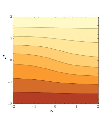
Figure 2. Level curves $L_{c}$ for $h=1$.

Since the “height” (in the $x_{2}$-direction) of $L_{c}$ is less than $h$ and $L_{c}$ is decreasing in the $x_{1}$-direction, we have that for any $c\in\mathbb{R}$, $L_{c}$ intersects (at most) only one horizontal line of the family $x_{2}=hz$, $z\in\mathbb{Z}$, and this intersection is given by a single point. From this, we deduce that the function $u:h\mathbb{Z}^{2}\to\mathbb{R}$ is injective. Thus, by denoting with $\mathrm{Im}(u)$ the image of $u$, there exists $u^{-1}:\mathrm{Im}(u)\to h\mathbb{Z}^{2}$ such that

(4.93) $$u^{-1}(u_{i})=i,\quad\text{for all }\,i\in h\mathbb{Z}^{2}.$$

Now we define $\hat{f}:\mathbb{R}\to\mathbb{R}$ as follows

$$\hat{f}(x)=\begin{cases}\tilde{f}\circ u^{-1}(x),&\quad\text{ for }\,x\in\mathrm{Im}(u),\\ 0,&\quad\text{ for }\,x\in\mathbb{R}\setminus\mathrm{Im}(u).\end{cases}$$

For all $i\in h\mathbb{Z}^{2}$ we have

$$\tilde{f}(i)=\tilde{f}\circ u^{-1}(u_{i})=\hat{f}(u_{i}),$$

and hence (4.32) holds true. By (4.31), $u$ satisfies (1.8) with

$$f(i,u_{i}):=\tilde{f}(i)=\hat{f}(u_{i}).$$

In particular, $u$ is solution of

$${\mathcal{L}}u_{i}=\hat{f}(u_{i}),$$

where the source term $\hat{f}$ only depends on $u$.

Example 4.3.

For any

(4.94) $$0<h\leqslant 1.$$

we consider

$$u_{i}:=i_{2}+\frac{h}{2}\,e^{-|i|^{2}}$$

and we define

$$\tilde{f}(i):=\mathcal{L}u_{i}=\frac{e^{-|i|^{2}}}{h}\,\sum_{j=1}^{2}\big{(}e^{-2hi_{j}-h^{2}}+e^{2hi_{j}-h^{2}}-2\big{)}$$

and

(4.95) $$f(i,u_{i}):=\tilde{f}(i).$$

In this way, we have that (1.8) holds true. Also, $f$ satisfies (1.11). Indeed, given $i\in h\mathbb{Z}^{2}$, we have that the map $\mathbb{R}\ni r\mapsto f(i,r)$ is constant, thus $f^{\prime}(i,\cdot)=0$. Additionally,

$$\big{|}e^{-2hi_{j}}+e^{2hi_{j}}-2\big{|} = \left|\sum_{k=0}^{+\infty}\frac{(-2hi_{j})^{k}}{k!}+\sum_{k=0}^{+\infty}\frac{(2hi_{j})^{k}}{k!}-2\right|$$

$$= \left|\sum_{k=2}^{+\infty}\frac{(-2hi_{j})^{k}}{k!}+\sum_{k=2}^{+\infty}\frac{(2hi_{j})^{k}}{k!}\right|$$

$$\leqslant 2\sum_{k=2}^{+\infty}\frac{(2h|i|)^{k}}{k!}$$

$$= 8h^{2}|i|^{2}\sum_{j=0}^{+\infty}\frac{(2h|i|)^{j}}{(j+2)!}$$

$$\leqslant 8h^{2}|i|^{2}\sum_{j=0}^{+\infty}\frac{(2h|i|)^{j}}{j!}$$

$$= 8h^{2}|i|^{2}e^{2h|i|}$$

$$\leqslant 8h^{2}|i|^{2}e^{2|i|}$$

and, as a result,

$$\big{|}e^{-2hi_{j}-h^{2}}+e^{2hi_{j}-h^{2}}-2\big{|}\leqslant\big{|}e^{-2hi_{j}-h^{2}}+e^{2hi_{j}-h^{2}}-2e^{-h^{2}}\big{|}+2(1-e^{-h^{2}})$$

$$\qquad\leqslant\big{|}e^{-2hi_{j}}+e^{2hi_{j}}-2\big{|}+2\left(1-\sum_{k=0}^{+\infty}\frac{(-h^{2})^{k}}{k!}\right)$$

$$\qquad\leqslant 8h^{2}|i|^{2}e^{2h|i|}-2\sum_{k=1}^{+\infty}\frac{(-h^{2})^{k}}{k!}$$

$$\qquad=8h^{2}|i|^{2}e^{2h|i|}+2h^{2}\sum_{j=0}^{+\infty}\frac{(-h^{2})^{j}}{(j+1)!}$$

$$\qquad\leqslant 8h^{2}|i|^{2}e^{2h|i|}+2h^{2}\sum_{j=0}^{+\infty}\frac{h^{2j}}{j!}$$

$$\qquad\leqslant 8h^{2}|i|^{2}e^{2h|i|}+2e^{h^{2}}h^{2}$$

$$\qquad\leqslant 8h^{2}\big{(}|i|^{2}e^{2h|i|}+1\big{)}.$$

Consequently,

$$|\nabla\tilde{f}(i)| \leqslant \frac{2|i|\,e^{-|i|^{2}}}{h}\,\sum_{j=1}^{2}\big{|}e^{-2hi_{j}-h^{2}}+e^{2hi_{j}-h^{2}}-2\big{|}+2e^{-|i|^{2}}\,\sum_{j=1}^{2}\big{|}e^{-2hi_{j}-h^{2}}-e^{2hi_{j}-h^{2}}\big{|}$$

$$\leqslant 32\,h\,|i|\,e^{-|i|^{2}}\big{(}|i|^{2}e^{2h|i|}+1\big{)}+2e^{-|i|^{2}}\,\sum_{j=1}^{2}\left|\int_{-2hi_{j}}^{2hi_{j}}e^{t}\,dt\right|$$

$$\leqslant 32\,h\,|i|\,e^{-|i|^{2}+2h|i|}\big{(}|i|^{2}+1\big{)}+16\,h\,|i|\,e^{-|i|^{2}+2h|i|}$$

$$\leqslant 32\,h\,|i|\,e^{-|i|^{2}+2|i|}\big{(}|i|^{2}+2\big{)}$$

$$\leqslant 32\,S\,h,$$

where

$$S:=\sup_{t\in\mathbb{R}}\Big{(}t\,e^{-t^{2}+2t}\big{(}t^{2}+2\big{)}\Big{)}.$$

Therefore, for all $i\in h\mathbb{Z}^{2}$,

$$\sum_{j=1}^{2}\frac{\big{|}f(i+he_{j},u_{i+he_{j}})-f(i,u_{i})-f^{\prime}(i,u_{i})(u_{i+he_{j}}-u_{i})\big{|}}{h}=\sum_{j=1}^{2}\frac{\big{|}\tilde{f}(i+he_{j})-\tilde{f}(i)\big{|}}{h}\leqslant\kappa_{0}^{+}\,h,$$

with $\kappa_{0}^{+}:=64\,S$, which yields (1.11).

In addition, for any $h>0$, $u$ is not one-dimensional, (4.16) holds true, and, if $h$ is small enough, then (1.10), (1.11), (1.14), (1.18), (1.21), and (1.35) (and hence (1.13)), are all satisfied. Thus, Theorem 1.1 applies, but $u$ is not one-dimensional. The computations to verify all the assumptions are similar to those of Example 4.2.

In the formal limit as $h\searrow 0$, an asymptotic analysis similar to that of Example 4.2 can be performed. As in Example 4.2, left-hand side and right-hand side of (1.22) are both of the order of $h^{2}$. Thus, also this example confirms the optimality of (1.22).

We conclude by showing that, also the function presented in this example can be seen as solution of an equation of the type

$${\mathcal{L}}u_{i}=\hat{f}(u_{i}),$$

where the source term $\hat{f}$ only depends on $u$.

For any $c\in\mathbb{R}$, the “height” (in the $x_{2}$-direction) of the level curve

$$L_{c}:=\left\{x_{2}+\frac{h}{2}\,e^{-(x_{1}^{2}+x_{2}^{2})}=c,\quad{\mbox{for}}\quad(x_{1},x_{2})\in\mathbb{R}^{2}\right\}$$

is less than $h/2$, whenever (4.94) is in force. Also, $L_{c}$ is symmetric with respect to the $x_{2}$-axis — i.e., $(x_{1},x_{2})\in L_{c}$ if and only if $(-x_{1},x_{2})\in L_{c}$ —, and it is increasing (resp. decreasing) in the $x_{1}$-direction for $x_{1}>0$ (resp. $x_{1}<0$). Thus, we have that for any $c\in\mathbb{R}$, $L_{c}$ intersects (at most) only one horizontal line of the family $x_{2}=hz$, $z\in\mathbb{Z}$, and this intersection is given by a single point

$$(\overline{x}_{1},\overline{x}_{2})\in\mathbb{R}^{+}\times\mathbb{R}:=\left\{(x_{1},x_{2})\in\mathbb{R}^{2}\,:\,x_{1}\geqslant 0\right\}$$

in the right half-space, and its symmetric

$$(-\overline{x}_{1},\overline{x}_{2})\in\mathbb{R}^{-}\times\mathbb{R}:=\left\{(x_{1},x_{2})\in\mathbb{R}^{2}\,:\,x_{1}\leqslant 0\right\}$$

in the left half-space. See Figure 3 for a sketch of the level curves $L_{c}$.

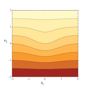
Figure 3. Level curves $L_{c}$ for $h=1$.

Hence, the function $u:h\mathbb{Z}^{2}\to\mathbb{R}$ is injective on $h\mathbb{Z}^{+}\times h\mathbb{Z}$ (or $h\mathbb{Z}^{-}\times h\mathbb{Z}$), where $h\mathbb{Z}^{+}\times h\mathbb{Z}$ (resp. $h\mathbb{Z}^{-}\times h\mathbb{Z}$) is the set of points $i=(i_{1},i_{2})\in h\mathbb{Z}^{2}$ such that $i_{1}\geqslant 0$ (resp. $i_{1}\leqslant 0$).

Thus, by denoting with $\mathrm{Im}(u)$ the image of $u$, there exists $u^{-1}:\mathrm{Im}(u)\to h\mathbb{Z}^{+}\times h\mathbb{Z}$ such that

$$u^{-1}(u_{i})=i,\quad\text{ for all }i\in h\mathbb{Z}^{+}\times h\mathbb{Z}.$$

Now we define $\hat{f}:\mathbb{R}\to\mathbb{R}$ as follows

$$\hat{f}(x)=\begin{cases}\tilde{f}\circ u^{-1}(x)&\quad\text{ for }\,x\in\mathrm{Im}(u),\\ 0&\quad\text{ for }\,x\in\mathbb{R}\setminus\mathrm{Im}(u),\end{cases}$$

and we notice that

$$\tilde{f}(i)=\tilde{f}\circ u^{-1}(u_{i})=\hat{f}(u_{i}),\quad\text{ for all }\,i\in h\mathbb{Z}^{2}.$$

The previous identity clearly holds true, by definition of $\hat{f}$, whenever $i\in h\mathbb{Z}^{+}\times h\mathbb{Z}$. However, it remains true even if $i\in h\mathbb{Z}^{-}\times h\mathbb{Z}$. Indeed, thanks to the symmetry properties

$$u_{(i_{1},i_{2})}=u_{(-i_{1},i_{2})}\quad\text{ for any }i=(i_{1},i_{2})\in h\mathbb{Z}^{2},$$

$$\tilde{f}(i_{1},i_{2})=\tilde{f}(-i_{1},i_{2})\quad\text{ for any }i=(i_{1},i_{2})\in h\mathbb{Z}^{2},$$

if $i=(i_{1},i_{2})\in h\mathbb{Z}^{-}\times h\mathbb{Z}$ we can still write

$$\tilde{f}(i)=\tilde{f}(i_{1},i_{2})=\tilde{f}(-i_{1},i_{2})=\tilde{f}\circ u^{-1}(u_{(-i_{1},i_{2})})=\hat{f}(u_{(-i_{1},i_{2})})=\hat{f}(u_{(i_{1},i_{2})})=\hat{f}(u_{i}).$$

Thus, for any $i\in h\mathbb{Z}^{2}$ (1.8) holds true with

$$f(i,u_{i}):=\tilde{f}(i)=\hat{f}(u_{i}).$$

In particular, by (4.95), $u$ is solution of

$${\mathcal{L}}u_{i}=\hat{f}(u_{i}),$$

where the source term $\hat{f}$ only depends on $u$.

The previous three examples have been obtained by perturbing the one-dimensional linear function $i_{2}$. We stress that more general examples could be obtained by perturbing different one-dimensional functions. For instance, the following example is obtained by perturbing a (strictly monotone) one-dimensional solution $\tilde{v}:\mathbb{R}\to\mathbb{R}$ of a general semilinear autonomous equation $\tilde{v}^{\prime\prime}=g(\tilde{v})$, with the perturbation already used in Example 4.1. As a concrete reference case, one may think to, e.g., $\tilde{v}(t):=4\arctan(e^{t})$ which satisfies the stationary sine-Gordon equation

(4.96) $$\tilde{v}^{\prime\prime}=\sin\left(\tilde{v}\right).$$

Of course, Example 4.1 is a particular case of Example 4.4 (in which $\tilde{v}(t):=t$ and $g\equiv 0$).

Example 4.4.

Consider $\tilde{v}:\mathbb{R}\to\mathbb{R}$ satisfying the semilinear equation

(4.97) $$\tilde{v}^{\prime\prime}=g(\tilde{v}),$$

where $g:\mathbb{R}\to\mathbb{R}$. For $x=(x_{1},x_{2})\in\mathbb{R}^{2}$ we set

(4.98) $$\overline{v}(x):=\tilde{v}(x_{2}),$$

and for $i=(i_{1},i_{2})$ we define

(4.99) $$v_{i}:=\overline{v}(i),$$

which is the restriction of $\overline{v}$ to $h\mathbb{Z}^{2}$. With these definitions we clearly have

$$\Delta\overline{v}(x)=\tilde{v}^{\prime\prime}(x_{2}),\quad{\mbox{ for all }}x\in\mathbb{R}^{2},$$

and $${\mathcal{L}}v_{i}={\mathcal{L}}_{2}v_{i},\quad{\mbox{ for all }}i\in\mathbb{R}^{2},$$

where we have used the notation in (1.19) for ${\mathcal{L}}_{2}$.

We now show that, if $\|\tilde{v}^{\prime}\|_{L^{\infty}(\mathbb{R})}<\infty$, $\|\tilde{v}^{(iv)}\|_{L^{\infty}(\mathbb{R})}<\infty$ and $\|g^{\prime\prime}\|_{L^{\infty}(\mathbb{R})}<\infty$, then $v$, as defined in (4.99), satisfies assumption (1.9) with $f(i,u_{i})$ and $L_{f}^{+}(i,u_{i})$ replaced by ${\mathcal{L}}v_{i}$ and $g^{\prime}(v_{i})$. Here, $\tilde{v}^{(iv)}$ denotes the fourth derivative of $\tilde{v}$.

Indeed, a fourth order Taylor expansion with Lagrange remainder terms shows that

(4.100) $$\begin{split}&\frac{\left({\mathcal{L}}v\right)_{i+he_{2}}+\left({\mathcal{L}}v\right)_{i}-g^{\prime}(v_{i})(v_{i+he_{2}}-v_{i})}{h}\\ &\qquad=\,\frac{h}{4!}\left[\sum_{k=1}^{4}\tilde{v}^{(iv)}(i+\xi_{k}e_{2})\right]+\frac{\tilde{v}^{\prime\prime}(i+he_{2})-\tilde{v}^{\prime\prime}(i)-g^{\prime}(v_{i})(v_{i+he_{2}}-v_{i})}{h}\end{split}$$

for some $\xi_{1}$, $\xi_{4}\in(0,h)$, $\xi_{2}\in(0,-h)$, $\xi_{3}\in(h,2h)$. By using (4.97) we compute

(4.101) $$\begin{split}\frac{\tilde{v}^{\prime\prime}(i+he_{2})-\tilde{v}^{\prime\prime}(i)-g^{\prime}(v_{i})(v_{i+he_{2}}-v_{i})}{h}=&\,\frac{g(i+he_{2})-g(i)-g^{\prime}(v_{i})(v_{i+he_{2}}-v_{i})}{h}\\ =&\,\frac{g^{\prime\prime}(v_{i}+\eta)}{2}\,\left[\frac{v_{i+he_{2}}-v_{i}}{h}\right]^{2}\,h\\ =&\,\frac{g^{\prime\prime}(v_{i}+\eta)}{2}\,\left[v^{\prime}(i+\xi_{5})\right]^{2}\,h,\end{split}$$

for some $\eta\in(0,v_{i+he_{2}}-v_{i})$, $\xi_{5}\in(0,h)$. By using that $v$ only depends on $i_{2}$ and putting together (4.100) and (4.101) we get that

(4.102) $$\begin{split}\sum_{j=1}^{2}\frac{\left({\mathcal{L}}v\right)_{i+he_{j}}+\left({\mathcal{L}}v\right)_{i}-g^{\prime}(v_{i})(v_{i+he_{j}}-v_{i})}{h}=&\,\frac{\left({\mathcal{L}}v\right)_{i+he_{2}}+\left({\mathcal{L}}v\right)_{i}-g^{\prime}(v_{i})(v_{i+he_{2}}-v_{i})}{h}\\ \leqslant&\,h\left\{\frac{\|\tilde{v}^{(iv)}\|_{L^{\infty}(\mathbb{R})}}{6}+\frac{\|g^{\prime\prime}\|_{L^{\infty}(\mathbb{R})}}{2}\|\tilde{v}^{\prime}\|_{L^{\infty}(\mathbb{R})}\right\},\end{split}$$

that is, $v$ satisfies (1.9) — where $f(i,u_{i})$ and $L_{f}^{+}(i,u_{i})$ are replaced by ${\mathcal{L}}v_{i}$ and $g^{\prime}(v_{i})$ — with

$$k_{0}^{+}=\frac{\|\tilde{v}^{(iv)}\|_{L^{\infty}(\mathbb{R})}}{6}+\frac{\|g^{\prime\prime}\|_{L^{\infty}(\mathbb{R})}}{2}\|\tilde{v}^{\prime}\|_{L^{\infty}(\mathbb{R})}.$$

Notice that in concrete cases in which $\tilde{v}$ and $g$ are explicitly given, one could explicitly compute $\|\tilde{v}^{\prime}\|_{L^{\infty}(\mathbb{R})}$, $\|\tilde{v}^{(iv)}\|_{L^{\infty}(\mathbb{R})}$ and $\|g^{\prime\prime}\|_{L^{\infty}(\mathbb{R})}$.

We now denote by $w$ the perturbation already used in Example 4.1, that is,

(4.103) $$w_{i}:=\begin{cases}h^{4}\quad&\text{for }\,i=(i_{1},0),\,i_{1}>0,\\ 0\quad\,&\text{otherwise in }h\mathbb{Z}^{2}.\end{cases}$$

For any

(4.104) $$0<h<1$$

and $i=(i_{1},i_{2})\in h\mathbb{Z}^{2}$, we then consider

(4.105) $$u_{i}:=v_{i}+w_{i}$$

and we set

(4.106) $$f(i,u_{i}):=\tilde{f}(i):={\mathcal{L}}v_{i}+{\mathcal{L}}w_{i},$$

so that ${\mathcal{L}}u_{i}=\tilde{f}(i)$, and therefore (1.8) is satisfied.

We now show that, if $\|\tilde{v}^{\prime}\|_{L^{\infty}(\mathbb{R})}<\infty$, $\|\tilde{v}^{(iv)}\|_{L^{\infty}(\mathbb{R})}<\infty$, $\|g^{\prime}\|_{L^{\infty}(\mathbb{R})}<\infty$ and $\|g^{\prime\prime}\|_{L^{\infty}(\mathbb{R})}<\infty$, then $f$ satisfies (1.9) with $L_{f}^{+}(i,u_{i}):=g^{\prime}(v_{i})$.

To check this, we start by computing

(4.107) $$\begin{split}&\sum_{j=1}^{2}\frac{\left|\tilde{f}(i+he_{j})-\tilde{f}(i)-g^{\prime}(v_{i})(u_{i+he_{j}}-u_{i})\right|}{h}\\ &=\,\sum_{j=1}^{2}\frac{\left|\left({\mathcal{L}}v\right)_{i+he_{j}}+\left({\mathcal{L}}w\right)_{i+he_{j}}-\left({\mathcal{L}}v\right)_{i}-\left({\mathcal{L}}w\right)_{i}-g^{\prime}(v_{i})(v_{i+he_{j}}+w_{i+he_{j}}-v_{i}-w_{i})\right|}{h}\\ &\leqslant\,\left\{\sum_{j=1}^{2}\frac{\left|\left({\mathcal{L}}v\right)_{i+he_{j}}-\left({\mathcal{L}}v\right)_{i}-g^{\prime}(v_{i})(v_{i+he_{j}}-v_{i})\right|}{h}\right\}+\left\{\sum_{j=1}^{2}\frac{\left|\left({\mathcal{L}}w\right)_{i+he_{j}}-\left({\mathcal{L}}w\right)_{i}-g^{\prime}(v_{i})(w_{i+he_{j}}-w_{i})\right|}{h}\right\}.\end{split}$$

Here, in the last inequality we used the triangle inequality.

The term in the first braces in (4.107) can be estimated by means of (4.102). We now estimate the term in the second braces as follows:

(4.108) $$\begin{split}\sum_{j=1}^{2}&\frac{\left|\left({\mathcal{L}}w\right)_{i+he_{j}}-\left({\mathcal{L}}w\right)_{i}-g^{\prime}(v_{i})(w_{i+he_{j}}-w_{i})\right|}{h}\\ \leqslant&\sum_{j=1}^{2}\frac{\left|\left({\mathcal{L}}w\right)_{i+he_{j}}-\left({\mathcal{L}}w\right)_{i}\right|}{h}+\|g^{\prime}\|_{L^{\infty}(\mathbb{R})}\frac{\left|w_{i+he_{j}}-w_{i}\right|}{h}\\ \leqslant&\,\sum_{j=1}^{2}\frac{\left|\left({\mathcal{L}}w\right)_{i+he_{j}}-\left({\mathcal{L}}w\right)_{i}\right|}{h}+\|g^{\prime}\|_{L^{\infty}(\mathbb{R})}\,h^{3}\\ \leqslant&\,\sum_{j=1}^{2}\frac{\left|\left({\mathcal{L}}w\right)_{i+he_{j}}-\left({\mathcal{L}}w\right)_{i}\right|}{h}+\|g^{\prime}\|_{L^{\infty}(\mathbb{R})}\,h\end{split}.$$

Here, the first inequality follows by the triangle inequality, the second inequality can be deduced by (4.103), and the third inequality follows by (4.104).

By noting that ${\mathcal{L}}w_{i}$ coincides with the function $\tilde{f}(i)$ defined in (4.2) (in Example 4.1), the same computations that gave (4.3) now inform us that

(4.109) $$\sum_{j=1}^{2}\frac{\left|\left({\mathcal{L}}w\right)_{i+he_{j}}-\left({\mathcal{L}}w\right)_{i}\right|}{h}\leqslant 5\,h.$$

By putting together (4.107), (4.102), (4.108) and (4.109), we thus obtain that $f$ (as defined in (4.106)) satisfies (1.11) with $L_{f}^{+}(i,u_{i})=g^{\prime}(v_{i})$ and

(4.110) $$\kappa_{0}^{+}=\left\{\frac{\|\tilde{v}^{(iv)}\|_{L^{\infty}(\mathbb{R})}}{6}+\frac{\|g^{\prime\prime}\|_{L^{\infty}(\mathbb{R})}}{2}\|\tilde{v}^{\prime}\|_{L^{\infty}(\mathbb{R})}\right\}+\left\{5+\|g^{\prime}\|_{L^{\infty}(\mathbb{R})}\right\}.$$

From now on we assume that $\tilde{v}$ is strictly increasing (this is indeed the case of the sine-Gordon equation). Under this assumption it is clear that, if $h$ is small enough, then $u$ satisfies (1.35), and hence (1.13) holds true. In fact, by recalling the definition of $u$ in (4.105), we have that $u$ satisfies (1.35) if and only if

$$v_{(h,h)}-v_{(h,0)}>h^{4}$$

and hence — by recalling that $v_{(h,h)}=v_{(0,h)}$ and $v_{(h,0)}=v_{(0,0)}$ (since $v$ depends on $i_{2}$ only) — if and only if

$$\mathcal{D}_{2}^{+}v_{(0,0)}>h^{3}.$$

For this reason and recalling (4.104), from now on we assume

(4.111) $$0<h<\min\left\{1,\left(\mathcal{D}_{2}^{+}v_{(0,0)}\right)^{1/3}\right\}$$

We stress that $\mathcal{D}_{2}^{+}v_{(0,0)}$ is always a number strictly greater than $0$ in light of the assumption that $\tilde{v}$ is strictly increasing. Moreover, ${\mathcal{D}}_{2}^{+}v_{(0,0)}$ could be explicitly computed in concrete examples in which $\tilde{v}$ is explicitly given.

We now show that $u$ also satisfies (1.14), (1.18) and (1.21) with $\vartheta^{+}_{\infty}:=\pi/2$. To this aim, we directly compute

$${\mathcal{D}}_{1}^{+}u_{i}=\begin{cases}h^{3}\quad\,&\text{for }\,i=(0,0),\\ 0\quad\,&\text{otherwise in }\,h\mathbb{Z}^{2},\end{cases}\qquad\text{ and }\qquad{\mathcal{D}}_{2}^{+}u_{i}=\begin{cases}{\mathcal{D}}_{2}^{+}v_{i}-h^{3}\quad\,&\text{for }\,i=(i_{1},0)\text{ with }i_{1}>0,\\ {\mathcal{D}}_{2}^{+}v_{i}+h^{3}\quad\,&\text{for }\,i=(i_{1},-h)\text{ with }i_{1}>0,\\ 1\quad\,&\text{otherwise in }\,h\mathbb{Z}^{2},\end{cases}$$

and hence

$$\vartheta^{+}_{i} = \begin{cases}\arctan\left(\frac{{\mathcal{D}}_{2}^{+}v_{i}}{h^{3}}\right)\quad\,&\text{for }\,i=(0,0),\\ \frac{\pi}{2}\quad&\text{otherwise in }\,h\mathbb{Z}^{2},\end{cases}$$

$$\text{and }\qquad(\rho_{i}^{+})^{2} = \begin{cases}\left({\mathcal{D}}_{2}^{+}v_{i}\right)^{2}+h^{6}\quad\,&\text{for }\,i=(0,0),\\ ({\mathcal{D}}_{2}^{+}v_{i}-h^{3})^{2}\quad\,&\text{for }\,i=(i_{1},0)\,\text{ with }\,i_{1}>0,\\ ({\mathcal{D}}_{2}^{+}v_{i}+h^{3})^{2}\quad\,&\text{for }\,i=(i_{1},-h)\,\text{ with }\,i_{1}>0,\\ \left({\mathcal{D}}_{2}^{+}v_{i}\right)^{2}\quad&\text{otherwise in }\,h\mathbb{Z}^{2}.\end{cases}$$

By recalling (4.25) and (4.98) we get that

$$|{\mathcal{D}}_{2}^{+}v_{i}|\leqslant\|\tilde{v}^{\prime}\|_{L^{\infty}(\mathbb{R})},$$

and hence, by recalling that $0<h<1$, we find that

(4.112) $$\rho_{i}^{+}\leqslant\|\tilde{v}^{\prime}\|_{L^{\infty}(\mathbb{R})}+h^{3}<\|\tilde{v}^{\prime}\|_{L^{\infty}(\mathbb{R})}+1=:S.$$

We also notice that

$$\kappa_{1}^{+}:=\sup_{{1\leqslant j\leqslant 2}\atop{i\in h\mathbb{Z}^{2}}}|{\mathcal{D}}_{j}^{+}u_{i}|\leqslant\|\tilde{v}^{\prime}\|_{L^{\infty}(\mathbb{R})}+h^{3}<\|\tilde{v}^{\prime}\|_{L^{\infty}(\mathbb{R})}+1=S,$$

being $0<h<1$, and this establishes (1.14).

We then compute

$${\mathcal{D}}_{1}^{+}\vartheta^{+}_{i}=\begin{cases}\frac{1}{h}\left(\frac{\pi}{2}-\arctan\left(\frac{{\mathcal{D}}_{2}^{+}v_{(0,0)}}{h^{3}}\right)\right)\quad\,&\text{for }\,i=(0,0),\\ \frac{1}{h}\left(\arctan\left(\frac{{\mathcal{D}}_{2}^{+}v_{(0,0)}}{h^{3}}\right)-\frac{\pi}{2}\right)\quad\,&\text{for }\,i=(-h,0),\\ 0\quad\,&\text{otherwise in }\,h\mathbb{Z}^{2},\end{cases}$$

$${\mathcal{D}}_{2}^{+}\vartheta^{+}_{i}=\begin{cases}\frac{1}{h}\left(\frac{\pi}{2}-\arctan\left(\frac{{\mathcal{D}}_{2}^{+}v_{(0,0)}}{h^{3}}\right)\right)\quad\,&\text{for }\,i=(0,0),\\ \frac{1}{h}\left(\arctan\left(\frac{{\mathcal{D}}_{2}^{+}v_{(0,0)}}{h^{3}}\right)-\frac{\pi}{2}\right)\quad\,&\text{for }\,i=(0,-h),\\ 0\quad\,&\text{otherwise in }\,h\mathbb{Z}^{2},\end{cases}$$

$${\mathcal{D}}_{1}^{+}\left({\mathcal{D}}_{1}^{+}\vartheta^{+}\right)_{i-he_{j}}=\begin{cases}\frac{2}{h^{2}}\left(\frac{\pi}{2}-\arctan\left(\frac{{\mathcal{D}}_{2}^{+}v_{(0,0)}}{h^{3}}\right)\right)\quad\,&\text{for }\,i=(0,0),\\ \frac{1}{h^{2}}\left(\arctan\left(\frac{{\mathcal{D}}_{2}^{+}v_{(0,0)}}{h^{3}}\right)-\frac{\pi}{2}\right)\quad\,&\text{for }\,i=(\pm h,0),\\ 0\quad\,&\text{otherwise in }\,h\mathbb{Z}^{2},\end{cases}$$

and

$${\mathcal{D}}_{2}^{+}\left({\mathcal{D}}_{2}^{+}\vartheta^{+}\right)_{i-he_{j}}=\begin{cases}\frac{2}{h^{2}}\left(\frac{\pi}{2}-\arctan\left(\frac{{\mathcal{D}}_{2}^{+}v_{(0,0)}}{h^{3}}\right)\right)\quad\,&\text{for }\,i=(0,0),\\ \frac{1}{h^{2}}\left(\arctan\left(\frac{{\mathcal{D}}_{2}^{+}v_{(0,0)}}{h^{3}}\right)-\frac{\pi}{2}\right)\quad\,&\text{for }\,i=(0,\pm h),\\ 0\quad\,&\text{otherwise in }\,h\mathbb{Z}^{2}.\end{cases}$$

By using (4.112) and recalling that the relations in (4.4) hold true for $\vartheta^{+}$, we can now directly compute

(4.113) $$\begin{split}\kappa_{2}^{+}=\,&\sum_{{1\leqslant j\leqslant 2}\atop{i\in h\mathbb{Z}^{2}}}\left(\rho_{i}^{+}\right)^{2}\Big{(}|{\mathcal{D}}_{j}^{+}\vartheta^{+}_{i}|\,|{\mathcal{D}}_{j}^{+}({\mathcal{D}}_{j}^{+}\vartheta^{+})_{i-he_{j}}|+|{\mathcal{D}}_{j}^{-}\vartheta^{+}_{i}|\,|{\mathcal{D}}_{j}^{-}({\mathcal{D}}_{j}^{-}\vartheta^{+})_{i+he_{j}}|\Big{)}\\ \leqslant\,&12\,S^{2}\,\frac{\left(\frac{\pi}{2}-\arctan\left(\frac{{\mathcal{D}}_{2}^{+}v_{(0,0)}}{h^{3}}\right)\right)^{2}}{h^{3}},\end{split}$$

where $S$ is defined in (4.112). By using (4.6) with $t={\mathcal{D}}_{2}^{+}v_{(0,0)}/h^{3}$,

(4.114) $$\left|\mathrm{sgn}\left(\frac{{\mathcal{D}}_{2}^{+}v_{(0,0)}}{h^{3}}\right)\frac{\pi}{2}-\arctan\left(\frac{{\mathcal{D}}_{2}^{+}v_{(0,0)}}{h^{3}}\right)\right|\leqslant\frac{h^{3}}{{\mathcal{D}}_{2}^{+}v_{(0,0)}}.$$

From this and (4.113), we obtain that

(4.115) $$\kappa_{2}^{+}\leqslant 12\left(\frac{S}{{\mathcal{D}}_{2}^{+}v_{(0,0)}}\right)^{2}\,h^{3},$$

that gives (1.18) and also keeps track of the order of $h$.

In order to verify (1.21), we notice that, being $\vartheta_{\infty}^{+}=\pi/{2}$, we have that

$$|\vartheta_{i}^{+}-\vartheta_{\infty}^{+}|=\begin{cases}\frac{\pi}{2}-\arctan\left(\frac{{\mathcal{D}}_{2}^{+}v_{(0,0)}}{h^{3}}\right)\quad\,&\text{for }\,i=(0,0),\\ 0\quad\,&\text{otherwise in }\,h\mathbb{Z}^{2}.\end{cases}$$

Thus, the only nonzero term in the summations defining $\kappa_{3}^{+}$, $\kappa_{4}^{+}$, $\kappa_{5}^{+}$, $\kappa_{6}^{+}$, $\kappa_{7}^{+}$ in (1.21) are those for $i=(0,0)$.

We start by computing that

$$\kappa_{3}^{+}=4\left[\left({\mathcal{D}}_{2}^{+}v_{(0,0)}\right)^{2}+h^{6}\right]\frac{\left(\frac{\pi}{2}-\arctan\left(\frac{{\mathcal{D}}_{2}^{+}v_{(0,0)}}{h^{3}}\right)\right)^{4}}{h^{3}},$$

which, in light of (4.114), gives that

$$\kappa_{3}^{+}\leqslant\frac{4}{\left({\mathcal{D}}_{2}^{+}v_{(0,0)}\right)^{2}}\left[1+\left(\frac{h^{3}}{{\mathcal{D}}_{2}^{+}v_{(0,0)}}\right)^{2}\right]\,h^{9}$$

and hence, by recalling (4.111), that

(4.116) $$\kappa_{3}^{+}\leqslant\frac{8}{\left({\mathcal{D}}_{2}^{+}v_{(0,0)}\right)^{2}}\,h^{9}.$$

In order to estimate $\kappa_{4}^{+}$, $\kappa_{6}^{+}$, $\kappa_{7}^{+}$ we just need to compute

$$\mathcal{L}_{1}^{2}\vartheta_{(0,0)}^{+}=\mathcal{L}_{2}^{2}\vartheta_{(0,0)}^{+}=\frac{6}{h^{4}}\left(\arctan\left(\frac{{\mathcal{D}}_{2}^{+}v_{(0,0)}}{h^{3}}\right)-\frac{\pi}{2}\right),$$

and to notice that, by (4.112), we have that

(4.117) $$|{\mathcal{D}}_{j}^{\pm}\rho_{(0,0)}^{+}|\leqslant\frac{2\,S}{h},\quad{\mbox{ for }}j=1,2,$$

and

(4.118) $$|{\mathcal{D}}_{j}^{\pm}\left(\rho_{(0,0)}^{+}\right)^{2}|\leqslant\frac{2\,S^{2}}{h},\quad{\mbox{ for }}j=1,2.$$

We stress that more accurate computations (similar to those performed in Example 4.1) could be performed in order to obtain the exact values of $|{\mathcal{D}}_{j}^{\pm}\rho_{(0,0)}^{+}|$ and $\Big{|}{\mathcal{D}}_{j}^{\pm}\left(\rho_{(0,0)}^{+}\right)^{2}\Big{|}$. However, the bounds in (4.117) and (4.118) are sufficient in order to verify that $u$ satisfies (1.21) and also to check the optimality of Theorem 1.1.

By putting together that

$$\rho^{+}_{(0,0)}=\sqrt{\left({\mathcal{D}}_{2}^{+}v_{(0,0)}\right)^{2}+h^{6}}={\mathcal{D}}_{2}^{+}v_{(0,0)}\,\sqrt{1+\left(\frac{h^{3}}{{\mathcal{D}}_{2}^{+}v_{(0,0)}}\right)^{2}}$$

and (4.111), we obtain that

(4.119) $$\rho^{+}_{(0,0)}\leqslant\sqrt{2}\ {\mathcal{D}}_{2}^{+}v_{(0,0)}.$$

By using (4.117) and (4.119), we now compute that

$$\kappa_{4}^{+}\leqslant\left(\sqrt{2}\ {\mathcal{D}}_{2}^{+}v_{(0,0)}\right)\,\left(\frac{2\,S}{h}\right)\,4\,\frac{\left(\frac{\pi}{2}-\arctan\left(\frac{{\mathcal{D}}_{2}^{+}v_{(0,0)}}{h^{3}}\right)\right)^{3}}{h^{2}}.$$

From this and (4.114), we deduce that

(4.120) $$\kappa_{4}^{+}\leqslant 8\sqrt{2}\,\frac{S}{\left({\mathcal{D}}_{2}^{+}v_{(0,0)}\right)^{2}}\,h^{6}.$$

By using (4.119), we also find that

$$\kappa_{5}^{+}\leqslant\kappa_{0}^{+}\,\sqrt{2}\ {\mathcal{D}}_{2}^{+}v_{(0,0)}\,\left(\frac{\pi}{2}-\arctan\left(\frac{1}{h^{3}}\right)\right),$$

where $\kappa_{0}^{+}$ is that obtained in (4.110). Thus, by (4.114), we see that

(4.121) $$\kappa_{5}^{+}\leqslant\kappa_{0}^{+}\sqrt{2}\ h^{3}.$$

By using the inequality $\left(\rho^{+}_{(0,0)}\right)^{2}\leqslant 2\left({\mathcal{D}}_{2}^{+}v_{(0,0)}\right)^{2}$ — which follows by (4.119) — and (4.118), we then compute

$$\kappa_{6}^{+}\leqslant\left[\left(\frac{2\,S^{2}}{h}\right)\,4\,\frac{\left(\frac{\pi}{2}-\arctan\left(\frac{{\mathcal{D}}_{2}^{+}v_{(0,0)}}{h^{3}}\right)\right)}{h}+24\left({\mathcal{D}}_{2}^{+}v_{(0,0)}\right)^{2}\,\frac{\left(\frac{\pi}{2}-\arctan\left(\frac{{\mathcal{D}}_{2}^{+}v_{(0,0)}}{h^{3}}\right)\right)}{h^{3}}\right]\left(\frac{\pi}{2}-\arctan\left(\frac{{\mathcal{D}}_{2}^{+}v_{(0,0)}}{h^{3}}\right)\right),$$

and hence, by (4.114),

(4.122) $$\kappa_{6}^{+}\leqslant\left[\frac{8\,S^{2}}{\left({\mathcal{D}}_{2}^{+}v_{(0,0)}\right)^{2}}\,h+24\right]\,h^{3}.$$

Finally, by using (4.117) we find that

$$\kappa_{7}^{+}\leqslant\left(\frac{2\,S}{h}\right)^{2}\left[4\,\frac{\left(\frac{\pi}{2}-\arctan\left(\frac{{\mathcal{D}}_{2}^{+}v_{(0,0)}}{h^{3}}\right)\right)}{h}\right]\,\left(\frac{\pi}{2}-\arctan\left(\frac{{\mathcal{D}}_{2}^{+}v_{(0,0)}}{h^{3}}\right)\right),$$

and hence, by (4.114), we obtain that

(4.123) $$\kappa_{7}^{+}\leqslant\left[\frac{16\,S^{2}}{\left({\mathcal{D}}_{2}^{+}v_{(0,0)}\right)^{2}}\right]\,h^{3}.$$

In light of (4.104), inequalities (4.116), (4.120), (4.121), (4.122) and (4.123) give (1.21).

All in all, we have that $u$ and $f$ satisfy all the assumptions of Theorem 1.1 and hence (1.22) holds true. Nevertheless $u$ is not one-dimensional, and (4.16) holds true.

We notice that the quantity in the left-hand side of (4.16) can be explicitly computed. Here, as usual, in order to check the optimality of Theorem 1.1, we just notice that

$$\sum\limits_{{1\leqslant j\leqslant 2}\atop{i\in h\mathbb{Z}^{2}}}(\rho_{i}^{+})^{2}\;\Big{(}|{\mathcal{D}}_{j}^{+}\vartheta^{+}_{i}|^{2}+|{\mathcal{D}}_{j}^{-}\vartheta^{+}_{i}|^{2}\Big{)} \geqslant (\rho_{(-h,0)}^{+})^{2}\;\sum\limits_{j=1}^{2}\Big{(}|{\mathcal{D}}_{j}^{+}\vartheta^{+}_{(-h,0)}|^{2}+|{\mathcal{D}}_{j}^{-}\vartheta^{+}_{(-h,0)}|^{2}\Big{)}$$

$$= |{\mathcal{D}}_{2}^{+}v_{(-h,0)}|^{2}|{\mathcal{D}}_{1}^{+}\vartheta^{+}_{(-h,0)}|^{2}=|{\mathcal{D}}_{2}^{+}v_{(0,0)}|^{2}\frac{\left(\frac{\pi}{2}-\arctan\left(\frac{{\mathcal{D}}_{2}^{+}v_{(0,0)}}{h^{3}}\right)\right)^{2}}{h^{2}}.$$

Here, in the last equality we used the explicit value of ${\mathcal{D}}_{1}^{+}\vartheta^{+}_{(-h,0)}$ computed before, and the equality ${\mathcal{D}}_{2}^{+}v_{(0,0)}={\mathcal{D}}_{2}^{+}v_{(-h,0)}$ which holds true since $v$ is a function depending on the $i_{2}$-variable only.

By recalling (4.111), we can take $t={\mathcal{D}}_{2}^{+}v_{(0,0)}/h^{3}$ in (4.17), obtaining that

$$\left|\mathrm{sgn}\left(\frac{{\mathcal{D}}_{2}^{+}v_{(0,0)}}{h^{3}}\right)\frac{\pi}{2}-\arctan\left(\frac{{\mathcal{D}}_{2}^{+}v_{(0,0)}}{h^{3}}\right)\right|\geqslant\frac{4}{\pi}\,\frac{\left|h\right|^{3}}{{\mathcal{D}}_{2}^{+}v_{(0,0)}}.$$

From this we thus get that

(4.124) $$\sum\limits_{{1\leqslant j\leqslant 2}\atop{i\in h\mathbb{Z}^{2}}}(\rho_{i}^{+})^{2}\;\Big{(}|{\mathcal{D}}_{j}^{+}\vartheta^{+}_{i}|^{2}+|{\mathcal{D}}_{j}^{-}\vartheta^{+}_{i}|^{2}\Big{)}\geqslant\frac{4^{2}}{\pi^{2}}\,h^{4}.$$

On the other hand, (4.115), (4.116), (4.120), (4.121), (4.122), (4.123) and (4.104) give that the right-hand side of (1.22) satisfies

(4.125) $$C\,h\leqslant c_{1}h^{4},$$

where $C$ is the quantity defined in (1.23), and

$$c_{1}:=4\left\{\frac{1}{\left({\mathcal{D}}_{2}^{+}v_{(0,0)}\right)^{2}}\left[36\,S^{2}+16\,e^{2\pi}\left(1+\sqrt{2}\,S\right)\right]+2\sqrt{2}\,\kappa_{0}^{+}+24\right\},$$

where $\kappa_{0}^{+}$ and $S$ are those defined in (4.110) and (4.112).

Thus, by putting together (1.22), (4.124) and (4.125), it is clear that, in the formal limit as $h\searrow 0$, the left-hand side and the right-hand side of (1.22) are both of the order of $h^{4}$. Thus, also this general example confirms the optimality of (1.22).

We stress that $c_{1}$ is a positive constant only depending on (a lower bound on) ${\mathcal{D}}_{2}^{+}v_{(0,0)}$ and (upper bounds on) $\|\tilde{v}^{\prime}\|_{L^{\infty}(\mathbb{R})}$, $\|\tilde{v}^{(iv)}\|_{L^{\infty}(\mathbb{R})}$, $\|g^{\prime}\|_{L^{\infty}(\mathbb{R})}$, and $\|g^{\prime\prime}\|_{L^{\infty}(\mathbb{R})}$. We recall that, in concrete examples — such as, e.g., in the case of the sine-Gordon equation (4.96) —, these bounds can be explicitly obtained and $c_{1}$ is just a universal constant.

Appendix A The identity in (1.33) as a formal limit of the one in (1.31)

In this appendix, we discuss, merely at a formal level, how the continuous identity in (1.33) may be understood as a suitable limit of the discrete identity in (1.31) (and we believe that this observation is interesting, since it relates the identity in (1.33), which is classical and well understood, with the one in (1.31), which is, as far as we can tell, completely new in the literature).

Establishing a rigorous framework to relate (1.31) and (1.33) goes beyond the goals of this paper and would rather fit into the more comprehensive and ambitious goal of scrupulously connect discrete and continuous models, hence our arguments will rely on formal, yet solid, approximations. To deduce (1.33) from (1.31) we fix $(x_{1},x_{2})\in\mathbb{R}^{2}$. Without loss of generality, we suppose that $x_{1}>0$. Given $h>0$, we take $k\in\mathbb{N}$ such as $hk$ is as close as possible to $x_{1}$, for instance by taking $k$ such that $hk\leqslant x_{1}<h(k+1)$. Similarly, we take $m\in\mathbb{Z}$ such that $hm\leqslant x_{2}<h(m+1)$. As a matter of fact, to make the computation as transparent as possible, we simply suppose that $x_{1}=1$ and $x_{2}=0$, and also that $\frac{1}{h}\in\mathbb{N}$, in which case we have that $k=\frac{1}{h}$ and $m=0$. In this way, we can write (1.31) in the simpler form

(A.1) $$u_{(1,0)}=\sum_{j=0}^{1/h}{\binom{1/h}{j}}c^{j}\,(1-c)^{\frac{1}{h}-j}\,\widetilde{u}_{hj},$$

where $c$ is short for $c^{+}$. Similarly, we can state (1.33) in its simpler version given by

(A.2) $$u(1,0)=\widetilde{u}(c).$$

Since the role of the point $(x_{1},x_{2})=(1,0)$ is somehow arbitrary, we focus on the relation between (A.1) and (A.2). Furthermore, we suppose for simplicity that $c\in(0,1)$ and use the Binomial Theorem to observe that

$$1=(c+(1-c))^{k}=\sum_{j=0}^{k}{\binom{k}{j}}c^{j}\,(1-c)^{k-j}.$$

On this account, we can write (A.1) in the form

(A.3) $$\sum_{j=0}^{1/h}{\binom{1/h}{j}}c^{j}\,(1-c)^{\frac{1}{h}-j}\,\big{(}\widetilde{u}_{hj}-\widetilde{u}(c)\big{)}=u_{(1,0)}-\widetilde{u}(c).$$

With a slight abuse of notation, we also identify the functions in the discrete setting with the corresponding ones in the continuum without further notice. With this, up to replacing $u_{(i_{1},i_{2})}$ and $\widetilde{u}_{i}$ with $v(i_{1},i_{2}):=u_{(i_{1},i_{2})}-\widetilde{u}(c)$ and $\widetilde{v}(i):=\widetilde{u}_{i}-\widetilde{u}(c)$ respectively, we can replace (A.3) by

(A.4) $$\sum_{j=0}^{1/h}{\binom{1/h}{j}}c^{j}\,(1-c)^{\frac{1}{h}-j}\,\widetilde{v}(hj)=v(1,0),$$

with the additional assumption that

(A.5) $$\widetilde{v}(c)=0.$$

The same setting $v(x_{1},x_{2}):=u(x_{1},x_{2})-\widetilde{u}(c)$ reduces (A.2) to

(A.6) $$v(1,0)=0,$$

therefore we focus on discussing how (A.4) formally implies (A.6) under condition (A.5).

To this end, it is convenient to reduce to “large indexes” $j$ in (A.4), in view of the following observation. Let $M>0$. Since

$$e^{j}=\sum_{i=0}^{\infty}\frac{j^{i}}{i!}\geqslant\frac{j^{j}}{j!},$$

we have that

$${k\choose j}\leqslant\frac{k^{j}}{j!}\leqslant\left({\frac{ek}{j}}\right)^{j}.$$

As a result, if $1\leqslant j\leqslant M$ we have that

$${k\choose j}\leqslant\left({\frac{ek}{j}}\right)^{j}\leqslant(ek)^{M}.$$

Consequently, assuming $\widetilde{v}$ bounded,

(A.7) $$\begin{split}\sum_{j=0}^{M}{\binom{1/h}{j}}c^{j}\,(1-c)^{\frac{1}{h}-j}\,|\widetilde{v}(hj)|\leqslant\,&(1-c)^{\frac{1}{h}}\,\widetilde{v}(0)+\frac{e^{M}}{h^{M}}(1-c)^{\frac{1}{h}}\sum_{j=1}^{M}\left(\frac{c}{1-c}\right)^{j}\,|\widetilde{v}(hj)|\\ \leqslant\,&\frac{C\,e^{M}}{h^{M}}(1-c)^{\frac{1}{h}}\end{split}$$

for some $C>0$ independent of $h$, and the latter quantity in (A.7) is infinitesimal as $h\searrow 0$. For this reason, we can focus in (A.4) on the “large indexes” $j\geqslant M$. Similarly, given the symmetry properties of the binomial coefficients, we can focus on the case in which $\frac{1}{h}-j$ is large.

As a result, it is appropriate to use Stirling’s Formula

$${1/h\choose j}\sim{\sqrt{1/h\over 2\pi j\,\left(\frac{1}{h}-j\right)}}\;{(1/h)^{\frac{1}{h}}\over j^{j}\,\left(\frac{1}{h}-j\right)^{\frac{1}{h}-j}}={\sqrt{1\over 2\pi j(1-hj)}}\;{1\over(hj)^{j}\,(1-hj)^{\frac{1}{h}-j}}$$

and bound the absolute value of the left hand side of (A.4) by

(A.8) $$\sum_{j=M}^{\frac{1}{h}-M}{\sqrt{1\over j(1-hj)}}\;\left(\frac{c}{hj}\right)^{j}\,\left(\frac{1-c}{1-hj}\right)^{\frac{1}{h}-j}\,|\widetilde{v}(hj)|,$$

up to multiplicative constants that we neglect for the sake of simplicity.

Now, we will formally replace some quantities in (A.8) with their asymptotic counterparts as $h\searrow 0$. For instance, observing that

$$\frac{1}{h}\int_{hj}^{h(j+1)}|\widetilde{v}(t)|\,dt-|\widetilde{v}(hj)|\longrightarrow 0\qquad{\mbox{ as }}h\searrow 0,$$

we formally replace (A.8) by

(A.9) $$\frac{1}{h}\sum_{j=0}^{\frac{1}{h}-1}\int_{hj}^{h(j+1)}{\sqrt{1\over j(1-hj)}}\;\left(\frac{c}{hj}\right)^{j}\,\left(\frac{1-c}{1-hj}\right)^{\frac{1}{h}-j}\,|\widetilde{v}(t)|\,dt.$$

In addition, if $t\in[hj,h(j+1))$ we have that

$$t-hj\in[0,h]\longrightarrow 0\qquad{\mbox{ as }}h\searrow 0,$$

whence we formally replace (A.9) with the expression

(A.10) $$\begin{split}&\frac{1}{\sqrt{h}}\sum_{j=0}^{\frac{1}{h}-1}\int_{hj}^{h(j+1)}\frac{1}{{\sqrt{t(1-t)}}}\;\left(\frac{c}{t}\right)^{\frac{t}{h}}\,\left(\frac{1-c}{1-t}\right)^{\frac{1-t}{h}}\,|\widetilde{v}(t)|\,dt\\ =\;&\frac{1}{\sqrt{h}}\int_{0}^{1}\frac{1}{{\sqrt{t(1-t)}}}\;\left(\frac{c}{t}\right)^{\frac{t}{h}}\,\left(\frac{1-c}{1-t}\right)^{\frac{1-t}{h}}\,|\widetilde{v}(t)|\,dt\\ =\;&\frac{1}{\sqrt{h}}\int_{0}^{1}\frac{\big{(}\phi(t)\big{)}^{\frac{1}{h}}}{{\sqrt{t(1-t)}}}\;|\widetilde{v}(t)|\,dt,\end{split}$$

where

$$\phi(t):=\left(\frac{c}{t}\right)^{t}\,\left(\frac{1-c}{1-t}\right)^{{1-t}}.$$

We remark that $\phi(c)=1$,

$$\phi^{\prime}(t)=\frac{1-c}{1-t}\,\left(\frac{1-t}{1-c}\right)^{t}\left(\frac{c}{t}\right)^{t}\log\frac{c(1-t)}{t(1-c)}$$

and therefore the only critical point of $\phi$ is $t=c$.

We also notice that

$$\phi^{\prime\prime}(t)=\left(\frac{1-c}{1-t}\right)^{1-t}\left(\frac{c}{t}\right)^{t}\left(\log^{2}\frac{1-c}{1-t}+\log^{2}\frac{c}{t}-2\log\frac{c}{t}\log\frac{1-c}{1-t}-\frac{1}{1-t}-\frac{1}{t}\right)$$

and as a consequence

$$\phi^{\prime\prime}(c)=-\frac{1}{c}-\frac{1}{1-c}=-\frac{1}{c(1-c)}<0.$$

This gives that $t=c$ is a maximum for $\phi$ and there exists small but strictly positive $\delta_{0}$ and $\delta_{1}$ such that

$$\phi(t)\leqslant 1-\frac{(t-c)^{2}}{2c(1-c)}\qquad{\mbox{ for all }}t\in(c-\delta_{0},c+\delta_{0})\subset(0,1),$$

$$\phi(t)\leqslant 1-\delta_{1}\qquad{\mbox{ for all }}t\in(0,1)\setminus(c-\delta_{0},c+\delta_{0}).$$

Hence, noticing that

(A.11) $$\frac{1}{\sqrt{h}}\int_{(0,1)\setminus(c-\delta_{0},c+\delta_{0})}\frac{\big{(}\phi(t)\big{)}^{\frac{1}{h}}}{{\sqrt{t(1-t)}}}\;|\widetilde{v}(t)|\,dt\leqslant\frac{C\,(1-\delta_{1})^{\frac{1}{h}}}{\sqrt{h}}\int_{(0,1)}\frac{dt}{{\sqrt{t(1-t)}}}\leqslant\frac{C\,(1-\delta_{1})^{\frac{1}{h}}}{\sqrt{h}},$$

up to renaming the quantity $C>0$ independently on $h$, and remarking that the latter term in (A.11) is infinitesimal as $h\searrow 0$, we can bound (A.10) by

(A.12) $$\frac{1}{\sqrt{h}}\int_{c-\delta_{0}}^{c+\delta_{0}}\frac{\big{(}\phi(t)\big{)}^{\frac{1}{h}}}{{\sqrt{t(1-t)}}}\;|\widetilde{v}(t)|\,dt,$$

up to adding an infinitesimal term.

In turn, we use the transformation $\tau:=\frac{t-c}{\sqrt{h}}$ to see that the quantity in (A.12) is controlled by

$$\frac{C}{\sqrt{h}}\int_{c-\delta_{0}}^{c+\delta_{0}}\left(1-\frac{(t-c)^{2}}{2c(1-c)}\right)^{\frac{1}{h}}\frac{|\widetilde{v}(t)|\,dt}{{\sqrt{t(1-t)}}}\leqslant\frac{C}{\sqrt{h}}\int_{c-\delta_{0}}^{c+\delta_{0}}\left(1-\frac{(t-c)^{2}}{2c(1-c)}\right)^{\frac{1}{h}}\,|\widetilde{v}(t)|\,dt$$

$$\qquad=\frac{C}{\sqrt{h}}\int_{c-\delta_{0}}^{c+\delta_{0}}\exp\left(\frac{1}{h}\,\log\left(1-\frac{(t-c)^{2}}{2c(1-c)}\right)\right)\,|\widetilde{v}(t)|\,dt\leqslant\frac{C}{\sqrt{h}}\int_{c-\delta_{0}}^{c+\delta_{0}}\exp\left(-\frac{(t-c)^{2}}{4c(1-c)h}\right)\,|\widetilde{v}(t)|\,dt$$

$$\qquad=C\int_{-\delta_{0}/\sqrt{h}}^{\delta_{0}/\sqrt{h}}\exp\left(-\frac{\tau^{2}}{4c(1-c)}\right)\,|\widetilde{v}(c+\sqrt{h}\tau)|\,d\tau$$

up to renaming $C$ at each step of the calculation. Thus, as $h\searrow 0$, we formally obtain the bound

$$C\int_{-\infty}^{+\infty}\exp\left(-\frac{\tau^{2}}{4c(1-c)}\right)\,|\widetilde{v}(c)|\,d\tau,$$

which is equal to zero, thanks to (A.5).

These considerations imply that the formal limit as $h\searrow 0$ of (A.4) is $0=v{(1,0)}$, which is (A.6).