The New Charm-Strange Resonances in the $D^{-}K^{+}$ Channel

Abstract

We evaluate the masses and decay constants of the $0^{+}$ and $1^{-}$ open-charm $(\bar{c}\bar{d})(us)$ tetraquarks and molecular states from QCD spectral sum rules (QSSR) by using QCD Laplace sum rule (LSR). This method takes into account the stability criteria where the factorised perturbative NLO corrections and the contributions of quark and gluon condensates up to dimension-6 in the OPE are included. We confront our results with the $D^{-}K^{+}$ invariant mass recently reported by LHCb from $B^{+}\to D^{+}(D^{-}K^{+})$ decays. We expect that the resonance near the $D^{-}K^{+}$ threshold can be originated from the $0^{+}(D^{-}K^{+})$ molecule and/or $D^{-}K^{+}$ scattering. The $X_{0}(2900)$ scalar state and the resonance $X_{J}(3150)$ (if $J=0$) can emerge from a minimal mixing model, with a tiny mixing angle $\theta_{0}\simeq(5.2\pm 1.9)^{0}$, between a scalar Tetramole $({\cal T}_{\!\!{\cal M}0})$ (superposition of nearly degenerated hypothetical molecules and compact tetraquarks states with the same quantum numbers), having a mass $M_{{\cal T}_{\!\!{\cal M}0}}=2743(18)$ MeV, and the first radial excitation of the $D^{-}K^{+}$ molecule with mass $M_{(DK)_{1}}=3678(310)$ MeV. In an analogous way, the $X_{1}(2900)$ and the $X_{J}(3350)$ (if $J=1$) could be a mixture between the vector Tetramole $({\cal T}_{\!\!{\cal M}1})$, with a mass $M_{{\cal T}_{\!\!{\cal M}1}}=2656(20)$ MeV, and its first radial excitation having a mass $M_{{\cal T}_{\!\!{\cal M}1}}=4592(141)$ MeV with an angle $\theta_{0}\simeq(9.1\pm 0.6)^{0}$. A (non)-confirmation of these statements requires experimental findings of the quantum numbers of the resonances at $3150$ and $3350$ MeV.

1 Introduction

In this work, based on the paper in Ref. [1], we attempt to estimate, from LSR, the masses and couplings of the $0^{+}$ and $1^{-}$ molecules and compact tetraquarks states for interpreting the recent LHCb data from $B\to D^{+}(D^{-}K^{+})$ decays [2, 3], where one finds two prominent peaks (units of MeV):

$$M_{X_{0}}(0^{+})=(2866.3\pm 6.5\pm 2.0), \Gamma_{X_{0}}=(57.2\pm 12.9),$$

$$M_{X_{1}}(1^{-})=(2904.1\pm 4.8\pm 1.3), \Gamma_{X_{1}}=(110.3\pm 11.5).$$

We have studied in Ref. [4] the masses and couplings of the $D^{0}K^{0}(0^{+})$ molecule and of the corresponding tetraquark states decaying into $D^{0}K^{0}$ but not into $D^{-}K^{+}$ and we found the lowest ground state masses:

$$M_{DK}=2402(42)~{}{\rm MeV}, f_{DK}=254(48)~{}{\rm keV},$$

$$M_{\bar{c}\bar{d}{us}}=2395(68)~{}{\rm MeV}, f_{\bar{c}\bar{d}{us}}=221(47)~{}{\rm keV}.$$

We have used this result to interpret the nature of the $D^{*}_{s0}$(2317) compiled by PDG [5] where the existence of a $DK$ pole at this energy has been recently confirmed from lattice calculations of scattering amplitudes [6].

Table 1: Interpolating operators describing the scalar $(0^{+})$ and vector $(1^{-})$ molecules and tetraquark states.

Scalar states ($0^{+}$)	Vector states ($1^{-}$)
Tetraquarks
${\cal O}^{0}_{SS}=\epsilon_{ijk}\>\epsilon_{mnk}\left(u_{i}^{T}\,C\gamma_{5}\,d_{j}\right)\left(\bar{c}_{m}\,\gamma_{5}C\,\bar{s}_{n}^{T}\right)$	${\cal O}^{1}_{AP}=\epsilon_{mnk}\>\epsilon_{ijk}\left(\bar{c}_{m}\,\gamma_{\mu}C\,\bar{s}_{n}^{T}\right)\left(u_{i}^{T}\,C\,d_{j}\right)$
${\cal O}^{0}_{PP}=\epsilon_{ijk}\>\epsilon_{mnk}\left(u_{i}^{T}\,C\,d_{j}\right)\left(\bar{c}_{m}\,C\,\bar{s}_{n}^{T}\right)$	${\cal O}^{1}_{PA}=\epsilon_{mnk}\>\epsilon_{ijk}\left(\bar{c}_{m}\,C\,\bar{s}_{n}^{T}\right)\left(u_{i}^{T}\,C\gamma_{\mu}\,d_{j}\right)$
${\cal O}^{0}_{VV}=\epsilon_{ijk}\>\epsilon_{mnk}\left(u_{i}^{T}\,C\gamma_{5}\gamma_{\mu}\,d_{j}\right)\left(\bar{c}_{m}\,\gamma^{\mu}\gamma_{5}C\,\bar{s}_{n}^{T}\right)$	${\cal O}^{1}_{SV}=\epsilon_{ijk}\>\epsilon_{mnk}\left(u_{i}^{T}\,C\gamma_{5}\,d_{j}\right)\left(\bar{c}_{m}\,\gamma_{\mu}\gamma_{5}C\,\bar{s}_{n}^{T}\right)$
${\cal O}^{0}_{AA}=\epsilon_{ijk}\>\epsilon_{mnk}\left(u_{i}^{T}\,C\gamma_{\mu}\,d_{j}\right)\left(\bar{c}_{m}\,\gamma^{\mu}C\,\bar{s}_{n}^{T}\right)$	${\cal O}^{1}_{VS}=\epsilon_{ijk}\>\epsilon_{mnk}\left(u_{i}^{T}\,C\gamma_{5}\gamma_{\mu}\,d_{j}\right)\left(\bar{c}_{m}\,\gamma_{5}C\,\bar{s}_{n}^{T}\right)$
Molecules
${\cal O}^{0}_{DK}=(\bar{c}\gamma_{5}d)(\bar{s}\gamma_{5}u)$	${\cal O}^{1}_{D_{1}K}=\left(\bar{c}\gamma_{\mu}\gamma_{5}d\right)\left(\bar{s}\gamma_{5}\,u\right)$
${\cal O}^{0}_{D^{*}K^{*}}=(\bar{c}\gamma^{\mu}d)(\bar{s}\gamma_{\mu}u)$	${\cal O}^{1}_{DK_{1}}=\left(\bar{c}\gamma_{5}d\right)\left(\bar{s}\,\gamma_{\mu}\gamma_{5}\,u\right)$
${\cal O}^{0}_{D_{1}K_{1}}=(\bar{c}\gamma^{\mu}\gamma_{5}d)(\bar{s}\gamma_{\mu}\gamma_{5}u)$	${\cal O}^{1}_{D^{*}K^{*}_{0}}=\left(\bar{c}\gamma_{\mu}d\right)\left(\bar{s}\,u\right)$
${\cal O}^{0}_{D^{*}_{0}K^{*}_{0}}=(\bar{c}d)(\bar{s}u)$	${\cal O}^{1}_{D^{*}_{0}K^{*}}=\left(\bar{c}\,d\right)\left(\bar{s}\,\gamma_{\mu}\,u\right)$

For the molecular state, we can interchange the $u$ and $d$ quarks in the interpolating current and deduce from SU(2) symmetry that the $D^{-}K^{+}(0^{+})$ molecule mass is degenerated with the $D^{0}K^{0}$ one. Compared with the LHCb data, one may invoke that this charged molecule can be responsible of the bump near the DK threshold around 2.4 GeV but is too light to explain the $X_{0,1}$ peaks.

For the tetraquark state, one may not use a simple SU(2) symmetry (rotation of $u$ and $d$ quarks) to deduce the ones decaying into $D^{-}K^{+}$ due to our present ignorance of the diquark dynamics (for some attempts see [7, 8]).

Therefore, recent analysis based on QSSR at lowest order (LO) of perturbation theory (PT) using some specific tetraquarks and / or molecules configurations appear in the literature [9, 10, 11, 12] (see also [13, 14]) to explain these new candidates for the exotic states.

2 The Laplace sum rule (LSR)

We shall work with the Finite Energy version of the QCD Inverse Laplace sum rules (LSR) and their ratios [15, 16, 17, 18, 19, 20, 21, 22, 23, 25, 24, 26, 27]:

$${\cal L}^{c}_{n}(\tau,\mu) = \int_{(M_{c}+m_{s})^{2}}^{t_{c}}dt~{}t^{n}~{}e^{-t\tau}\frac{1}{\pi}~{}\mbox{Im}~{}\Pi_{\cal M,T}(t,\mu)~{},$$ (1)

$${\cal R}^{c}_{n}(\tau) = \frac{{\cal L}^{c}_{n+1}}{{\cal L}^{c}_{n}},$$ (2)

where $M_{c}$ and $m_{s}$ are the on-shell / pole charm and running strange quark masses, $\tau$ is the LSR variable, $n=0,1$ is the degree of moments, $t_{c}$ is the threshold of the “QCD continuum” which parametrizes, from the discontinuity of the Feynman diagrams, the spectral function is evaluated by the calculation of the scalar correlator defined as:

$$\Pi_{\cal M,T}(q^{2}) = i\int d^{4}x~{}e^{-iqx}\langle 0|T{\cal O}^{J}_{\cal M,T}(x)~{}{\cal O}^{J~{}\dagger}_{\cal M,T}(0)|0\rangle~{},$$ (3)

where ${\cal O}^{J}_{\cal M,T}(x)$ are the interpolating currents for the tetraquarks ${\cal T}$ and molecules ${\cal M}$ states. The superscript $J$ refers to the spin of the particles.

2.1 The Interpolating Operators

We shall be concerned with the interpolating given in Table 1. The lowest order (LO) perturbative (PT) QCD expressions - including the quark and gluon condensates contributions up to dimension-six condensates of the corresponding two-point spectral functions - the NLO PT corrections, the QCD input parameters and further details of the QSSR calculations for those interpolating operators are given in the Ref.[1].

3 Tetraquarks and Molecules

The sum rule analysis for the $0^{+}$ and $1^{-}$ states present similar features for all currents in Table  1. Then, we show only explicitly the analysis of the $SS$ tetraquark channel for a better understanding on the extraction of our results.

3.1 $\tau$- and $t_{c}$-stabilities

We show in Fig.1a) the $\tau$- and $t_{c}$- dependence of the mass obtained from ratio of moments ${\cal R}_{0}$. The analysis of the coupling from the moment ${\cal L}^{c}_{0}$ is shown in Fig. 1b). The results stabilize at $\tau\simeq 0.5$ GeV^-2 (inflexion point for the mass and minimum for the coupling).

From Fig.1a), we extract the mass as the mean value of the one for $t_{c}\simeq$ 12 GeV² (beginning of the inflexion point) and of the one at beginning of $t_{c}$-stability of about 18 GeV². We use this (physical) mass value in ${\cal L}^{c}_{0}$ to draw Fig. 1b). We check the range of $t_{c}$-values where the above-mentioned stabilities have been obtained by confronting Figs. 1a) and b). Here, one can easily check that this range of $t_{c}$-values is the same for the mass and coupling. If the range does not coincide, we take the common range of $t_{c}$ and redo the extraction of the mass.

One can also see that the range of $\tau$-stabilities coincide in Fig. 1a) (inflexion points) and in Fig. 1b) (minimas). It is obvious that the value of $\tau$ from the minimum is more precise which we re-use to fix the final value of the mass.

a)

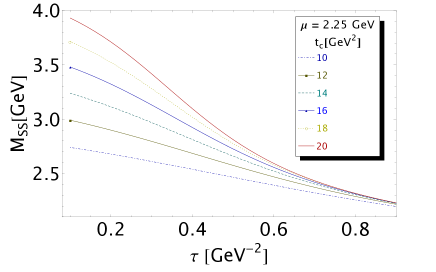
b)

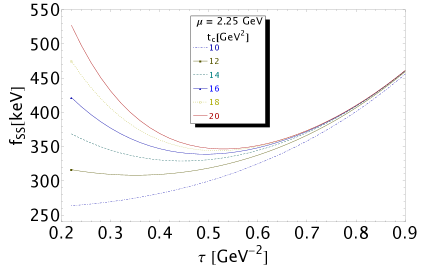
Figure 1: $f_{SS}$ and $M_{SS}$ as function of $\tau$ at NLO for different values of $t_{c}$, $\mu$=2.25 GeV and the values of the QCD parameters given in Ref.[1].

3.2 $\mu$-stability

In Fig. 2, we show the $\mu$-dependence of the results for given $t_{c}$=18 GeV² and $\tau$=0.49 GeV^-2. One finds a common stability for $\mu=(2.25\pm 0.25)$ GeV, which confirms the result in Ref. [4].

a)

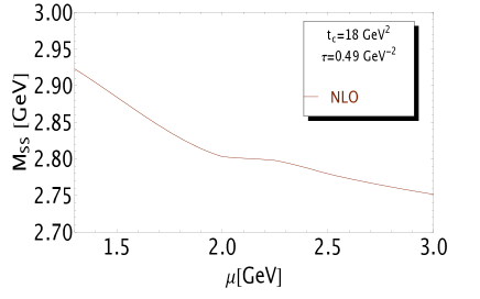
b)

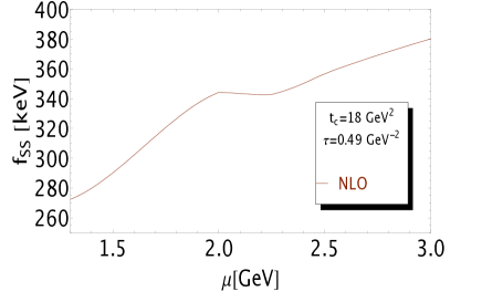
Figure 2: $M_{SS}$ and $f_{SS}$ as function of $\mu$ at NLO for fixed values of $t_{c}$, $\tau$ and the values of the QCD parameters given in Ref. [1].

4 The First Radial Excitation

We extend the analysis in Ref. [4] by using a “Two resonances” + $\theta(t-t_{c})$“QCD continuum” parametrization of the spectral function. To enhance the contribution of the 1st radial excitation, we shall also work with the ratio of moments ${\cal R}_{1}$ in addition to ${\cal R}_{0}$ for getting the masses. We use the same criteria involving the stability points in $(\tau,t_{c},\mu)$ and the optimal results are given in Table 2. We observe that the mass-splittings between the first radial excitation and the lowest ground state are in order of $\sim 1500$ MeV, which is much bigger than $\sim 500$ MeV typically used for ordinary mesons.

5 Understanding LHCb Experimental Data

Our results indicate that the molecules and tetraquark states leading to the same final states are almost degenerated in masses. Therefore, we expect that the “physical state” is a combination of almost degenerated molecules and tetraquark states with the same quantum numbers $J^{PC}$ which we shall call: Tetramole $({\cal T_{M}}_{J})$.

5.1 The $X_{0}(2866)$ and $X_{J}(3150)$ states

Taking literally our results in Table 2, one can see that we have three (almost) degenerate states:

$$\!\!\!\!\!\!\!\!\!\!M_{SS}=2736(21)~{}{\rm MeV},~{}~{}~{}M_{AA}=2675(65)~{}{\rm MeV}~{}~{}$$

$${\rm and}~{}~{}~{}~{}M_{D^{*}K^{*}}=2808(41)~{}{\rm MeV}~{},$$

and their couplings to the corresponding currents are almost the same:

$$\!\!\!\!\!\!\!f_{SS}=345(28)~{}{\rm keV},~{}~{}~{}~{}f_{AA}=498(43)~{}{\rm keV},$$

$${\rm and}~{}~{}~{}~{}~{}f_{D^{*}K^{*}}=405(33)~{}{\rm keV}~{},$$

We assume that the physical state, hereafter called Tetramole $({\cal T_{M}}_{J})$, is a superposition of these nearly degenerated hypothetical states having the same quantum numbers. Taking its mass and coupling as (quadratic) means of the previous numbers, we obtain:

$$M_{{\cal T_{M}}_{0}}\simeq 2743(18)~{}{\rm MeV}~{},~{}~{}~{}f_{{\cal T_{M}}_{0}}\simeq 395(19)~{}{\rm keV}~{}$$

The ${\cal T_{M}}_{0}$ tetramole is a good candidate for explaining the $X_{0}(2866)$ though its mass is slightly lighter.

One can also see from Table 2 that the radial excitation $(DK)_{1}$ mass and coupling are :

$$M_{(DK)_{1}}\simeq 3678(310)~{}{\rm MeV},~{}~{}f_{(DK)_{1}}\simeq 199(62)~{}{\rm keV}$$

which is the lightest $0^{+}$ first radial excitation. Assuming that the $X_{J}(3150)$ bump is a scalar state ($J=0$), we attempt to use a two-component minimal mixing model between the Tetramole $({\cal T_{M}}_{0})$ and the $(DK)_{1}$ radially excited molecule:

$$|X_{0}(2866)\rangle = \cos\theta_{0}|{\cal T_{M}}_{0}\rangle+\sin\theta_{0}|(DK)_{1}\rangle$$

$$|X_{0}(3150)\rangle = -\sin\theta_{0}|{\cal T_{M}}_{0}\rangle+\cos\theta_{0}|(DK)_{1}\rangle~{}.$$

We reproduce the data with a tiny mixing angle :

$$\theta_{0}\simeq(5.2\pm 1.9)^{0}~{}.$$

5.2 The $X_{1}(2904)$ and $X_{J}(3350)$ states

As one can see in Table 2, there are four degenerate states with masses around $\sim 2650$ MeV, and couplings around $\sim 200$ keV. We assume again that the (unmixed) physical state is a combination of these hypothetical states. We evaluate the mass and coupling of this Tetramole as the (geometric) means:

$$M_{{\cal T_{M}}_{1}}=2656(20)~{}{\rm MeV},~{}~{}~{}~{}f_{{\cal T_{M}}_{1}}\simeq 229(12)~{}{\rm keV},$$

where one may notice that it can contribute to the $X_{1}(2904)$ state but its mass is slightly lower. Looking at to the $1^{-}$ radial excitations in Table 2, one can see that they are almost degenerated around 4.5 GeV from which one can extract the masses and couplings (geometric mean) of the spin 1 Tetramoles:

$$\!\!\!\!\!\!\!M_{({\cal T_{M}}_{1})_{1}}\simeq 4592(141)~{}{\rm MeV},~{}~{}~{}f_{({\cal T_{M}}_{1})_{1}}\simeq 223(35)~{}{\rm keV}~{}.$$

Then, we may consider a minimal two-component mixing of the spin 1 Tetramole (${\cal T_{M}}_{1}$) with its 1st radial excitation $({\cal T_{M}}_{1})_{1}$ to explain the $X_{1}(2904)$ state and the $X_{J}(3350)$ bump assuming that the latter is a spin 1 state. The data can be fitted with a tiny mixing angle :

$$\theta_{1}\simeq(9.1\pm 0.6)^{0}~{}.$$

A (non)-confirmation of these two minimal mixing models requires an experimental identification of the quantum numbers of the bumps at 3150 and 3350 MeV.

5.3 Final results

Our final results are obtained at the stability points of the set of parameters $(\tau,t_{c},\mu)$ and they are summarized in Table 2. One can notice that, for some molecule and tetraquark states, the ground state mass values are above $5.5$ GeV which are too far to contribute to the LHCb observations in $DK$ invariant mass. In such cases, the sum rule results are discarded. One can find the full analysis of different sources of errors, as well as an interesting discussion on the relevance of NLO calculations for sum rules in Ref.[1].

Table 2: LSR predictions, at NLO, for the decay constants and masses of the ground state ($f_{0}$, $M_{0}$), and their respective first radial excitation values ($f_{1}$, $M_{1}$), for the molecules and tetraquark states. The symbol “$\ast$” indicates that first radial excitation of high mass ground states were discarded in our sum rule analysis.

Observables	$M_{0}$ (MeV)	$f_{0}$ (keV)	$M_{1}$ (MeV)	$f_{1}$ (keV)
$0^{+}$ States
Molecule
${DK}$	2402(42)	254(48)	3678(310)	211(51)
${D^{*}K^{*}}$	2808(41)	405(33)	4626(252)	568(167)
${D_{1}K_{1}}$	5258(113)	664(57)	$\ast$	$\ast$
${D_{0}^{*}K_{0}^{*}}$	6270(160)	249(18)	$\ast$	$\ast$
Tetraquark
${SS}$	2736(21)	345(28)	4586(268)	359(81)
${AA}$	2675(65)	498(43)	4593(289)	547(95)
${VV}$	5704(149)	713(66)	$\ast$	$\ast$
${PP}$	5917(98)	538(41)	$\ast$	$\ast$
$1^{-}$ States
Molecule
${D_{1}K}$	2676(47)	191(21)	4582(414)	157(71)
${D_{0}^{*}K^{*}}$	2744(41)	216(22)	4662(269)	237(63)
${DK_{1}}$	5377(166)	351(31)	$\ast$	$\ast$
${D^{*}K_{0}^{*}}$	5358(153)	255(23)	$\ast$	$\ast$
Tetraquark
${PA}$	2666(32)	285(29)	4571(213)	258(82)
${SV}$	2593(31)	259(25)	4541(345)	243(68)
${AP}$	5542(139)	416(38)	$\ast$	$\ast$
${VS}$	5698(175)	412(43)	$\ast$	$\ast$

6 Summary and conclusions

$\bullet~{}$ Motivated by the recent LHCb data on the $D^{-}K^{+}$ invariant mass from $B\to D^{+}D^{-}K^{+}$ decay, we have systematically calculated the masses and couplings of some possible configurations of the molecules and tetraquarks states using QCD Laplace sum rules (LSR) within stability criteria where we have added to the LO perturbative term, the NLO radiative corrections, and the contributions from quark and gluon condensates up to dimension-6 in the OPE.

$\bullet~{}$ The peak around the $DK$ threshold can be due to $DK$ scattering amplitude $\oplus$ the $DK(2400)$ lowest mass molecule.

$\bullet~{}$ The ($0^{+}$) $X_{0}(2866)$ and $X_{J}(3150)$ (if it is a $0^{+}$ state) can e.g result from a mixing of the Tetramole (${\cal T_{M}}_{0}$) with the 1st radial excitation $(DK)_{1}$ of the molecule state $(DK)$ with a tiny mixing angle $\theta_{0}\simeq(5.2\pm 1.9)^{0}$.

$\bullet~{}$ The ($1^{-}$) $X_{1}(2904)$ and $X_{J}(3350)$ (if it is a $1^{-}$ state) can result from a mixing of the Tetramole (${\cal T_{M}}_{1}$) with its 1st radial excitation $({\cal T_{M}})_{1}$ with a tiny mixing angle $\theta_{1}\simeq(9.1\pm 0.6)^{0}$.

$\bullet~{}$ More data on the precise quantum numbers of the $X_{J}(3150)$ and $X_{J}(3350)$ states are needed for testing the previous two minimal mixing models proposal.

References

- [1] R.M. Albuquerque, S. Narison, D. Rabetiarivony and G. Randriamanatrika, Nucl. Phys. A 1007 (2021) 122113.
- [2] [LHCb Collab.] R. Aaij et al., Phys.Rev.Lett. 125, 242001 (2020).
- [3] [LHCb Collab.], R. Aaij et al., Phys.Rev. D102, 112003 (2020).
- [4] R. M. Albuquerque et al., Int. J. Mod. Phys. A 31 (2016) 17, 1650093.
- [5] M. Tanabashi et al. (Particle Data Group), Phys. Rev. D 98 (2018) 030001 and 2019 update.
- [6] G.K.C. Cheung et al., arXiv: 2008.06432v1 [hep-lat] (2020).
- [7] H. G. Dosch, M. Jamin and B. Stech, Z. Phys. C42 (1989) 167.
- [8] M. Jamin and M. Neubert, Phys. Lett. B238 (1990) 387.
- [9] J.-R. Zhang, arXiv: 2008.07295 [hep-ph] (2020).
- [10] H.-X. Chen et al., Chin. Phys. Lett. 37 (2020) 101201.
- [11] Z.-W. Wang, Int. J. Mod. Phys. A35 (2020) 2050187.
- [12] W. Chen et al., Phys. Rev. D95 (2017) 114005.
- [13] S.S. Agaev, K. Azizi and H. Sundu, arXiv: 2008.13027 [hep-ph] (2020).
- [14] H. Mutuk, arXiv: 2009.02492 [hep-ph] (2020).
- [15] M.A. Shifman, A.I. Vainshtein and V.I. Zakharov, Nucl. Phys. B147 (1979) 385.
- [16] M.A. Shifman, A.I. Vainshtein and V.I. Zakharov, Nucl. Phys. B147 (1979) 448.
- [17] S. Narison, QCD spectral sum rules, World Sci. Lect. Notes Phys. 26 (1989) 1.
- [18] S. Narison, QCD as a theory of hadrons, Cambridge Monogr. Part. Phys. Nucl. Phys. Cosmol. 17 (2004) 1-778 [hep-ph/0205006].
- [19] S. Narison, Phys. Rept. 84 (1982) 263;
- [20] S. Narison, Acta Phys. Pol. B 26(1995) 687;
- [21] B.L. Ioffe, Prog. Part. Nucl. Phys. 56 (2006) 232.
- [22] L. J. Reinders, H. Rubinstein and S. Yazaki, Phys. Rept. 127 (1985) 1.
- [23] E. de Rafael, les Houches summer school, hep-ph/9802448 (1998).
- [24] F.J Yndurain, The Theory of Quark and Gluon Interactions, 3rd edition, Springer (1999).
- [25] R.A. Bertlmann, Acta Phys. Austriaca 53, (1981) 305.
- [26] P. Pascual and R. Tarrach, QCD: renormalization for practitioner, Springer 1984.
- [27] H.G. Dosch, Non-pertubative Methods, ed. Narison, World Scientific (1985).