Control of superexchange interactions with DC electric fields

Abstract

We discuss DC electric-field controls of superexchange interactions. We first present generic results about antiferromagnetic and ferromagnetic superexchange interactions valid in a broad class of Mott insulators, where we also estimate typical field strength to observe DC electric-field effects: $\sim 1~{}\mathrm{MV/cm}$ for inorganic Mott insulators such as transition-metal oxides and $\sim 0.1~{}\mathrm{MV/cm}$ for organic ones. Next, we apply these results to geometrically frustrated quantum spin systems. Our theory widely applies to (quasi-)two-dimensional and thin-film systems and one-dimensional quantum spin systems on various lattices such as square, honeycomb, triangular, and kagome ones. In this paper, we give our attention to those on the square lattice and on the chain. For the square lattice, we show that DC electric fields can control a ratio of the nearest-neighbor and next-nearest-neighbor exchange interactions. In some realistic cases, DC electric fields make the two next-nearest-neighbor interactions nonequivalent and eventually turns the square-lattice quantum spin system into a deformed triangular-lattice one. For the chain, DC electric fields can induce singlet-dimer and Haldane-dimer orders. We show that the DC electric-field-induced spin gap $\propto|\bm{E}|^{2/3}$ in the Heisenberg antiferromagnetic chain will reach $\sim 10~{}\%$ of the dominant superexchange interaction in the case of a spin-chain compound $\mathrm{KCuMoO_{4}(OH)}$ when the DC electric field of $\sim 1~{}\mathrm{MV/cm}$ is applied.

I Introduction

Controlling quantum states of matter has been a long-standing subject of condensed-matter physics and other related fields. Historically, the condensed-matter-physics community has made much effort for the challenging task of searching for novel quantum states of matter such as, in quantum magnetism, spin liquids Anderson (1973); Savary and Balents (2016); Zhou et al. (2017); Knolle and Moessner (2019); Jiang et al. (2012); Metavitsiadis et al. (2014) and spin-nematic states Chubukov (1991); Shannon et al. (2006); Läuchli et al. (2006); Hikihara et al. (2008); Sudan et al. (2009); Penc and L’́auchli (2011). This task includes a search for experimental realizations of theoretical models that can host such quantum states. However, the synthesis of a compound that faithfully realizes the theoretical model does not mean realizing the quantum phase of our interest, which depends on the parameters of the compound. In general, it is even more challenging to obtain a model compound with a parameter set suitable for realizing the desired phase.

Microscopic controls of quantum states by external forces then become important. External forces can induce a quantum phase transition into the phase of our interest and can bring us the microscopic information of the quantum state through the response to the external forces. An external DC (i.e., static) magnetic field is a typical example. The DC magnetic field adds the Zeeman interaction to the Hamiltonian and induces quantum phase transitions such as Bose-Einstein condensation of magnetic excitations Giamarchi et al. (2008). The pressure is another interesting example. The pressure can change the microscopic parameters of the Hamiltonian without introducing additional interactions Zayed et al. (2017); Sakurai et al. (2018); Zvyagin et al. (2019).

Recently, AC-field controls of quantum states of matter have become a vigorous research subject Oka and Aoki (2009); Kitagawa et al. (2011); Wang et al. (2013); Jotzu et al. (2014). The Floquet theory Shirley (1965); Sambe (1973) provides us with a fundamental framework of such AC-field controls, which are often referred to as the Floquet engineering Bukov et al. (2015); Eckardt (2017); Oka and Kitamura (2019); Sato (2021). The Floquet engineering has also been discussed in quantum magnetism Oka and Kitamura (2019); Takayoshi et al. (2014a, b); Sato et al. (2016); Mentink et al. (2015); Kitamura et al. (2017); Takasan et al. (2017); Claassen et al. (2017); Chaudhary et al. (2019); Sato et al. (2014); Higashikawa et al. (2018).

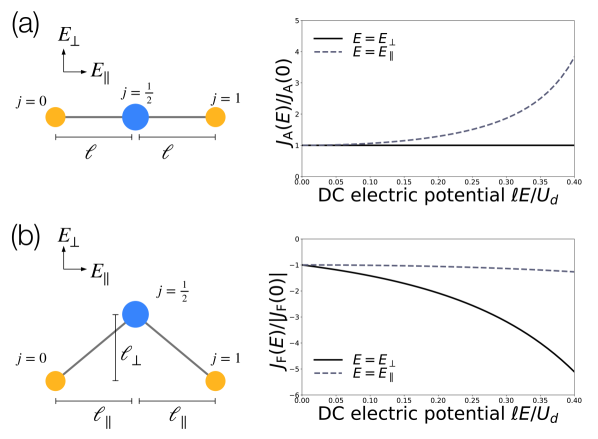
Figure 1: (a) The antiferromagnetic superexchange interaction (17) between two magnetic ions (the orange balls) is plotted as a function of $\ell E/U_{d}$, where $\ell$ is the distance between the $j=0$ ($j=1$) and $j=1/2$ sites, and $U_{d}$ is the on-site Coulomb repulsion at the $d$-orbital sites. We assume that the two magnetic-ion sites and the ligand (the blue ball) site are linearly aligned along the unit vector $\bm{e}_{0,1}$ that connects the $j=0,1$ sites. The DC electric field is applied either parallel ($\bm{E}_{\parallel}$) or perpendicular ($\bm{E}_{\perp}$) to a unit vector $\bm{e}_{0,1}$. (b) When the ligand site is located to form the right angle as shown in the left panel, the superexchange interaction between the magnetic ions can become ferromagnetic. The ferromagnetic interaction (20) is plotted in the right panel. When the DC electric field is applied parallel (perpendicular) to $\bm{e}_{0,1}$, we take $\ell=\ell_{\parallel}$ ($\ell=\ell_{\perp}$, respectively). For (a) and (b), we used typical values, $U_{d}=5$ eV, $U_{p}=1$ eV, and $\Delta_{dp}=2$ eV. Also, we took $J_{\rm H}=U_{p}=1$ eV for (b). The hoppings $t_{0}$ and $t_{1}$ can be arbitrary when we consider ratios $J_{\rm A}(\bm{E})/J_{\rm A}(\bm{0})$ and $J_{\rm F}(\bm{E})/|J_{\rm F}(\bm{0})|$ [see Eqs. (17) and (20)].

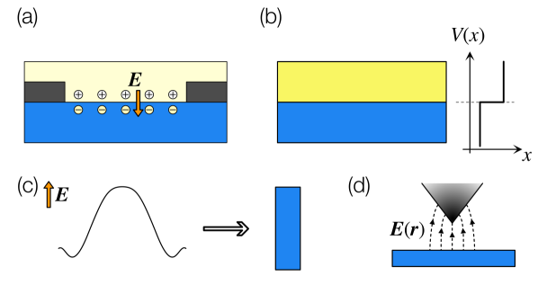
Figure 2: Three exemplary methods to impose a site-dependent potential to a sample. (a) We can employ a field-effect transistor to generate the DC electric field indicated by an orange arrow Ueno et al. (2014); Bisri et al. (2017). (b) A surface potential at a boundary of two different materials can be used as a source of the gradient of the potential $V(x)$ due to the explicit inversion-symmetry breaking at the surface. (c) A single-cycle terahertz laser pulse can also be a DC electric-field source within a time scale sufficiently shorter than the pulse width (see Sec. VI.4.). (d) A needle-like electrode device such as scanning tunneling microscopes can yield a spatially local DC electric field Romming et al. (2013); Hsu et al. (2016). The dashed curves depict electric force lines.

Despite these recent developments, microscopic DC electric-field controls, which should be theoretically simpler than AC ones, are less considered in quantum spin systems partly because these systems are usually realized in Mott insulators where the charge degree of freedom is frozen. The DC electric field actually affects the Hamiltonian of quantum spin systems, as shown in Fig. 1, because the exchange interaction has an electronic origin. The superexchange interaction of spins comes from hoppings of electrons carrying the spin. It also motivates us to study DC electric-field effects that the DC field is free from heating effects that the AC one inevitably induces.

Previously, some of the authors investigated DC electric-field controls of “direct superexchange” interactions , originating from direct hoppings between magnetic ions, by starting from a fundamental electron model, the Hubbard model Takasan and Sato (2019). Reference Takasan and Sato (2019) dealt with the DC electric potential as a site-dependent on-site potential. This treatment of the DC electric field applies to general site-dependent potentials and is convenient to discuss several related phenomena on an equal footing, as shown in Fig. 2. Note that strong DC electric fields are often required to induce sizable effects on magnetism, where the surface geometry [Fig. 2 (b)] Matsukura et al. (2015); Chen et al. (2015) and the single-cycle terahertz (THz) laser pulse [Fig. 2 (c)] Hirori et al. (2011); Mukai et al. (2016); Nicoletti and Cavalleri (2016) are helpful for that purpose. DC electric field generated by these methods can be deemed spatially uniform. Note that we can also apply a local DC electric field to the material, for example, by using a needle-like device [Fig. 2 (d)] Romming et al. (2013); Hsu et al. (2016) 

As of this writing, DC electric-field controls of superexchange interactions mediated by nonmagnetic ions are largely unexplored despite their importance to a broad class of Mott-insulating materials such as transition-metal oxides. Reference Takasan and Sato (2019) discussed DC electric-field controls of exchange interactions, which is focused on controlling the spatial anisotropy by the DC electric field. It was not yet discussed how to control exchange interactions by keeping the spatial anisotropy intact.

This paper develops a theory of DC electric-field controls of superexchange interactions in geometrically frustrated quantum spin systems, starting from simple electron models. We are mainly focused on controlling microscopic Hamiltonian without affecting the dimensionality of the sample, in contrast to our previous work Takasan and Sato (2019). Our theory is widely applicable to (quasi-)two-dimensional thin-film and one-dimensional quantum spin systems on various lattices such as square, honeycomb, triangular, and kagome ones. We discuss basic exemplary applications of our theory to frustrated quantum spin systems on the square lattice and those on the chain.

This paper is organized as follows. In Sec. II, we define two models that give a firm foundation for DC electric-field controls of superexchange interactions in specific cases. In Sec. III, we perform fourth-order perturbation expansions on those two models and derive superexchange interactions in generic forms. Also, we estimate typical values of DC electric-field strength from our results. We apply generic results of Sec. III to specific situations in Secs. IV and V. Section IV is devoted to geometrically frustrated quantum spin systems on the square lattice, where the nearest-neighbor $J_{1}$ and next-nearest-neighbor $J_{2}$ exchange interactions compete with each other (see Sec. IV.1). First, we deal with a simple toy model in Sec. IV.2 to demonstrate controlling a ratio of $J_{1}/J_{2}$ by a DC electric field without affecting the spatial anisotropy. Next, we investigate a more realistic situation corresponding to a compound $\mathrm{BaCdVO(PO_{4})_{2}{}}$ Nath et al. (2008) (Sec. IV.3). To get insight into the essential effects of DC electric fields, we employ an electron model that significantly simplifies the structures of those compounds. The simplified model that emulates the experimental reality is studied in Secs. IV.4 and IV.5. Section V discusses another application of our generic results to frustrated quantum spin chains formed on a CuO₂ chain. We show that the DC electric field induces an alternation of nearest-neighbor exchange interactions, called bond alternation. We discuss experimentally observable consequences of the DC electric-field-induced bond alternation, which turns out to differ from the DC magnetic-field-induced one. Section VI discusses other major DC electric-field effects not incorporated in our analysis. We summarize the paper in Sec. VII.

II Generic models

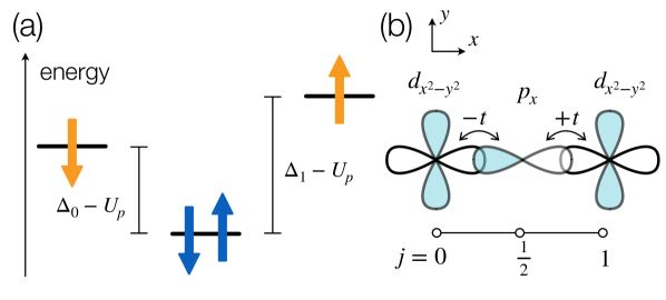
Figure 3: (a) An electron configuration of an unperturbed ground state of the model (2) is schematically drawn. Bars represent the unperturbed energy levels of the $j=0,\frac{1}{2}$, and $1$ site from left to right, whose energy differences are depicted as those among heights. Each bar corresponds to a single orbital. Namely, each bar can have two electrons with the opposite spins. Since the $p$ orbital at the $j=1/2$ site is fully occupied, the eigenenergy is raised by the repulsive potential energy $U_{p}$. (b) Example of the $d$ and $p$ orbitals for the model (2), where the $j=0$ and $1$ sites have the $d_{x^{2}-y^{2}}$ orbital and the $j=1/2$ site has the $p_{x}$ orbital. The hopping amplitudes satisfy $-t_{0}=t_{1}=t$.

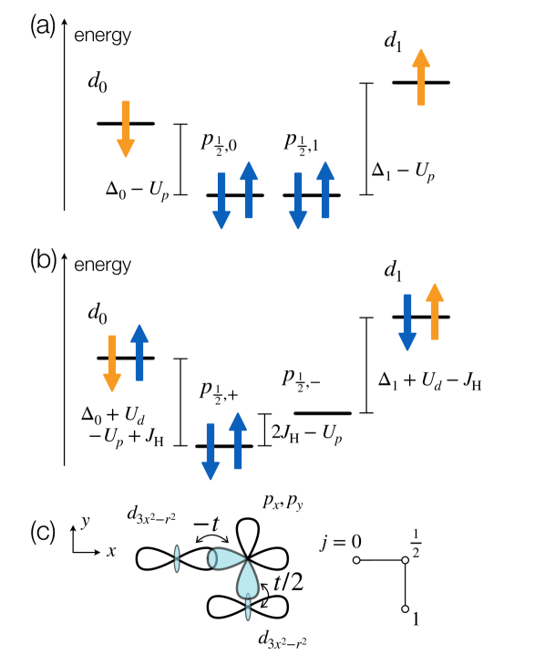
Figure 4: (a) Unperturbed ground state of the model (5). The model has doubly degenerate $p$ orbitals labeled by $p_{\frac{1}{2},0}$ and $p_{\frac{1}{2},1}$ at the $j=1/2$ site unless both of them are half occupied. (b) Unperturbed excited state of the model (5). Since the $p$ orbitals are half occupied, the Coulomb exchange interaction acts on the $p_{\frac{1}{2},\mu}$ orbitals ($\mu=0,1$) and lift their degeneracy by reconstructing them. The reconstructed $p$ orbitals at the $j=1/2$ site are $p_{\frac{1}{2},\pm}=p_{\frac{1}{2},0}\pm p_{\frac{1}{2},1}$. The eigenenergies of the two $p$ orbitals differ by $2J_{\rm H}-U_{p}$ when they are half occupied, that is, when the lower-energy level $p_{\frac{1}{2},+}$ is fully occupied and the higher-energy one $p_{\frac{1}{2},-}$ is empty. (c) Example of the $d$ and $p$ orbitals. Here, we took $d_{0}=d_{1}=d_{3x^{2}-r^{2}}$, $p_{\frac{1}{2},0}=p_{x}$, and $p_{\frac{1}{2},1}=p_{y}$. There are two hoppings, $t_{0}=-t$ between the $d_{3x^{2}-r^{2}}$ and $p_{x}$ orbitals and $t_{1}=\frac{1}{2}t$ between the $d_{3x^{2}-r^{2}}$ and $p_{y}$ orbitals.

Our argument is based on a degenerate perturbation theory of single-band or multi-band Hubbard models with a site-dependent potential, whose Hamiltonian $\mathcal{H}$ is given by the following generic form:

$$\mathcal{H} =\mathcal{H}_{U}+\mathcal{H}_{t}.$$ (1)

Here, $\mathcal{H}_{U}$ represents potential terms such as the on-site Coulomb repulsion and site-dependent potentials, and $\mathcal{H}_{t}$ represents hopping terms of electrons. Note that we include the DC electric field in the site-dependent potential. Throughout the paper, $\mathcal{H}_{t}$ is regarded as a perturbation to $\mathcal{H}_{U}$.

We take two simple and generic models. Both models are made of three sites, two of which have $d$ orbitals, and the other site in the middle has $p$ orbitals. The number of sites is minimized but large enough to yield the superexchange interaction. To discuss the superexchange interaction between $d$ electrons, we assume that each $d$ orbital is half occupied, and the $p$ orbitals are fully occupied in the subspace of the degenerate unperturbed ground states. The difference of two models lies in a degeneracy of $p$ orbitals at the middle site (Figs. 3 and 4).

The first model (Fig. 3) is the three-site single-band Hubbard model with the following Hamiltonian:

$$\mathcal{H}_{\rm A} =\mathcal{H}_{U;\mathrm{A}}+\mathcal{H}_{t;\mathrm{A}},$$ (2)

$$\mathcal{H}_{U;\mathrm{A}} =U_{d}\sum_{j=0,1}n_{j,\uparrow}n_{j,\downarrow}+U_{p}n_{\frac{1}{2},\uparrow}n_{\frac{1}{2},\downarrow}$$

$$\quad+\sum_{j=0,\frac{1}{2},1}\sum_{\sigma}V_{j}n_{j,\sigma}-\frac{h}{2}\sum_{j=0,\frac{1}{2},1}(n_{j,\uparrow}-n_{j,\downarrow}),$$ (3)

$$\mathcal{H}_{t;\mathrm{A}} =-\sum_{\sigma}\{(t_{0}d_{0,\sigma}^{\dagger}+t_{1}d_{1,\sigma}^{\dagger})p_{\frac{1}{2},\sigma}+\mathrm{H.c.}\},$$ (4)

where the $j$th site has a $d$ orbital for $j=0,1$ and a $p$ orbital for $j=1/2$. $d_{j,\sigma}$ and $p_{j,\sigma}$ are annihilation operators of $d$ and $p$ electrons with the spin $\sigma=\uparrow,\downarrow$. Hopping amplitudes, $t_{0},t_{1}\in\mathbb{C}$ are supposed to be complex to incorporate $\mathrm{U(1)}$ fluxes, if necessary. $V_{j}$ represents the site-dependent and spin-independent potential of electrons, into which the DC electric potential enters. Generally, $p$ and $d$ orbitals have different eigenenergies. These atomic orbital eigenenergies are incorporated into our model through the on-site potential term $V_{j}$. The last term of Eq. (3) represents the Zeeman energy, where $h$ is the DC magnetic field. Though $h=g\mu_{B}B$ with $B=\mu_{0}H$ is the Zeeman splitting rather than the DC magnetic field $H$, we roughly identify $h$ and $H$, and call them simply the DC magnetic field in this paper. Both the external magnetic field is spatially uniform. If nonuniform, the exchange interactions would depend on the magnetic field.

We assume that the on-site repulsions $U_{d}>U_{p}>0$ are much larger than $|V_{j}|$ and $|t_{j}|$ to validate a degenerate perturbation expansion about $|t_{j}|/U_{d}$ and $|t_{j}|/U_{p}$. The condition of small $|V_{j}|$ is required to ensure that the low-energy physics involves magnetic excitations only. The same parameter conditions apply to the other model given below.

The second model (Fig. 4) has two $p$ orbtals at the $j=1/2$ site:

$$\mathcal{H}_{\rm F} =\mathcal{H}_{U;\mathrm{F}}+\mathcal{H}_{t;\mathrm{F}},$$ (5)

$$\mathcal{H}_{U;\mathrm{F}} =U_{d}\sum_{j=0,1}n_{j,\uparrow}n_{j,\downarrow}+U_{p}\sum_{\mu=0,1}n_{\frac{1}{2},\uparrow,\mu}n_{\frac{1}{2},\downarrow,\mu}$$

$$\quad+\sum_{j=0,1}\sum_{\sigma}V_{j}n_{j,\sigma}+\sum_{\sigma}\sum_{\mu=0,1}V_{\frac{1}{2}}n_{j,\sigma,\mu}$$

$$\quad-\frac{h}{2}\biggl{[}\sum_{j=0,1}(n_{j,\uparrow}-n_{j,\downarrow})+\sum_{\mu=0,1}(n_{\frac{1}{2},\mu,\uparrow}-n_{\frac{1}{2},\mu,\downarrow})\biggr{]}$$

$$\quad-J_{\rm H}\bm{s}_{0}\cdot\bm{s}_{1},$$ (6)

$$\mathcal{H}_{t;\mathrm{F}} =-\sum_{\sigma}(t_{0}d_{0,\sigma}^{\dagger}p_{\frac{1}{2},\sigma,0}+t_{1}d_{1,\sigma}^{\dagger}p_{\frac{1}{2},\sigma,1}+\mathrm{H.c.}).$$ (7)

The $j=1/2$ site has two $p$ orbitals labeled by the index $\mu=0,1$. The operator $\bm{s}_{\mu}=\frac{\hbar}{2}\sum_{s,s^{\prime}=\uparrow,\downarrow}p_{\frac{1}{2},s,\mu}^{\dagger}\bm{\sigma}^{ss^{\prime}}p_{\frac{1}{2},s^{\prime},\mu}$ denotes the spin-$1/2$ hosted by the $p$ orbital $\mu=0,1$, where $\bm{\sigma}=(\sigma^{x},\,\sigma^{y},\sigma^{z})$ is a set of the Pauli matrices. The operator $\bm{s}_{\mu}$ makes sense only when the $p$ orbitals $\mu=0,1$ are half occupied. We include the interaction, $-J_{\rm H}\bm{s}_{0}\cdot\bm{s}_{1}$, only when both the two $p$ orbitals are half occupied and otherwise may drop it from Eq. (6). The coupling $-J_{\rm H}<0$, which is the ferromagnetic direct exchange between the $p$ orbitals and related to the Hund’s rule, affects the $p$ orbitals only when they are half occupied. Though the inter-band Coulomb potentials are omitted in this model for simplicity, it is straightforward to take them into account.

For simplicity, we focus on a situation where the eigenenergy, $\mathcal{E}_{p}$, of the empty $p$ orbital is equal to or lower than the eigenenergy, $\mathcal{E}_{d}$, of the empty $d$ orbital in both models, that is, $\mathcal{E}_{p}\leq\mathcal{E}_{d}$. These eigenenergies are encoded in the on-site potential $V_{j}$. Here, we introduce a parameter $\Delta_{j}(\bm{E})$ for $j=0,1$,

$$\Delta_{j}(\bm{E}) =V_{j}-V_{\frac{1}{2}}.$$ (8)

$\bm{E}$ denotes the DC electric field, and $\Delta_{j}(\bm{0})=\mathcal{E}_{d}-\mathcal{E}_{p}$ represents the eigenenergy difference of the $d$ orbital at the $j$ site from the $p$ orbital aside from the Coulomb repulsion energy. For example, when we apply $\bm{E}=\bm{E}_{\parallel}$ in Fig. 1 (a), we obtain $\Delta_{0}(\bm{E}_{\parallel})=\mathcal{E}_{d}-\mathcal{E}_{p}-|e|\ell E_{\parallel}$ and $\Delta_{1}(\bm{E}_{\parallel})=\mathcal{E}_{d}-\mathcal{E}_{p}+|e|\ell E_{\parallel}$, where $-e<0$ is the electron charge.

Though we use parameters that meet the condition,

$$\Delta_{j}(\bm{0})\geq 0\quad(j=0,1),$$ (9)

for simplicity throughout this paper, nothing forbids real materials from violating the inequality (9). We emphasize that our results also hold for $\Delta_{j}(\bm{0})<0$. The eigenenergy differences can be shifted by the amount of the Coulomb repulsive energy when the orbitals are partially or fully occupied [Figs. 3 (a) and 4 (a,b)].

We conclude this section by mentioning the orbital degeneracy. We assumed above the single $d$ orbital at each magnetic-ion site, namely, the absence of the $d$-orbital degeneracy. This assumption can be easily relaxed. Let us consider situations where only one $d$ orbital at each magnetic-ion site can participate in hoppings between the intermediate nonmagnetic-ion site because of symmetries. For example, in the setup of Fig. 4 (c), the $p_{x}$ orbital at the $j=0$ has a nonzero hopping amplitude to the $d_{3x^{2}-r^{2}}$ orbital at the $j=1/2$ site and has vanishing hopping amplitude to the other four $d$ orbitals, $d_{xy},\,d_{yz},\,d_{zx},$ and $d_{y^{2}-z^{2}}$. The low-energy physics in these multi-$d$-orbital cases are also effectively described by the models (2) and (5) unless symmetry-breaking structural distortion occurs.

III Superexchange interactions

This section describes the degenerate perturbation theory of the two models (2) and (5) and shows that the former (the latter) model gives rise to a Heisenberg exchange interaction with the antiferromagnetic (ferromagnetic, respectively) coupling.

III.1 Definition of the effective Hamiltonian

The unperturbed ground state is $2^{N}$-fold degenerate for the two models (2) and (5), where $N=2$ is the number of $d$-orbital sites. Let us define a projection operator $P$ onto the subspace of the Hilbert space spanned by the degenerate ground state. $Q=1-P$ is a projection operator onto its complementary space spanned by the unperturbed excited states.

We carry out the perturbation expansion as follows. First, we perform the Schrieffer-Wolf canonical transformation Schrieffer and Wolff (1966) on the full Hamiltonian (1), $\mathcal{H}\to e^{\eta}\mathcal{H}e^{-\eta}$, with an anti-Hermitian operator $\eta$. The effective Hamiltonian $\mathcal{H}_{\rm eff}$ that describes the low-energy physics is then defined as

$$\mathcal{H}_{\rm eff} =Pe^{\eta}\mathcal{H}e^{-\eta}P.$$ (10)

The unitary operator $e^{\eta}$ keeps the excitation spectrum of the model unchanged but can simplify the effective Hamiltonian (10). $\eta$ is determined so that the $e^{\eta}\mathcal{H}e^{-\eta}$ is commutative with $P$ Slagle and Kim (2017). Generic forms of the perturbation expansion of $\mathcal{H}_{\rm eff}$ up to the sixth order are listed in the appendix of Ref. Slagle and Kim (2017).

In our case, a relation, $P\mathcal{H}_{t}P=0$, simplifies the perturbation significantly. Up to the fourth-order perturbation expansion, the effective Hamiltonian (10) is expanded as

$$\mathcal{H}_{\rm eff} =\mathcal{H}_{0}^{\rm eff}+\mathcal{H}_{2}^{\rm eff}+\mathcal{H}_{4}^{\rm eff},$$ (11)

$$\mathcal{H}_{0}^{\rm eff} =P\mathcal{H}_{U}P,$$ (12)

$$\mathcal{H}_{2}^{\rm eff} =P\mathcal{H}_{t}\frac{1}{E_{g}-\mathcal{H}_{U}}Q\mathcal{H}_{t}P,$$ (13)

$$\mathcal{H}_{4}^{\rm eff} =P\mathcal{H}_{t}\biggl{(}\frac{1}{E_{g}-\mathcal{H}_{U}}Q\mathcal{H}_{t}\biggr{)}^{3}P,$$ (14)

where $E_{g}$ is the unperturbed ground-state energy and $(\frac{1}{E_{g}-\mathcal{H}_{U}}Q\mathcal{H}_{t})^{3}$ is an abbreviation of $\frac{1}{E_{g}-\mathcal{H}_{U}}Q\mathcal{H}_{t}\frac{1}{E_{g}-\mathcal{H}_{U}}Q\mathcal{H}_{t}\frac{1}{E_{g}-\mathcal{H}_{U}}Q\mathcal{H}_{t}$. The first- and third-order terms vanish trivially in our models.

The zeroth-order term (12) is mostly constant but contains one important term, the Zeeman energy:

$$\mathcal{H}_{0}^{\rm eff} =-h(S_{0}^{z}+S_{1}^{z})+\mathrm{const}.$$ (15)

$\bm{S}_{j}=\frac{\hbar}{2}\sum_{s,s^{\prime}=\uparrow,\downarrow}d_{j,s}^{\dagger}\bm{\sigma}^{ss^{\prime}}d_{j,s^{\prime}}$ is the $S=1/2$ spin operator at the $j=0,1$ site. Note that the spins of the $p$ orbitals do not appear in Eq. (15) since they are fully occupied in the unperturbed ground-state subspace. The DC magnetic field $h$ appears only in the zeroth-order term (15) because it is spatially uniform and our model Hamiltonians do not have spin-orbit couplings. The second-order term (13) is a constant that has no impact on low-energy physics and thus discarded hereafter.

III.2 Antiferromagnetic superexchange

Performing the fourth-order perturbation expansion on the model (2) (see the Appendix Sec. A.1), we obtain the following effective Hamiltonian:

$$\mathcal{H}_{\rm A}^{\rm eff} =J_{\rm A}(\bm{E})\bm{S}_{0}\cdot\bm{S}_{1}-h(S_{0}^{z}+S_{1}^{z}),$$ (16)

where $J_{\rm A}$ is the antiferromagnetic superexchange interaction,

$$J_{\rm A}(\bm{E}) =2|t_{0}t_{1}|^{2}\biggl{(}\frac{1}{\Delta_{0}(\bm{E})+U_{d}-U_{p}}+\frac{1}{\Delta_{1}(\bm{E})+U_{d}-U_{p}}\biggr{)}^{2}\frac{1}{\Delta_{0}(\bm{E})+\Delta_{1}(\bm{E})+2U_{d}-U_{p}}$$

$$\quad+2|t_{0}t_{1}|^{2}\biggl{(}\frac{1}{(\Delta_{0}(\bm{E})+U_{d}-U_{p})^{2}}\frac{1}{\Delta_{0}(\bm{E})-\Delta_{1}(\bm{E})+U_{d}}+\frac{1}{(\Delta_{1}(\bm{E})+U_{d}-U_{p})^{2}}\frac{1}{\Delta_{1}(\bm{E})-\Delta_{0}(\bm{E})+U_{d}}\biggr{)},$$ (17)

where the DC electric field $\bm{E}$ enters into Eq. (17) through the energy difference $\Delta_{j}(\bm{E})$. When $\bm{E}=\bm{0}$, the Heisenberg superexchange coupling (17) is antiferromagnetic. In fact,

$$J_{\rm A}(\bm{0}) =\frac{4|t_{0}t_{1}|^{2}}{(\Delta_{0}(\bm{0})+U_{d}-U_{p})^{2}}\biggl{(}\frac{2}{2\Delta_{0}(\bm{0})+2U_{d}-U_{p}}+\frac{1}{U_{d}}\biggr{)}$$ (18)

is positive when $\Delta_{j}(\bm{0})\geq 0$ and $U_{d}>U_{p}>0$. The latter inequalities are the case. The former condition (9) is likely to be the case but can be violated, as we mentioned below Eq. (8). Small DC electric field modifies the strength of the antiferromagnetic exchange coupling (17) with keeping its sign.

III.3 Ferromagnetic superexchange

When applied to the model (5), the fourth-order perturbation expansion (appendix A.2) leads to the following effective Hamiltonian of the model (5):

$$\mathcal{H}_{\rm F}^{\rm eff} =J_{\rm F}(\bm{E})\bm{S}_{0}\cdot\bm{S}_{1}-h(S_{0}^{z}+S_{1}^{z}),$$ (19)

where $J_{\rm F}(\bm{E})$ is the DC-electric-field dependent ferromagnetic superexchange interaction,

$$J_{\rm F}(\bm{E}) =-2|t_{0}t_{1}|^{2}\biggl{(}\frac{1}{\Delta_{0}(\bm{E})+U_{d}-U_{p}}+\frac{1}{\Delta_{1}(\bm{E})+U_{d}-U_{p}}\biggr{)}^{2}\frac{J_{\rm H}}{[\Delta_{0}(\bm{E})+\Delta_{1}(\bm{E})+2(U_{d}-U_{p})]^{2}-{J_{\rm H}}^{2}}.$$ (20)

The sign of $J_{\rm F}(\bm{E})$ is determined by that of $J_{\rm H}$. The coupling $J_{\rm H}$ must be positive since it represents the direct Coulomb exchange interaction Koch (2012). The additional condition $\Delta_{0}(\bm{E})+\Delta_{1}(\bm{E})+2(U_{d}-U_{p})-J_{\rm H}>0$ is also required to guarantee that the right hand side of Eq. (20) is negative. The inequality is usually satisfied because $J_{d}/U_{d}=O(1)$, $U_{d}\gg U_{p}$, and $\Delta_{j}(\bm{E})\geq 0$ [Eq. (9)]. When the inequality (9) is violated, the superexchange coupling (20) can become antiferromagnetic. Therefore, the superexchange interaction $J_{\rm F}(\bm{E})$ is ferromagnetic.

III.4 Estimates in typical situations

Here, we estimate the DC electric-field dependence of the antiferromagnetic (17) and ferromagnetic (20) superexchange interaction parameters for typical situations. As Fig. 1 shows, the DC electric field affects the antiferromagnetic (ferromagnetic) superexchange interaction drastically when the DC electric field is applied parallel to $\bm{e}_{\parallel}$ ($\bm{e}_{\perp}$), where the unit vector $\bm{e}_{\parallel}$ ($\bm{e}_{\perp}$) is parallel (perpendicular, respectively) to the vector that connects the $j=0$ site and the $j=1$ site.

Hence, to estimate the typical field strength, we give our attention to the following situations:

$$\bm{E}=E_{\parallel}\bm{e}_{\parallel},$$ (21)

for the antiferromagnetic case (Fig. 3) and

$$\bm{E}=E_{\perp}\bm{e}_{\perp}$$ (22)

for the ferromagnetic case (Fig. 4). Note that the unit vector $\bm{e}_{\perp}$, perpendicular to $\bm{e}_{\parallel}$, is on the plane where $j=0,\frac{1}{2}$, and $1$ sites are put. $J_{\rm A}(\bm{E})$ of Eq. (17) and $J_{\rm F}(\bm{E})$ of Eq. (20) are plotted for $\ell E/U_{d}$ in Fig. 1, where $E$ is either $E_{\perp}$ or $E_{\parallel}$, and $\ell$ is a length scale between the $d$-orbital and the $p$-orbital sites. As shown in Fig. 1 (b), we take $\ell=\ell_{\perp}$ for $E_{\perp}$.

Supposing transition-metal oxides, we employ their typical values $U_{d}=5$ eV, $U_{p}=1$ eV, $\Delta_{dp}=2$ eV, $J_{\rm H}=1$ eV, and $\ell=5$ Å (e.g., Ref. Kim et al. (2017)). Hopping amplitudes $t_{0}$ and $t_{1}$ can be arbitrary, though they should be perturbative.

$J_{\rm A}(\bm{E})$ and $J_{\rm F}(\bm{E})$ depend on the direction of the DC electric field. $J_{\rm A}(\bm{E})$ is sensitive to $E_{\parallel}$ but independent of $E_{\perp}$, which is obvious because the latter case only shifts $V_{j}$ uniformly for $j=0,\frac{1}{2},1$. By contrast, $J_{\rm F}(\bm{E})$ is more sensitive to $E_{\perp}$ than $E_{\parallel}$. To increase $J_{\rm A}(\bm{E})$ and $J_{\rm F}(\bm{E})$ by 1 % of their original values at $\bm{E}=\bm{0}$, we need $\ell|E_{\parallel}|/U_{d}\approx 0.05$ for the former and $\ell_{\perp}|E_{\perp}|/U_{d}\approx 0.003$ for the latter case, namely,

$$|E_{\parallel}| \approx 5~{}\mathrm{MV/cm},$$ (23)

for the antiferromagnetic superexchange and

$$|E_{\perp}| \approx 0.3~{}\mathrm{MV/cm},$$ (24)

for the ferromagnetic superexchange. These values are large but feasible with current experimental techniques. As summarized in Ref. Ueno et al. (2014), the DC electric field in the conventional field-effect transistor setup [Fig. 2 (a)] reaches the order of 1 $\mathrm{MV/cm}$. Also, recently developing techniques, such as the electric double layer transistors, are capable of inducing the electric field stronger than 10 $\mathrm{MV/cm}$ Ueno et al. (2014); Bisri et al. (2017).

Despite these technical developments, realization of the DC electric field with $O(1)~{}\mathrm{MV/cm}$ is still challenging. It is thus important to look into other approaches that facilitate the achievement of the large DC electric field. There are basically two options. One is to use an alternative sample with more suitable parameters. The other is to use an alternative method to induce the DC electric field.

The simplest way in the first option is to reduce the thickness of the sample. If we can use a thin-film sample, we will be able to use larger DC electric field though the electric field is then applied only in a direction perpendicular to the thin film [Fig. 2 (a)]. Reducing the sample thickness meets our purpose of controlling microscopic parameters without changing the composition of the compound. However, for comparison, it is now worth considering the use of a completely different sample to enhance the DC electric-field effects. Recall that the superexchange interactions (17) and (20) are the functions of $\ell E/U_{d}$. Instead of increasing $|E|$, we may increase $\ell/U_{d}$. Organic Mott insulators will be suitable to this purpose for their long $\ell$ and weak $U_{d}$ . Let us assume, for example, $U_{d}=1$ eV, $U_{p}=0.5$ eV, $\Delta_{dp}=0.8$ eV, $\ell=10$ Å (e.g., Refs. Nakamura et al. (2009); Shimizu et al. (2003)). Then, $J_{\rm A}(\bm{E})/J_{\rm A}(\bm{0})$ and $|J_{\rm F}(\bm{E})/J_{\rm F}(\bm{0})|$ are increased by 1 % when

$$E_{\parallel} =0.5~{}\mathrm{MV/cm},$$ (25)

for the antiferromagnetic superexchange and

$$E_{\perp} =0.04~{}\mathrm{MV/cm}$$ (26)

for the ferromagnetic superexchange.

The last option we consider here is to employ an alternative DC electric-field source, the THz laser pulse (Fig. 2), instead of using modifying the sample . The THz laser can induce a larger electric field than the DC one Fülöp et al. (2020). We can regard the THz laser pulse effectively as a DC electric field in a shorter time than the temporal width of the pulse. To adopt the THz laser pulse for the DC electric-field control of quantum magnetic states, we need to use a quantum magnet with fast enough spin dynamics (see Sec. VI.4).

IV Frustrated ferromagnets on square lattice

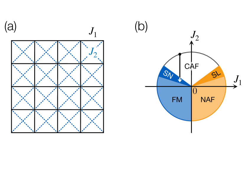
Figure 5: (a) Lattice structure of the spin-$1/2$ $J_{1}$–$J_{2}$ Heisenberg model on the square lattice (27). The spin is put on every crossing of the square and interact with each other via the nearest-neighbor $J_{1}$ interaction (the solid line segment) and the next-nearest-neighbor $J_{2}$ interaction (the dashed line segment). (b) The ground-state phase diagram of the $J_{1}$–$J_{2}$ model (27) Schmidt et al. (2007); Shannon et al. (2006); Jiang et al. (2012). The angle $\theta$ around the origin corresponds to the ratio $J_{1}/J_{2}$: $\tan\theta=J_{2}/J_{1}$. The labels CAF, SN, FM, NAF, and SL are shorthands for the canted antiferromagnetic, spin-nematic, ferromagnetic, Néel antiferromagnetic, and spin-liquid phases, respectively.

Sections IV and V are devoted to applications of the generic results of Sec. III to simple frustrated quantum spin systems.

IV.1 Model

This section deals with a frustrated quantum spin system on the square lattice. We give our attention to a frustrated spin-$1/2$ $J_{1}$–$J_{2}$ model Chandra and Doucot (1988); Dagotto and Moreo (1989); Read and Sachdev (1991); Nomura and Okamoto (1994); Singh et al. (1999); Capriotti and Sorella (2000); Sirker et al. (2006); Ueda and Totsuka (2007); Jiang et al. (2012); Hu et al. (2013); Wang et al. (2016); Wang and Sandvik (2018); Shannon et al. (2006); Shindou et al. (2011); Iqbal et al. (2016); Sato and Morisaku (2020) with the following Hamiltonian,

$$\mathcal{H}_{\rm sq} =J_{1}\sum_{\braket{\bm{r},\bm{r}^{\prime}}_{1}}\bm{S}_{\bm{r}}\cdot\bm{S}_{\bm{r}^{\prime}}+J_{2}\sum_{\braket{\bm{r},\bm{r}^{\prime}}_{2}}\bm{S}_{\bm{r}}\cdot\bm{S}_{\bm{r}^{\prime}},$$ (27)

where $J_{1}$ and $J_{2}$ represent the nearest-neighbor and next-nearest-neighbor interactions, respectively. $\braket{\bm{r},\bm{r}^{\prime}}_{1}$ ($\braket{\bm{r},\bm{r}^{\prime}}_{2}$) denotes a pair of a nearest-neighbor (next-nearest-neighbor, respectively) bond connecting two sites $\bm{r}=(r_{x},\,r_{y})$ and $\bm{r}^{\prime}=(r^{\prime}_{x},\,r^{\prime}_{y})$ of the square lattice [Fig. 5 (a)]. The model (27) is realized in various compounds Melzi et al. (2001); Rosner et al. (2003); Kaul et al. (2004); Bombardi et al. (2004, 2005); Kageyama et al. (2005); Oba et al. (2006); Nath et al. (2008); Tsirlin et al. (2008); Tsirlin and Rosner (2009); Ishikawa et al. (2017)

We can apply the DC magnetic field $h$ to the model (27) through the zeroth-order term (15), but in what follows, we focus on the $h=0$ case. The model (27) shows a rich ground-state phase diagram Schmidt et al. (2007); Shannon et al. (2006) depending on the ratio of $J_{1}$ and $J_{2}$ [Fig. 5 (b)], which contains the spin-liquid phase and the spin-nematic phase. Hereafter, we employ the unit system $\hbar=e=a_{0}=1$ for simplicity, where $-e<0$ is the electron charge and $a_{0}$ is the lattice spacing.

IV.2 Toy model

Before addressing an experimentally feasible case, we first consider a simple toy model on a lattice of Fig. 6 (a) to get insight into the DC electric-field effects on $J_{1}/J_{2}$. The lattice contains edge-sharing pyramids, where the empty balls form a square lattice. Every crossing of the square lattice has one magnetic-ion site with a single $d$ orbital that hosts an $S=1/2$ spin. The top of the pyramid has one ligand site, which is depicted as a filled ball in Fig. 6 (a). We assume that this ligand site hosts two $p$ orbitals. Similarly to the model (5), these $p$ orbitals are fully occupied and degenerate in the unperturbed ground-state subspace. When the system is excited to a state with the half-filled $p$ orbitals, the Coulomb exchange $J_{\rm H}$ lifts the orbital degeneracy. For simplicity, we consider only two hoppings: $t$ on the square edge and $t^{\prime}$ that climbs up the pyramid to the top [Fig. 6 (b)].

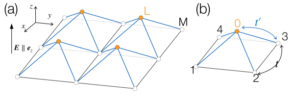
Figure 6: (a) Toy model to demonstrate the DC electric-field control of the ratio $J_{1}/J_{2}$. The $d$ orbitals are put on the square lattice (the white balls) and the $p$ orbitals are put on top of the pyramids (the orange balls). (b) Five-site (single-pyramid) model (28) with two kinds of hoppings, $t$ for the $d$-$d$ hoppings and $t^{\prime}$ for the $d$-$p$ hoppings.

As we did in Sec. III, we minimize the number of sites down to 5 [Fig. 6 (b)] and discuss nearest-neighbor and next-nearest-neighbor exchange interactions of spins. The five-site model on the single pyramid has the following Hamiltonian:

$$\mathcal{H}_{\rm py} =\mathcal{H}_{U;\mathrm{py}}+\mathcal{H}_{t;\mathrm{py}},$$ (28)

$$\mathcal{H}_{U;\mathrm{py}} =U_{d}\sum_{j=1}^{4}n_{j,\uparrow}n_{j,\downarrow}+U_{p}\sum_{\mu=0,1}n_{0,\uparrow,\mu}n_{0,\downarrow,\mu}$$

$$\quad+\sum_{j=0}^{4}\sum_{\sigma}V_{j}n_{j,\sigma},$$ (29)

$$\mathcal{H}_{t;\mathrm{py}} =-\sum_{j=1}^{4}\sum_{\sigma}(td_{j,\sigma}^{\dagger}d_{j+1,\sigma}+\mathrm{H.c.})$$

$$\quad-\sum_{\sigma}[t^{\prime}(d_{1,\sigma}^{\dagger}+d_{3,\sigma}^{\dagger})p_{0,\sigma,1}$$

$$\qquad+t^{\prime}(d_{2,\sigma}^{\dagger}+d_{4,\sigma}^{\dagger})p_{0,\sigma,0}+\mathrm{H.c.}]$$

$$\qquad-J_{\rm H}\bm{s}_{0}\cdot\bm{s}_{1},$$ (30)

where $d_{j,\sigma}^{\dagger}$ for $j=1,2,3$, and $4$ and $p_{0,\sigma,\mu}^{\dagger}$ for $\mu=0,1$ are creation operators of the $d$-orbital electron and the $p$-orbital one, respectively. The index $\mu=0,1$ distinguishes two $p$ orbitals. Note that we employed the periodic boundary condition in Eq. (28), $d_{j+4,\sigma}^{\dagger}=d_{j,\sigma}^{\dagger}$.

Here, we apply the DC electric field to this system so that the electric field points perpendicular to the square lattice. Namely, we assume the following relations among on-site potentials, $V_{j}$:

$$V_{0} =V_{1}-\Delta_{dp}+\ell E,$$ (31)

$$V_{1} =V_{2}=V_{3}=V_{4},$$ (32)

where $\Delta_{dp}=\Delta_{0}(\bm{0})=\mathcal{E}_{d}-\mathcal{E}_{p}\geq 0$ is the eigenenergy difference of the $d$ orbital and the $p$ orbital and $\ell>0$ denotes the height of the $p$-orbital site from the square-lattice plane. The electric field $\bm{E}$ is applied so that

$$\bm{E}=E\bm{e}_{z},$$ (33)

where $\bm{e}_{z}$ is perpendicular to the basal square lattice of the pyramids (Fig. 6). The situation (33) is in contrast to Ref. Takasan and Sato (2019) where the DC electric field is applied within the square-lattice plane.

We designed the Hamiltonian (28) so that the superexchange interaction along the path $1\to 0\to 2$ is ferromagnetic and that along the path $1\to 0\to 3$ is antiferromagnetic. The other superexchange intearctions are determined similarly. Applying the generic results for $\mathcal{H}_{\rm A}$ [Eq. (2)] and $\mathcal{H}_{\rm F}$ [Eq. (5)] to this pyramid, we obtain an effective spin model with the Hamiltonian,

$$\mathcal{H}_{\rm py}^{\rm eff} =\sum_{j=1}^{4}[J_{1}(\bm{E})\bm{S}_{j}\cdot\bm{S}_{j+1}+J_{2}(\bm{E})\bm{S}_{j}\cdot\bm{S}_{j+2}],$$ (34)

with coupling constants,

$$J_{1}(\bm{E}) =\frac{4|t|^{2}}{U_{d}}-8|t^{\prime}|^{4}\biggl{(}\frac{1}{U_{d}-U_{p}+\Delta_{dp}-\ell E}\biggr{)}^{2}$$

$$\qquad\times\frac{J_{\rm H}}{4[U_{d}-U_{p}+\Delta_{dp}-\ell E]^{2}-{J_{\rm H}}^{2}},$$ (35)

$$J_{2}(\bm{E}) =4|t^{\prime}|^{4}\biggl{(}\frac{1}{U_{d}-U_{p}+\Delta_{dp}-\ell E}\biggr{)}^{2}$$

$$\qquad\times\biggl{(}\frac{2}{2U_{d}-U_{p}+2\Delta_{dp}-2\ell E}+\frac{1}{U_{d}}\biggr{)},$$ (36)

within the fourth-order perturbation expansion about the hoppings. Note that we implicitly assumed that the second-order direct superexchange and the fourth-order superexchange interactions are comparable with each other. In other words, we assumed a relation $O(|t|)=O(|t^{\prime}|^{2})$ so that the leading terms of the “direct superexchange” and superexchange interactions are of the same order.

The first term of $J_{1}(\bm{E})$ is the direct superexchange interaction, and the second term is the ferromagnetic superexchange interaction. $J_{2}(\bm{E})$ is the antiferromagnetic superexchange interaction. We can strengthen ($E>0$) or weaken ($E<0$) the exchange interactions thanks to the explicit breaking of the $z\to-z$ inversion symmetry. Since the electric field (33) is antisymmetric in this inversion, the superexchange interactions (35) and (36) can also contain antisymmetric terms under the $z\to-z$ inversion, which is in contrast to the results of Ref. Takasan and Sato (2019). Figure 7 shows how $E$ controls the ratio $J_{1}(\bm{E})/J_{2}(\bm{E})$.

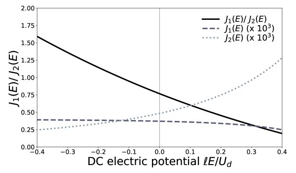
Figure 7: The ratio $J_{1}(\bm{E})/J_{2}(\bm{E})$ is plotted against the DC electric potential $\ell E/U_{d}$. We used parameters: $U_{d}=1$, $U_{p}=J_{\rm H}=0.3$, $\Delta_{dp}=0.5$, $t=0.01$, and $t^{\prime}=0.1$.

IV.3 Motivation from experiments

We demonstrated that the DC electric field indeed controls the ratio of the nearest-neighbor and next-nearest-neighbor interactions of the toy model (28). Since both $J_{1}$ and $J_{2}$ are antiferromagnetic in this model, the DC electric field does not drive the system into the spin-nematic phase [Fig. 5 (b)].

Many experiments were reported about $J_{1}-J_{2}$ square-lattice quantum magnets with $J_{1}<0<J_{2}$, for example, $\mathrm{BaCdVO(PO_{4})_{2}{}}$ Nath et al. (2008); Kohama et al. (2019); Skoulatos et al. (2019) and $A\mathrm{MoOPO_{4}Cl}{}$ ($A=\mathrm{K},\mathrm{Rb}$) Ishikawa et al. (2017). The former compound has $(J_{1},J_{2})\approx(-3.6~{}\mathrm{K},3.2~{}\mathrm{K})$ Nath et al. (2008), which is in the vicinity of the phase boundary between the canted antiferromagnetic phase and the spin-nematic phase. The latter compound has $(J_{1},J_{2})\approx(-2~{}\mathrm{K},19~{}\mathrm{K})$ for $A=\mathrm{K}$ and $(0~{}\mathrm{K},29~{}\mathrm{K})$ for $A=\mathrm{Rb}$ Ishikawa et al. (2017), both of which are supposed to be deep in the canted antiferromagnetic phase.

As we show below, these compounds have characteristic crystal structures that allow for the DC electric-field control of $J_{1}/J_{2}$ in a different mechanism from that for the pyramid model (28). In what follows, we describe the essential characteristics of the crystal structure relevant to our purpose and build a model that simplifies the crystal structure without interfering with the essence.

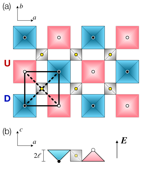
Figure 8: (a) Schematic drawing of the crystal structure of $\mathrm{BaCdVO(PO_{4})_{2}{}}$ projected onto the $ab$ plane Nath et al. (2008). Large blue and red squares represent $\mathrm{VO_{4}}$ pyramids. Small gray squares represent $\mathrm{PO_{4}}$ tetrahedra. Note that oxygen atoms are located on each corner of the squares, which are omitted. We depicted the atoms important for the later discussion of Sec. IV.4. The black and white balls represent the magnetic $\mathrm{V}$ ions and the yellow ones represent the nonmagnetic $\mathrm{P}$ ions. The $V$ ions are located at the top of the pyramid, and the $P$ ions are at the center of the tetrahedron. (b) When the upward and downward pyramids are viewed along the $b$ axis, we find that their magnetic ions are shifted by $2\ell$ ($>0$) along the $c$ axis. This height difference of the magnetic ions plays a crucial role in response to the DC electric field (37).

Figure 8 (a) shows a schematic picture of the crystal structure of $\mathrm{BaCdVO(PO_{4})_{2}{}}$ viewed along the $c$ axis. The single layer that hosts the $J_{1}$–$J_{2}$ model is projected onto the $ab$ plane in this figure. Large squares and small gray squares represent $\mathrm{VO_{4}}$ pyramids and $\mathrm{PO_{4}}$ tetrahedra, respectively [Fig. 8 (b)]. Interestingly, there are two kinds of $\mathrm{VO_{4}}$ pyramids, distinguished by the label U and D in Fig. 8 (a).

The single layer of the $J_{1}$–$J_{2}$ Heisenberg model (27) is composed of U and D pyramids connected by the $\mathrm{PO_{4}}$ tetrahedra Nath et al. (2008). It is crucial in the following argument that the $c$ coordinate of the magnetic ion depends on whether it belongs to the pyramid U or D [Fig. 8 (b)].

To change the ratio $J_{1}/J_{2}$, we apply a uniform DC electric field,

$$\bm{E}=E\bm{e}_{c},$$ (37)

to the system, where $\bm{e}_{c}$ is the unit vector along the $c$ axis. If we define the origin of the electric potential at the height of the $P$ ions, the V ion of the upward pyramid feels the electric potential $-E\ell$ and that of the downward pyramid feels $+E\ell$ with $2\ell>0$ being the height of the pyramid. Though the external field is uniform, the magnetic ion at $\bm{r}=(r_{x},r_{y})$ feels a staggered electric potential $(-1)^{r_{x}+r_{y}}E\ell$ due to the staggered structure of the pyramids [Fig. 8 (a)].

IV.4 Simplified electron model

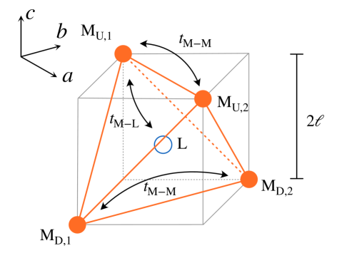
Figure 9: Hopping amplitudes inside a tetrahedron that connects the upper and the lower layers. Magnetic ions (filled balls) on the upward (downward) pyramid are M_I,1 and M_I,2 (M_II,1 and M_II,2). There is a direct hopping $t_{\rm M-M}$ between two magnetic ions that belong to the same kind of pyramid. To hop between two magnetic ions on the two different kinds of pyramids, the electron first hops to the ligand ion (the empty ball) at the center of the tetrahedron and next to the other magnetic ion. The hopping amplitude between the magnetic ion and the ligand is given by $t_{\rm M-L}$.

To investigate DC electric-field effects on $\mathrm{BaCdVO(PO_{4})_{2}{}}$, we develop a model that emulates $\mathrm{BaCdVO(PO_{4})_{2}{}}$ with a much simpler structure. The compound $\mathrm{BaCdVO(PO_{4})_{2}{}}$ has complicated exchange paths between neighboring magnetic V ions. Starting from a V ion site, the path goes through an O ion, a P ion, and another O ion before reaching the other V ion. The miscellaneous O, Ba, and Cd atoms are omitted in Fig. 8. In our simplified model, the miscellaneous atoms of $\mathrm{BaCdVO(PO_{4})_{2}{}}$ are removed. Namely, we consider more direct hoppings between the magnetic ions along paths such as $\mathrm{V\to V}$ or $\mathrm{V\to P\to V}$ as shown in Fig. 9 instead of $\mathrm{V\to O\to P\to O\to V}$. The U and D pyramids are replaced by the magnetic ions with the same labels. Figure 9 represents the U (D) magnetic ions as $\mathrm{M}_{\rm U,1}$ and $\mathrm{M}_{\rm U,2}$ ($\mathrm{M}_{\rm D,1}$ and $\mathrm{M}_{\rm D,2}$, respectively). The ligand site that corresponds to the P ion is also simplified in our model. The ligand site of our model hosts two $p$ orbitals. The Coulomb exchange interaction lifts the orbital degeneracy of the $p$ orbitals when they are half occupied. One of the $p$ orbitals admits hoppings of electrons from/to the $d$ orbitals of the magnetic ions, $M_{\rm U,1}$ and $M_{\rm U,2}$, and the other admits hoppings from/to the $d$ orbitals of the magnetic ions, $M_{\rm D,1}$ and $M_{\rm D,2}$.

Our simplified model inherits the essential structure of $\mathrm{BaCdVO(PO_{4})_{2}{}}$. First, we keep the ligand ion at the center of a tetrahedron formed by the each of four magnetic-ion sites to yield superexchange interactions (Fig. 9). Second, our model has the alternating structure that the magnetic-ion site $\bm{r}=(r_{x},r_{y})$ is located above (below) the ligand site for $r_{x}+r_{y}$ is even (odd) [Fig. 8 (a)].

Figure 10: Lattice deformation by the DC electric field. The $J_{1}$–$J_{2}$ square-lattice model acquires $\delta J_{2}(\bm{E})>0$ from the DC electric field and eventually turns into the deformed triangular-lattice antiferromagnet when $\delta J_{2}$ reaches $J_{2}$.

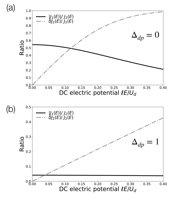
Figure 11: The ratio $J_{1}(\bm{E})/J_{2}(\bm{E})$ of Eqs. (42) and (43) are plotted. In panels (a) and (b), we take $\Delta_{dp}=0$ and $\Delta_{dp}=1$, respectively. The other parameters are taken in common as $U_{d}=1$, $U_{p}=0.5$, $J_{H}=0.5$, $t=0.01$, and $t^{\prime}=0.12$. The ratio $\delta J_{2}(\bm{E})/J_{2}(\bm{E})$ grows with an increase of $\ell E/U_{d}$ for the two cases, where the square lattice becomes the anisotropic triangular lattice. In particular, panel (b) shows that the DC electric field changes only $\delta J_{1}(\bm{E})/J_{2}(\bm{E})$.

Following the generic argument of Sec. III, we minimize the number of sites and consider a five-site electron model with a Hamiltonian,

$$\mathcal{H}_{\rm tetra} =\mathcal{H}_{U;\mathrm{tetra}}+\mathcal{H}_{t;\mathrm{tetra}},$$ (38)

$$\mathcal{H}_{U;\mathrm{tetra}} =U_{d}\sum_{j=1,2}\sum_{\alpha=\mathrm{U,D}}n_{j,\alpha,\uparrow}n_{j,\alpha,\downarrow}$$

$$\qquad+U_{p}\sum_{\alpha=\mathrm{U,D}}n_{\rm L,\alpha,\uparrow}n_{\rm L,\alpha,\downarrow}$$

$$\qquad+\sum_{j=1,2}\sum_{\alpha=\mathrm{U,D}}\sum_{\sigma}V_{\alpha}n_{j,\alpha,\sigma},$$ (39)

$$\mathcal{H}_{t;\mathrm{tetra}} =-\sum_{\sigma}\sum_{\alpha=\mathrm{U,D}}\{(t_{\rm M-M}d_{1,\alpha,\sigma}^{\dagger}d_{2,\alpha,\sigma}+\mathrm{H.c.})$$

$$\quad+[t_{\rm M-L}(d_{1,\alpha,\sigma}^{\dagger}+d_{2,\alpha,\sigma}^{\dagger})p_{\mathrm{L},\alpha,\sigma}+\mathrm{H.c.}]\}$$

$$\qquad-J_{\rm H}\bm{s}_{\rm U}\cdot\bm{s}_{\rm D}.$$ (40)

The model has a $d$ orbital at four magnetic-ion sites at the vertices of the tetrahedron and two orbitals at the ligand site at the center. $d_{j,\alpha,\sigma}^{\dagger}$ represents the annihilation operator of electron at the magnetic-ion site $j$ with the spin $\sigma$. The index $\alpha=\mathrm{U,D}$ indicates the upward and downward magnetic ions, respectively. Accordingly, the on-site potential is given by $V_{\rm U}=\bar{V}-\ell E$ and $V_{\rm D}=\bar{V}+\ell E$ with an $\bm{E}$-independent constant $\bar{V}$. The $p_{\mathrm{L},\alpha,\sigma}$ operator annihilates the $p$ electron at the ligand site. As the hopping term (40) shows, the $p$ orbitals labeled by the index $\alpha=\mathrm{U,D}$ have a hopping term from/to the $d$ orbital with the same $\alpha$ index. $-J_{\rm H}<0$ is the Coulomb exchange interaction between $\bm{s}_{\alpha}=\frac{1}{2}\sum_{s,s^{\prime}}p_{\mathrm{L},\alpha,s}^{\dagger}\bm{\sigma}^{s,s^{\prime}}p_{\mathrm{L},\alpha,s^{\prime}}$ for $\alpha=\mathrm{U,D}$ at the ligand site.

IV.5 Effective spin model

The low-energy effective Hamiltonian of the model (38) is given by

$$\mathcal{H}_{\rm tetra}^{\rm eff} =J_{1}(\bm{E})(\bm{S}_{\rm U,1}+\bm{S}_{\rm U,2})\cdot(\bm{S}_{\rm D,1}+\bm{S}_{\rm D,2})$$

$$\quad+J_{2}(\bm{E})(\bm{S}_{\rm U,1}\cdot\bm{S}_{\rm U,2}+\bm{S}_{\rm D,1}\cdot\bm{S}_{\rm D,2})$$

$$\quad+\delta J_{2}(\bm{E})(\bm{S}_{\rm U,1}\cdot\bm{S}_{\rm U,2}-\bm{S}_{\rm D,1}\cdot\bm{S}_{\rm D,2}).$$ (41)

We dealt with the hoppings by $t_{\rm M-M}$ and $t_{\rm M-L}$ as perturbations to the remainder of the Hamiltonian.

Let us embed the effective model (41) on the tetrahedron into the square lattice of Fig. 5 (a). $J_{1}(\bm{E})$ and $J_{2}(\bm{E})$ are the nearest-neighbor and the next-nearest-neighbor interactions, respectively. The perturbation expansion gives a side effect that the effective Hamiltonian (41) contains the third interaction of $\delta J_{2}(\bm{E})$, which makes the two diagonal bonds nonequivalent (the middle panel of Fig. 10). The appearance of nonzero $\delta J_{2}(\bm{E})$ is due to the explicit violation of an inversion symmetry by $\bm{E}$. When $\bm{E}=\bm{0}$, the bond connecting $\mathrm{M_{U,1}}$ and $\mathrm{M_{U,2}}$ is symmetrically equivalent to that connecting $\mathrm{M_{D,1}}$ and $\mathrm{M_{D,2}}$. The DC electric field along the $c$ axis makes these bonds nonequivalent, that is, $\delta J_{2}(\bm{E})\not=0$. Figure 11 shows the DC electric-field dependence of the exchange interaction for some parameter sets.

The nearest-neighbor interaction is a superexchange interaction, and the next-nearest-neighbor interaction is mainly a direct superexchange interaction though its subleading terms are superexchange ones as shown below. Up to the fourth order of the perturbation expansion, $J_{1}(\bm{E})$, $J_{2}(\bm{E})$, and $\delta J_{2}(\bm{E})$ are given by

$$J_{1}(\bm{E}) =-2|t_{\rm M-L}|^{4}\biggl{(}\frac{1}{U_{d}-U_{p}+\Delta_{dp}-\ell E}+\frac{1}{U_{d}-U_{p}+\Delta_{dp}+\ell E}\biggr{)}^{2}\frac{J_{\rm H}}{[2(U_{d}-U_{p}+\Delta_{dp})]^{2}-{J_{\rm H}}^{2}},$$ (42)

$$J_{2}(\bm{E}) =\frac{4|t_{\rm M-M}|^{2}}{U_{d}}+|t_{\rm M-L}|^{4}\biggl{[}\biggl{(}\frac{2}{U_{d}-U_{p}+\Delta_{dp}-\ell E}\biggr{)}^{2}\frac{1}{2U_{d}-U_{p}+2\Delta_{dp}-2\ell E}$$

$$\qquad+\biggl{(}\frac{2}{U_{d}-U_{p}+\Delta_{dp}+\ell E}\biggr{)}^{2}\frac{1}{2U_{d}-U_{p}+2\Delta_{dp}+2\ell E}$$

$$\qquad+\frac{2}{U_{d}}\biggl{\{}\biggl{(}\frac{1}{U_{d}-U_{p}+\Delta_{dp}-\ell E}\biggr{)}^{2}+\biggl{(}\frac{1}{U_{d}-U_{p}+\Delta_{dp}+\ell E}\biggr{)}^{2}\biggr{\}}\biggr{]},$$ (43)

$$\delta J_{2}(\bm{E}) =|t_{\rm M-L}|^{4}\biggl{[}\biggl{(}\frac{2}{U_{d}-U_{p}+\Delta_{dp}-\ell E}\biggr{)}^{2}\frac{1}{2U_{d}-U_{p}+2\Delta_{dp}-2\ell E}-\biggl{(}\frac{2}{U_{d}-U_{p}+\Delta_{dp}+\ell E}\biggr{)}^{2}\frac{1}{2U_{d}-U_{p}+\Delta_{dp}+2\ell E}$$

$$\qquad+\frac{2}{U_{d}}\biggl{\{}\biggl{(}\frac{1}{U_{d}-U_{p}+\Delta_{dp}-\ell E}\biggr{)}^{2}-\biggl{(}\frac{1}{U_{d}-U_{p}+\Delta_{dp}+\ell E}\biggr{)}^{2}\biggr{\}}\biggr{]}.$$ (44)

$J_{1}(\bm{E})$ and $J_{2}(\bm{E})$ are even functions of $E$ as they should be from the symmetry point of view. By contrast, $\delta J_{2}(\bm{E})$ is an odd function of $E$. Just like we did in Eqs. (35) and (36), we assumed that $O(|t_{\rm M-M}|)=O(|t_{\rm M-L}|^{2})$ to make the leading terms of the exchange and superexchange interactions comparable.

The side effect of nonzero $\delta J_{2}(\bm{E})$ is an interesting phenomenon by itself. In the extreme situation of $\delta J_{2}=J_{2}$, the spin model turns into a deformed triangular-lattice Heisenberg antiferromagnet (Fig. 10) Coldea et al. (2001); Starykh and Balents (2007); Bishop et al. (2009). Each triangle unit has one $J_{2}$ bond and two $J_{1}$ bonds. We can thus expect that the DC electric field changes the square-lattice antiferromagnet eventually into the triangular-lattice one. The deformed triangular-lattice antiferromagnet also exhibits a rich phase diagram under magnetic fields Starykh and Balents (2007). It will be interesting to apply the DC electric and magnetic fields simultaneously to the model (38), searching for $\bm{E}$-induced quantum phase transitions.

We emphasize that the argument in Secs. IV.4 and IV.5 also applies to $A\mathrm{MoOPO_{4}Cl}{}$. There are minor differences between $\mathrm{BaCdVO(PO_{4})_{2}{}}$ and $A\mathrm{MoOPO_{4}Cl}{}$ from the DC electric-field viewpoint. $A\mathrm{MoOPO_{4}Cl}{}$ has the Mo ion whose $4f$ orbital contributes to quantum magnetism, however, which can be dealt with on equal footing with the model (38). The orbital hosting the $S=1/2$ spin does not need to have the $d$-orbital symmetry though we used the notation of the $d$ orbital symbolically. Our model here as well as the generic ones of Sec. II assume that the orbital at the magnetic-ion site is nondegenerate and has a large on-site repulsion, $U_{d}>U_{p}$. The $4f$ orbital fulfills this assumption.

$\mathrm{BaCdVO(PO_{4})_{2}{}}$ and $A\mathrm{MoOPO_{4}Cl}{}$ have the same characteristics in response to the DC electric field for the following reasons. First, $A\mathrm{MoOPO_{4}Cl}{}$ also has two kinds of magnetic-ion sites with two different electric potential energies. Instead of the upward and downward pyramids, $A\mathrm{MoOPO_{4}Cl}{}$ has two kinds of octahedra shifted in the opposite direction along the $c$ axis that results in the same staggered electric-field potential $(-1)^{r_{x}+r_{y}}\ell E$ as $\mathrm{BaCdVO(PO_{4})_{2}{}}$. Second, the same simplification of the hopping paths to Fig. 9 applies to $A\mathrm{MoOPO_{4}Cl}{}$ as well as $\mathrm{BaCdVO(PO_{4})_{2}{}}$. We can expect that the simplification works even better in $A\mathrm{MoOPO_{4}Cl}{}$ thanks to the outspread probability distribution of the $4f$ orbital. We thus conclude that the results (42), (43), and (44) will thus hold also for $A\mathrm{MoOPO_{4}Cl}{}$.

V Frustrated ferromagnetic chains

V.1 Experimental realizations

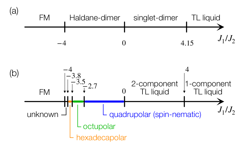
Figure 12: Schematic phase diagrams of the $J_{1}-J_{2}$ spin-$1/2$ chain (45) with $J_{2}>0$ (a) at zero magnetic field Furukawa et al. (2010a) and (b) near the saturation field Kecke et al. (2007); Hikihara et al. (2008); Sudan et al. (2009). (a) The zero-field ground-state phase diagram contains the Tomonaga-Luttinger (TL) liquid, the singlet-dimer, the Haldane-dimer, and the ferromagnetically ordered (FM) phases Nomura and Okamoto (1994); Furukawa et al. (2012). Around the origin, $J_{1}/J_{2}=0$, the gapped phases with two different spontaneous dimer orders appear. The dimers are formed on nearest-neighbor ($J_{1}$) bonds in both phases. (b) When the magnetic field $h$ is in the vicinity of the saturation field, the phase diagram becomes rich. The phase diagram contains quasi-long-range multipolar order phases of spins, the quadrupolar, octapolar, and hexadecapolar phases for $J_{1}<0$ Kecke et al. (2007); Hikihara et al. (2008). In particular, the quadrupolar phase is known as the (quasi-long-range) spin-nematic phase Hikihara et al. (2008); Sudan et al. (2009); Zhitomirsky and Tsunetsugu (2010); Sato et al. (2009, 2011a, 2011b, 2013); Hirobe et al. (2019); Sato and Morisaku (2020); Furuya (2017). There are one- and two-component TL-liquid phases for $J_{1}/J_{2}>4$ and $0<J_{1}/J_{2}<4$, respectively Okunishi (2008); Hikihara et al. (2010).

This section discusses another important frustrated quantum spin system of an $S=1/2$ $J_{1}$–$J_{2}$ spin chain described by the Hamiltonian

$$\mathcal{H}_{\rm chain} =J_{1}\sum_{j}\bm{S}_{j}\cdot\bm{S}_{j+1}+J_{2}\sum_{j}\bm{S}_{j}\cdot\bm{S}_{j+2}-h\sum_{j}S_{j}^{z}.$$ (45)

$J_{1}<0<J_{2}$ cases Hikihara et al. (2008); Sudan et al. (2009); Furukawa et al. (2010b, a); Sato et al. (2011b); Parvej and Kumar (2017) and $J_{1},J_{2}>0$ cases Nomura and Okamoto (1994); Okunishi (2008); Hikihara et al. (2010) have been intensively studied. Figure 12 (a) shows the ground-state phase diagram of the model (45) at $h=0$. It contains two kinds of dimer phases. The sign of $J_{1}$ governs the nature of these dimers. The dimer is a nonmagnetic singlet type for $J_{1}>0$ and a magnetic triplet type for $J_{1}<0$ Furukawa et al. (2012).

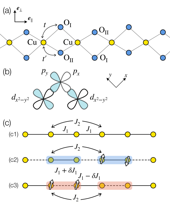
Figure 13: (a) CuO₂ chain with two nonequivalent oxygens, O_I and $O_{\rm II}$. The angles $\angle\mathrm{Cu-O_{I}-Cu}$ and $\angle\mathrm{Cu-O_{II}-Cu}$ are supposed to be site-independent and differ from each other. Accordingly, the CuO₂ chain has the twofold screw symmetry in the $\bm{e}_{\parallel}$ direction along which the chain extends. (b) $3d_{x^{2}-y^{2}}$ orbital of Cu ions and $2p_{x,y}$ orbitals of O ions. When the angle formed by two coppers and one oxygen equals exactly $90^{\circ}$ as shown here, the electron can hop from the left (right) Cu ion to the $p_{x}$ ($p_{y}$, respectively) orbital of the O ion. (c) The $J_{1}$–$J_{2}$ spin chain and the $\bm{E}$-induced dimer states are schematically shown. (c1) The $J_{1}$–$J_{2}$ chain in the absence of the DC electric field (46). (c2) When $J_{1}>0$, the DC electric field (46) with $E>0$ yields the bond alternation $\delta J_{1}>0$, which results in the singlet-dimer ground state. The singlet dimer is formed on the $J_{1}+\delta J_{1}$ bond. (c3) When $J_{1}<0$, the DC electric field (46) with $E>0$ yields the bond alternation $\delta J_{1}>0$, which results in the Haldane-dimer ground state. The Haldane dimer is formed on the $J_{1}-\delta J_{1}$ bond.

Some materials with CuO₂ chains Enderle et al. (2005); Naito et al. (2007); Yasui et al. (2011); Schäpers et al. (2013); Hase et al. (2004); Matsui et al. (2017); Nawa et al. (2015) are known to be described by the $J_{1}-J_{2}$ chain with $J_{1}<0$. When $-2.7<J_{1}/J_{2}<0$, this spin chain has the spin nematic phase in the vicinity of the fully polarized phase forced by the strong magnetic field $h$ [Fig. 12 (b)].

V.2 Goodenough-Kanamori rule

The model (45) can experimentally be realized, for example, in a CuO₂ chain of Fig. 13 (a), where the Cu ion carries the $S=1/2$ spin. Figure 13 (a) shows a generic case that two O ions, O_I and O_II, are nonequivalent. Two O ions can be equivalent but, in what follows, are supposed to be nonequivalent to derive the antiferromagnetic $J_{1}$ and ferromagnetic $J_{1}$ from the single model.

The sign $J_{1}$ is determined by the angle $\angle\mathrm{Cu-O-Cu}$. The two O ions mediate the nearest-neighbor superexchange interaction. According to the Goodenough-Kanamori rule Goodenough (1955); Kanamori (1957a, b), the superexchange interaction is ferromagnetic when an angle $\angle\mathrm{Cu-O-Cu}$ is $90^{\circ}$ and antiferromagnetic when the angle is $180^{\circ}$. We can easily understand this difference by looking into the $d$ and $p$ orbitals of Fig. 13 (b). When the angle is $90^{\circ}$, there are no hoppings between the $d_{x^{2}-y^{2}}$ orbital of the Cu ion and the $p_{x}$ orbital of the O ion. Then, the superexchange interaction is well described by the model (5) with the two degenerate $p$ orbitals at the oxygen site. On the other hand, when the angle is $180^{\circ}$, the single $p$ orbital allows for hoppings of electrons from the O ion to the two Cu ions on both sides. Then, the superexchange interaction is modeled by Eq. (2) with the nondegenerate $p$ orbital at the oxygen site [see also Fig. 3 (b) and Fig. 4 (c)].

Generally, the angles are intermediate, when the superexchange process also has an intermediate character of the two models (2) and (5). For simplicity, we consider an ideal situation where the superexchange interaction via the O_I ion is described by the model (5) with $t_{0}=t_{1}=t$ and that via the O_II ion is described by the model (2) with $t_{0}=t_{1}=t^{\prime}$ [Fig. 13 (a)]. It follows from the above modeling that $0<\angle\mathrm{Cu-O_{I}-Cu}<\angle\mathrm{Cu-O_{II}-Cu}\leq 180^{\circ}$. We assume that the two oxygens are exactly in the middle of the two nearest-neighbor Cu ions along the chain direction, $\bm{e}_{\parallel}$.

V.3 Twofold screw symmetry

When the CuO₂ plane has two nonequivalent oxygen sites, the CuO₂ chain has a twofold screw symmetry along the chain direction, a combination of the discrete translation symmetry in the chain direction and the $\pi$ spatial rotation around that direction. Let us denote the discrete translation as $T_{1}$ and the $\pi$ rotation as $R_{\pi}$. The CuO₂ chain of Fig. 13 (a) has neither $T_{1}$ nor $R_{\pi}$ symmetries though it has the $T_{1}R_{\pi}$ symmetry. Nevertheless, the low-energy spin-chain model (45) in the absence of the electric field has both the $T_{1}$ and $R_{\pi}$ symmetries instead when the electric potentials at the two oxygen sites are exactly balanced.

The DC electric field can violate this balance, replacing the emergent high symmetry of the spin chain by the original $T_{1}R_{\pi}$ one of the CuO₂ chain. Let us apply the following DC electric field to the system,

$$\bm{E}=E\bm{e}_{\perp},$$ (46)

along the direction perpendicular to the CuO₂ chain and on the CuO₂ plane [Fig. 13 (a)]. We denote the electric potentials at the Cu, O_I, and O_II sites as $0$, $\pm\ell_{\rm I}E$, and $\mp\ell_{\rm II}E$, respectively. The sign of the latter two potentials is positive if the O ion is below the Cu ion in the $\bm{e}_{\perp}$ direction and negative if the O ion is above the Cu ion. We can assume $\ell_{\rm I}>\ell_{\rm II}$ to be consistent with the assumption of $\angle\mathrm{Cu-O_{I}-Cu}<\angle\mathrm{Cu-O_{II}-Cu}$.

The effective spin-chain model under the DC electric field (46) has the following Hamiltonian,

$$\mathcal{H}_{\rm chain} =J_{1}(\bm{E})\sum_{j}\bm{S}_{j}\cdot\bm{S}_{j+1}+J_{2}(\bm{E})\sum_{j}\bm{S}_{j}\cdot\bm{S}_{j+1}$$

$$\qquad-h\sum_{j}S_{j}^{z}+\delta J_{1}(\bm{E})\sum_{j}(-1)^{j}\bm{S}_{j}\cdot\bm{S}_{j+1},$$ (47)

where the last term, called the bond alternation, is a direct consequence of the imbalance of the electric potentials of O_I and O_II. The nearest-neighbor interactions, $J_{1}(\bm{E})$ and $\delta J_{1}(\bm{E})$, are given by

$$J_{1}(\bm{E}) =-4|t|^{4}\biggl{[}\biggl{(}\frac{1}{U_{d}-U_{p}+\Delta_{dp}-\ell_{\rm I}E}\biggr{)}^{2}\frac{J_{\rm H}}{4(U_{d}-U_{p}+\Delta_{dp}-\ell_{\rm I}E)^{2}-{J_{\rm H}}^{2}}$$

$$\qquad+\biggl{(}\frac{1}{U_{d}-U_{p}+\Delta_{dp}+\ell_{\rm I}E}\biggr{)}^{2}\frac{J_{\rm H}}{4(U_{d}-U_{p}+\Delta_{dp}+\ell_{\rm I}E)^{2}-{J_{\rm H}}^{2}}\biggr{]}$$

$$\quad+2|t^{\prime}|^{4}\biggl{[}\biggl{(}\frac{1}{U_{d}-U_{p}++\Delta_{dp}+\ell_{\rm II}E}\biggr{)}^{2}\biggl{(}\frac{2}{2U_{d}-U_{p}+2\Delta_{dp}+2\ell_{\rm II}E}+\frac{1}{U_{d}}\biggr{)}$$

$$\qquad+\biggl{(}\frac{1}{U_{d}-U_{p}+\Delta_{dp}-\ell_{\rm II}E}\biggr{)}^{2}\biggl{(}\frac{2}{2U_{d}-U_{p}+2\Delta_{dp}-2\ell_{\rm II}E}+\frac{1}{U_{d}}\biggr{)}\biggr{]},$$ (48)

$$\delta J_{1}(\bm{E}) =-4|t|^{4}\biggl{[}\biggl{(}\frac{1}{U_{d}-U_{p}+\Delta_{dp}-\ell_{\rm I}E}\biggr{)}^{2}\frac{J_{\rm H}}{4(U_{d}-U_{p}+\Delta_{dp}-\ell_{\rm I}E)^{2}-{J_{\rm H}}^{2}}$$

$$\qquad-\biggl{(}\frac{1}{U_{d}-U_{p}+\Delta_{dp}+\ell_{\rm I}E}\biggr{)}^{2}\frac{J_{\rm H}}{4(U_{d}-U_{p}+\Delta_{dp}+\ell_{\rm I}E)^{2}-{J_{\rm H}}^{2}}\biggr{]}$$

$$\quad+2|t^{\prime}|^{4}\biggl{[}\biggl{(}\frac{1}{U_{d}-U_{p}+\Delta_{dp}+\ell_{\rm II}E}\biggr{)}^{2}\biggl{(}\frac{2}{2U_{d}-U_{p}+2\Delta_{dp}+2\ell_{\rm II}E}+\frac{1}{U_{d}}\biggr{)}$$

$$\qquad-\biggl{(}\frac{1}{U_{d}-U_{p}+\Delta_{dp}-\ell_{\rm II}E}\biggr{)}^{2}\biggl{(}\frac{2}{2U_{d}-U_{p}+2\Delta_{dp}-2\ell_{\rm II}E}+\frac{1}{U_{d}}\biggr{)}\biggr{]}.$$ (49)

We emphasize that Eqs. (48) and (49) rely on the assumption that the superexchange mediated by the O_I ion is the ferromagnetic one [Eq. (20)] and the one by the O_II ion is the antiferromagnetic one [Eq. (17)]. $J_{1}(\bm{E})$ and $\delta J_{1}(\bm{E})$ are even and odd functions of $E$, respectively (Figs. 14 and 15). This $E$ dependence is consistent with the twofold screw symmetry of the CuO₂ chain. For instance, since $R_{\pi}$ maps $\bm{E}=E\bm{e}_{\perp}$ to $-\bm{E}$, the $T_{1}R_{\pi}$ operator maps the bond alternation $\delta J_{1}(\bm{E})\sum_{j}(-1)^{j}\bm{S}_{j}\cdot\bm{S}_{j+1}$ to $\delta J_{1}(-\bm{E})\sum_{j}(-1)^{j}\bm{S}_{j+1}\cdot\bm{S}_{j+2}=\delta J_{1}(\bm{E})\sum_{j}(-1)^{j+1}\bm{S}_{j+1}\cdot\bm{S}_{j+2}$. Hence, the $\bm{E}$-induced bond alternation has the twofold screw symmetry though it breaks the $T_{1}$ symmetry.

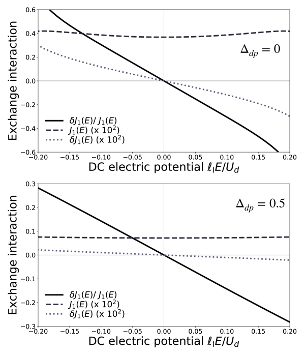
Figure 14: The $\bm{E}$-induced bond alternation $\delta J_{1}(\bm{E})$ is plotted for the DC electric potential $\ell_{\rm I}E$ for the $J_{1},J_{2}>0$ case with parameters, $U_{d}=1$, $U_{p}=0.5$, $J_{H}=0.5$, $t=0.04$, $t^{\prime}=0.1$, and $\ell_{\rm II}/\ell_{\rm I}=0.60$. The ratio $\ell_{\rm II}/\ell_{\rm I}$ is determined from the data for $\mathrm{KCuMoO_{4}(OH)}$ Nawa et al. (2015). We took $\Delta_{dp}=0$ for the upper panel and $\Delta_{dp}=0.5$ for the lower panel.

Note that the right-hand side of Eq. (49) does not vanish for $\ell_{\rm I}=\ell_{\rm II}$, though it should from the symmetry viewpoint. This inconsistency comes from the initial assumption that we made. We assumed that the superexchange process via the O_I ion and that via the O_II ion are supposed to be nonequivalent from the beginning. Accordingly, Eqs. (48) and (49) hold when the difference $\ell_{\rm I}-\ell_{\rm II}$ is large enough to justify the nonequivalent superexchange processes. This condition $\ell_{\rm I,II}$ is convenient for our purpose of the DC electric-field control.

$J_{2}(\bm{E})$ depends on $\bm{E}$ in a complex manner. However, its DC electric-field dependence is less important than the induction of the bond alternation because the latter is much more relevant in the renormalization-group sense Giamarchi (2004); Gogolin et al. (2004).

Before describing the $\bm{E}$-induced bond alternation effects, we comment on the field direction. If we apply the DC electric field along the chain direction ($\bm{e}_{\parallel}$ of Fig. 13), the DC electric field does not yield the bond alternation because it keeps the balance of the electric potentials at the two oxygen sites. The DC electric field $\bm{E}\parallel\bm{e}_{\parallel}$ purely changes the ratio $J_{1}(\bm{E})/J_{2}(\bm{E})$, keeping $\delta J_{1}(\bm{E})=0$, which will be relevant to studies of the quasi-long-range spin-nematic phase of $J_{1}-J_{2}$ spin chains.

V.4 Dimerization induced by DC electric fields

V.4.1 $J_{1}>0$: singlet dimers

When both $J_{1}$ and $J_{2}$ are positive, the ground-state phase diagram for $E=h=0$ contains two phases: a Tomonaga-Luttinger (TL) liquid phase Giamarchi (2004); Gogolin et al. (2004) and a spontaneously dimerized phase. A quantum critical point, $J_{2}/J_{1}=\alpha_{c}\approx 0.2411$ Okamoto and Nomura (1992); White and Affleck (1996), separates these two phases: the TL-liquid phase for $J_{2}/J_{1}\leq\alpha_{c}$ and the spontaneously dimerized phase for $\alpha_{c}<J_{2}/J_{1}$. The former is gapless, and the latter is gapped. Turning on the DC electric field (46), we can introduce the bond alternation to the $J_{1}$–$J_{2}$ spin chain. Trivially, the bond alternation turns the spontaneously dimerized phase into an induced dimerized phase, which we call an $\bm{E}$-induced dimerized phase, by lifting the ground-state degeneracy of the spontaneously dimerized phase [Fig. 13 (c2)]. More interestingly, the bond alternation drives the TL liquid into the $\bm{E}$-induced dimerized phase.

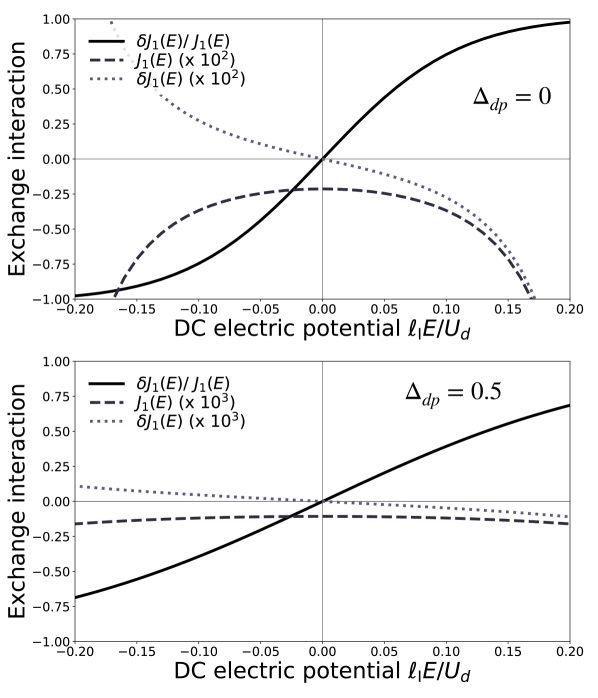
Figure 15: The $\bm{E}$-induced bond alternation $\delta J_{1}(\bm{E})$ is plotted for the DC electric potential $\ell_{\rm I}E$ for the $J_{1}<0<J_{2}$ case with parameters, $U_{d}=1$, $U_{p}=0.5$, $J_{H}=0.5$, $t=0.1$, $t^{\prime}=0.01$, and $\ell_{\rm II}/\ell_{\rm I}=0.81$. The ratio $\ell_{\rm II}/\ell_{\rm I}$ is determined from the data for $\mathrm{NaCuMoO_{4}(OH)}$ Nawa et al. (2015). We took $\Delta_{dp}=0$ for the upper panel and $\Delta_{dp}=0.5$ for the lower panel.

The dimer order parameter $D(\bm{E})$ characterizes the $\bm{E}$-induced dimer phase. When the ground state belongs to the TL-liquid phase for $\bm{E}=\bm{0}$, the dimer order parameter is obviously zero: $D(\bm{0})=0$. As soon as we apply the DC electric field to the TL liquid, we can open the excitation gap. The gap opening due to the bond alternation is well described by the sine-Gordon theory with the following Hamiltonian Giamarchi (2004).

$$\mathcal{H}_{\rm chain} \approx\frac{v}{2}\int dx\{(\partial_{x}\theta)^{2}+(\partial_{x}\phi)^{2}\}$$

$$\qquad+g(\bm{E})\int dx\,\cos(\sqrt{2\pi}\phi),$$ (50)

where $v$ is the spinon velocity and $g(\bm{E})\propto\delta J_{1}(\bm{E})\propto|E|$ is the coupling constant that leads to the spin gap. $\phi$ and $\theta$ are related to the spin operator $\bm{S}_{j}$ as Giamarchi (2004); Gogolin et al. (2004); Hikihara and Furusaki (2004)

$$S_{j}^{z} =\frac{1}{\sqrt{2\pi}}\partial_{x}\phi+(-1)^{j}a_{1}\cos(\sqrt{2\pi}\phi),$$ (51)

$$S_{j}^{+} =e^{-i\sqrt{2\pi}\theta}[b_{0}(-1)^{j}+b_{1}\cos(\sqrt{2\pi}\phi)],$$ (52)

with nonuniversal constants $a_{1}$, $b_{0}$, and $b_{1}$. It is exactly known that the sine-Gordon theory (50) gives the following the dimer order parameter $D(\bm{E})$ Lukyanov and Zamolodchikov (1997):

$$D(\bm{E}) =\frac{1}{L}\sum_{j=1}^{L}\braket{(-1)^{j}\bm{S}_{j}\cdot\bm{S}_{j+1}}$$

$$=3d_{z}\int dx\,\braket{\cos(\sqrt{2\pi}\phi)}$$

$$=3d_{z}\biggl{[}\frac{\Delta(\bm{E})\sqrt{\pi}\Gamma(2/3)}{v\Gamma(1/6)}\biggr{]}^{1/2}\exp\biggl{[}\int_{0}^{\infty}\frac{dt}{t}\biggl{\{}-\frac{1}{2}e^{-2t}$$

$$\qquad+\frac{\sinh^{2}(t/2)}{2\sinh(t/4)\sinh t\cosh(3t/4)}\biggr{\}}\biggr{]}.$$ (53)

where the parameter $d_{z}$ relates the spin operator and the $\phi$ boson via $(-1)^{j}S_{j}^{p}S_{j+1}^{p}=d_{z}\sin(\sqrt{2\pi}\phi)+\cdots$ for $p=x,y,z$ in the absence of the DC electric field Takayoshi and Sato (2010); Hikihara et al. (2017) and $\Gamma(z)$ is the gamma function. The parameter $\Delta(\bm{E})$ represents the lowest-energy excitation gap induced by $\bm{E}$. Note that $v$ and $d_{z}$ are calculated in the model with $\bm{E}=\bm{0}$ since the $\bm{E}$ dependence of these quantities merely leads to hardly observable corrections to the right hand side of Eq. (53), which we will discuss later. The field-theoretical result (53) becomes accurate when the ratio $J_{1}(\bm{0})/J_{2}(\bm{0})$ is close to the critical value $\alpha_{c}$. When $J_{1}(\bm{0})/J_{2}(\bm{0})\approx\alpha_{c}$, the parameters $v$ and $d_{z}$ are given by $v=1.174J_{1}(\bm{0})$ Okamoto and Nakamura (1997) and $d_{z}=0.182$ Takayoshi and Sato (2010).

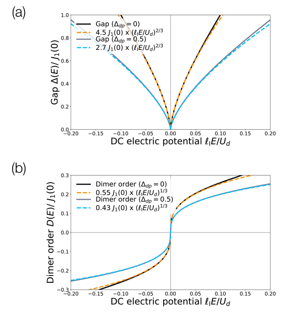
Figure 16: (a) The $\bm{E}$-induced excitation gap $\Delta(\bm{E})$ (54) (46) (solid lines) is plotted and compared with a simple power-law function $\propto(\ell_{\rm I}E/U_{d})^{2/3}$ (dashed lines). (b) The $\bm{E}$-induced dimer order parameter (53) (the solid lines) is plotted and compared with a simple power-law function $\propto(\ell_{\rm I}E/U_{d})^{1/3}$ (the dashed lines). We used the same parameters as those in Fig. 14.

One can obtain the exact excitation gap, $\Delta(\bm{E})$, of the sine-Gordon theory (50) Lukyanov and Zamolodchikov (1997); Lukyanov (1997); Zamolodchikov (1995):

$$\Delta(\bm{E}) =\frac{2v}{\sqrt{\pi}}\frac{\Gamma(1/6)}{\Gamma(2/3)}\biggl{(}\frac{3d_{z}\pi}{2}\frac{\Gamma(3/4)}{\Gamma(1/4)}\frac{|\delta J_{1}(\bm{E})|}{v}\biggr{)}^{2/3}$$

$$\propto\biggl{(}\frac{|\delta J_{1}(\bm{E})|}{J_{1}(\bm{0})}\biggr{)}^{2/3}.$$ (54)

Equation (49) tells us that the $\bm{E}$-induced bond alternation $\delta J_{1}(\bm{E})$ is proportional to $E$ for $|E|\ll(U_{d}-U_{p})/\ell_{\rm I}$. Therefore, we obtain

$$\Delta(\bm{E}) \propto|E|^{2/3},$$ (55)

$$D(\bm{E}) \propto|E|^{1/3}.$$ (56)

The gap (54) and the dimer order (53) are plotted in Fig. 16. We can see the power-law behaviors (55) and (56) near $\bm{E}=\bm{0}$. The power laws (55) and (56) hold near the origin but break down at some field strength, say, for $|\ell_{\rm I}E/U_{d}|\approx 0.1$ when $\Delta_{dp}=0$ (Fig. 16), because of a nonlinear $E$ dependence of $J_{1}(\bm{E})$ and $\delta J_{1}(\bm{E})$ [Eqs. (48) and (49)]. Since $U_{d}$ is typically $\sim 5~{}\mathrm{eV}$ for Cu Antonides et al. (1977); Yin et al. (1977); Fujimori et al. (1993), we can expect this nonlinear effect for $|E|\gtrsim 34~{}\mathrm{MV/cm}$, which is extremely strong. The nonlinear effect will be hardly observable. At the same time, this estimation of $|E|$ justifies our perturbative treatment of the DC electric field in the field-theoretical argument such as Eq. (53).

This $\bm{E}$-induced dimerization differs significantly from a magnetic-field-induced dimerization that one of the authors found recently Furuya (2020). Though a fourfold screw symmetry is essential to cause the magnetic-field-induced dimerization, such a complication is not required in the $\bm{E}$-induced dimerization.

V.4.2 $J_{1}<0$: Haldane dimers

When $J_{1}<0<J_{2}$, the ground-state phase diagram at $E=h=0$ contains the ferromagnetically ordered phase, a vector-chiral phase, and the Haldane-dimer phase Furukawa et al. (2012). When $0<J_{1}/J_{2}\ll 1$, the ground state is expected to belong to the Haldane-dimer phase, where the triplet dimer is formed on the nearest-neighbor bond. Reference Furukawa et al. (2012) also discusses the effects of the bond alternation on the ground-state phase diagram of the $J_{1}$–$J_{2}$ chain. The bond alternation weakens the geometrical frustration between the nearest-neighbor and the next-nearest-neighbor exchange interactions. While the $J_{1}$–$J_{2}$ spin chain with $J_{1}<0<J_{2}$ has the spontaneous Haldane-dimer phase with the twofold ground-state degeneracy, the $J_{1}$–$J_{2}$–$\delta J_{1}$ chain has the induced Haldane-dimer phase with the unique and gapped ground state. In the latter phase, the triplet dimer is formed on the bond with the stronger nearest-neighbor exchange interaction, namely, on the $J_{1}+\delta J_{1}$ bond for $E>0$ and on the $J_{1}-\delta J_{1}$ bond for $E<0$ [Fig. 13 (c3)].

Differently from the $J_{1}>0$ case, the DC electric field does not open the spin gap for large $|J_{1}|$. When $J_{1}<0$ and $|J_{1}|$ is large enough, the ground state has the spontaneous ferromagnetic order accompanied by a gapless nonrelativistic Nambu-Goldstone mode, which is robust against the small bond alternation. When $|J_{1}|$ is much smaller than $J_{2}$, the DC electric field opens the gap exactly in the same way for both the $J_{1}<0$ and $J_{1}>0$ cases.

When $\max\{|J_{1}|,|\delta J_{1}|\}\ll J_{2}$, we can regard the $J_{1}$–$J_{2}$ spin chain as weakly coupled spin chains. Bosonizing each spin chain, we obtain an excitation gap Shelton et al. (1996),

$$\Delta(\bm{E})\propto|\delta J_{1}(\bm{E})|\propto|E|,$$ (57)

instead of Eq. (54). Accordingly, the dimer order parameter follows

$$D(\bm{E})\approx|\delta J_{1}(\bm{E})|^{1/2}.$$ (58)

Therefore, we find for weak $E\ll(U_{d}-U_{p})/\ell_{\rm I}$ that

$$\Delta(\bm{E}) \propto|E|,$$ (59)

$$D(\bm{E}) \propto|E|^{1/2}.$$ (60)

Though we obtained different power laws from Eqs. (55) and (56), it is not attributed to the sign of $J_{1}$. In fact, even when $J_{1}>0$, we will find the power laws (59) and (60) if $J_{1}$ and $|\delta J_{1}|$ are much smaller than $J_{2}$. In this weak $|J_{1}|$ region, we can find the difference due to the sign of $J_{1}$ only in the nature of the dimer order whether it is the Haldane dimer or the singlet one.

V.5 Proposals for experiments

The following are our proposals for experiments. The CuO₂ chain of Fig. 13 is realized, for example, in $A\mathrm{CuMoO_{4}(OH)}$ ($A=\mathrm{Na,K}$) Nawa et al. (2015, 2014, 2017). $(J_{1},J_{2})$ are given by $(-51~{}\mathrm{K},\,36~{}\mathrm{K})$ for $A=\mathrm{Na}$ and $(238~{}\mathrm{K},\,0)$ for $A=\mathrm{K}$. We can expect the $\bm{E}$-induced dimerization for $A=\mathrm{K}$ and the $\bm{E}$-induced Haldane-dimer phase for $A=\mathrm{Na}$

For $A=\mathrm{K}$, it will be intriguing to observe the $2/3$-power-law dependence (55) of the excitation gap $\Delta(\bm{E})$. We expect that the DC electric field with $1~{}\mathrm{MV/cm}$ opens the gap $\sim 22~{}\mathrm{K}$ in $\mathrm{KCuMoO_{4}(OH)}$, which reaches $8.6~{}\%$ of $J_{1}(\bm{0})$. Spectroscopic methods such as the electron spin resonance (ESR) Zvyagin et al. (2004); Glazkov et al. (2010), the inelastic neutron scattering Nishi et al. (1994), and the Raman scattering Sato et al. (2012); Prosnikov et al. (2018) will be suitable candidates for observing those characteristics.

There is another interesting phenomenon specific to $\mathrm{KCuMoO_{4}(OH)}$. The compound $\mathrm{KCuMoO_{4}(OH)}$ has a staggered Dzyaloshinskii-Moriya (DM) interaction, $\sum_{j}(-1)^{j}\bm{D}\cdot\bm{S}_{j}\times\bm{S}_{j+1}$, in addition to the Hamiltonian (47). The DM interaction originates from the spin-orbit coupling. Though we did not take the spin-orbit coupling into account thus far in this paper, we can approximately apply our theory to this compound since the DM interaction is weak. As far as the leading effects caused by the perturbative DM interaction and the perturbative electric field are concerned, we can still adapt our theory to those systems with the weak DM interaction. If one wishes to discuss DC electric-field controls of DM interactions, one has to take into account the spin-orbit coupling in the electric models such as Eq. (2) and (5), which goes beyond the scope of this paper.

The staggered DM interaction yields a staggered magnetic-field interaction (say, $-h_{s}\sum_{j}(-1)^{j}S_{j}^{x}$) when the external DC magnetic field $h$ is applied in a direction perpendicular to $\bm{D}$ Oshikawa and Affleck (1997); Affleck and Oshikawa (1999).

The resultant staggered magnetic field is proportional to $h$ and $|\bm{D}|$: $h_{s}\propto|\bm{D}|h/J$. As well as the bond alternation $\delta J_{1}(\bm{E})$, the staggered magnetic field $h_{s}$ also generates the excitation gap. The staggered magnetic field induces the Néel order in a direction perpendicular to the external DC magnetic field Affleck and Oshikawa (1999). When the DC electric and magnetic fields are applied to the spin chain simultaneously and are tuned, a crossover will occur between the $\bm{E}$-induced dimerized phase and the $h_{s}$-induced Néel phase. The entanglement of the singlet dimer is protected by one of the time-reversal, the $D_{2}$ spin-rotation, and the bond-centered inversion symmetries Chen et al. (2011a, b); Nakagawa et al. (2018). All these symmetries are explicitly broken in the simultaneous presence of the DC electric and magnetic fields. Namely, nothing forbids the smooth deformation of the $E$-induced dimer-ordered ground state into the $H$-induced Néel ordered ground state. It will be interesting to look into whether the crossover actually occurs on the two-dimensional parameter space shown in Fig. 17.

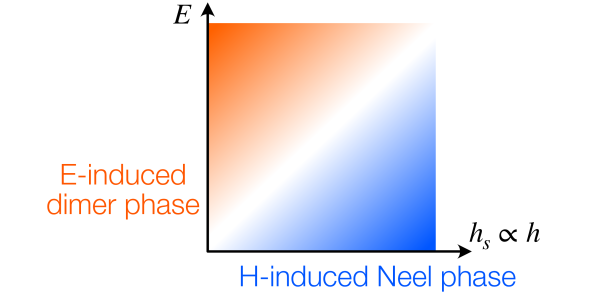
Figure 17: Possible $E$-$H$ ground-state phase diagram of $\mathrm{KCuMoO_{4}(OH)}$. When $E\not=0$ and $h_{s}=0$ $(=h)$, the $E$-induced singlet-dimer phase is realized. By contrast, when $E=0$ and $h_{s}\not=0$, the $h_{s}$-induced Néel phase is realized. These ground states will be smoothly connected to each other because the symmetries protecting these gapped quantum phases are explicitly broken.

Due to the staggered DM interaction, the field dependence of the excitation gap will be tractable in ESR measurements Sakai and Shiba (1994); Oshikawa and Affleck (1999); Furuya and Oshikawa (2012). One significant difference of these two phases lies in a localized excited state at the chain end, called the boundary bound state Furuya and Oshikawa (2012), exists only in the $h_{s}$-induced Néel phase Furuya and Oshikawa (2012). With an increase of $|E|$, the boundary bound state will be eventually lost though it will survive for a while in the vicinity of the horizontal axis of Fig. 17.

For $A=\mathrm{Na}$, the nearest-neighbor interaction is ferromagnetic. The ratio $J_{1}(\bm{0})/J_{2}(\bm{0})\approx-1.4$ implies that the ground state at zero magnetic field belongs to the Haldane-dimer phase (Fig. 1 of Ref. Furukawa et al. (2012)). Experimentally, DC electric-field effects on the Haldane-dimer phase can be observed as an increase of the excitation gap similarly to the $J_{1}>0$ case. We can also observe an $S=1/2$ edge state. The spin-1 Haldane phase is a topological phase protected by the $\mathbb{Z}_{2}\times\mathbb{Z}_{2}$ spin-rotation symmetry Pollmann et al. (2010, 2012). Since the DC electric fields keep the $\mathbb{Z}_{2}\times\mathbb{Z}_{2}$ symmetry, the $\bm{E}$-induced Haldane-dimer phase has doubly degenerate edge states on each chain end, that is, an $S=1/2$ edge spin. The edge-spin degrees of freedom can be observed by, for example, the ESR spectroscopy Hagiwara et al. (1990); Yoshida et al. (2005). An increase in the excitation gap immediately means a decrease in the correlation length. The decrease of the correlation length would affect the ESR spectrum of the spin chain with a finite chain length Yoshida et al. (2005).

VI Other DC electric-field effects

This section is devoted to discussions on other major DC electric-field effects that we have not dealt with in this paper. We can incorporate some effects into our model with slight modifications and some with substantial changes. The renormalization of the dielectric constant and the structural distortion fall into the former. The spin-orbit coupling falls into the latter and requires the substantial change of the model. In what follows, we briefly discuss these three effects and another important effect of the THz laser pulse.

VI.1 Dielectric constant

We implicitly assumed that the electrons feel the external DC electric field itself. In real materials, the electron is surrounded by various charges that can screen or enhance the external electric field. Generally, the dielectric function represents how the external DC electric field is screened or enhanced. In particular, the dielectric constant in the material gets shifted from its vacuum value. We can incorporate this effect into our model by regarding $\bm{E}(\bm{r})$ in our model as the actual DC electric field that the electrons in materials actually feel.

VI.2 Structural distortion

The strong DC electric field can possibly distort the crystal structure. Still, the $\bm{E}$-induced change of the on-site potential $V_{j}$ turns out to be dominant, as shown below. The structural distortion will make the hopping amplitude $t_{j}$ depend on $\bm{E}$ by modifying the lattice spacing. We did not include this effect in our analysis thus far but can immediately include it without any problem. Namely, we just replace the constant $t_{j}$ by an $\bm{E}$-dependent function $t_{j}(\bm{E})$. If one wishes to predict the precise $\bm{E}$ dependence of the hopping amplitude, one needs to model how the DC electric field distorts the lattice.

Besides, the structural distortion can lower the crystalline symmetry. The symmetry lowering leads to an important effect of switching on hoppings between $d$ and $p$ orbitals that were forbidden by symmetries in the absence of the DC electric field. Then, we need to include $d$- or $p$-orbital degeneracy explicitly into the model Hamiltonian. However, since such a newly introduced hopping amplitude is proportional to the DC electric-field strength, the inclusion of the degenerate $d$ or $p$ orbitals will become important only under extremely strong DC electric fields. Let us denote the additional hopping amplitude as $t^{\prime}_{j}(\bm{E})$ for $j=0,1$. Note that $t^{\prime}_{j}(\bm{0})=0$ by definition. It is straightforward to include $t^{\prime}$ into our results. We can obtain the correction by $t^{\prime}_{j}(\bm{E})$ to Eqs. (17) and (20) by replacing $t_{j}$ in these relations to $t^{\prime}_{j}$ totally or partially. The fourth-order perturbation expansion shows that this correction to the superexchange coupling is an even order of $\ell|\bm{E}|/U_{d}$ because an electron in a $p$ orbital hopped to a $d$ orbital must come back to the same $p$ orbital from the same $d$ orbital in the Mott-insulating phase. $t^{\prime}_{j}(\bm{E})$ gives corrections of $O((t^{\prime}_{j}(\bm{E})/U_{d})^{4})\leq O((\ell|\bm{E}|/U_{d})^{4})$ to Eq. (17), that is, fourth order about the DC electric field. On the other hand, $t^{\prime}_{j}(\bm{E})$ gives corrections of $O((t^{\prime}_{j}(\bm{E})/U_{d})^{2})\leq O((\ell|\bm{E}|/U_{d})^{2})$ to Eq. (20). In any case, the correction is nonlinear about the DC electric field.

As we saw throughout the paper, the strong DC electric field of $O(1)$ MV/cm is already required to change the superexchange interaction by a few percent. Accordingly, we need much stronger DC electric field to observe the nonlinear change of the superexchange. Under such situations, the second- or fourth-order effect will be relevant only for $O(10)$ MV/cm for inorganic materials and for $O(1)$ MV/cm for organic ones. There will be a chance in organic materials to observe the nonlinear field effects including that by the symmetry-lowering structural distortion. However, it will be difficult to distinguish the structural distortion effect from other nonlinear terms in Eqs. (17) and (20). Therefore, the inclusion of the structural distortion keeps our result intact unless the subleading nonlinear field effects are concerned.

Finally, we comment on a possible spontaneous formation of the electric polarization due to the $\bm{E}$-driven structural phase transition. Such a spontaneous polarization can become large even if $\ell|\bm{E}|/U_{d}\ll 1$. This large polarization can potentially lead to a large correction to the superexchange coupling. It will be interesting in the future to investigate such $\bm{E}$-driven phase-transition effects.

VI.3 Spin-orbit coupling

The spin-orbit coupling can dramatically change the spin Hamiltonian by adding to the spin Hamiltonian anisotropic interactions such as the DM interaction. It needs straightforward but lengthy calculations to discuss the effects of the spin-orbit coupling on electric-field controls of magnetism Furuya and Sato . We will discuss in a subsequent paper Furuya and Sato the combination effect of the spin-orbit coupling and the DC electric field.

VI.4 THz laser pulse

The single-cycle THz laser pulse can be deemed the effective DC electric field when the relevant time scale of the spin system is fast enough. We need this assumption of the fast spin dynamics to guarantee that the quantum spin system quickly reaches the equilibrium before the pulse laser disappears. The typical time scale ranges from $\sim 0.1$ ps to $\sim 1$ ns Kirilyuk et al. (2010); Oshikawa and Affleck (2002); Furuya and Sato (2015); Beaurepaire et al. (1996); Koopmans et al. (2000); Mashkovich et al. (2019); Tzschaschel et al. (2019); Lenz et al. (2006); Vittoria et al. (2010). For example, the spin dynamics with the time scale $\sim 0.1-1$ ps is much faster than the single cycle ($\sim 10$ ps) of the THz laser pulse with the $0.1$ THz frequency Hirori et al. (2011); Mukai et al. (2016); Nicoletti and Cavalleri (2016). Then, we can regard the single-cycle THz laser pulse as the effective DC electric field. On the other hand, if we apply the laser pulse with the $10$ THz frequency to the spin system with the time scale $\gtrsim 10$ ps, the pulse ($\sim 0.1$ ps) disappears much faster than the equilibration of the spin system. Then, the single-cycle THz laser pulse can be approximated as a delta-function electric field, $\bm{E}(t)=\bm{E}_{0}\delta(t)$. Even when the spin dynamics is much slower than the THz laser pulse width, the electron dynamics can be much faster than the pulse width. Indeed, the hopping amplitude $t\sim O(1)$ eV gives the time scale $O(1)~{}\mathrm{fs}=O(10^{-3})~{}\mathrm{ps}$. Therefore, we can incorporate the THz laser pulse as an effective DC electric field into our model even when the pulse width is too short to equilibrate the spin system. We then notice an interesting possibility. If we derive the effective spin model, the THz laser pulse turns into the delta-function potential, $\delta J(\bm{E}_{0})\delta(t)$, that instantaneously modifies the exchange interaction at the time $t=0$. It is an interesting direction of future studies to investigate dynamical effects caused by the instantaneous potential.

To conclude, we emphasize two points. The THz laser pulse can be deemed the effective DC electric field. The THz laser pulse can equilibrate the spin system and otherwise induces the instantaneous modification of the exchange interaction, which depends on materials.

VII Summary

This paper discussed DC electric-field controls of superexchange interactions in Mott insulators. We first presented the generic results (17) and (20) about the superexchange interaction by the fourth-order degenerate perturbation expansion of the two basic electron models. We considered the antiferromagnetic and ferromagnetic superexchange interactions and obtained their $\bm{E}$ dependence.

The other part of the main text was devoted to applications of the generic results to basic geometrically frustrated quantum spin systems. While the results of Sec. III applies to various quantum spin systems regardless of the lattice and the dimensionality, we give our attention to low-dimensional quantum spin systems in this application part to investigate how DC electric fields applied perpendicular to the system control the superexchange interactions without interfering with the spatial anisotropy. In contrast to this paper, the previous paper Takasan and Sato (2019) discussed how to control the “direct superexchange” interaction Note (1) and introduce the spatial anistoropy to the system through the DC electric field parallel to the system. These two theories complement each other.

As the first application, we considered $J_{1}$–$J_{2}$ frustrated quantum spin systems on the square lattice in Sec. IV. We first demonstrated in the toy model how the DC electric field adjusts the parameter $J_{1}(\bm{E})/J_{2}(\bm{E})$ that determines the fate of the ground state. Next, we applied the generic results of Sec. III to the more realistic model that emulates two compounds $\mathrm{BaCdVO(PO_{4})_{2}{}}$ Nath et al. (2008) and $A\mathrm{MoOPO_{4}Cl}{}$ Ishikawa et al. (2017). Combined to their crystal structures, the DC electric field breaks the inversion symmetry that introduces the nonequivalence of the next-nearest-neighbor interactions, $J_{2}(\bm{E})\pm\delta J_{2}(\bm{E})$ though the original model exactly has $\delta J_{2}(\bm{0})=0$ at $\bm{E}=\bm{0}$. An increase of the nonequivalence by $\delta J_{2}(\bm{E})$ turns the frustrated square-lattice quantum antiferromagnet eventually into the deformed triangular-lattice antiferromagnet, which will offer a unique experimental method to change the lattice structure effectively.

We also discussed applications to geometrically frustrated one-dimensional quantum spin systems, the $J_{1}$–$J_{2}$ spin chains. We assumed that there are two oxygen sites between the two nearest-neighbor magnetic ion sites, such as the CuO₂ chain. When two oxygen sites feel different electric potentials, the DC electric field breaks the one-site translation symmetry down to the two-site one. In other words, the number of spins per unit cell is doubled. The DC electric field then yields the bond alternation $\delta J_{1}(\bm{E})\sum_{j}(-1)^{j}\bm{S}_{j}\cdot\bm{S}_{j+1}$ while $\delta J_{1}(\bm{0})=0$. The appearance of the bond alternation drives the quantum critical phase of the spin chain into a unique gapped quantum phase with a dimerization, which is the first proposal of the DC electric-field-induced dimerization.

The $\bm{E}$-induced dimer phase is the singlet-dimer one for $J_{1}>0$ or the Haldane-dimer (triplet-dimer) one for $J_{1}<0$. The $\bm{E}$ dependence of the excitation gap will be experimentally visible in, for example, the ESR, the inelastic neutron scattering, and the Raman scattering experiments, which give evidence of the growth of the $E$-induced dimer orders.

We also briefly investigated other major DC electric-field effects that were not incorporated in our analyses. We hope that this paper stimulates further theoretical and experimental studies on electric-field controls of quantum magnetism.

Appendix A Fourth-order degenerate perturbations

This appendix is devoted to derivations of the generic formulas(17) and (20) of the superexchange coupling.

A.1 Antiferromagnetic superexchange interaction

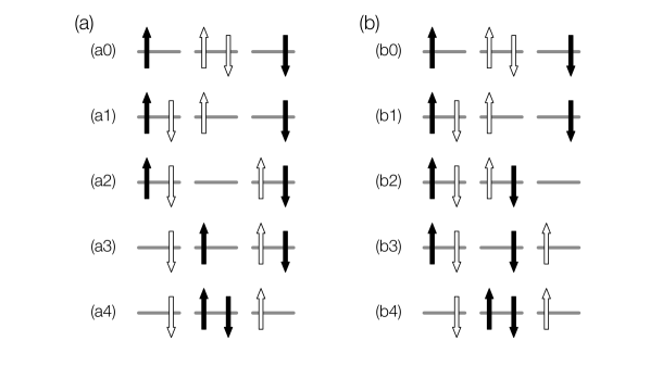
Figure 18: Two typical fourth-order processes, (a) and (b), of the perturbative expansion for the model (2). Filled (empty) arrows represent electron spins at $d$ ($p$, respectively) orbitals in the initial state (a0). (a0) and (a4) are initial and final states of the process (a) in Eq. (14), respectively. (a1), (a2), (a3) are intermediate ones. Applying the perturbation $\mathcal{H}_{t}$ to the state of (a$n$), we obtain the state of (a($n+1$)). The same rules apply to the process (b).

There are two kinds of processes that have nontrivial contributions to the fourth-order term $\mathcal{H}_{4}^{\rm eff}$ of Eq. (14). Figure 18 depicts two representatives of the fourth-order perturbation processes. While the $p$ orbitals are temporally empty in the process (a), one of the $p$ orbitals are always filled in the process (b). Every fourth-order process fits into either the process (a) or the process (b) with minor differences of the spin orientation. All we have to do is to complete the calculations of the processes (a) and (b) with generic spin orientations.

Let us denote contributions of those processes as

$$\mathcal{H}_{4}^{\rm eff} =\mathcal{H}_{4}^{\rm eff;a}+\mathcal{H}_{4}^{\rm eff;b}.$$ (61)

The contribution from the process (a) exemplified by Fig. 18 (a) is the following.

$$\mathcal{H}_{4}^{\rm eff;a} =-P\biggl{(}\frac{t_{0}^{\ast}t_{1}^{\ast}}{\Delta_{1}+U_{d}-U_{p}}\sum_{\sigma^{\prime}}p_{\frac{1}{2},-\sigma^{\prime}}^{\dagger}d_{1,-\sigma^{\prime}}p_{\frac{1}{2},\sigma^{\prime}}^{\dagger}d_{0,\sigma^{\prime}}+\frac{t_{1}^{\ast}t_{0}^{\ast}}{\Delta_{0}+U_{d}-U_{p}}\sum_{\sigma^{\prime}}p_{\frac{1}{2},-\sigma^{\prime}}^{\dagger}d_{0,-\sigma^{\prime}}p_{\frac{1}{2},\sigma^{\prime}}^{\dagger}d_{1,\sigma^{\prime}}\biggr{)}$$

$$\quad\cdot\biggl{(}\frac{t_{1}t_{0}}{(\Delta_{0}+\Delta_{1}+2U_{d}-U_{p})(\Delta_{0}+U_{d}-U_{p})}\sum_{\sigma}d_{1,-\sigma}^{\dagger}p_{\frac{1}{2},-\sigma}d_{0,\sigma}^{\dagger}p_{\frac{1}{2},\sigma}$$

$$\qquad+\frac{t_{0}t_{1}}{(\Delta_{0}+\Delta_{1}+2U_{d}-U_{p})(\Delta_{1}+U_{d}-U_{p})}\sum_{\sigma}d_{0,-\sigma}^{\dagger}p_{\frac{1}{2},-\sigma}d_{1,\sigma}^{\dagger}p_{\frac{1}{2},\sigma}\biggr{)}P.$$ (62)

Since the $p$ orbitals are fully occupied within the subspace spanned by the unperturbed ground state, the projection $P$ onto this subspace enables us to remove operators of the $p$ orbitals:

$$Pp_{\frac{1}{2},-\sigma^{\prime}}^{\dagger}p_{\frac{1}{2},\sigma^{\prime}}^{\dagger}p_{\frac{1}{2},-\sigma}p_{\frac{1}{2},\sigma}P =\delta_{\sigma^{\prime},\sigma}-\delta_{\sigma^{\prime},-\sigma}.$$ (63)

In addition, some products of operators at $d$ orbitals are rewritten in terms of the $S=1/2$ spin operators $\bm{S}_{j}=\frac{1}{2}\sum_{\sigma,\sigma^{\prime}}d_{j,\sigma}^{\dagger}\bm{\sigma}^{\sigma\sigma^{\prime}}d_{j,\sigma^{\prime}}$. The contribution (62) of the process (a) is thus reduced to a simple form,

$$\mathcal{H}_{4}^{\rm eff;a} =P\biggl{[}2|t_{0}t_{1}|^{2}\biggl{(}\frac{1}{\Delta_{0}+U_{d}-U_{p}}+\frac{1}{\Delta_{1}+U_{d}-U_{p}}\biggr{)}^{2}\frac{1}{\Delta_{0}+\Delta_{1}+2U_{d}-U_{p}}\bm{S}_{0}\cdot\bm{S}_{1}+\mathrm{const.}\biggr{]}P.$$ (64)

We can obtain $\mathcal{H}_{4}^{\rm eff;b}$ similarly:

$$\mathcal{H}_{4}^{\rm eff;b} =-P\biggl{(}\frac{t_{0}^{\ast}t_{1}}{\Delta_{0}+U_{d}-U_{p}}\sum_{\sigma^{\prime}}p_{\frac{1}{2},\sigma^{\prime}}^{\dagger}d_{0,\sigma^{\prime}}d_{1,\sigma^{\prime}}^{\dagger}p_{\frac{1}{2},\sigma^{\prime}}\frac{t_{1}^{\ast}t_{0}}{(\Delta_{1}-\Delta_{0}+U_{d})(\Delta_{0}+U_{d}-U_{p})}\sum_{\sigma}p_{\frac{1}{2},\sigma}^{\dagger}d_{1,\sigma}d_{0,\sigma}^{\dagger}p_{\frac{1}{2},\sigma}$$

$$\qquad+\frac{t_{t}^{\ast}t_{0}}{\Delta_{1}+U_{d}-U_{p}}\sum_{\sigma^{\prime}}p_{\frac{1}{2},\sigma^{\prime}}^{\dagger}d_{1,\sigma^{\prime}}d_{0,\sigma^{\prime}}^{\dagger}p_{\frac{1}{2},\sigma^{\prime}}\frac{t_{0}^{\ast}t_{1}}{(\Delta_{0}-\Delta_{1}+U_{d})(\Delta_{1}+U_{d}-U_{p})}\sum_{\sigma}p_{\frac{1}{2},\sigma}^{\dagger}d_{0,\sigma}d_{1,\sigma}^{\dagger}p_{\frac{1}{2},\sigma}\biggr{)}P$$

$$=P\biggl{[}2|t_{0}t_{1}|^{2}\biggl{(}\frac{1}{(\Delta_{0}+U_{d}-U_{p})^{2}}\frac{1}{\Delta_{0}-\Delta_{1}+U_{d}}+\frac{1}{(\Delta_{1}+U_{d}-U_{p})^{2}}\frac{1}{\Delta_{1}-\Delta_{0}+U_{d}}\biggr{)}\bm{S}_{0}\cdot\bm{S}_{1}+\mathrm{const.}\biggr{]}P.$$ (65)

Combining Eqs. (64) and (65), we reach the final result of the antiferromagnetic superexchange coupling (17), which is consistent with the special case of $\Delta_{0}=\Delta_{1}$ and $t_{0}=t_{1}\in\mathbb{R}$ Koch (2012).

A.2 Ferromagnetic superexchange interaction

The ferromagnetic superexchange coupling (20) is similarly derived. Two processes contribute to the fourth-order term (14) as shown in Fig. 19. The process (a) of Fig. 19 exchanges spins at $j=0$ and $j=1$ sites. On the other hand, the process (b) of Fig. 19 does not. Nevertheless, the latter must be taken into account because it gives rise to a term $S_{0}^{z}S_{1}^{z}$, as we will see soon.

A major difference of the present model (5) from the previously dealt one (2) comes from the Coulomb exchange (the ferromagnetic direct exchange), $J_{\rm H}$, that reconstructs the unperturbed eigenstates of the degenerate $p$ orbitals only when they are half occupied. We assumed the presence of two degenerate $p$ orbitals $p_{x}$ and $p_{y}$. Without the hopping terms, the eigenstates are given by a product state $\ket{\phi_{d}}\ket{\phi_{p}}$, where $\ket{\phi_{\mu}}$ denotes the eigenstate at the $\mu=d,p$ orbital. $\ket{\phi_{d}}$ is further split into a product of local states at two $d$-orbital sites. The same applies to $\ket{\phi_{p}}$ except for the case mentioned above. When the $p$ orbitals are half occupied, their eigenstates are reconstructed as the singlet $\ket{\phi_{p}}=(\ket{\uparrow_{x}\downarrow_{y}}-\ket{\downarrow_{x}\uparrow_{y}})/\sqrt{2}$ and triplets, $\ket{\phi_{p}}=\ket{\uparrow_{x}\downarrow_{y}}$, $(\ket{\uparrow_{x}\downarrow_{y}}+\ket{\downarrow_{x}\uparrow_{y}})/\sqrt{2}$, and $\ket{\downarrow_{x}\downarrow_{y}}$. Here, $\ket{\sigma_{x}\sigma_{y}}$ denotes the eigenstate of the $p$ orbitals. Note that the triplets have the eigenenergy lower than the singlet by $2J_{\rm H}$ ($>0$).

Paying attention to the reconstruction of $p$ orbitals, we can calculate the fourth-order term (14). Let us inherit the notation of Eq. (61). Here, the processes (a) and (b) are replaced by those of Fig. 19. The process (a) of Fig. 19 leads to

Figure 19: Two typical fourth-order processes, (a) and (b), of the perturbative expansion for the model (5), similarly drawn to Fig. 18. The red rounded square represents a reconstruction of the $p$-orbital eigenstates by the Coulomb exchange $J_{\rm H}$ [cf. Fig. 4 (b)]. The $p$-orbital states surrounded by this curve is either symmetrized or antisymmetrized. The former corresponds to one of the triplet states and the latter to the singlet state. This reconstruction permits hoppings, for instance, from the $j=0$ site to the $y$ orbital at the $j=1/2$ site, that were forbidden for $J_{\rm H}=0$.

$$\mathcal{H}_{4}^{\rm eff;a} =-P\biggl{(}\frac{t_{1}^{\ast}t_{0}^{\ast}}{\Delta_{1}+U_{d}-U_{p}}\sum_{\sigma^{\prime}}p_{\frac{1}{2},-\sigma^{\prime},y}^{\dagger}d_{1,-\sigma^{\prime}}p_{\frac{1}{2},\sigma^{\prime},x}^{\dagger}d_{0,\sigma^{\prime}}+\frac{t_{0}^{\ast}t_{1}^{\ast}}{\Delta_{0}+U_{d}-U_{p}}\sum_{\sigma^{\prime}}p_{\frac{1}{2},-\sigma^{\prime},x}^{\dagger}d_{0,-\sigma^{\prime}}p_{\frac{1}{2},\sigma^{\prime},y}^{\dagger}d_{1,\sigma^{\prime}}\biggr{)}$$

$$\quad\cdot\biggr{[}\frac{1}{2}\biggl{(}\frac{t_{1}}{\Delta_{0}+\Delta_{1}+2(U_{d}-U_{p})+J_{\rm H}}+\frac{t_{1}}{\Delta_{0}+\Delta_{1}+2(U_{d}-U_{p})-J_{\rm H}}\biggr{)}\frac{t_{0}}{\Delta_{0}+U_{d}-U_{p}}\sum_{\sigma}d_{1,-\sigma}^{\dagger}p_{\frac{1}{2},-\sigma,y}d_{0,\sigma}^{\dagger}p_{\frac{1}{2},\sigma}$$

$$\quad+\frac{1}{2}\biggl{(}\frac{t_{0}}{\Delta_{0}+\Delta_{1}+2(U_{d}-U_{p})+J_{\rm H}}+\frac{t_{0}}{\Delta_{0}+\Delta_{1}+2(U_{d}-U_{p})-J_{\rm H}}\biggr{)}\frac{t_{1}}{\Delta_{1}+U_{d}-U_{p}}\sum_{\sigma}d_{0,\sigma}^{\dagger}p_{\frac{1}{2},-\sigma,x}d_{1,\sigma}^{\dagger}p_{\frac{1}{2},\sigma,y}$$

$$\quad+\frac{1}{2}\biggl{(}\frac{t_{1}}{\Delta_{0}+\Delta_{1}+2(U_{d}-U_{p})+J_{\rm H}}-\frac{t_{1}}{\Delta_{0}+\Delta_{1}+2(U_{d}-U_{p})-J_{\rm H}}\biggr{)}\frac{t_{0}}{\Delta_{0}+U_{d}-U_{p}}\sum_{\sigma}d_{1,-\sigma}^{\dagger}p_{\frac{1}{2},\sigma,y}d_{0,\sigma}^{\dagger}p_{\frac{1}{2},-\sigma,x}$$

$$\quad+\frac{1}{2}\biggl{(}\frac{t_{0}}{\Delta_{0}+\Delta_{1}+2(U_{d}-U_{p})+J_{\rm H}}-\frac{t_{0}}{\Delta_{0}+\Delta_{1}+2(U_{d}-U_{p})-J_{\rm H}}\biggr{)}\frac{t_{1}}{\Delta_{1}+U_{d}-U_{p}}\sum_{\sigma}d_{0,-\sigma}^{\dagger}p_{\frac{1}{2},\sigma,x}d_{1,\sigma}^{\dagger}p_{\frac{1}{2},-\sigma,y}\biggr{]}P.$$ (66)

The last two terms represent spin-dependent hoppings that appear as a direct consequence of nonzero $J_{\rm H}$. They vanish in the $J_{\rm H}\to 0$ limit. Discarding the $p$ operators and translating the $d$ operators into spin operators with the aid of the projection $P$, we obtain

$$\mathcal{H}_{4}^{\rm eff;a} =P\biggl{[}|t_{0}t_{1}|^{2}\biggl{(}\frac{1}{\Delta_{0}+U_{d}-U_{p}}+\frac{1}{\Delta_{1}+U_{d}-U_{p}}\biggr{)}^{2}\frac{\Delta_{0}+\Delta_{1}+2(U_{d}-U_{p})}{[\Delta_{0}+\Delta_{1}+2(U_{d}-U_{p})]^{2}-{J_{\rm H}}^{2}}(1+2S_{0}^{z}S_{1}^{z})$$

$$\qquad-|t_{0}t_{1}|^{2}\biggl{(}\frac{1}{\Delta_{0}+U_{d}-U_{p}}+\frac{1}{\Delta_{1}+U_{d}-U_{p}}\biggr{)}^{2}\frac{J_{\rm H}}{[\Delta_{0}+\Delta_{1}+2(U_{d}-U_{p})]^{2}-{J_{\rm H}}^{2}}(S_{0}^{+}S_{1}^{-}+S_{0}^{-}S_{1}^{+})\biggr{]}P$$

$$=P\biggl{[}-2|t_{0}t_{1}|^{2}\biggl{(}\frac{1}{\Delta_{0}+U_{d}-U_{p}}+\frac{1}{\Delta_{1}+U_{d}-U_{p}}\biggr{)}^{2}\frac{J_{\rm H}}{[\Delta_{0}+\Delta_{1}+2(U_{d}-U_{p})]^{2}-{J_{\rm H}}^{2}}\bm{S}_{0}\cdot\bm{S}_{1}$$

$$\qquad+2|t_{0}t_{1}|^{2}\biggl{(}\frac{1}{\Delta_{0}+U_{d}-U_{p}}+\frac{1}{\Delta_{1}+U_{d}-U_{p}}\biggr{)}^{2}\frac{1}{\Delta_{0}+\Delta_{1}+2(U_{d}-U_{p})-J_{\rm H}}S_{0}^{z}S_{1}^{z}+\mathrm{const.}\biggr{]}P.$$ (67)

Eq. (67) turns out to break the $\mathrm{SU(2)}$ spin-rotation symmetry that the model possesses. The process (b) yields a compensating $S_{0}^{z}S_{1}^{z}$ term and restores the $\mathrm{SU(2)}$ spin-rotation symmetry. The process (b) leads to

$$\mathcal{H}_{4}^{\rm eff;b} =-P\biggl{(}\frac{t_{1}^{\ast}t_{0}^{\ast}}{\Delta_{1}+U_{d}-U_{p}}\sum_{\sigma^{\prime}}p_{\frac{1}{2},\sigma^{\prime},y}^{\dagger}d_{1,\sigma^{\prime}}p_{\frac{1}{2},\sigma^{\prime},x}^{\dagger}d_{0,\sigma^{\prime}}+\frac{t_{0}^{\ast}t_{1}^{\ast}}{\Delta_{0}+U_{d}-U_{p}}\sum_{\sigma^{\prime}}p_{\frac{1}{2},\sigma^{\prime},x}^{\dagger}d_{0,\sigma^{\prime}}p_{\frac{1}{2},\sigma^{\prime},y}^{\dagger}d_{1,\sigma^{\prime}}\biggr{)}$$

$$\qquad\cdot\biggl{(}\frac{t_{1}}{\Delta_{0}+\Delta_{1}+2(U_{d}-U_{p})-J_{\rm H}}\frac{t_{0}}{\Delta_{0}+U_{d}-U_{p}}\sum_{\sigma}d_{1,\sigma}^{\dagger}p_{\frac{1}{2},\sigma,y}d_{0,\sigma}^{\dagger}p_{\frac{1}{2},\sigma,x}$$

$$\qquad+\frac{t_{0}}{\Delta_{0}+\Delta_{1}+2(U_{d}-U_{p})-J_{\rm H}}\frac{t_{1}}{\Delta_{1}+U_{d}-U_{p}}\sum_{\sigma}d_{0,\sigma}^{\dagger}p_{\frac{1}{2},\sigma,x}d_{1,\sigma}^{\dagger}p_{\frac{1}{2},\sigma,y}\biggr{)}P$$

$$=P\biggl{[}-2|t_{0}t_{1}|^{2}\biggl{(}\frac{1}{\Delta_{0}+U_{d}-U_{p}}+\frac{1}{\Delta_{1}+U_{d}-U_{p}}\biggr{)}^{2}\frac{1}{\Delta_{0}+\Delta_{1}+2(U_{d}-U_{p})-J_{\rm H}}S_{0}^{z}S_{1}^{z}+\mathrm{const.}\biggr{]}P.$$ (68)

The last line of Eq. (68) indeed cancels the anisotropic term of Eq. (67). We thus end up with the isotropic ferromagnetic exchange coupling (20).

References

- Anderson (1973) P.W. Anderson, “Resonating valence bonds: A new kind of insulator?” Materials Research Bulletin 8, 153 – 160 (1973).
- Savary and Balents (2016) Lucile Savary and Leon Balents, “Quantum spin liquids: a review,” Reports on Progress in Physics 80, 016502 (2016).
- Zhou et al. (2017) Yi Zhou, Kazushi Kanoda, and Tai-Kai Ng, “Quantum spin liquid states,” Rev. Mod. Phys. 89, 025003 (2017).
- Knolle and Moessner (2019) J. Knolle and R. Moessner, “A Field Guide to Spin Liquids,” Annual Review of Condensed Matter Physics 10, 451–472 (2019).
- Jiang et al. (2012) Hong-Chen Jiang, Hong Yao, and Leon Balents, “Spin liquid ground state of the spin- square - Heisenberg model,” Phys. Rev. B 86, 024424 (2012).
- Metavitsiadis et al. (2014) Alexandros Metavitsiadis, Daniel Sellmann, and Sebastian Eggert, “Spin-liquid versus dimer phases in an anisotropic - frustrated square antiferromagnet,” Phys. Rev. B 89, 241104 (2014).
- Chubukov (1991) Andrey V. Chubukov, “Chiral, nematic, and dimer states in quantum spin chains,” Phys. Rev. B 44, 4693–4696 (1991).
- Shannon et al. (2006) Nic Shannon, Tsutomu Momoi, and Philippe Sindzingre, “Nematic Order in Square Lattice Frustrated Ferromagnets,” Phys. Rev. Lett. 96, 027213 (2006).
- Läuchli et al. (2006) Andreas Läuchli, Frédéric Mila, and Karlo Penc, “Quadrupolar Phases of the Bilinear-Biquadratic Heisenberg Model on the Triangular Lattice,” Phys. Rev. Lett. 97, 087205 (2006).
- Hikihara et al. (2008) Toshiya Hikihara, Lars Kecke, Tsutomu Momoi, and Akira Furusaki, “Vector chiral and multipolar orders in the spin- frustrated ferromagnetic chain in magnetic field,” Phys. Rev. B 78, 144404 (2008).
- Sudan et al. (2009) Julien Sudan, Andreas Lüscher, and Andreas M. Läuchli, “Emergent multipolar spin correlations in a fluctuating spiral: The frustrated ferromagnetic spin- Heisenberg chain in a magnetic field,” Phys. Rev. B 80, 140402 (2009).
- Penc and L’́auchli (2011) K. Penc and A. M. L’́auchli, Introduction to frustrated magnetism: materials, experiments, theory, Vol. 164 (Springer, Berlin, 2011) p. 331.
- Giamarchi et al. (2008) Thierry Giamarchi, Christian Rüegg, and Oleg Tchernyshyov, “Bose–Einstein condensation in magnetic insulators,” Nature Physics 4, 198–204 (2008).
- Zayed et al. (2017) ME Zayed, Ch Rüegg, AM Läuchli, C Panagopoulos, SS Saxena, M Ellerby, DF McMorrow, Th Strässle, S Klotz, G Hamel, et al., “4-spin plaquette singlet state in the Shastry–Sutherland compound SrCu2(BO3)2,” Nature physics 13, 962–966 (2017).
- Sakurai et al. (2018) Takahiro Sakurai, Yuki Hirao, Keigo Hijii, Susumu Okubo, Hitoshi Ohta, Yoshiya Uwatoko, Kazutaka Kudo, and Yoji Koike, “Direct observation of the quantum phase transition of SrCu2(BO3)2 by high-pressure and terahertz electron spin resonance,” Journal of the Physical Society of Japan 87, 033701 (2018).
- Zvyagin et al. (2019) SA Zvyagin, D Graf, T Sakurai, S Kimura, H Nojiri, J Wosnitza, H Ohta, T Ono, and H Tanaka, “Pressure-tuning the quantum spin Hamiltonian of the triangular lattice antiferromagnet Cs2CuCl4,” Nature communications 10, 1064 (2019).
- Oka and Aoki (2009) Takashi Oka and Hideo Aoki, “Photovoltaic Hall effect in graphene,” Phys. Rev. B 79, 081406 (2009).
- Kitagawa et al. (2011) Takuya Kitagawa, Takashi Oka, Arne Brataas, Liang Fu, and Eugene Demler, “Transport properties of nonequilibrium systems under the application of light: Photoinduced quantum hall insulators without landau levels,” Phys. Rev. B 84, 235108 (2011).
- Wang et al. (2013) Y. H. Wang, H. Steinberg, P. Jarillo-Herrero, and N. Gedik, “Observation of Floquet-Bloch States on the Surface of a Topological Insulator,” Science 342, 453–457 (2013).
- Jotzu et al. (2014) Gregor Jotzu, Michael Messer, Rémi Desbuquois, Martin Lebrat, Thomas Uehlinger, Daniel Greif, and Tilman Esslinger, “Experimental realization of the topological Haldane model with ultracold fermions,” Nature 515, 237–240 (2014).
- Shirley (1965) Jon H. Shirley, “Solution of the Schrödinger Equation with a Hamiltonian Periodic in Time,” Phys. Rev. 138, B979–B987 (1965).
- Sambe (1973) Hideo Sambe, “Steady States and Quasienergies of a Quantum-Mechanical System in an Oscillating Field,” Phys. Rev. A 7, 2203–2213 (1973).
- Bukov et al. (2015) Marin Bukov, Luca D’Alessio, and Anatoli Polkovnikov, “Universal high-frequency behavior of periodically driven systems: from dynamical stabilization to floquet engineering,” Advances in Physics 64, 139–226 (2015).
- Eckardt (2017) André Eckardt, “Colloquium: Atomic quantum gases in periodically driven optical lattices,” Rev. Mod. Phys. 89, 011004 (2017).
- Oka and Kitamura (2019) Takashi Oka and Sota Kitamura, “Floquet engineering of quantum materials,” Annual Review of Condensed Matter Physics 10, 387–408 (2019).
- Sato (2021) Masahiro Sato, “Floquet theory and ultrafast control of magnetism,” Chirality, Magnetism and Magnetoelectricity: Separate Phenomena and Joint Effects in Metamaterial Structures 138, 265–286 (2021).
- Takayoshi et al. (2014a) Shintaro Takayoshi, Hideo Aoki, and Takashi Oka, “Magnetization and phase transition induced by circularly polarized laser in quantum magnets,” Phys. Rev. B 90, 085150 (2014a).
- Takayoshi et al. (2014b) Shintaro Takayoshi, Masahiro Sato, and Takashi Oka, “Laser-induced magnetization curve,” Phys. Rev. B 90, 214413 (2014b).
- Sato et al. (2016) Masahiro Sato, Shintaro Takayoshi, and Takashi Oka, “Laser-Driven Multiferroics and Ultrafast Spin Current Generation,” Phys. Rev. Lett. 117, 147202 (2016).
- Mentink et al. (2015) JH Mentink, Karsten Balzer, and Martin Eckstein, “Ultrafast and reversible control of the exchange interaction in mott insulators,” Nature communications 6, 6708 (2015).
- Kitamura et al. (2017) Sota Kitamura, Takashi Oka, and Hideo Aoki, “Probing and controlling spin chirality in Mott insulators by circularly polarized laser,” Phys. Rev. B 96, 014406 (2017).
- Takasan et al. (2017) Kazuaki Takasan, Masaya Nakagawa, and Norio Kawakami, “Laser-irradiated Kondo insulators: Controlling the Kondo effect and topological phases,” Phys. Rev. B 96, 115120 (2017).
- Claassen et al. (2017) Martin Claassen, Hong-Chen Jiang, Brian Moritz, and Thomas P Devereaux, “Dynamical time-reversal symmetry breaking and photo-induced chiral spin liquids in frustrated mott insulators,” Nature communications 8, 1192 (2017).
- Chaudhary et al. (2019) Swati Chaudhary, David Hsieh, and Gil Refael, “Orbital floquet engineering of exchange interactions in magnetic materials,” Phys. Rev. B 100, 220403 (2019).
- Sato et al. (2014) Masahiro Sato, Yuki Sasaki, and Takashi Oka, “Floquet Majorana Edge Mode and Non-Abelian Anyons in a Driven Kitaev Model,” arXiv preprint arXiv:1404.2010 (2014).
- Higashikawa et al. (2018) Sho Higashikawa, Hiroyuki Fujita, and Masahiro Sato, “Floquet engineering of classical systems,” arXiv preprint arXiv:1810.01103 (2018).
- Ueno et al. (2014) Kazunori Ueno, Hidekazu Shimotani, Hongtao Yuan, Jianting Ye, Masashi Kawasaki, and Yoshihiro Iwasa, “Field-induced superconductivity in electric double layer transistors,” Journal of the Physical Society of Japan 83, 032001 (2014).
- Bisri et al. (2017) Satria Zulkarnaen Bisri, Sunao Shimizu, Masaki Nakano, and Yoshihiro Iwasa, “Endeavor of iontronics: From fundamentals to applications of ion-controlled electronics,” Advanced Materials 29, 1607054 (2017).
- Romming et al. (2013) Niklas Romming, Christian Hanneken, Matthias Menzel, Jessica E. Bickel, Boris Wolter, Kirsten von Bergmann, André Kubetzka, and Roland Wiesendanger, “Writing and deleting single magnetic skyrmions,” Science 341, 636–639 (2013).
- Hsu et al. (2016) Pin-Jui Hsu, André Kubetzka, Aurore Finco, Niklas Romming, Kirsten von Bergmann, and Roland Wiesendanger, “Electric-field-driven switching of individual magnetic skyrmions,” Nature Nanotechnology 12, 123–126 (2016).
- Note (1) In this paper, we define superexchange interactions as exchange interactions originating from hoppings between magnetic ions and intermediate nonmagnetic ions. We refer to the exchange interactions that originate from direct hoppings between magnetic ions as “direct superexchange” interactions to distinguish it from the above-mentioned superexchange and the direct exchange interaction Koch (2012).
- Takasan and Sato (2019) Kazuaki Takasan and Masahiro Sato, “Control of magnetic and topological orders with a dc electric field,” Phys. Rev. B 100, 060408 (2019).
- Matsukura et al. (2015) Fumihiro Matsukura, Yoshinori Tokura, and Hideo Ohno, “Control of magnetism by electric fields,” Nature nanotechnology 10, 209–220 (2015).
- Chen et al. (2015) Lin Chen, Fumihiro Matsukura, and Hideo Ohno, “Electric-Field Modulation of Damping Constant in a Ferromagnetic Semiconductor (Ga,Mn)As,” Phys. Rev. Lett. 115, 057204 (2015).
- Hirori et al. (2011) H. Hirori, A. Doi, F. Blanchard, and K. Tanaka, “Single-cycle terahertz pulses with amplitudes exceeding 1 MV/cm generated by optical rectification in LiNbO3,” Applied Physics Letters 98, 091106 (2011).
- Mukai et al. (2016) Y Mukai, H Hirori, T Yamamoto, H Kageyama, and K Tanaka, “Nonlinear magnetization dynamics of antiferromagnetic spin resonance induced by intense terahertz magnetic field,” New Journal of Physics 18, 013045 (2016).
- Nicoletti and Cavalleri (2016) Daniele Nicoletti and Andrea Cavalleri, “Nonlinear light–matter interaction at terahertz frequencies,” Advances in Optics and Photonics 8, 401 (2016).
- Note (2) Generic results in Sec. III will hold also for the spatially nonuniform DC electric fields whereas we will mainly focus on the spatially uniform one throughout the paper.
- Nath et al. (2008) R. Nath, A. A. Tsirlin, H. Rosner, and C. Geibel, “Magnetic properties of : A strongly frustrated spin- square lattice close to the quantum critical regime,” Phys. Rev. B 78, 064422 (2008).
- Schrieffer and Wolff (1966) J. R. Schrieffer and P. A. Wolff, “Relation between the Anderson and Kondo Hamiltonians,” Phys. Rev. 149, 491–492 (1966).
- Slagle and Kim (2017) Kevin Slagle and Yong Baek Kim, “Fracton topological order from nearest-neighbor two-spin interactions and dualities,” Phys. Rev. B 96, 165106 (2017).
- Koch (2012) Erik Koch, “Exchange mechanisms,” Correlated electrons: from models to materials 2, 1–31 (2012).
- Kim et al. (2017) Bongjae Kim, Sergii Khmelevskyi, Peter Mohn, and Cesare Franchini, “Competing magnetic interactions in a spin- square lattice: Hidden order in ,” Phys. Rev. B 96, 180405 (2017).
- Note (3) Even when the spins and come from orbitals, our conclusion will not change since we hardly rely on the fact that the magnetic moment is attributed to the orbital. We will come back to this point later in Sec. IV.5.
- Nakamura et al. (2009) Kazuma Nakamura, Yoshihide Yoshimoto, Taichi Kosugi, Ryotaro Arita, and Masatoshi Imada, “Ab initio Derivation of Low-Energy Model for -ET Type Organic Conductors,” Journal of the Physical Society of Japan 78, 083710 (2009).
- Shimizu et al. (2003) Y. Shimizu, K. Miyagawa, K. Kanoda, M. Maesato, and G. Saito, “Spin Liquid State in an Organic Mott Insulator with a Triangular Lattice,” Phys. Rev. Lett. 91, 107001 (2003).
- Note (4) The THz laser pulse typically has the ps pulse width, which is much longer than the typical time scale of hoppings. The hopping amplitude is eV. Accordingly, the time scale of hoppings is fs ps. In other words, electrons can hop times during the single-cycle THz laser pulse is applied to the system. Under such circumstances, we may regard the THz laser pulse as an effective DC electric field.
- Fülöp et al. (2020) Jázsef András Fülöp, Stelios Tzortzakis, and Tobias Kampfrath, “Laser-Driven Strong-Field Terahertz Sources,” Advanced Optical Materials 8, 1900681 (2020).
- Schmidt et al. (2007) B. Schmidt, P. Thalmeier, and Nic Shannon, “Magnetocaloric effect in the frustrated square lattice model,” Phys. Rev. B 76, 125113 (2007).
- Chandra and Doucot (1988) P. Chandra and B. Doucot, “Possible spin-liquid state at large for the frustrated square Heisenberg lattice,” Phys. Rev. B 38, 9335–9338 (1988).
- Dagotto and Moreo (1989) Elbio Dagotto and Adriana Moreo, “Phase diagram of the frustrated spin-1/2 Heisenberg antiferromagnet in 2 dimensions,” Phys. Rev. Lett. 63, 2148–2151 (1989).
- Read and Sachdev (1991) N. Read and Subir Sachdev, “Large-N expansion for frustrated quantum antiferromagnets,” Phys. Rev. Lett. 66, 1773–1776 (1991).
- Nomura and Okamoto (1994) K Nomura and K Okamoto, “Critical properties of S= 1/2 antiferromagnetic XXZ chain with next-nearest-neighbour interactions,” Journal of Physics A: Mathematical and General 27, 5773–5788 (1994).
- Singh et al. (1999) Rajiv R. P. Singh, Zheng Weihong, C. J. Hamer, and J. Oitmaa, “Dimer order with striped correlations in the heisenberg model,” Phys. Rev. B 60, 7278–7283 (1999).
- Capriotti and Sorella (2000) Luca Capriotti and Sandro Sorella, “Spontaneous Plaquette Dimerization in the Heisenberg Model,” Phys. Rev. Lett. 84, 3173–3176 (2000).
- Sirker et al. (2006) J. Sirker, Zheng Weihong, O. P. Sushkov, and J. Oitmaa, “ model: First-order phase transition versus deconfinement of spinons,” Phys. Rev. B 73, 184420 (2006).
- Ueda and Totsuka (2007) Hiroaki T. Ueda and Keisuke Totsuka, “Ground-state phase diagram and magnetic properties of a tetramerized spin- model: Bec of bound magnons and absence of the transverse magnetization,” Phys. Rev. B 76, 214428 (2007).
- Hu et al. (2013) Wen-Jun Hu, Federico Becca, Alberto Parola, and Sandro Sorella, “Direct evidence for a gapless spin liquid by frustrating néel antiferromagnetism,” Phys. Rev. B 88, 060402 (2013).
- Wang et al. (2016) Ling Wang, Zheng-Cheng Gu, Frank Verstraete, and Xiao-Gang Wen, “Tensor-product state approach to spin- square antiferromagnetic heisenberg model: Evidence for deconfined quantum criticality,” Phys. Rev. B 94, 075143 (2016).
- Wang and Sandvik (2018) Ling Wang and Anders W. Sandvik, “Critical level crossings and gapless spin liquid in the square-lattice spin- heisenberg antiferromagnet,” Phys. Rev. Lett. 121, 107202 (2018).
- Shindou et al. (2011) Ryuichi Shindou, Seiji Yunoki, and Tsutomu Momoi, “Projective studies of spin nematics in a quantum frustrated ferromagnet,” Phys. Rev. B 84, 134414 (2011).
- Iqbal et al. (2016) Yasir Iqbal, Pratyay Ghosh, Rajesh Narayanan, Brijesh Kumar, Johannes Reuther, and Ronny Thomale, “Intertwined nematic orders in a frustrated ferromagnet,” Phys. Rev. B 94, 224403 (2016).
- Sato and Morisaku (2020) Masahiro Sato and Yoshitaka Morisaku, “Two-photon driven magnon-pair resonance as a signature of spin-nematic order,” Phys. Rev. B 102, 060401 (2020).
- Melzi et al. (2001) R. Melzi, S. Aldrovandi, F. Tedoldi, P. Carretta, P. Millet, and F. Mila, “Magnetic and thermodynamic properties of A two-dimensional frustrated antiferromagnet on a square lattice,” Phys. Rev. B 64, 024409 (2001).
- Rosner et al. (2003) H. Rosner, R. R. P. Singh, W. H. Zheng, J. Oitmaa, and W. E. Pickett, “High-temperature expansions for the Heisenberg models: Applications to ab initio calculated models for and ,” Phys. Rev. B 67, 014416 (2003).
- Kaul et al. (2004) E.E. Kaul, H. Rosner, N. Shannon, R.V. Shpanchenko, and C. Geibel, “Evidence for a frustrated square lattice with ferromagnetic nearest-neighbor interaction in the new compound Pb2VO(PO4)2,” Journal of Magnetism and Magnetic Materials 272-276, 922–923 (2004), proceedings of the International Conference on Magnetism (ICM 2003).
- Bombardi et al. (2004) A. Bombardi, J. Rodriguez-Carvajal, S. Di Matteo, F. de Bergevin, L. Paolasini, P. Carretta, P. Millet, and R. Caciuffo, “Direct Determination of the Magnetic Ground State in the Square Lattice Antiferromagnet ,” Phys. Rev. Lett. 93, 027202 (2004).
- Bombardi et al. (2005) A. Bombardi, L. C. Chapon, I. Margiolaki, C. Mazzoli, S. Gonthier, F. Duc, and P. G. Radaelli, “Magnetic order and lattice anomalies in the model system ,” Phys. Rev. B 71, 220406 (2005).
- Kageyama et al. (2005) H. Kageyama, T. Kitano, N. Oba, M. Nishi, S. Nagai, K. Hirota, L. Viciu, J. B. Wiley, J. Yasuda, Y. Baba, Y. Ajiro, and K. Yoshimura, “Spin-Singlet Ground State in Two-Dimensional S=1/2 Frustrated Square Lattice: (CuCl)LaNb2O7,” Journal of the Physical Society of Japan 74, 1702–1705 (2005).
- Oba et al. (2006) Noriaki Oba, Hiroshi Kageyama, Taro Kitano, Jun Yasuda, Yoichi Baba, Masakazu Nishi, Kazuma Hirota, Yasuo Narumi, Masayuki Hagiwara, Koichi Kindo, Takashi Saito, Yoshitami Ajiro, and Kazuyoshi Yoshimura, “Collinear Order in Frustrated Quantum Antiferromagnet on Square Lattice (CuBr)LaNb2O7,” Journal of the Physical Society of Japan 75, 113601 (2006).
- Tsirlin et al. (2008) Alexander A. Tsirlin, Alexei A. Belik, Roman V. Shpanchenko, Evgeny V. Antipov, Eiji Takayama-Muromachi, and Helge Rosner, “Frustrated spin- square lattice in the layered perovskite ,” Phys. Rev. B 77, 092402 (2008).
- Tsirlin and Rosner (2009) Alexander A. Tsirlin and Helge Rosner, “Extension of the spin- frustrated square lattice model: The case of layered vanadium phosphates,” Phys. Rev. B 79, 214417 (2009).
- Ishikawa et al. (2017) Hajime Ishikawa, Nanako Nakamura, Makoto Yoshida, Masashi Takigawa, Peter Babkevich, Navid Qureshi, Henrik M. Rønnow, Takeshi Yajima, and Zenji Hiroi, “ square-lattice Heisenberg antiferromagnets with spins: ,” Phys. Rev. B 95, 064408 (2017).
- Kohama et al. (2019) Yoshimitsu Kohama, Hajime Ishikawa, Akira Matsuo, Koichi Kindo, Nic Shannon, and Zenji Hiroi, “Possible observation of quantum spin-nematic phase in a frustrated magnet,” Proceedings of the National Academy of Sciences 116, 10686–10690 (2019).
- Skoulatos et al. (2019) M. Skoulatos, F. Rucker, G. J. Nilsen, A. Bertin, E. Pomjakushina, J. Ollivier, A. Schneidewind, R. Georgii, O. Zaharko, L. Keller, Ch. Rüegg, C. Pfleiderer, B. Schmidt, N. Shannon, A. Kriele, A. Senyshyn, and A. Smerald, “Putative spin-nematic phase in ,” Phys. Rev. B 100, 014405 (2019).
- Coldea et al. (2001) R. Coldea, D. A. Tennant, A. M. Tsvelik, and Z. Tylczynski, “Experimental realization of a 2d fractional quantum spin liquid,” Phys. Rev. Lett. 86, 1335–1338 (2001).
- Starykh and Balents (2007) Oleg A. Starykh and Leon Balents, “Ordering in spatially anisotropic triangular antiferromagnets,” Phys. Rev. Lett. 98, 077205 (2007).
- Bishop et al. (2009) R. F. Bishop, P. H. Y. Li, D. J. J. Farnell, and C. E. Campbell, “Magnetic order in a spin- interpolating square-triangle heisenberg antiferromagnet,” Phys. Rev. B 79, 174405 (2009).
- Furukawa et al. (2010a) Shunsuke Furukawa, Masahiro Sato, and Shigeki Onoda, “Chiral Order and Electromagnetic Dynamics in One-Dimensional Multiferroic Cuprates,” Phys. Rev. Lett. 105, 257205 (2010a).
- Kecke et al. (2007) Lars Kecke, Tsutomu Momoi, and Akira Furusaki, “Multimagnon bound states in the frustrated ferromagnetic one-dimensional chain,” Phys. Rev. B 76, 060407 (2007).
- Furukawa et al. (2012) Shunsuke Furukawa, Masahiro Sato, Shigeki Onoda, and Akira Furusaki, “Ground-state phase diagram of a spin- frustrated ferromagnetic XXZ chain: Haldane dimer phase and gapped/gapless chiral phases,” Phys. Rev. B 86, 094417 (2012).
- Zhitomirsky and Tsunetsugu (2010) M. E. Zhitomirsky and H. Tsunetsugu, “Magnon pairing in quantum spin nematic,” EPL (Europhysics Letters) 92, 37001 (2010).
- Sato et al. (2009) Masahiro Sato, Tsutomu Momoi, and Akira Furusaki, “NMR relaxation rate and dynamical structure factors in nematic and multipolar liquids of frustrated spin chains under magnetic fields,” Phys. Rev. B 79, 060406 (2009).
- Sato et al. (2011a) Masahiro Sato, Toshiya Hikihara, and Tsutomu Momoi, “Field and temperature dependence of NMR relaxation rate in the magnetic quadrupolar liquid phase of spin- frustrated ferromagnetic chains,” Phys. Rev. B 83, 064405 (2011a).
- Sato et al. (2011b) Masahiro Sato, Shunsuke Furukawa, Shigeki Onoda, and Akira Furusaki, “Competing phases in spin- chain with easy-plane anisotropy,” Modern Physics Letters B 25, 901–908 (2011b).
- Sato et al. (2013) Masahiro Sato, Toshiya Hikihara, and Tsutomu Momoi, “Spin-nematic and spin-density-wave orders in spatially anisotropic frustrated magnets in a magnetic field,” Phys. Rev. Lett. 110, 077206 (2013).
- Hirobe et al. (2019) Daichi Hirobe, Masahiro Sato, Masato Hagihala, Yuki Shiomi, Takatsugu Masuda, and Eiji Saitoh, “Magnon pairs and spin-nematic correlation in the spin seebeck effect,” Phys. Rev. Lett. 123, 117202 (2019).
- Furuya (2017) Shunsuke C. Furuya, “Angular dependence of electron spin resonance for detecting the quadrupolar liquid state of frustrated spin chains,” Phys. Rev. B 95, 014416 (2017).
- Okunishi (2008) Kouichi Okunishi, “On Calculation of Vector Spin Chirality for Zigzag Spin Chains,” Journal of the Physical Society of Japan 77, 114004 (2008).
- Hikihara et al. (2010) Toshiya Hikihara, Tsutomu Momoi, Akira Furusaki, and Hikaru Kawamura, “Magnetic phase diagram of the spin- antiferromagnetic zigzag ladder,” Phys. Rev. B 81, 224433 (2010).
- Furukawa et al. (2010b) Shunsuke Furukawa, Masahiro Sato, and Akira Furusaki, “Unconventional néel and dimer orders in a spin- frustrated ferromagnetic chain with easy-plane anisotropy,” Phys. Rev. B 81, 094430 (2010b).
- Parvej and Kumar (2017) Aslam Parvej and Manoranjan Kumar, “Multipolar phase in frustrated spin-1/2 and spin-1 chains,” Phys. Rev. B 96, 054413 (2017).
- Enderle et al. (2005) M Enderle, C Mukherjee, B Fåk, R. K Kremer, J.-M Broto, H Rosner, S.-L Drechsler, J Richter, J Malek, A Prokofiev, W Assmus, S Pujol, J.-L Raggazzoni, H Rakoto, M Rheinstädter, and H. M Rønnow, “Quantum helimagnetism of the frustrated spin- chain LiCuVO4,” Europhysics Letters (EPL) 70, 237–243 (2005).
- Naito et al. (2007) Yutaka Naito, Kenji Sato, Yukio Yasui, Yusuke Kobayashi, Yoshiaki Kobayashi, and Masatoshi Sato, “Ferroelectric Transition Induced by the Incommensurate Magnetic Ordering in LiCuVO4,” Journal of the Physical Society of Japan 76, 023708 (2007).
- Yasui et al. (2011) Yukio Yasui, Masatoshi Sato, and Ichiro Terasaki, “Multiferroic Behavior in the Quasi-One-Dimensional Frustrated Spin-1/2 System PbCuSO4(OH)2 with CuO2 Ribbon Chains,” Journal of the Physical Society of Japan 80, 033707 (2011).
- Schäpers et al. (2013) M. Schäpers, A. U. B. Wolter, S.-L. Drechsler, S. Nishimoto, K.-H. Müller, M. Abdel-Hafiez, W. Schottenhamel, B. Büchner, J. Richter, B. Ouladdiaf, M. Uhlarz, R. Beyer, Y. Skourski, J. Wosnitza, K. C. Rule, H. Ryll, B. Klemke, K. Kiefer, M. Reehuis, B. Willenberg, and S. Süllow, “Thermodynamic properties of the anisotropic frustrated spin-chain compound linarite PbCuSO4(OH)2,” Phys. Rev. B 88, 184410 (2013).
- Hase et al. (2004) Masashi Hase, Haruhiko Kuroe, Kiyoshi Ozawa, Osamu Suzuki, Hideaki Kitazawa, Giyuu Kido, and Tomoyuki Sekine, “Magnetic properties of including a one-dimensional spin- Heisenberg system with ferromagnetic first-nearest-neighbor and antiferromagnetic second-nearest-neighbor exchange interactions,” Phys. Rev. B 70, 104426 (2004).
- Matsui et al. (2017) Kazuki Matsui, Ayato Yagi, Yukihiro Hoshino, Sochiro Atarashi, Masashi Hase, Takahiko Sasaki, and Takayuki Goto, “Rb-NMR study of the quasi-one-dimensional competing spin-chain compound ,” Phys. Rev. B 96, 220402 (2017).
- Nawa et al. (2015) Kazuhiro Nawa, Takeshi Yajima, Yoshihiko Okamoto, and Zenji Hiroi, “Orbital Arrangements and Magnetic Interactions in the Quasi-One-Dimensional Cuprates ACuMoO4(OH) (A = Na, K),” Inorganic Chemistry 54, 5566–5570 (2015), pMID: 25988987.
- Goodenough (1955) John B. Goodenough, “Theory of the Role of Covalence in the Perovskite-Type Manganites ,” Phys. Rev. 100, 564–573 (1955).
- Kanamori (1957a) Junjiro Kanamori, “Theory of the Magnetic Properties of Ferrous and Cobaltous Oxides, I,” Progress of Theoretical Physics 17, 177–196 (1957a).
- Kanamori (1957b) Junjiro Kanamori, “Theory of the Magnetic Properties of Ferrous and Cobaltous Oxides, II,” Progress of Theoretical Physics 17, 197–222 (1957b).
- Giamarchi (2004) T. Giamarchi, Quantum Physics in One Dimension (Oxford University Press, Oxford, 2004).
- Gogolin et al. (2004) Alexander O Gogolin, Alexander A Nersesyan, and Alexei M Tsvelik, Bosonization and strongly correlated systems (Cambridge university press, 2004).
- Okamoto and Nomura (1992) Kiyomi Okamoto and Kiyohide Nomura, “Fluid-dimer critical point in S = 12 antiferromagnetic Heisenberg chain with next nearest neighbor interactions,” Physics Letters A 169, 433–437 (1992).
- White and Affleck (1996) Steven R. White and Ian Affleck, “Dimerization and incommensurate spiral spin correlations in the zigzag spin chain: Analogies to the kondo lattice,” Phys. Rev. B 54, 9862–9869 (1996).
- Hikihara and Furusaki (2004) T. Hikihara and A. Furusaki, “Correlation amplitudes for the spin- chain in a magnetic field,” Phys. Rev. B 69, 064427 (2004).
- Lukyanov and Zamolodchikov (1997) Sergei Lukyanov and Alexander Zamolodchikov, “Exact expectation values of local fields in the quantum sine-gordon model,” Nuclear Physics B 493, 571 – 587 (1997).
- Takayoshi and Sato (2010) Shintaro Takayoshi and Masahiro Sato, “Coefficients of bosonized dimer operators in spin- chains and their applications,” Phys. Rev. B 82, 214420 (2010).
- Hikihara et al. (2017) Toshiya Hikihara, Akira Furusaki, and Sergei Lukyanov, “Dimer correlation amplitudes and dimer excitation gap in spin- xxz and heisenberg chains,” Phys. Rev. B 96, 134429 (2017).
- Okamoto and Nakamura (1997) Kiyomi Okamoto and Tota Nakamura, “Critical properties of the spin- Heisenberg chain with frustration and bond alternation,” Journal of Physics A: Mathematical and General 30, 6287–6298 (1997).
- Lukyanov (1997) Sergei Lukyanov, “Form factors of exponential fields in the sine–gordon model,” Modern Physics Letters A 12, 2543–2550 (1997).
- Zamolodchikov (1995) Al. B. Zamolodchikov, “Mass scale in the sine–gordon model and its reductions,” International Journal of Modern Physics A 10, 1125–1150 (1995).
- Antonides et al. (1977) E. Antonides, E. C. Janse, and G. A. Sawatzky, “ Auger spectra of Cu, Zn, Ga, and Ge. I. Transition probabilities, term splittings, and effective Coulomb interaction,” Phys. Rev. B 15, 1669–1679 (1977).
- Yin et al. (1977) Lo I Yin, Tung Tsang, and Isidore Adler, “Electron delocalization and the characterization of the Auger spectra of transition metals,” Phys. Rev. B 15, 2974–2983 (1977).
- Fujimori et al. (1993) A. Fujimori, A.E. Bocquet, T. Saitoh, and T. Mizokawa, “Electronic structure of 3d transition metal compounds: systematic chemical trends and multiplet effects,” Journal of Electron Spectroscopy and Related Phenomena 62, 141 – 152 (1993).
- Furuya (2020) Shunsuke C. Furuya, “Field-induced dimer orders in quantum spin chains,” Phys. Rev. B 101, 134425 (2020).
- Shelton et al. (1996) D. G. Shelton, A. A. Nersesyan, and A. M. Tsvelik, “Antiferromagnetic spin ladders: Crossover between spin S=1/2 and S=1 chains,” Phys. Rev. B 53, 8521–8532 (1996).
- Nawa et al. (2014) Kazuhiro Nawa, Yoshihiko Okamoto, Akira Matsuo, Koichi Kindo, Yoko Kitahara, Syota Yoshida, Shohei Ikeda, Shigeo Hara, Takahiro Sakurai, Susumu Okubo, Hitoshi Ohta, and Zenji Hiroi, “NaCuMoO4(OH) as a Candidate Frustrated J1–J2 Chain Quantum Magnet,” Journal of the Physical Society of Japan 83, 103702 (2014).
- Nawa et al. (2017) Kazuhiro Nawa, Makoto Yoshida, Masashi Takigawa, Yoshihiko Okamoto, and Zenji Hiroi, “Collinear spin density wave order and anisotropic spin fluctuations in the frustrated chain magnet ,” Phys. Rev. B 96, 174433 (2017).
- Zvyagin et al. (2004) S.A. Zvyagin, J. Krzystek, P.H.M. van Loosdrecht, G. Dhalenne, and A. Revcolevschi, “High-field ESR study of the dimerized-incommensurate phase transition in the spin-Peierls compound CuGeO3,” Physica B: Condensed Matter 346-347, 1 – 5 (2004), proceedings of the 7th International Symposium on Research in High Magnetic Fields.
- Glazkov et al. (2010) V. N. Glazkov, A. I. Smirnov, A. Zheludev, and B. C Sales, “Modes of magnetic resonance of the dimer chain compound NTENP,” Phys. Rev. B 82, 184406 (2010).
- Nishi et al. (1994) M. Nishi, O. Fujita, and J. Akimitsu, “Neutron-scattering study on the spin-peierls transition in a quasi-one-dimensional magnet ,” Phys. Rev. B 50, 6508–6510 (1994).
- Sato et al. (2012) Masahiro Sato, Hosho Katsura, and Naoto Nagaosa, “Theory of raman scattering in one-dimensional quantum spin- antiferromagnets,” Phys. Rev. Lett. 108, 237401 (2012).
- Prosnikov et al. (2018) M. A. Prosnikov, A. N. Smirnov, V. Yu. Davydov, R. V. Pisarev, N. A. Lyubochko, and S. N. Barilo, “Magnetic dynamics and spin-phonon coupling in the antiferromagnet ,” Phys. Rev. B 98, 104404 (2018).
- Oshikawa and Affleck (1997) Masaki Oshikawa and Ian Affleck, “Field-Induced Gap in Antiferromagnetic Chains,” Phys. Rev. Lett. 79, 2883–2886 (1997).
- Affleck and Oshikawa (1999) Ian Affleck and Masaki Oshikawa, “Field-induced gap in Cu benzoate and other antiferromagnetic chains,” Phys. Rev. B 60, 1038–1056 (1999).
- Chen et al. (2011a) Xie Chen, Zheng-Cheng Gu, and Xiao-Gang Wen, “Classification of gapped symmetric phases in one-dimensional spin systems,” Phys. Rev. B 83, 035107 (2011a).
- Chen et al. (2011b) Xie Chen, Zheng-Cheng Gu, and Xiao-Gang Wen, “Complete classification of one-dimensional gapped quantum phases in interacting spin systems,” Phys. Rev. B 84, 235128 (2011b).
- Nakagawa et al. (2018) Masaya Nakagawa, Tsuneya Yoshida, Robert Peters, and Norio Kawakami, “Breakdown of topological thouless pumping in the strongly interacting regime,” Phys. Rev. B 98, 115147 (2018).
- Sakai and Shiba (1994) Tôru Sakai and Hiroyuki Shiba, “Numerical Study of a Model for NENP: One-Dimensional S=1 Antiferromagnet in a Staggered Field,” Journal of the Physical Society of Japan 63, 867–871 (1994).
- Oshikawa and Affleck (1999) Masaki Oshikawa and Ian Affleck, “Low-temperature electron spin resonance theory for half-integer spin antiferromagnetic chains,” Phys. Rev. Lett. 82, 5136–5139 (1999).
- Furuya and Oshikawa (2012) Shunsuke C. Furuya and Masaki Oshikawa, “Boundary Resonances in Antiferromagnetic Chains Under a Staggered Field,” Phys. Rev. Lett. 109, 247603 (2012).
- Pollmann et al. (2010) Frank Pollmann, Ari M. Turner, Erez Berg, and Masaki Oshikawa, “Entanglement spectrum of a topological phase in one dimension,” Phys. Rev. B 81, 064439 (2010).
- Pollmann et al. (2012) Frank Pollmann, Erez Berg, Ari M. Turner, and Masaki Oshikawa, “Symmetry protection of topological phases in one-dimensional quantum spin systems,” Phys. Rev. B 85, 075125 (2012).
- Hagiwara et al. (1990) M. Hagiwara, K. Katsumata, Ian Affleck, B. I. Halperin, and J. P. Renard, “Observation of S=1/2 degrees of freedom in an S=1 linear-chain Heisenberg antiferromagnet,” Phys. Rev. Lett. 65, 3181–3184 (1990).
- Yoshida et al. (2005) M. Yoshida, K. Shiraki, S. Okubo, H. Ohta, T. Ito, H. Takagi, M. Kaburagi, and Y. Ajiro, “Energy Structure of a Finite Haldane Chain in Studied by High Field Electron Spin Resonance,” Phys. Rev. Lett. 95, 117202 (2005).
- (148) Shunsuke C. Furuya and Masahiro Sato, Unpublished.
- Kirilyuk et al. (2010) Andrei Kirilyuk, Alexey V. Kimel, and Theo Rasing, “Ultrafast optical manipulation of magnetic order,” Rev. Mod. Phys. 82, 2731–2784 (2010).
- Oshikawa and Affleck (2002) Masaki Oshikawa and Ian Affleck, “Electron spin resonance in antiferromagnetic chains,” Phys. Rev. B 65, 134410 (2002).
- Furuya and Sato (2015) Shunsuke C. Furuya and Masahiro Sato, “Electron spin resonance in quasi-one-dimensional quantum antiferromagnets: Relevance of weak interchain interactions,” Journal of the Physical Society of Japan 84, 033704 (2015).
- Beaurepaire et al. (1996) E. Beaurepaire, J.-C. Merle, A. Daunois, and J.-Y. Bigot, “Ultrafast spin dynamics in ferromagnetic nickel,” Phys. Rev. Lett. 76, 4250–4253 (1996).
- Koopmans et al. (2000) B. Koopmans, M. van Kampen, J. T. Kohlhepp, and W. J. M. de Jonge, “Ultrafast magneto-optics in nickel: Magnetism or optics?” Phys. Rev. Lett. 85, 844–847 (2000).
- Mashkovich et al. (2019) E. A. Mashkovich, K. A. Grishunin, R. V. Mikhaylovskiy, A. K. Zvezdin, R. V. Pisarev, M. B. Strugatsky, P. C. M. Christianen, Th. Rasing, and A. V. Kimel, “Terahertz optomagnetism: Nonlinear thz excitation of ghz spin waves in antiferromagnetic ,” Phys. Rev. Lett. 123, 157202 (2019).
- Tzschaschel et al. (2019) Christian Tzschaschel, Takuya Satoh, and Manfred Fiebig, “Tracking the ultrafast motion of an antiferromagnetic order parameter,” Nature Communications 10, 3995 (2019).
- Lenz et al. (2006) K. Lenz, H. Wende, W. Kuch, K. Baberschke, K. Nagy, and A. Jánossy, “Two-magnon scattering and viscous gilbert damping in ultrathin ferromagnets,” Phys. Rev. B 73, 144424 (2006).
- Vittoria et al. (2010) C. Vittoria, S. D. Yoon, and A. Widom, “Relaxation mechanism for ordered magnetic materials,” Phys. Rev. B 81, 014412 (2010).