Graph Energy-based Model for Substructure Preserving Molecular Design

Abstract

It is common practice for chemists to search chemical databases based on substructures of compounds for finding molecules with desired properties. The purpose of de novo molecular generation is to generate instead of search. Existing machine learning based molecular design methods have no or limited ability in generating novel molecules that preserves a target substructure. Our Graph Energy-based Model, or GEM, can fix substructures and generate the rest. The experimental results show that the GEMs trained from chemistry datasets successfully generate novel molecules while preserving the target substructures. This method would provide a new way of incorporating the domain knowledge of chemists in molecular design.

1 Introduction

Discovering novel molecules is important but costly and time-consuming. Machine learning based molecular design is expected to remedy this problem by virtual screening or de novo design: filtering or generating promising candidates from the prohibitively large number of potential compounds. Our focus in this paper is the latter, designing novel molecules.

Most recent de novo design methods use deep generative methods, for instance, GANs and VAEs, to produce graphs [31, 3, 14] or string representations (SMILES, [34]) that is used to describe molecules [7, 18]. These methods help to find candidate compounds with preferable benchmark properties otherwise impossible. Despite such advantages, most of the generated molecules are far from what chemists are actually looking for [6]. Incorporating substructures with known properties and availability as chemists do may circumvent this problem. However, it is either impossible or difficult for existing molecular design methods to incorporate such prior knowledge.

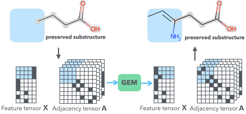
Figure 1: The proposed model, GEM, can generate a molecular graph by preserving its substructure(s), highlighted by gray, and complimenting the rests, highlighted by light blue.

To this end, we propose Graph Energy-based Model (GEM), an energy-based approach for molecular graph generation. GEM can generate molecules including specified substructures (see Figure 1). Energy-based models (EBMs [19]) are generative models that estimate a density of each data point by Boltzmann-Gibbs distribution with a scalar energy function $E$ as $p(\cdot)\propto\exp(-E(\cdot))$. Recently, several studies show that EBMs can generate high-quality images and audio as other deep generative models [9, 32, 2].

Inspired by these recent advances of EBMs in image and audio generation tasks, we propose an EBM approach for the molecular graph generation. Unlike the image and audio domains, the graph representation is discrete and constrained, where the techniques in the advances of EBMs are not applicable. To overcome this, GEM uses dequantization and gradient symmetrization. These modifications only slightly change the input graph representations, and off-the-shelf models can be used as generative models.

We empirically demonstrate that GEM can generate molecular graphs while preserving substructure constraints. Additionally, GEM can design molecules with desired properties, such as drug-likeliness, including specified substructures.

2 Background

2.1 De Novo Molecular Design

Novel compound generation using machine-learning requires a way of representing molecules by a data structure. String-based and graph-based are the two popular approaches for representing molecules. Many recent studies that apply deep neural networks for molecular design rely on an ASCII string format, Simplified Molecular-Input Line-Entry System (SMILES), which is popularly used in chemistry for describing molecules. In combination with SMILES based representations, various techniques were used, such as the variations of VAE [7, 18], RNN [29, 37], and GAN [10].

Another popular approach is to use graph-based representation, which seems to be more natural for describing molecules. Based on the advances in Graph Neural Networks [8], several graph-based approaches, such as GraphVAE [31], JT-VAE [14], and MolGAN [3], outperformed string-based methods in some of the metrics. Mol-CycleGAN [23] applied CycleGAN to the latent space of JT-VAE. Application of graph RNN (MolecularRNN by  [27]) and the flow model (GraphNVP by  [16]) also reported their advantages.

Apart from string and graph-based methods, there are other notable studies such as the following. [15] correctly handles the chemical constraints by hypergraph grammar and assures 100% validity. [39] defined molecule modification as a Markov decision process and achieved good scores in benchmarks by limiting the type of atoms. [38] applied grammatical evolution to the problem and succeeded in generating novel molecules. These approaches have different characteristics than string or graph-based methods and have future potential.

However, none of the previous studies have focused on a substructure preserving generation. Therefore, the effectiveness of compounds obtained from existing studies is too strongly dependent on the evaluation functions’ quality, e.g., penalized logP or QED (see section 4.1). In this paper, we propose to use another generative model, an energy-based model, to realize molecular generation while fixing specified substructures.

2.2 Energy-based Models

Energy-based models (EBMs, [19]) estimate probability densities using Boltzmann-Gibbs distributions as

$$p({\bm{z}})=\frac{\exp(-E({\bm{z}}))}{\int_{{\bm{z}}\in\mathcal{Z}}\exp(-E({\bm{z}}))\mathrm{d}{\bm{z}}},$$ (1)

where ${\bm{z}}$ is a datum in a certain open set $\mathcal{Z}$ in a finite-dimensional real space, and $E:\mathcal{Z}\rightarrow\mathbb{R}$ is a function called energy function. Though the RHS’s denominator is usually intractable, EBM methods allow sampling without explicitly obtaining it. High flexibility of the design of $E$ allows wide range of applications, including protein structure prediction [12, 5] and conformation prediction [22].

EBMs are also applied to high-resolution image generation, such as [9, 32, 4], and high-quality audio wave generation [2], which show comparable performance with other popular deep generative models, such as GANs and VAEs. Especially, [9] used a standard image classifier as the energy function, which inspires us to use an energy-based approach for graph generation. However, these image and audio data generations are on concrete domains, different from (molecular) graphs on discrete space.

Exceptionally, [24] applied EBMs to graphs by modeling the score function $\nabla_{\bm{z}}E$, i.e., using score matching [11], to generate adjacency matrices. In contrast, our approach, GEM, directly uses energy function $E$ and generates molecular graphs with multiple node and edge types.

3 Graph Energy-based Models

This section describes our proposed approach, Graph Energy-based Models, or GEM in short.

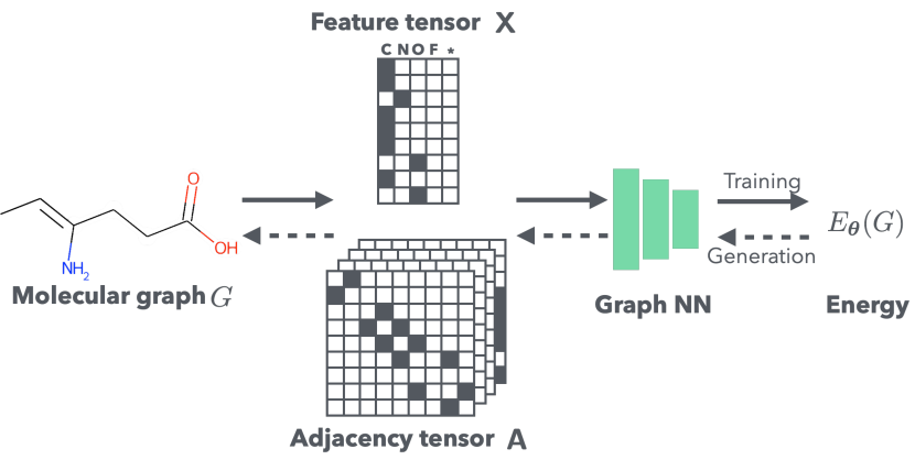
Figure 2: During training, GEM learns to assign lower energy to molecules in a dataset and higher energy to generated ones including invalid graphs. For property-targeted generation, molecules with desired properties are expected to have lower energy. GEM generates molecular graphs with lower energy using MCMC, which are expected to be valid molecules.

3.1 Notations

A molecular graph $G$ is an undirected graph depicted by a pair of tensors: a feature tensor ${\bm{\mathsfit{X}}}\in\{0,1\}^{N\times\#\mathcal{M}}$ and an adjacency tensor ${\bm{\mathsfit{A}}}\in\{0,1\}^{N\times N\times\#\mathcal{B}}$. The feature tensor ${\bm{\mathsfit{X}}}$ represents atoms in the molecule, and the adjacency tensor represents bonds among them. $N$ is the maximum number of atoms in molecules in a dataset, $\mathcal{M}$ is a set of considered atoms, e.g., $\mathcal{M}=\{\ce{C},\ce{N},\ce{O},\ce{F},\text{virtual node}\}$, and $\mathcal{B}$ is the set of bond types, i.e., $\mathcal{B}=\{\text{single},\text{double},\text{triple},\text{virtual bond}\}$. “virtual node” and “virtual bond” are used for padding in case the number of atoms in a given molecule is smaller than $N$.

For each triplet of $(N,\mathcal{M},\mathcal{B})$, there is a set of valid molecular graphs $\mathcal{G}=\mathcal{G}_{(N,\mathcal{M},\mathcal{B})}$. Validity includes the symmetry of adjacency tensor slices: ${\bm{\mathsfit{A}}}_{:,:,b}$ is a symmetric matrix for $b=1,2,\dots,\#\mathcal{B}$. Practically, we use datasets $\mathcal{D}\subset\mathcal{G}$.

3.2 Generating Graphs by EBMs

We propose to generate a novel molecule by using an energy function $E_{\bm{\theta}}:\mathcal{G}\to\mathbb{R}$, parameterized by a real vector ${\bm{\theta}}$. Specifically, we use a graph neural network to represent this parameterized function. The energy function is expected to assign smaller values to valid molecules and higher values to invalid ones. This energy function determines a Boltzmann-Gibbs distribution

$$p_{\bm{\theta}}(G)=\frac{\exp(-E_{\bm{\theta}}(G))}{\sum_{G^{\prime}\sim\mathcal{G}}\exp(-E_{\bm{\theta}}(G))},$$ (2)

from which molecules are expected to be sampled with a high probability. If graphs are continuous, we can sample graphs from this distribution by using stochastic gradient Langevin dynamics (SGLD, [35]):

$${\bm{\mathsfit{X}}}^{(t+1)} ={\bm{\mathsfit{X}}}^{(t)}+\frac{\alpha_{t}}{2}g_{\bm{\mathsfit{X}}}({\bm{\mathsfit{X}}}^{(t)},{\bm{\mathsfit{A}}}^{(t)})+\sqrt{\alpha_{t}}{\bm{\epsilon}}_{{\bm{\mathsfit{X}}}},$$ (3)

$${\bm{\mathsfit{A}}}^{(t+1)} ={\bm{\mathsfit{A}}}^{(t)}+\frac{\alpha_{t}}{2}g_{\bm{\mathsfit{A}}}({\bm{\mathsfit{X}}}^{(t)},{\bm{\mathsfit{A}}}^{(t)})+\sqrt{\alpha_{t}}{\bm{\epsilon}}_{{\bm{\mathsfit{A}}}},$$ (4)

where $\alpha_{t}\in\mathbb{R}^{+}$ is a step size, $g_{\bm{\mathsfit{X}}}=\nabla_{\bm{\mathsfit{X}}}E_{\bm{\theta}}$ and $g_{\bm{\mathsfit{A}}}=\nabla_{\bm{\mathsfit{A}}}E_{\bm{\theta}}$ are score functions, and ${\bm{\epsilon}}_{{\bm{\mathsfit{X}}}}$ and ${\bm{\epsilon}}_{{\bm{\mathsfit{A}}}}$ are standard normals. This generation (Equations 3 and 4) can also be achieved by directly estimating $g_{\bm{\mathsfit{X}}}$ and $g_{\bm{\mathsfit{A}}}$ as [24]. ${\bm{\mathsfit{X}}}^{(0)}$ and ${\bm{\mathsfit{A}}}^{(0)}$ are sampled from a uniform distribution on $[0,1]$. The distribution of $G^{(\infty)}=({\bm{\mathsfit{X}}}^{(\infty)},{\bm{\mathsfit{A}}}^{(\infty)})$ is asymptotically equal to $p_{\bm{\theta}}(G)$, and we assume that this property can be approximated with finite steps with a small constant state size, i.e., $\alpha_{t}=\alpha$, following the literature.

Actually, simply applying Equations 3 and 4 does not work in our case, because they do not consider the following requirements: 1. ${\bm{\mathsfit{X}}}$and ${\bm{\mathsfit{A}}}$ are discrete, and 2. slices of ${\bm{\mathsfit{A}}}$ is symmetric. To fix the first issue, we relax the domains of ${\bm{\mathsfit{X}}}$ and ${\bm{\mathsfit{A}}}$ to be $(0,1)^{N\times\#\mathcal{M}}$ and $(0,1)^{N\times N\times\#\mathcal{B}}$. For discrete tensors from datasets, we modify them by using dequantization and applying softmax function along the last axes. Dequantization is a technique used in [16], which adds random values to the tensor elements:

$${\bm{\mathsfit{X}}}\leftarrow{\bm{\mathsfit{X}}}+c{\bm{\mathsfit{U}}}_{{\bm{\mathsfit{X}}}},~{}~{}{\bm{\mathsfit{A}}}\leftarrow{\bm{\mathsfit{A}}}+c{\bm{\mathsfit{U}}}_{{\bm{\mathsfit{A}}}},$$ (5)

where $c\in(0,1)$ is a scaling parameter, and ${\bm{\mathsfit{U}}}_{{\bm{\mathsfit{X}}}},{\bm{\mathsfit{U}}}_{{\bm{\mathsfit{A}}}}$ are uniform noise on $(0,1)$. We set $c=0.9$ in the experiments.

To avoid sampled adjacency tensors being asymmetric, we sample ${\bm{\mathsfit{A}}}^{(0)}$ and ${\bm{\epsilon}}_{\bm{\mathsfit{A}}}$ from symmetric distributions, where

$$({\bm{\mathsfit{A}}}^{(0)})_{i,j,b}=({\bm{\mathsfit{A}}}^{(0)})_{j,i,b},~{}~{}({\bm{\epsilon}}_{{\bm{\mathsfit{A}}}})_{i,j,b}=({\bm{\epsilon}}_{{\bm{\mathsfit{A}}}})_{j,i,b},$$

for $i,j\in\{1,2,\dots,N\}$ and $b\in\{1,2\dots,\#\mathcal{B}\}$. Additionally, the score function $g_{\bm{\mathsfit{A}}}$ needs to be symmetric, which we will describe in the next section.

3.3 Symmetrize Gradient of Adjacency Tensor

We use a neural network based on Relational GCN (RGCN) [28] as an energy function. RGCN is a graph convolutional neural network for graphs with multiple edge types. For each graph $G=({\bm{\mathsfit{X}}},{\bm{\mathsfit{A}}})$, the $l$th RGCN layer processes node representation ${\bm{\mathsfit{H}}}_{l}\in\mathbb{R}^{N\times C}$ as

$${\bm{\mathsfit{H}}}_{l+1}=\sigma\left({\bm{\mathsfit{H}}}_{l}W_{l}^{(0)}+\sum_{b=1}^{\#\mathcal{B}}{\bm{\mathsfit{A}}}_{:,:,b}{\bm{\mathsfit{H}}}_{l}W_{l}^{(b)}\right),$$ (6)

where ${\bm{\mathsfit{H}}}_{0}={\bm{\mathsfit{X}}}$, $W_{l}^{(0)},W_{l}^{(b)}\in\mathbb{R}^{C\times D}$ are learnable parameters, $\sigma$ is a nonlinear activation function, and $C,D$ are input and output feature dimensions. After several RGCN layers, a graph-level representation is obtained by the aggregation of [20]. This representation is transformed into a scalar value $E_{\bm{\theta}}(G)$ by a multi layer perceptron.

Crucially, with this energy function, the score function $g_{\bm{\mathsfit{A}}}$ is asymmetric. Indeed, by focusing on the first layer of RGCN layers and ignoring the nonlinear activation for simplicity, we obtain a Jacobian tensor of

$$\frac{\partial{\bm{\mathsfit{H}}}_{1}}{\partial({\bm{\mathsfit{A}}})_{i,j,b}}=\frac{\partial{\bm{\mathsfit{A}}}_{:,:,b}{\bm{\mathsfit{X}}}W_{b}^{(1)}}{\partial({\bm{\mathsfit{A}}})_{i,j,b}}={\bm{J}}^{(i,j)}{\bm{\mathsfit{X}}}W_{b}^{(1)},$$ (7)

where ${\bm{J}}^{(i,j)}$ denotes a single entry matrix of $1$ at $(i,j)$ and $0$ elsewhere [26]. This gradient is not symmetric for each $b$. To remedy this, we modify Equation 6 as

$${\bm{\mathsfit{H}}}_{l+1}=\sigma\left({\bm{\mathsfit{H}}}_{l}W_{l}^{(0)}+\sum_{b=1}^{\#\mathcal{B}}\frac{1}{2}({\bm{\mathsfit{A}}}_{:,:,b}+{\bm{\mathsfit{A}}}_{:,:,b}^{\top}){\bm{\mathsfit{H}}}_{l}W_{l}^{(b)}\right).$$ (8)

Though this modification does not change the output because each ${\bm{\mathsfit{A}}}_{:,:,b}$ is symmetric by definition, now the Jacobian tensor is also symmetrized as

$$\frac{\partial{\bm{\mathsfit{H}}}_{1}}{\partial({\bm{\mathsfit{A}}})_{i,j,b}}=\frac{1}{2}(J^{(i,j)}+J^{(j,i)}){\bm{\mathsfit{X}}}W_{b}^{(1)},$$ (9)

from which we can deduce $\displaystyle\frac{\partial E_{\bm{\theta}}}{\partial({\bm{\mathsfit{A}}})_{i,j,b}}=\frac{\partial E_{\bm{\theta}}}{\partial({\bm{\mathsfit{A}}})_{j,i,b}}$, the symmetry of the score function $g_{\bm{\mathsfit{A}}}$. Practically, the modification of Equation 8 can be separately done before the forward pass of the model, which means the actual modification to the off-the-shelf models is minimum. In the experiments, we use the abovementioned RGCN variant, which is also used in other graph-based molecular generation methods [3, 16].

3.4 Training of GEM

GEM is trained to maximize likelihood of $p_{\bm{\theta}}$ defined in Equation 2. Equivalently, this objective minimizes the Kullback-Leibler divergence between data and model distribution $D_{\mathrm{KL}}(p_{\mathcal{D}}||p_{\bm{\theta}})$. To optimize the energy function $E_{\bm{\theta}}$, we can use stochastic gradient of

$$\nabla_{\bm{\theta}}\mathbb{E}_{\mathcal{D}}\left[\log p_{\bm{\theta}}(G)\right]=\mathbb{E}_{\mathcal{D}}\left[\nabla_{\bm{\theta}}E_{\bm{\theta}}(G)\right]-\mathbb{E}_{p_{\bm{\theta}}(G^{\prime})}\left[\nabla_{\bm{\theta}}E_{\bm{\theta}}(G^{\prime})\right].$$ (10)

At the LHS’s second term, samples from the model $G^{\prime}\sim p_{\bm{\theta}}(G^{\prime})$ are used. As discussed in Section 3.2, we use a finite step of SGLD to approximate this sampling, resulting in diverged samples from the model distribution. To remedy this problem, we use the persistent contrastive divergence (PCD, [33]), which reuses the past generated samples.

We summarize the training procedure in Algorithm 1. Additionally, we found that penalizing $\{E_{\bm{\theta}}(G)\}^{2}$ improves empirical performance.

Algorithm 1 Training of GEM

Energy function: $E_{\bm{\theta}}$

Reinitialization probability: $\rho$

while not converge :

     Sample $G=({\bm{\mathsfit{X}}}_{G},{\bm{\mathsfit{A}}}_{G})$ from dataset $\mathcal{D}$

     Sample $({\bm{\mathsfit{X}}}_{B},{\bm{\mathsfit{A}}}_{B})$ from PCD buffer $B$ with probability $1-\rho$, otherwise sample $({\bm{\mathsfit{X}}}_{B},{\bm{\mathsfit{A}}}_{B})$ from uniform distribution on $(0,1)$

     SGLD steps in Equations 3 and 4:$({\bm{\mathsfit{X}}}_{B},{\bm{\mathsfit{A}}}_{B})\mapsto({\bm{\mathsfit{X}}}^{\prime}_{B},{\bm{\mathsfit{A}}}^{\prime}_{B})$

     Compute energy loss$\ell_{\bm{\theta}}=\nabla_{\bm{\theta}}E_{\bm{\theta}}({\bm{\mathsfit{X}}}_{G},{\bm{\mathsfit{A}}}_{G})-\nabla_{\bm{\theta}}E_{\bm{\theta}}({\bm{\mathsfit{X}}}^{\prime}_{B},{\bm{\mathsfit{A}}}^{\prime}_{B})$

     For property-targeted generation, add regression loss

$\ell_{\bm{\theta}}\leftarrow\ell_{\bm{\theta}}+\lvert E_{{\bm{\theta}}}(G)-y_{G}\rvert^{2}$, where $y_{G}$ is a property value of $G$

     Add $({\bm{\mathsfit{X}}}^{\prime}_{B},{\bm{\mathsfit{A}}}^{\prime}_{B})$ to $B$

     Update ${\bm{\theta}}$ with stochastic gradient $\nabla_{\bm{\theta}}\ell_{\bm{\theta}}$

3.5 Generation by GEM

Once the energy function $E_{\bm{\theta}}$ is trained, GEM can generate molecular graphs using SGLD in Equations 3 and 4 unconditionally. Additionally, GEM can design molecules while preserving substructures and optimizing desired properties.

Substructure Preserving Generation

The most characteristic ability of GEM is to generate molecular graphs while fixing specified substructures. Because GEM samples molecular graphs in the input space by SGLD, this ability is achieved by updating parts of graph representation (see also Figures 1 and 3).

To fix substructures, we apply masks to both feature and adjacency tensors. Suppose the number of atoms in a given substructure is $S<N$, where $N$ is the maximum number of atoms in molecules of a dataset. Because GEM is permutation invariant to an input representation, we can re-index atoms in the substructure to $1,2,\dots,S$ such that the $S$th atom to be connected with the rest part, without loss of generality. Then, we use a mask to update only a part of the feature tensor corresponding to $S+1,S+2,\dots,N$th atoms and fix the atoms in the substructure. Similarly, we only update connections among $S,S+1,\dots,N$th atoms and fix the connections among the rests by masking the adjacency tensor. This masking can be extended to appending the rest parts to multiple atoms.

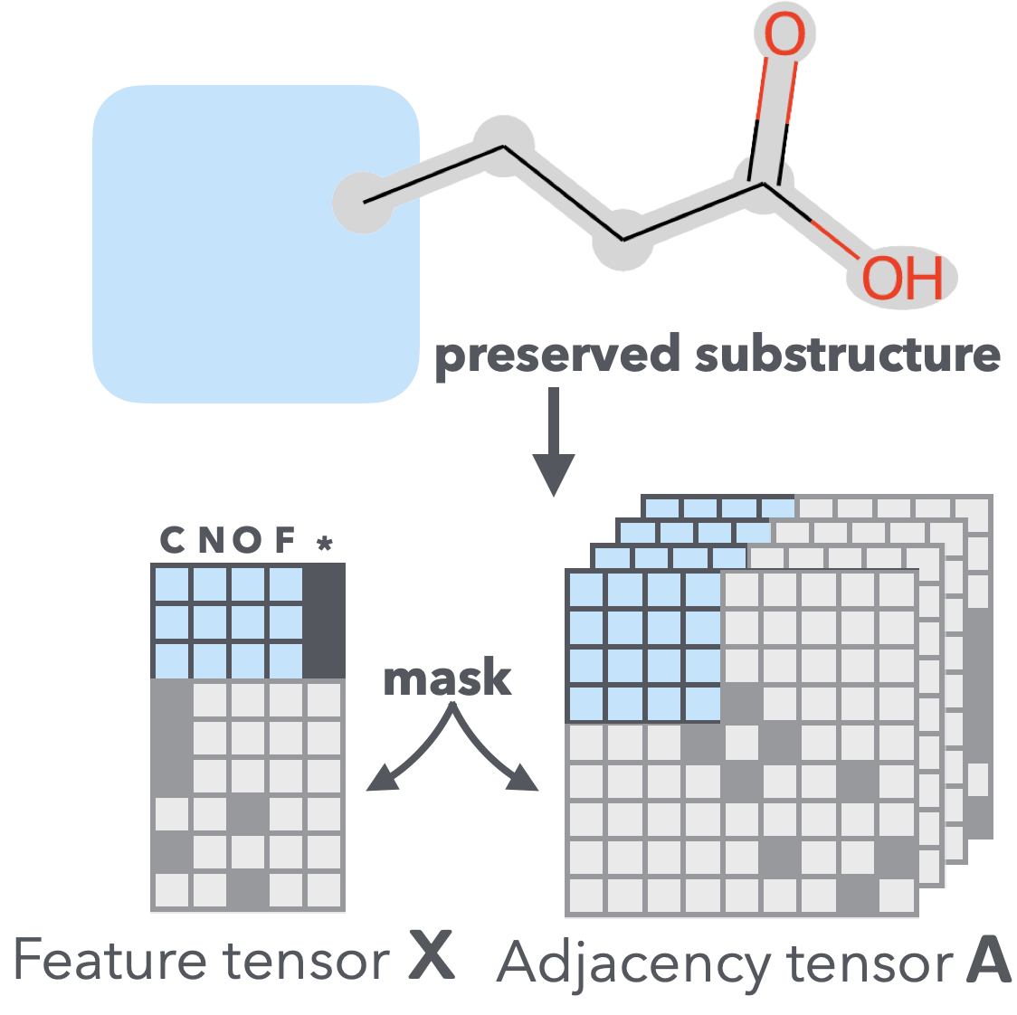
Figure 3: GEM enables substructure preserving generation by masking feature and adjacency tensors (masked by light gray) and updating the rests parts (highlighted by light blue).

Property-targeted Generation

GEM explicitly estimates energy function $E_{\bm{\theta}}$. One of the most appealing benefits of this modeling is property-targeted molecular generation, by regarding an objective property as energy. Specifically, lower energy is assigned to molecules with desired properties, and vice versa. Because GEM samples molecular graphs with lower energy, this assignment brings GEM to generate compounds with desired properties. For this purpose, GEM is trained jointly with a regression loss $\mathbb{E}_{G\sim\mathcal{D}}\lvert E_{{\bm{\theta}}}(G)-y_{G}\rvert^{2}$, where $y_{G}$ is a property, such as drug-likeliness, of a molecule $G$.

4 Experiments

4.1 Experimental Settings

Datasets

We used QM9 [36] and ZINC-250k [13] as datasets $\mathcal{D}$. QM9 and ZINC-250k contain $1.3\times 10^{5}$ and $2.5\times 10^{5}$ molecules, respectively. Following the preprocessing protocols in [16], we kekulize each molecule in each dataset and ignore hydrogens as the SMILES format. As a result, the maximum number of atoms in a molecule $N$ is $9$ for QM9 9 and $38$ for ZINC-250k. The number of atom types $\#\mathcal{M}$ including the virtual node is $5$ for QM9 and $10$ for ZINC-250k. The number of bond types $\#\mathcal{B}$ is 4, namely $\mathcal{B}=\{\text{single},\text{double},\text{triple},\text{virtual bond}\}$, for both datasets. We also followed the data split of [16].

Implementation Details

We used PyTorch v1.7 [25] for model implementation, chainer-chemistry v0.7 for data preprocessing, and RDKit v2020.09 for handling molecule information.

Each input feature tensor is embedded in 16-dimensional space and processed by a two-layer RGCN of 128 hidden dimensions. Its output is aggregated in a 256-dimensional space and converted to scalar energy by an MLP of $(1024,512)$ hidden units. The hyperbolic tangent function is used as an activation function, and the sigmoid function $\varsigma(x)=\{1+\exp(-x)\}^{-1}$ is applied to the final output that restricts the range to $[0,1]$.

We trained GEM using Adam [17] with a learning rate of $1.0\times 10^{-4}$ for $30$ epochs. For SGLD, we set a step size $\alpha$ to $1.0\times 10^{-4}$ and the number of steps to $40$. Following [9, 4], we set the buffer size of PCD to $10^{4}$ and the reinitialization probability $\rho$ (see Algorithm 1) to $5.0\times 10^{-2}$, and reduced the effect of additive noise by multiplying $0.1$ to the standard deviation as common practice. For SGLD, we used an exponential moving average of the model with a decay rate of $1.0\times 10^{-3}$ for the stability.

To generate molecular graphs, we used SGLD of step size of $1.0\times 10^{-1}$ for QM9 and $1.0\times 10^{-2}$ for ZINC-250k, and the number of steps of $10^{3}$. Adding noise in Equations 3 and 4 sometimes turns once generated valid molecular graphs into invalid ones. Therefore, we record all valid graphs generated at each step. We discarded the graphs generated during the first 100 steps to reduce the effects of initial states.

Objective Properties

For property-targeted generation, we use the following commonly used properties:

Penalized logP (solubility):

hydrophobicity, namely the logarithm of octanol-water partition coefficient penalized by synthetic accessibility and ring penalty, and

Drug-likeliness (QED):

measure of drug likeliness, specifically the quantitative estimate of drug-likeness [1].

We used RDKit to compute these properties of each compound. In the experiments, we normalize these measures for each molecule into $[0,1]$ as $0$ to be a favorable property value because GEM generates molecular graphs with lower energy.

4.2 Substructure Preserving Generation

Figure 4 shows examples of substructure preserving generation using GEM, which is impossible for existing graph-based generative methods. As conditioning substructures, we used propane CCC, acetone CC(=O)C, and butanoic acid CCCC(=O)O. Carbon atoms at the edge of each molecule is specified to append generated parts. GEM can successfully generate molecules while preserving specified substructures.

Substructure preserving generation can be combined with property-targeted optimization. Figure 5 presents generated molecules by GEM trained on QM9 and ZINC-250k with conditioning substructure of benzene c1ccccc1. GEM is trained on each dataset with regression loss to drug-likeliness as presented in Algorithm 1. As can be seen, GEM generates molecules with improved QED values (up to $0.19$), while preserving the benzene substructure.

As more complex examples, Figures 6 and 7 show generated molecular graphs conditioned by piperazine C1CNCCN1 and 4-Chlorodiphenylmethane c1ccc(cc1)Cc2ccc(cc2)Cl, which are used in [30] as starting materials of retro-synthesis. GEM is trained on ZINC-250k jointly with regression loss to drug-likeliness. For piperazine C1CNCCN1 (Figure 6), we specified both of two nitrogen atoms to append generated parts. Such generation with complex conditioning is almost impossible for SMILE-based methods that may only append generated parts subsequent to given substructures. Contrarily, GEM enjoys high flexibility of substructure-preserving generation.

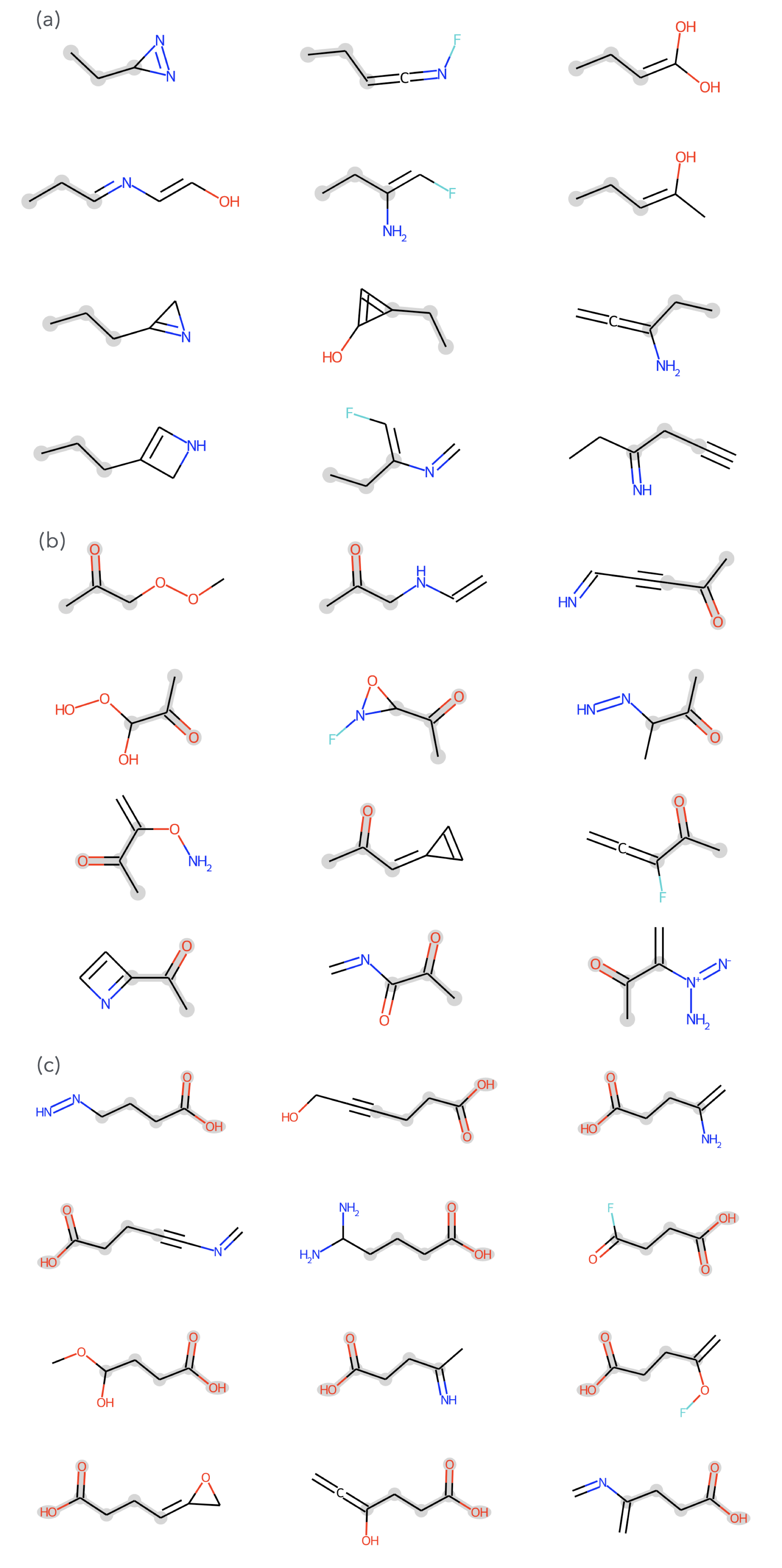
Figure 4: Randomly selected molecules of substructure preserving generation. Conditioned substructures are (a) propane CCC, (b) acetone CC(=O)C, and (c) butanoic acid CCCC(=O)O, which are highlighted by light gray.

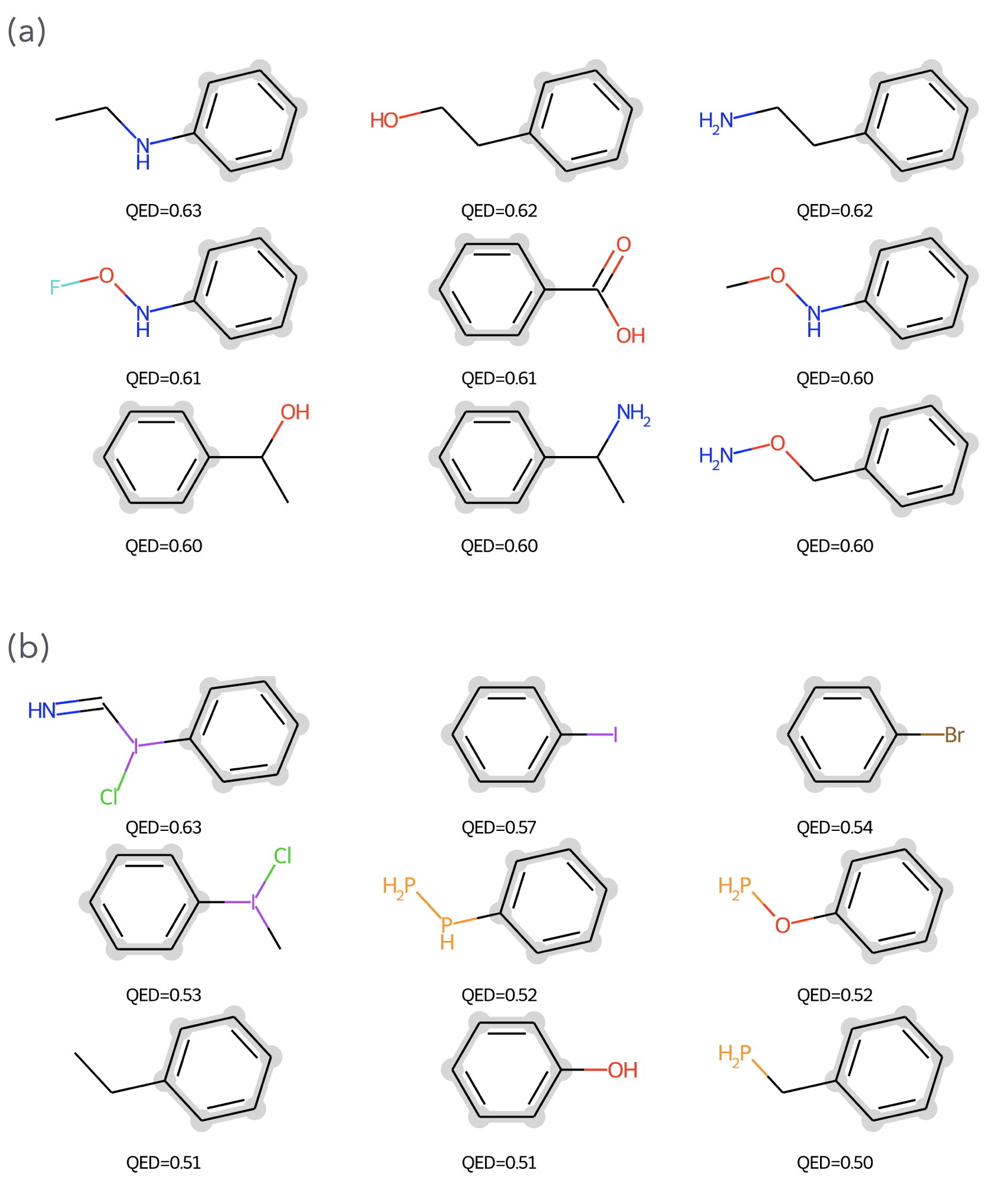
Figure 5: Generated molecules while preserving a substructure, benzene c1ccccc1, and optimizing drug-likeliness (QED). GEM is trained on QM9 for (a) and ZINC-250k for (b). The preserved substructure is highlighted by light gray. Generated molecules with the best QED score are presented. The QED value of the original substructure is $0.44$.

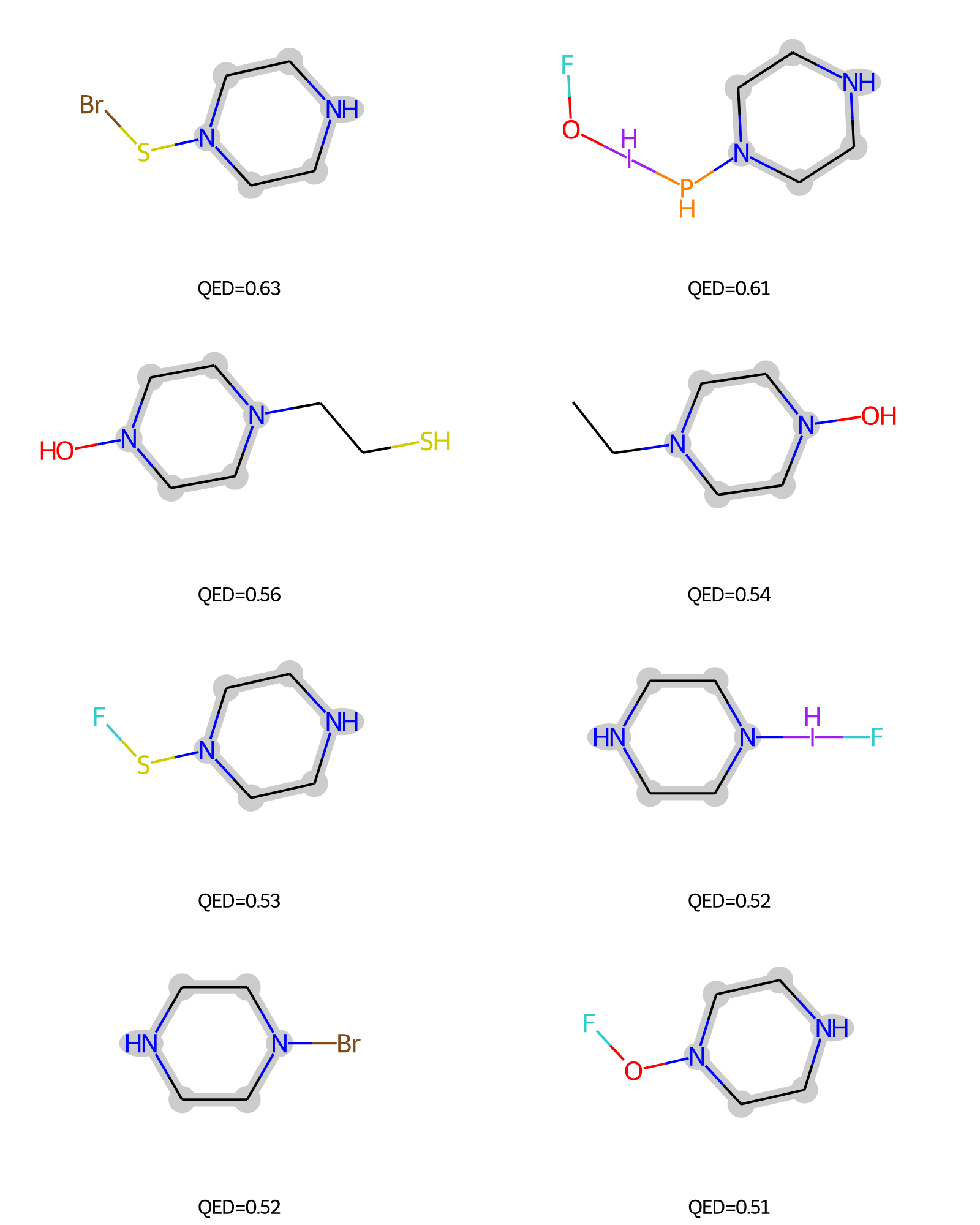
Figure 6: Generated molecules while preserving a substructure, piperazine C1CNCCN1, and optimizing drug likeliness (QED). GEM is trained on ZINC-250k. The preserved substructure is highlighted by light gray. Generated molecules with the best QED scores are presented. QED of the original substructure is $0.40$.

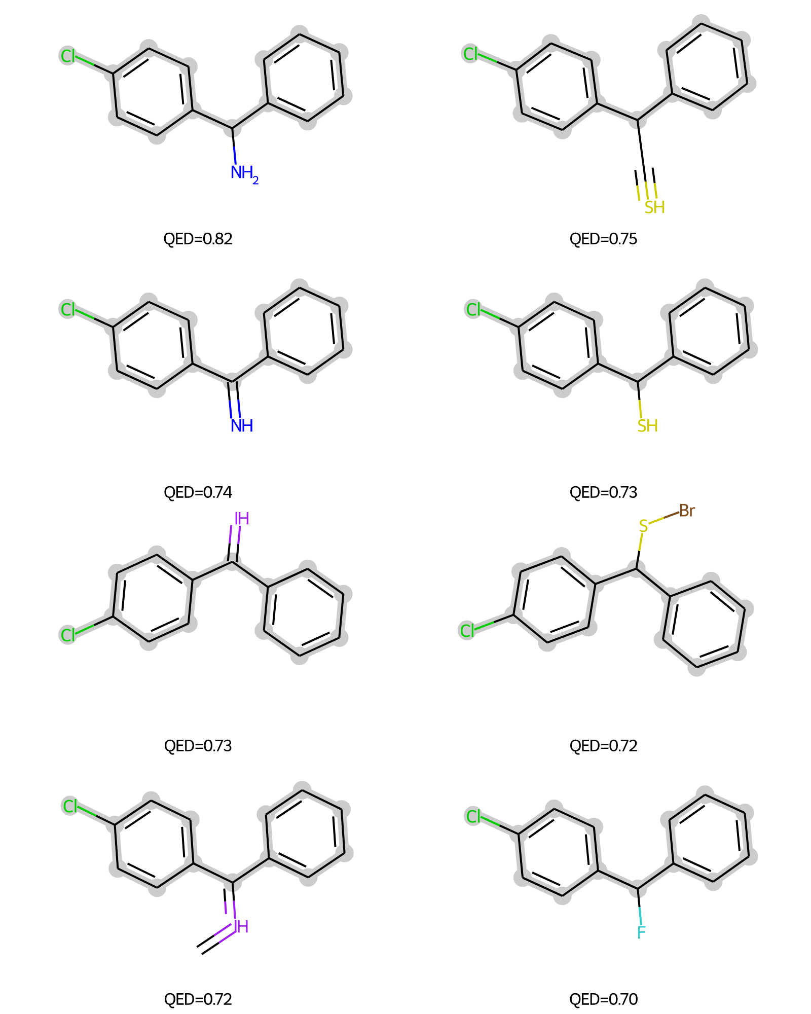
Figure 7: Generated molecules while preserving a substructure, c1ccc(cc1)Cc2ccc(cc2)Cl, and optimizing drug likeliness (QED). GEM is trained on ZINC-250k. The preserved substructure is highlighted by light gray. Generated molecules with the best QED scores are presented. QED of the original substructure is $0.69$.

5 Discussion

5.1 Improving Given Molecules

So far, GEM creates compounds from uniform noise of the initial states of generation (Equations 3 and 4) with fixed substructures. Additionally, GEM can improve given molecules with respect to targeted properties by substituting them for random initial states and removing masks for preservation. We sampled $10^{3}$ molecules from the validation set of QM9 and optimized penalized logP using GEM. Figure 8 compares penalized logP of molecules generated by GEM trained on QM9 with regression loss to penalized logP and the original molecules from the dataset. GEM can effectively optimize penalized logP from the original data. Notice that this property improvement can further be integrated into substructure preserving generation.

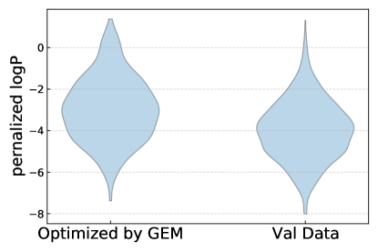
Figure 8: Penalized logP comparison of molecular graphs optimized by GEM from validation data and the original molecules.

5.2 Comparison with Random Generation

We found SGLD (Equations 3 and 4) ignoring score functions and only adding noise, namely, ${\bm{\mathsfit{X}}}^{(t+1)}={\bm{\mathsfit{X}}}^{(t)}+\sqrt{\alpha}{\bm{\epsilon}}_{{\bm{\mathsfit{X}}}},{\bm{\mathsfit{A}}}^{(t+1)}={\bm{\mathsfit{A}}}^{(t)}+\sqrt{\alpha}{\bm{\epsilon}}_{{\bm{\mathsfit{A}}}}$, can sometimes produce valid molecular graphs. In Figure 9, we compare penalized logP of molecular graphs generated by GEM and noise using the substructure condition of acetone. In this setting, GEM is trained on QM9 jointly to maximize penalized logP. As can be observed, GEM can generate molecular graphs with desired property, penalized logP. These results indicate that generated graphs are sampled from the graph distribution induced from the trained energy function. Additionally, SGLD without noise, i.e., ${\bm{\mathsfit{X}}}^{(t+1)}={\bm{\mathsfit{X}}}^{(t)}+\frac{\alpha}{2}g_{\bm{\mathsfit{X}}}({\bm{\mathsfit{X}}}^{(t)},{\bm{\mathsfit{A}}}^{(t)}),{\bm{\mathsfit{A}}}^{(t+1)}={\bm{\mathsfit{A}}}^{(t)}+\frac{\alpha}{2}g_{\bm{\mathsfit{A}}}({\bm{\mathsfit{X}}}^{(t)},{\bm{\mathsfit{A}}}^{(t)})$ failed to produce graphs, which shows the importance of both score functions and noise in GEM.

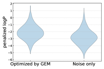
Figure 9: Penalized logP comparison of molecular graphs generated by GEM and noise using a substructure of acetone.

5.3 Comparison with Non Substructure-preserving Methods

We observed that GEM produces less valid graphs when substructures are not specified. As a reference, we compare GEM with other graph-based molecular generation methods. Table 1 presents scores of validity and novelty of GEM and other approaches, namely GraphNVP [16], MolGAN [3], and RVAE [21], which use the normalizing flow, GAN, and VAE as backend generative methods, respectively. These models generate adjacency tensors in a one-shot manner. For comparison, we generate molecular graphs from 1,000 different random pairs of feature and adjacency tensors. Unlike baseline methods, the metrics of GEM are computed using unique molecules, which disallows duplication. This design may underestimate the ability of GEM.

Table 1: The results of non substructure-preserving molecular graph generation. All models are trained on QM9. Baseline results are borrowed from the original papers. For GEM, average and standard deviation of five runs are reported.

Method	Validity $(\uparrow)$	Novelty $(\uparrow)$
GEM	0$7.1\pm 0.6$	$92.4\pm 2.9$
GEM (CC(=O)C)	$49.2\pm 2.4$	$89.0\pm 0.7$
GEM (CCCC(=O)O)	$22.9\pm 0.9$	$100\pm 0.0$
GraphNVP	$83.1\pm 0.5$	$58.2\pm 1.9$
MolGAN	98.1	94.2
RVAE	96.6	97.5

5.4 Future Direction

Table 1 shows limited validity of generated molecules by GEM especially when substructures are not given. Furthermore, we observed that GEM fails to generate molecular graphs from scratch, when the model is trained on ZINC-250k. We believe that this failure is due to the scarcity of valid graphs in large search space: for ZINC-250k, shapes of input tensors are $38\times 10$ for feature tensors and $38\times 38\times 4$ for adjacency tensors.

One possible approach to overcome this limitation is to use lower dimensional continuous latent spaces as other generative approaches, such as [31, 14, 21, 3]. Such latent spaces may enable more efficient search and higher validity, but, at the same time, hinder flexible substructure-preserving generation. Alternatively, GEM has room for introducing chemical rules to restrict its search space, such as inferring bond types of adjacency tensors from atom types of feature tensors. GEM uses the minimum prior knowledge for molecular graph generation, and thus, is potentially applicable for more general graph generation with subgraph preservation. We leave these possible improvements for future work.

6 Conclusion

In this paper, we have proposed GEM, an energy-based generative model for molecular graphs that can exactly preserve specified substructures, which is nearly impossible for existing approaches. GEM can design novel molecules with optimized properties, because energy function is explicitly instantiated. We have empirically demonstrate these abilities. Also importantly, GEM can be extended to general graph generation methods that can fix subgraphs.

By specifying available compounds as fixed substructures, GEM can design novel molecules that are expected to be easier to synthesize not only in silico but also in vitro. We hope GEM opens a new direction of de novo design.

References

- [1] G. Bickerton, Gaia V. Paolini, Jérémy Besnard, Sorel Muresan and Andrew L. Hopkins In Nature Chemistry 4, 2012, pp. 90–98
- [2] Nanxin Chen, Yu Zhang, Heiga Zen, Ron J. Weiss, Mohammad Norouzi and William Chan “WaveGrad: Estimating Gradients for Waveform Generation” In ICLR, 2020
- [3] Nicola De Cao and Thomas Kipf “MolGAN: An implicit generative model for small molecular graphs” In ICML 2018 workshop on Theoretical Foundations and Applications of Deep Generative Models, 2018
- [4] Yilun Du, Shuang Li, Joshua Tenenbaum and Igor Mordatch “Improved Contrastive Divergence Training of Energy Based Models” In arXiv:2012.01316, 2020
- [5] Yilun Du, Joshua Meier, Jerry Ma, Rob Fergus and Alexander Rives “Energy-based models for atomic-resolution protein conformations” In ICLR, 2020
- [6] Wenhao Gao and Connor W. Coley “The Synthesizability of Molecules Proposed by Generative Models” In Journal of Chemical Information and Modeling 60.12, 2020, pp. 5714–5723
- [7] R. Gómez-Bombarelli, J.. Wei, D. Duvenaud, J.. Hernández-Lobato, B. Sánchez-Lengeling, D. Sheberla, J. Aguilera-Iparraguirre, T.. Hirzel, R. Adams and A. Aspuru-Guzik “Automatic chemical design using a data-driven continuous representation of molecules” In ACS central science 4.2 ACS Publications, 2018, pp. 268–276
- [8] M. Gori, G. Monfardini and F. Scarselli “A new model for learning in graph domains” In IJCNN, 2005
- [9] Will Grathwohl, Kuan-Chieh Wang, Joern-Henrik Jacobsen, David Duvenaud, Mohammad Norouzi and Kevin Swersky “Your classifier is secretly an energy based model and you should treat it like one” In ICLR, 2020
- [10] Gabriel Lima Guimaraes, Benjamin Sanchez-Lengeling, Carlos Outeiral, Pedro Luis Cunha Farias and Alán Aspuru-Guzik “Objective-Reinforced Generative Adversarial Networks (ORGAN) for Sequence Generation Models” In arXiv:1705.10843, 2018
- [11] Aapo Hyvärinen “Estimation of Non-Normalized Statistical Models by Score Matching” In JMLR 6.24, 2005, pp. 695–709 URL: http://jmlr.org/papers/v6/hyvarinen05a.html
- [12] John Ingraham, Adam Riesselman, Chris Sander and Debora Marks “Learning Protein Structure with a Differentiable Simulator” In ICLR, 2019
- [13] John J Irwin and Brian K Shoichet “ZINC – A free database of commercially available compounds for virtual screening” In Journal of Chemical Information and Modeling 45, 2015
- [14] Wengong Jin, Regina Barzilay and Tommi Jaakkola “Junction Tree Variational Autoencoder for Molecular Graph Generation” In ICML, 2018
- [15] Hiroshi Kajino “Molecular Hypergraph Grammar with Its Application to Molecular Optimization” In ICML, 2019
- [16] Madhawa Kaushalya, Ishiguro Katushiko, Nakago Kosuke and Abe Motoki “GraphNVP: An Invertible Flow Model for Generating Molecular Graphs” In NeurIPS, 2019
- [17] Diederik P. Kingma and Jimmy Ba “Adam: A Method for Stochastic Optimization” In ICLR, 2015
- [18] M.. Kusner, B. Paige and J.. Hernández-Lobato “Grammar variational autoencoder” In ICML, 2017
- [19] Yann LeCun, Sumit Chopra, Raia Hadsell, M Ranzato and F Huang “A tutorial on energy-based learning” In Predicting Structured Data 1.0, 2006
- [20] Yujia Li, Daniel Tarlow, Marc Brockschmidt and Richard Zemel “Gated Graph Sequence Neural Networks” In ICLR, 2016
- [21] Tengfei Ma, Jie Chen and Cao Xiao “Constrained Generation of Semantically Valid Graphs via Regularizing Variational Autoencoders” In NeurIPS, 2018
- [22] Elman Mansimov, Omar Mahmood, Seokho Kang and Kyunghyun Cho “Molecular Geometry Prediction using a Deep Generative Graph Neural Network” In Scientific Report 9, 2019
- [23] Łukasz Maziarka, Agnieszka Pocha, Jan Kaczmarczyk, Krzysztof Rataj, Tomasz Danel and Michał Warchoł “Mol-CycleGAN: a generative model for molecular optimization” In Journal of Cheminformatics 12.2, 2020
- [24] Chenhao Niu, Yang Song, Jiaming Song, Shengjia Zhao, Aditya Grover and Stefano Ermon “Permutation Invariant Graph Generation via Score-Based Generative Modeling” In AISTATS, 2020
- [25] Adam Paszke et al. “PyTorch: An Imperative Style, High-Performance Deep Learning Library” In NeurIPS, 2019
- [26] Kaare Petersen and Michael Pedersen “The Matrix Cookbook”, 2006
- [27] Mariya Popova, Mykhailo Shvets, Junier Oliva and Olexandr Isayev “MolecularRNN: Generating realistic molecular graphs with optimized properties” In arXiv:1905.13372, 2019
- [28] Michael Schlichtkrull, Thomas N. Kipf, Peter Bloem, Rianne Berg, Ivan Titov and Max Welling “Modeling Relational Data with Graph Convolutional Networks” In European Semantic Web Conference, 2018
- [29] Marwin H.. Segler, Thierry Kogej, Christian Tyrchan and Mark P. Waller “Generating Focused Molecule Libraries for Drug Discovery with Recurrent Neural Networks” In ACS Central Science 4.1, 2018, pp. 120–131
- [30] Ryosuke Shibukawa, Shoichi Ishida, Kazuki Yoshizoe, Kunihiro Wasa, Kiyosei Takasu, Yasushi Okuno, Kei Terayama and Koji Tsuda “CompRet: a comprehensive recommendation framework for chemical synthesis planning with algorithmic enumeration” In Journal of Cheminformatics 12.52, 2020
- [31] Martin Simonovsky and Nikos Komodakis “GraphVAE: Towards Generation of Small Graphs Using Variational Autoencoders” In arXiv:1802.03480, 2018
- [32] Yang Song and Stefano Ermon “Improved Techniques for Training Score-Based Generative Models” In NeurIPS, 2020
- [33] Tijmen Tieleman “Training Restricted Boltzmann Machines Using Approximations to the Likelihood Gradient” In ICML, 2008
- [34] D. Weininger “SMILES, a chemical language and information system. 1. Introduction to methodology and encoding rules” In Journal of chemical information and computer sciences 28.1 ACS Publications, 1988, pp. 31–36
- [35] Max Welling and Yee Whye Teh “Bayesian Learning via Stochastic Gradient Langevin Dynamics” In ICML, 2011
- [36] Zhenqin Wu, Bharath Ramsundar, Evan N. Feinberg, Joseph Gomes, Caleb Geniesse, Aneesh S. Pappu, Karl Leswing and Vijay Pande “MoleculeNet: a benchmark for molecular machine learning” In Chemical Science 9, 2018, pp. 513–530
- [37] X. Yang, J. Zhang, K. Yoshizoe, K. Terayama and K. Tsuda “ChemTS: an efficient python library for de novo molecular generation” In Science and technology of advanced materials 18.1, 2017, pp. 972–976
- [38] Naruki Yoshikawa, Kei Terayama, Masato Sumita, Teruki Homma, Kenta Oono and Koji Tsuda “Population-based De Novo Molecule Generation, Using Grammatical Evolution” In Chemistry Letters 47.11, 2018, pp. 1431–1434
- [39] Zhenpeng Zhou, Steven Kearnes, Li Li, Richard N. Zare and Patrick Riley “Optimization of Molecules via Deep Reinforcement Learning” In Scientific Reports 9.1, 2019, pp. 10752