Liquidation, Leverage and Optimal Margin in Bitcoin Futures Markets

Abstract

Using the generalized extreme value theory to characterize tail distributions, we address liquidation, leverage, and optimal margins for bitcoin long and short futures positions. The empirical analysis of perpetual bitcoin futures on BitMEX shows that (1) daily forced liquidations to outstanding futures are substantial at 3.51%, and 1.89% for long and short; (2) investors got forced liquidation do trade aggressively with average leverage of 60X; and (3) exchanges should elevate current 1% margin requirement to 33% (3X leverage) for long and 20% (5X leverage) for short to reduce the daily margin call probability to 1%. Our results further suggest normality assumption on return significantly underestimates optimal margins. Policy implications are also discussed.

Key words: Bitcoin futures; Liquidation; Margin; Leverage; Generalized extreme value theory

JEL Classification: G11, G13, G32

1 Introduction

The largest cryptocurrency, bitcoin, accounts for more than 70% of the total market capitalization reported by CoinMarketCap on 14 December 2020. Compared with other traditional assets, bitcoin price is more volatile: 30-day volatility reaches to 167.24% on 31 March, 2020. This extraordinarily high price volatility imposes a tremendous risk to various market participants, see Chaim and Laurini, (2018), Alexander et al., 2020b , Deng et al., (2020) and Scaillet et al., (2020).

Futures contracts are commonly used to hedge spot price risk. We refer this rich field to Figlewski, (1984), Daskalaki and Skiadopoulos, (2016) and Alexander et al., (2019) for traditional equity, commodity and currency markets. For bitcoin futures markets, the hedge effectiveness and improvement of portfolio performance are well studied in Alexander et al., 2020a , Sebastião and Godinho, (2020), Deng et al., (2019) and others. By November 2020, bitcoin futures monthly trading volume reached to $1.32 trillion notional, reported by CryptoCompare.

In this paper, our leitmotif to study optimal margins stems from several facts observed in bitcoin futures markets. First, as is well-known, the margin requirement is one of the key market designs by exchanges to maintain the integrity, liquidity, and efficiency of futures markets, see Figlewski, (1984). However, to the best of our knowledge, existing researches on bitcoin futures’ margin are limited. One exception is the recent work of Alexander et al., 2020b that investigates the optimal bitcoin futures hedge under investors’ margin constraints and default aversion. Second, bitcoin futures contracts are traded across several exchanges, from regulated exchanges such as CME and Bakkt to less-regulated online exchanges such as BitMEX, Binance, Huobi, and OKEx. These online exchanges constitute a competitive marketplace that attracts a wider range of participants and dominates bitcoin futures trading volume. Third, leverages allowed by those exchanges differ tremendously, from 2X of regulated to 100X of less-regulated. The unconventional high leverage of those less-regulated exchanges induced substantial forced liquidations that shaped the bitcoin futures market’s evolution. For instance, Binance overtakes BitMEX as the most liquid perpetual futures market after the “Black Thursday” 12 March 2020. On that day, the bitcoin price fell by 50%, and the daily forced liquidation of the long position reached to highest 843 million USD. Figure 1 plots daily forced liquidation on BitMEX from Jan. 2020 to Feb. 2021, where the average daily liquidation is approximate 20 million USD for long and 10 million USD for short.

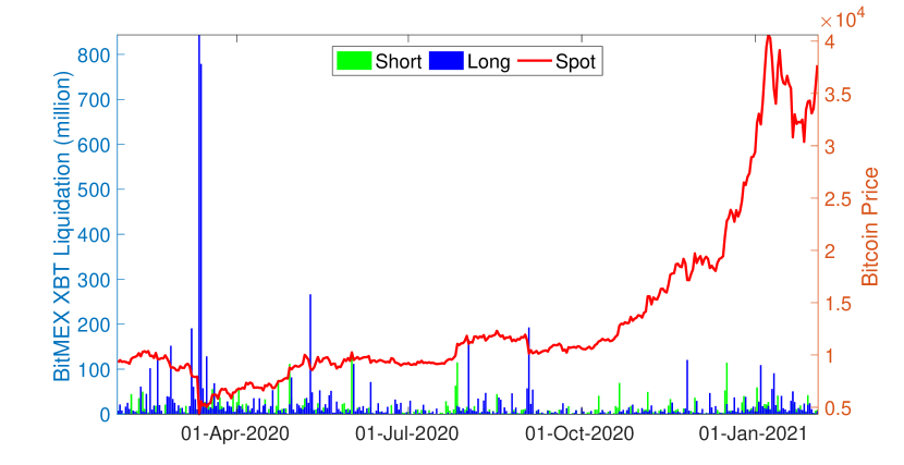
Figure 1: Daily Liquidation Volumes of BitMEX Perpetual Futures

Note: The green (blue) bar plots the forced liquidation of long (short) bitcoin perpetual futures on BitMEX from Jan. 2020 to Feb. 2021. On “Black Thursday” March 12, 2020, the long position’s daily forced liquidation reached 843 million USD. The maximal short liquidation 132 million occurred on June 1, 2020 when the price rise over 10%. The average daily liquidations are around 20 million USD and 10 million USD for long and short. The right y-axis corresponds to the daily bitcoin spot price (red line). The data is manually collected from coinalyze.

This article contributes to the literature in several ways. First, by using daily forced liquidation data of BitMEX, we highlight the speculative activity, aggressiveness and risk preference of market participants by estimating the speculation index, the average percentage of liquidation and average leverages used in long and short positions. Second, we show that generalized extreme value theory (GEV) can effectively capture the bitcoin futures price’s fat-tail feature. Finally, we give optimal margins for long and short positions using GEV and market data that provide guidance for exchanges to design bitcoin futures specifications, especially margin requirements.

With bitcoin perpetual futures data from BitMEX, our empirical analysis uncovered several interesting aspects of bitcoin futures markets. First, The average speculation index sits at 3.75 which is much larger than S&P 500 (0.15), Nikkei (0.21) and DAX (0.45). This shows the extreme speculation activity in BitMEX perpetual market. Second, the daily average percentage of forced liquidation for long and short positions are substantial at levels of 3.51% and 1.89%, respectively. Despite those statistics, the average leverage of those got forced liquidation is similar (around 60X) for both positions. That suggests some participants do trade aggressively and utilize high leverages regardless of high price risk. Third, assuming 1% daily margin call probability, the optimal margins are approximate 33% (3X leverage) for long position and 20% (5X leverage) for short. At last, the GEV distribution is critical for accurately estimating those margins as the normal distribution assumption on return significantly underestimates margin levels by at least 50%.

We organize the rest of the paper as follows. Section 2 introduces bitcoin perpetual futures and generalized extreme value theory. Empirical analysis using BitMEX perpetual futures is conducted in Section 3. Section 4 studies speculation, leverage and liquidation on BitMEX. Section 5 concludes the paper and an appendix collects tables and figures.

2 Bitcoin Perpetual Futures and Extreme Value Theory

2.1 Bitcoin Perpetual Futures

Two types of futures contracts are traded across exchanges: standard futures on CME and Bakkt and perpetual futures (perpetuals) without expiry date on BitMEX, Binance, and Huobi, to name a few. Perpetual futures depart from standard futures in two aspects. Firstly, bitcoin perpetuals are quoted in US dollars (USD) and settled in Bitcoin (XBT); while bitcoin standard futures are both quoted and settled in USD. For instance, each CME bitcoin standard futures contract has a notional value of 5 XBT, while one BitMEX bitcoin perpetual futures has a notional value of 1 USD. Secondly, the bitcoin margin deposit is required for trading perpetuals; while the USD margin is used for standard futures. Since perpetuals account for around 90% trading volume, we only focus on perpetuals here.

Specifically, suppose an investor who enters into one long position of bitcoin perpetual futures with a fixed notional amount of $\Pi$ USD at time $t_{1}$, and closes her position at later time $t_{2}$. The perpetuals prices, denominated in USD, changed from $F_{t_{1}}$ at time $t_{1}$ to $F_{t_{2}}$ at time $t_{2}$. This is equivalent to the change from $\frac{\Pi}{F_{t_{1}}}$ XBT to $\frac{\Pi}{F_{t_{2}}}$ XBT for each perpetuals. Then, the realized pay-off in XBT is given by the difference between the “enter value” and “exit value”:

$$\textit{Long Pay-off}=\frac{\Pi}{F_{t_{1}}}-\frac{\Pi}{F_{t_{2}}}.$$ (2.1)

As a result, the pay-off is inversely related to quotes and perpetuals are also called “inverse” futures. The gain increases when futures price increases as standard futures. However, the magnitude is significantly different from the latter. Similarly, for the short position, the pay-off in XBT is

$$\textit{Short Pay-off}=\frac{\Pi}{F_{t_{2}}}-\frac{\Pi}{F_{t_{1}}}.$$ (2.2)

Implied by equations (2.1) and (2.2), long positions incur greater loss than short positions for the same magnitude of price change $\Delta F$. As a result, margins for long and short would be asymmetric even the perpetuals price ($F_{t}$) fluctuates symmetrically. Empirical results in Section 3 confirm the asymmetry.

2.2 Extreme Value Theory and Optimal Margin

Let $\Delta F_{t_{1}},\Delta F_{t_{2}},\cdots,\Delta F_{t_{n}}$ be quote price changes observed on discrete time $t_{i}=1,2,\cdots,n$. The maximum and minimum changes over $n$ periods are $\textbf{Max}(n)=\max(\Delta F_{t_{1}},\Delta F_{t_{2}},\cdots,\Delta F_{t_{n}})$ and $\textbf{Min}(n)=\min(\Delta F_{t_{1}},\Delta F_{t_{2}},\cdots,\Delta F_{t_{n}})$, respectively. For a wide range of possible distributions of price changes $(\Delta F_{t_{i}})$, the limit distributions of $\textbf{Max}(n)$ and $\textbf{Min}(n)$ follow the generalized extreme value distribution (GEV), see Jenkinson, (1955). The extreme distribution is characterized by location parameter $\mu$, scale parameter $\sigma$, and tail parameter $\tau$. Due to possible asymmetry in left and right tails, GEV parameters could be different for $\textbf{Max}(n)$ and $\textbf{Min}(n)$ in equations (2.3) and (2.4).

$$G_{max}(x) =\mathrm{exp}\left[-\left(1-\frac{x-\mu^{max}}{\sigma^{max}}\cdot\tau^{max}\right)^{1/\tau^{max}}\right],\quad\mbox{and}$$ (2.3)

$$G_{min}(x) =1-\mathrm{exp}\left[-\left(1+\frac{x-\mu^{min}}{\sigma^{min}}\cdot\tau^{min}\right)^{1/\tau^{min}}\right].$$ (2.4)

The introduction of GEV to study optimal margin can be traced back to Longin, (1999), which focuses on silver futures traded on COMEX. Recently, Gkillas and Katsiampa, (2018) also used GEV to estimate Value-at-Risk and expected shortfall of several cryptocurrencies.

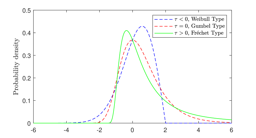
Figure 2: Gumbel, Weibull, and Fr$\acute{e}$chet Distributions

Depending on the tail parameter $\tau$, extreme distributions fall into three categories: Gumbel ($\tau=0$), Weibull ($\tau<0$), and Fr$\acute{e}$chet ($\tau>0$) distributions, which are illustrated in Figure 2.

$<$Insert Figure 2 here.$>$

Over $n$ periods, for a long position, the margin call is triggered once the minimum price change $\textbf{Min}(n)$ is lower than margin deposit $\textbf{MD}_{long}$. Once triggered, the long position would be automatically liquidated if the investor could not pull up enough bitcoin deposit. The corresponding margin call probability, $\textbf{p}^{long}$, is given by

$$\textbf{p}^{long}=\mathbb{P}\mbox{rob}\left(\textbf{Min}(n)<-\textbf{MD}_{long}\right)\simeq G_{min}(-\textbf{MD}_{long}).$$ (2.5)

In parallel, for the short position, we have

$$\textbf{p}^{short}=\mathbb{P}\mbox{rob}\left(\textbf{Max}(n)>\textbf{MD}_{short}\right)\simeq 1-G_{max}(\textbf{MD}_{short}).$$ (2.6)

Using limiting distributions in (2.3) and (2.4), given acceptable margin call probabilities $\textbf{p}^{long}$ and $\textbf{p}^{short}$, minimal margins $\textbf{MD}_{long}$ and $\textbf{MD}_{short}$ can be analytically expressed as

$$\textbf{MD}_{long} =-\mu^{min}+\frac{\sigma^{min}}{\tau^{min}}\left[1-\left(-\ln\left(1-\textbf{p}^{long}\right)\right)^{\tau^{min}}\right],\qquad\mbox{and}$$ (2.7)

$$\textbf{MD}_{short} =\mu^{max}+\frac{\sigma^{max}}{\tau^{max}}\left[1-\left(-\ln\left(1-\textbf{p}^{short}\right)\right)^{\tau^{max}}\right].$$ (2.8)

In Section 3 below, we conduct empirical analysis to estimate left and right GEV distribution parameters $(\tau^{min},\mu^{min},\sigma^{min})$ and $(\tau^{max},\mu^{max},\sigma^{max})$ and related long and short margin levels $\textbf{MD}_{long}$ and $\textbf{MD}_{short}$.

3 Data and Empirical Analysis

3.1 Data Description

The BitMEX exchange, founded in 2014, is the largest online platform for trading bitcoin futures, which runs continuously 24/7 a week and offers various cryptocurrency futures contracts, such as Bitcoin and Ethereum. On BitMEX, both perpetuals and fixed expiration futures are listed. The perpetual futures contracts dominate the market by contributing 90% of the total trading volume. Perpetuals traded on BitMEX have notional value $\Pi=1$ USD and the maximum leverage allowed is 100X (margin requirement is 1%).

To investigate the average leverage used by market participants, we manually collect the daily volume, forced liquidation, open interest and daily OHLC prices (open, high, low, close) data from Coinalyze. The data spans from January 29, 2020 to February 3, 2021 and contains 372 entries. Besides, we also download 5min BitMEX perpetual futures price data using the API provided by BitMEX to investigate optimal margins. The BitMEX perpetual data-set consists of 431, 346 observations from January 1, 2017 to February 6, 2021.

Following Longin, (1999), price changes for perpetual futures are defined in percentage changes $\Delta\widehat{F}_{t}=\frac{\frac{1}{F_{t-1}}-\frac{1}{F_{t}}}{\frac{1}{F_{t-1}}}=1-\frac{{F}_{t-1}}{{F}_{t}}$. This definition has the advantage of being a stationary time series and numéraire independent. Margin level is in terms of percentage. Its left (right) tail is associated with the loss of a long (short) position. We also define an alternative price change as $\Delta{F}_{t}=\frac{F_{t}-F_{t-1}}{F_{t-1}}=\frac{{F}_{t}}{{F}_{t-1}}-1$ if the investor trades USD settled standard bitcoin futures. The difference in optimal margins under two definitions highlights the impact of perpetuals’ inverse pay-off structure.

$<$Insert Table 1 here.$>$

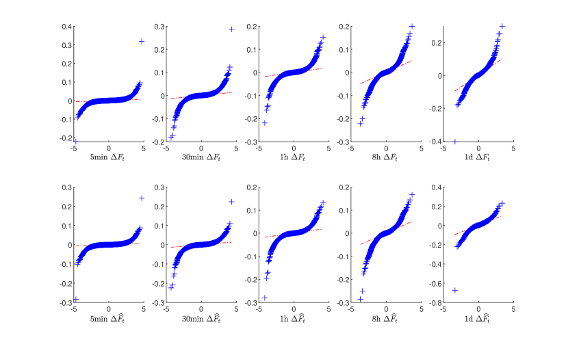
Figure 3: Q-Q Plot of Price Changes $\Delta F$ and $\Delta\widehat{F}$ on BitMEX

Table 1 reports the summary statistics of price changes $\Delta F$ and $\Delta\widehat{F}$, sampled at different frequencies. On daily frequency, both price changes are negatively skewed and leptokurtic, and the magnitude for perpetuals is higher, evidenced by a more negative skewness (-3.67 vs. -0.24). The price change distribution for perpetuals favors the short position than the long position as $\Delta\widehat{F}$ has a lower minimum (-82.67% vs. -45.26%), a lower maximum (22.00% vs. 28.20%) and, as a result, a lower mean (0.14% vs. 0.35%) as well as a thicker tail. These facts are also confirmed by the Q-Q plot in Figure 3.

$<$Insert Figure 3 here.$>$

3.2 GEV Parameter Estimation

As mentioned above, the left/right tail is directly linked to the loss of long/short position. Two sets of parameters $(\mu,\sigma,\tau)$ are estimated separately.

As there is only one extreme value for the full sample, estimating GEV distribution parameters often relies on the block extreme technique. Here, we follow the estimation procedure of Longin, (1999). The technique divides the whole sample into non-overlapping sub-samples containing $n$ observations, and each sub-sample provides us a maximum change and a minimum change. For the $i$-th block $\{\Delta X_{(i-1)n+1},\Delta X_{(i-1)n+2},\cdots,\Delta X_{in}\}$ ($X=\widehat{F}$ and $F$, respectively), we denote the block maximum and minimum as $\min_{i}$ and $\max_{i}$. If we have a total of $N$ observations, the block extreme sets $\{\min_{1},...,\min_{[N/n]}\}$ and $\{\max_{1},...,\max_{[N/n]}\}$ are used to estimate GEV parameters. For different sampling frequencies, the block size $n$ varies. In particular, the block spans 8/24/48 hours for 5/30/60 min sampling and 5/10 days for 8/24 hours sampling frequencies, and we point out the sampling frequency could be treated as the screening-frequency that exchanges/investors monitor the futures positions. We report the corresponding results in Table 2.

The tail parameter $\tau$ is consistently positive, indicating extreme distributions are all Fr$\acute{e}$chet types. The magnitude of $\tau$ increases as the sampling frequency increases, which means the tail is thicker for high-frequency returns. On the other hand, the location and scale parameters are higher for low-frequency returns as extreme price changes increase for longer horizons. Slight differences are observed for left and right tail parameters of standard futures $\Delta F$. However, for perpetual futures $\Delta\widehat{F}_{t}$, the tail parameter $\tau$’s differ significantly for left and right tails, especially for low-frequency cases such as 8h (8 hours) and 1d (1 day). For daily return, the left tail parameter $\tau$ is more than double of the right, and this indicates a fatter left tail (higher risk for the long position).

$<$Insert Table 2 here.$>$

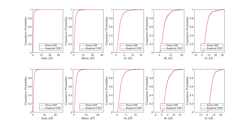
Figure 4: Empirical and Fitted Right Tail CDF of $\Delta F_{t}$ and $\Delta\widehat{F}_{t}$

Finally, we plot the empirical and fitted cumulative distribution functions (CDFs) for both $\Delta F_{t}$ and $\Delta\widehat{F}_{t}$ in Figure 4. Results suggest that the GEV method is suitable for capturing tail behaviors and investigating optimal margins for bitcoin futures.

$<$Insert Figure 4 here.$>$

3.3 Optimal Margin

In this section, using estimated parameters in Table 2 of Section 3.2, we calculate optimal margins via (2.7) and (2.8) and present empirical results in Table 3. Four margin call probabilities and five holding periods are discussed. Both perpetual futures and standard futures are studied to illustrate the impact of the inverse feature on margin requirements. The results for standard futures also provide guidelines for bitcoin futures traded on CME and Bakkt. Moreover, to match the current margin requirements set by exchanges, we also calculate the one common optimal margin level for both positions by simultaneously encompassing the left and right tails. For each case, we also provide the optimal margin based on the normal distribution assumption (in parentheses) to show the importance of GEV distribution.

$<$Insert Table 3 here.$>$

For each holding period, as expected, the optimal margin increases with the decreasing margin call tolerance. For standard futures, the margin increases from 7.86% (7.66%) to 32.95% (35.93%) for short (long) position when margin call probability varies from $p=0.1$ to $p=0.001$; while perpetual futures margin increases from 7.26% (8.36%) to 26.34% (46.98%) accordingly for 8 hours holding period.

The difference in optimal margin levels for different positions is smaller when the margin call tolerance is higher. For different kinds of futures, the standard one has a rather balanced margin requirement for both positions, while the perpetuals require a higher margin for long than short, especially for longer holding periods and lower tolerance of margin calls. The suggested margin for 8 hours holding period is almost doubled for the long than the short position (46.98% vs. 26.34%) when the margin call probability is limited to 0.001. Such asymmetric effect is the direct result of the difference in tail parameters listed in Table 2.

To match the exchanges’ practice of setting equal margins for both positions, we pool maximums and minimums together as $\{-\min_{1},...,-\min_{[N/n]},\max_{1},...,\max_{[N/n]}\}$ and estimate one set of parameters and the corresponding margin levels in Panel C of Table 3. As expected, the common margin level lies somewhere between the long and short cases. For example, for 8 hours holding period with call probability $p=0.001$, the common margin level for perpetual futures is 34.81%, whereas it is 46.98% for the long position and 26.34% for the short position. Finally, the corresponding optimal margins obtained under the normality assumption of return would significantly underestimate optimal margins by at least half.

In the following section, we quantify the speculation activity, trading aggressiveness and liquidation on BitMEX. It reflects market participants’ risk preference in this highly volatile market.

4 Speculation, Leverage and Liquidation on BitMEX

Previously, we estimated optimal margins for both long and short positions under different monitoring frequencies by using perpetual price data. However, to get a sense of investors’ trading activity and risk preference in the bitcoin futures market, calculating speculation percentage and precise leverages used by investors requires traders’ account-level data, which is unavailable from the exchange. Fortunately, Coinalyze reports the forced liquidation of both long and short. Combined with the daily OHLC prices (open, high, low, close) of bitcoin perpetual futures and trading volume and open interest, we can roughly estimate speculation activity and the leverage used by investors who experienced forced liquidation within a particular day.

First, following Garcia et al., (1986), Lucia and Pardo, (2010), and Kim, (2015), we define the speculation index as the ratio of daily trading volume to daily open interest, i.e.

$$\cal{SI}=\frac{\mbox{trading volume}}{\mbox{open interest}}.$$ (4.1)

Intuitively, total trading volume is a proxy for speculation activity and hedging demand is represented by open interest. A lower ratio implies lower speculative activity relative to hedging demand, or vise versa.

Second, we estimate leverage using liquidation data. At time $t$, suppose the futures price is $F_{t}$ (USD) and an investor enters one long (short) position with leverage ${\mathcal{L}}_{long}$ (${\mathcal{L}}_{short}$). The margin required in XBT is $\frac{1}{\mathcal{L}_{long}}\frac{1}{F_{t}}$ for long position and $\frac{1}{\mathcal{L}_{short}}\frac{1}{F_{t}}$ for short position. According to long and short pay-offs in (2.1) and (2.2), at a later time $s$, margin call is triggered once the trading loss wipes out margin deposit, i.e.,

$$\frac{1}{F_{s}}-\frac{1}{F_{t}}=\frac{1}{{\cal L}_{long}}\frac{1}{F_{t}},\quad\mbox{and}\quad\frac{1}{F_{t}}-\frac{1}{F_{s}}=\frac{1}{{\cal L}_{short}}\frac{1}{F_{t}}.$$ (4.2)

As Coinaylze does not report the exact time when each forced liquidation happens, we made further assumption that investors open their positions at the opening of day $d$ and the possible forced liquidation happens when the perpetuals price hits the daily low (high) for the long (short) position on day $d$. The corresponding returns are:

$$r_{d}^{max}=\frac{F_{d}^{high}-F_{d}^{open}}{F_{d}^{open}},\quad\mbox{and}\quad r_{d}^{min}=\frac{F_{d}^{low}-F_{d}^{open}}{F_{d}^{open}}.$$ (4.3)

Here, $F_{d}^{open}$, $F_{d}^{high}$ and $F_{d}^{low}$ stand for the open, high, and low prices. Once got forced liquidation, we could infer traders’ minimal long and short leverages via (4.2) as

$${\cal L}_{long}=-\frac{1+r_{d}^{min}}{r_{d}^{min}},\quad\mbox{and}\quad{\cal L}_{short}=\frac{1+r_{d}^{max}}{r_{d}^{max}}.$$ (4.4)

The long (short) liquidation percentage $p_{long}$ ($p_{short}$) is estimated by the proportion of long (short) liquidation to open interest.

$<$Insert Table 4 here.$>$

$<$Insert Figure 5 here.$>$

The summary statistics for maximal and minimal futures returns, speculation index, liquidation percentage, and leverages are presented in Table 4. The average of speculation index sits at 3.75 which is much larger than S&P 500 (0.15), Nikkei (0.21) and DAX (0.45) in Lucia and Pardo, (2010). Figure 5 plots its time series in the sample period and shows more speculative trades in both bullish and bearish markets. This reflects extreme speculative activity in bitcoin futures market. The daily average percentages of long and short liquidation to open interest are 3.51% and 1.89%, and the average leverage used by those got forced liquidation is at least 58.13X for long and 59.94X for short. This shows liquidation is substantial due to high spot price risk and some investors’ aggressive leverage.

5 Conclusion

It is crucial and of self-interest for exchanges keeping futures margins at a proper level: high enough to preserve market integrity yet low enough to attract broad participants and maintain market liquidity. This paper employed the generalized extreme value theory to address optimal margins for bitcoin futures. Using the BitMEX perpetual futures, we found: first, average leverages used by forced liquidation traders are 58.13X for long and 59.94X for short for the short position. Second, high leverage leads to substantial forced liquidation, where the daily liquidation percentage is 3.51% for long and 1.89% for short. Third, investors should be more rational and cautious to use leverage in the concurrent high volatile market. We suggest 5X leverage for short and 3X leverage for long if one accepts 1% daily margin call probability. Furthermore, the normality assumption of return will significantly underestimate margin levels by at least half.

The policy implications of our results are: (1) exchanges should give more clear documentation of the asymmetric risk character of perpetuals to market participants; (2) exchanges should also consider perpetuals’ inverse-payoff structure and set higher margin for long positions than shorts; (3) it is necessary and important for exchanges to limit leverage allowed and impose more margin deposit to lower forced liquidation, maintain market integrity, and improve the functioning of futures markets.

Appendix

Figures

Note: We consider three tail parameters $\tau=0.5,0,-0.5$. The Fr$\acute{e}$chet distribution (green line) is fat-tailed as its tail is slowly decreasing; the Gumbel distribution (red line) is thin-tailed as its tail is rapidly decreasing; and the Weibull (blue line) has no tail after a certain point.

Note: This figure shows the empirical and fitted CDF of $\Delta F_{t}$ and $\Delta\widehat{F}_{t}$ under 5min, 30min, 1h, 8h, and 1d observation frequencies. All the fitted right tail CDF’s are computed by (2.3) with parameters in Panel A of Table 2.

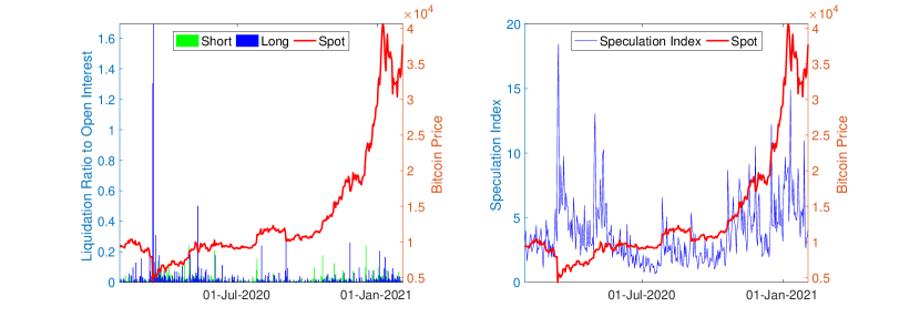
Figure 5: Liquidation Ratio and Speculation Index

Note. The speculation index is defined as the ratio of trading volume to open interest, $\cal{SI}=\frac{\mbox{trading volume}}{\mbox{open interest}}.$ A lower ratio implies lower speculative activity relative to hedging demand.

Tables

Variable	Standard Futures $\Delta F$					Perpetuals $\Delta\widehat{F}$
$t$	5min	30min	1h	8h	1d		5min	30min	1h	8h	1d
Min	$-$0.2230	$-$0.1671	$-$0.2514	$-$0.2902	$-$0.4526		$-$0.2870	$-$0.2006	$-$0.3358	$-$0.4088	$-$0.8267
P25	$-$0.0008	$-$0.0020	$-$0.0027	$-$0.0079	$-$0.0146		$-$0.0008	$-$0.0020	$-$0.0027	$-$0.0080	$-$0.0148
Median	0.0000	0.0001	0.0001	0.0008	0.0027		0.0000	0.0001	0.0001	0.0008	0.0027
Mean	0.0000	0.0001	0.0002	0.0012	0.0035		0.0000	0.0000	0.0001	0.0005	0.0014
P75	0.0009	0.0022	0.0031	0.0108	0.0223		0.0009	0.0022	0.0031	0.0106	0.0218
Max	0.3190	0.2396	0.1440	0.2333	0.2820		0.2419	0.1933	0.1259	0.1892	0.2200
Skewness	1.5741	0.0689	$-$0.5213	$-$0.0481	$-$0.2415		$-$1.6286	$-$1.1195	$-$1.9050	$-$1.3412	$-$3.6652
Kurtosis	434.28	61.44	39.27	15.35	14.10		358.63	59.91	68.47	24.75	65.36
S.D.	0.0030	0.0069	0.0096	0.0253	0.0446		0.0030	0.0069	0.0097	0.0257	0.0476
Nobs	431346	71891	35945	4493	1497		431346	71891	35945	4493	1497
Stationary	Yes	Yes	Yes	Yes	Yes		Yes	Yes	Yes	Yes	Yes

Table 1: Summary Statistics of Price Changes $\Delta F$ and $\Delta\widehat{F}$ on BitMEX

Note. It reports summary statistics of price changes $\Delta F$ and $\Delta\widehat{F}$ using BitMEX perpetual futures from January 1, 2017, to February 6, 2021, sampled at 5min, 30min, 1h, 8h, and 1d frequencies. P25 and P75 refer to 25% and 75% quantiles, and S.D. is the standard deviation.

Variable	Standard Futures $\Delta F$					Perpetuals $\Delta\widehat{F}$
$t$	5min	30min	1h	8h	1d		5min	30min	1h	8h	1d
Panel A: Right Tail
$\tau$	0.3939	0.3643	0.3163	0.2386	0.2097		0.3845	0.3455	0.2904	0.1948	0.1424
	(0.0147)	(0.0268)	(0.0362)	(0.0517)	(0.0731)		(0.0147)	(0.0267)	(0.0359)	(0.0507)	(0.0713)
$\sigma$	0.2967	0.6119	0.9078	1.7176	2.8115		0.2938	0.6003	0.8817	1.6229	2.5662
	(0.0046)	(0.0163)	(0.0330)	(0.0929)	(0.2127)		(0.0045)	(0.0158)	(0.0316)	(0.0857)	(0.1877)
$\mu$	0.4281	0.8947	1.3809	2.7411	4.5184		0.4265	0.8879	1.3642	2.6731	4.3345
	(0.0051)	(0.0185)	(0.0387)	(0.1141)	(0.2648)		(0.0051)	(0.0182)	(0.0376)	(0.1078)	(0.2415)
Panel B: Left Tail
$\tau$	0.4389	0.4112	0.3326	0.2641	0.2261		0.4490	0.4311	0.3620	0.3152	0.3102
	(0.0156)	(0.0278)	(0.0391)	(0.0568)	(0.0785)		(0.0156)	(0.0278)	(0.0392)	(0.0577)	(0.0811)
$\sigma$	0.3057	0.6173	0.9149	1.7020	2.6053		0.3087	0.6294	0.9414	1.7928	2.8165
	(0.0049)	(0.0170)	(0.0342)	(0.0954)	(0.2027)		(0.0050)	(0.0175)	(0.0358)	(0.1033)	(0.2293)
$\mu$	0.4276	0.8704	1.3417	2.4324	3.6979		0.4291	0.8768	1.3568	2.4840	3.8108
	(0.0053)	(0.0188)	(0.0396)	(0.1149)	(0.2491)		(0.0054)	(0.0191)	(0.0407)	(0.1210)	(0.2695)
Panel C: Common Tail
$\tau$	0.4165	0.3876	0.3237	0.2447	0.2096		0.4176	0.3901	0.3272	0.2531	0.2255
	(0.0107)	(0.0193)	(0.0266)	(0.0380)	(0.0528)		(0.0107)	(0.0193)	(0.0265)	(0.0378)	(0.0511)
$\sigma$	0.3012	0.6149	0.9121	1.7242	2.7480		0.3012	0.6148	0.9118	1.7197	2.7270
	(0.0033)	(0.0118)	(0.0238)	(0.0668)	(0.1480)		(0.0033)	(0.0118)	(0.0238)	(0.0668)	(0.1470)
$\mu$	0.4278	0.8825	1.3616	2.5891	4.1036		0.4277	0.8819	1.3601	2.5805	4.0740
	(0.0037)	(0.0132)	(0.0277)	(0.0816)	(0.1840)		(0.0037)	(0.0132)	(0.0277)	(0.0812)	(0.1815)

Table 2: GEV Parameter Estimations for $\Delta F$ and $\Delta\widehat{F}$

Note: This table reports left and right tail parameter estimations for $\Delta F$ and $\Delta\widehat{F}$ under 5min, 30min, 1h, 8h, and 1d observation frequencies. For comparison purposes, we take the absolute value of the left tail to estimate corresponding extreme parameters and report a common tail that simultaneously encompasses absolute left tail and right tail. Since variables $\Delta F_{t}$ and $\Delta\widehat{F}_{t}$ are quite small, we multiply them by 100. The corresponding standard errors are included in parentheses.

Table 3: Optimal Margins for Bitcoin Standard Futures and Perpetual Futures

	Standard Futures Margin (%)					Perpetual Futures Margin (%)
Margin Call Probability	0.1	0.05	0.01	0.001		0.1	0.05	0.01	0.001
Panel A: Short Position
5min	1.50	2.10	4.29	11.12		1.48	2.06	4.14	10.54
	(0.38)	(0.49)	(0.69)	(0.92)		(0.38)	(0.49)	(0.69)	(0.92)
30min	3.03	4.17	8.19	20.01		2.93	4.00	7.67	18.05
	(0.88)	(1.13)	(1.60)	(2.13)		(0.89)	(1.14)	(1.61)	(2.14)
1h	4.36	5.85	10.81	24.02		4.16	5.52	9.88	20.89
	(1.21)	(1.56)	(2.21)	(2.94)		(1.23)	(1.59)	(2.24)	(2.98)
8h	7.86	10.17	17.12	32.95		7.26	9.20	14.76	26.34
	(3.13)	(4.05)	(5.77)	(7.70)		(3.24)	(4.17)	(5.92)	(7.88)
1d	12.60	16.11	26.29	48.19		11.14	13.82	21.01	34.50
	(5.37)	(6.99)	(10.02)	(13.43)		(5.96)	(7.69)	(10.94)	(14.58)
Panel B: Long Position
5min	1.60	2.30	4.98	14.17		1.63	2.35	5.17	15.03
	(0.38)	(0.49)	(0.69)	(0.92)		(0.38)	(0.49)	(0.69)	(0.92)
30min	3.16	4.46	9.32	25.07		3.27	4.67	10.03	28.10
	(0.89)	(1.14)	(1.61)	(2.14)		(0.89)	(1.14)	(1.61)	(2.14)
1h	4.41	5.98	11.30	25.96		4.63	6.38	12.50	30.45
	(1.24)	(1.59)	(2.24)	(2.97)		(1.25)	(1.60)	(2.26)	(3.00)
8h	7.66	10.11	17.71	35.93		8.36	11.30	21.05	46.98
	(3.36)	(4.28)	(6.00)	(7.93)		(3.34)	(4.27)	(6.02)	(7.99)
1d	11.34	14.73	24.78	47.11		12.98	17.55	32.56	72.10
	(6.06)	(7.68)	(10.72)	(14.12)		(6.24)	(7.97)	(11.22)	(14.86)
Panel C: Common Position
5min	1.55	2.20	4.62	12.55		1.55	2.20	4.63	12.61
30min	3.09	4.31	8.73	22.37		3.10	4.33	8.79	22.63
1h	4.38	5.91	11.03	24.90		4.39	5.94	11.13	25.28
8h	7.76	10.12	17.26	33.74		7.80	10.19	17.55	34.81
1d	12.55	15.88	25.03	42.91		12.07	15.61	26.10	49.39

Note: This table reports optimal margins for Bitcoin standard futures and perpetual futures for short (Panel A) and long (Panel B) positions. The optimal margins for long and short positions are calculated via (2.7) and (2.8). Panel C gives the margin level for the common position. The corresponding optimal margin levels obtained under the assumption of normality are also presented in parentheses, which are calculated via $p^{long}=\frac{1}{\sqrt{2\pi}\sigma}\int_{-\infty}^{-ML^{long}}e^{-(x-\mu)^{2}/2\sigma^{2}}dx$ and $p^{short}=\frac{1}{\sqrt{2\pi}\sigma}\int_{ML^{\text{short }}}^{+\infty}e^{-(x-\mu)^{2}/2\sigma^{2}}dx$. Here, $\mu$ and $\sigma$ are the mean and standard deviation of price changes $\Delta F_{t}$ and $\Delta\widehat{F}_{t}$. $ML_{long}$ and $ML_{short}$ denote optimal margins of long and short positions.

Table 4: Summary Statistics for Speculation, Liquidation and Leverage

Variables	$r_{d}^{min}$	$r_{d}^{max}$	long liq.(M)	short liq.(M)	$\cal{SI}$	$p_{long}(\%)$	$p_{short}(\%)$	${\cal L}_{long}$	${\cal L}_{short}$
min	-0.46	0.00	0.00	0.00	0.66	0.00	0.00	1.16	3.84
median	-0.02	0.02	6.93	4.60	3.12	1.22	0.86	55.97	56.34
mean	-0.03	0.03	20.14	10.17	3.75	3.51	1.89	58.13	59.94
max	0.00	0.35	843.39	132.70	18.42	169.39	24.32	100.00	100.00
Nobs	372	372	372	372	372	372	372	372	372

Note. The maximal and minimal return $r_{d}^{min}$ and $r_{d}^{max}$ are estimated via (4.3). The speculation index is defined as the ratio of trading volume to open interest, $\cal{SI}=\frac{\mbox{trading volume}}{\mbox{open interest}}.$ The long and short liquidation percentage $p_{long}$ and $p_{short}$ are estimated by the proportion of long/short liquidation to open interest. The long and short leverage ${\cal L}_{long}$ and ${\cal L}_{short}$ are estimated via (4.4). All the data is daily frequency from January 29, 2020 to February 3, 2021. M denotes the Million USD.

References

- (1) Alexander, C., Choi, J., Park, H., and Sohn, S. (2020a). Bitmex bitcoin derivatives: Price discovery, informational efficiency, and hedging effectiveness. Journal of Futures Markets, 40(1):23–43.
- (2) Alexander, C., Deng, J., and Zou, B. (2020b). Optimal hedging with margin constraints and default aversion and its application to bitcoin inverse futures markets. Working Paper. Available at SSRN: https://ssrn.com/abstract=3760048.
- Alexander et al., (2019) Alexander, C., Kaeck, A., and Sumawong, A. (2019). A parsimonious parametric model for generating margin requirements for futures. European Journal of Operational Research, 273(1):31–43.
- Chaim and Laurini, (2018) Chaim, P. and Laurini, M. P. (2018). Volatility and return jumps in bitcoin. Economics Letters, 173:158–163.
- Cotter, (2001) Cotter, J. (2001). Margin exceedences for european stock index futures using extreme value theory. Journal of Banking Finance, 25(8):1475–1502.
- Daskalaki and Skiadopoulos, (2016) Daskalaki, C. and Skiadopoulos, G. (2016). The effects of margin changes on commodity futures markets. Journal of Financial Stability, 22:129–152.
- Deng et al., (2019) Deng, J., Pan, H., Zhang, S., and Zou, B. (2019). Optimal bitcoin trading with inverse futures. Available at SSRN 3441913.
- Deng et al., (2020) Deng, J., Pan, H., Zhang, S., and Zou, B. (2020). Minimum-variance hedging of bitcoin inverse futures. Applied Economics, 52:6320–6337.
- Dewachter and Gielens, (1999) Dewachter, H. and Gielens, G. (1999). Setting futures margins: the extremes approach. Applied Financial Economics, 9(2):173–181.
- Figlewski, (1984) Figlewski, S. (1984). Margins and market integrity: Margin setting for stock index futures and options. The Journal of Futures Markets (pre-1986), 4(3):385.
- Garcia et al., (1986) Garcia, P., Leuthold, R. M., and Zapata, H. (1986). Lead-lag relationships between trading volume and price variability: New evidence. The Journal of Futures Markets (1986-1998), 6(1):1.
- Gkillas and Katsiampa, (2018) Gkillas, K. and Katsiampa, P. (2018). An application of extreme value theory to cryptocurrencies. Economics Letters, 164:109–111.
- Jenkinson, (1955) Jenkinson, A. F. (1955). The frequency distribution of the annual maximum (or minimum) values of meteorological elements. Quarterly Journal of the Royal Meteorological Society, 81(348):158–171.
- Kim, (2015) Kim, A. (2015). Does futures speculation destabilize commodity markets? Journal of Futures Markets, 35(8):696–714.
- Longin, (1999) Longin, F. M. (1999). Optimal margin level in futures markets: Extreme price movements. Journal of Futures Markets, 19(2):127–152.
- Lucia and Pardo, (2010) Lucia, J. J. and Pardo, A. (2010). On measuring speculative and hedging activities in futures markets from volume and open interest data. Applied Economics, 42(12):1549–1557.
- Scaillet et al., (2020) Scaillet, O., Treccani, A., and Trevisan, C. (2020). High-frequency jump analysis of the bitcoin market. Journal of Financial Econometrics, 18(2):209–232.
- Sebastião and Godinho, (2020) Sebastião, H. and Godinho, P. (2020). Bitcoin futures: An effective tool for hedging cryptocurrencies. Finance Research Letters, 33:101230.