Tightness and Equivalence of Semidefinite Relaxations for MIMO Detection

Abstract

The multiple-input multiple-output (MIMO) detection problem, a fundamental problem in modern digital communications, is to detect a vector of transmitted symbols from the noisy outputs of a fading MIMO channel. The maximum likelihood detector can be formulated as a complex least-squares problem with discrete variables, which is NP-hard in general. Various semidefinite relaxation (SDR) methods have been proposed in the literature to solve the problem due to their polynomial-time worst-case complexity and good detection error rate performance. In this paper, we consider two popular classes of SDR-based detectors and study the conditions under which the SDRs are tight and the relationship between different SDR models. For the enhanced complex and real SDRs proposed recently by Lu et al., we refine their analysis and derive the necessary and sufficient condition for the complex SDR to be tight, as well as a necessary condition for the real SDR to be tight. In contrast, we also show that another SDR proposed by Mobasher et al. is not tight with high probability under mild conditions. Moreover, we establish a general theorem that shows the equivalence between two subsets of positive semidefinite matrices in different dimensions by exploiting a special “separable” structure in the constraints. Our theorem recovers two existing equivalence results of SDRs defined in different settings and has the potential to find other applications due to its generality.

90C22, 90C20, 90C46, 90C27

1 Introduction

Multiple-input multiple-output (MIMO) detection is a fundamental problem in modern digital communications [33, 36]. The MIMO channel can be modeled as

(1) $${\bm{r}}={\mathbf{H}}{\bm{x}}^{*}+{\bm{v}},$$

where ${\bm{r}}\in\mathbb{C}^{m}$ is the vector of received signals, ${\mathbf{H}}\in\mathbb{C}^{m\times n}$ is a complex channel matrix, ${\bm{x}}^{*}$ is the vector of transmitted symbols, and ${\bm{v}}$ is the vector of additive Gaussian noises. Moreover, each entry of ${\bm{x}}^{*}$ is drawn from a discrete symbol set ${\mathcal{S}}$ determined by the modulation scheme.

The MIMO detection problem is to recover the transmitted symbol vector ${\bm{x}}^{*}$ from the noisy channel output ${\bm{r}}$, with the information of the symbol set ${\mathcal{S}}$ and the channel matrix ${\mathbf{H}}$. Under the assumption that each entry of ${\bm{x}}^{*}$ is drawn uniformly and independently from the symbol set ${\mathcal{S}}$, it is known that the maximum likelihood detector can achieve the optimal detection error rate performance. Mathematically, it can be formulated as a discrete least-squares problem:

(2) $$\min_{{\bm{x}}\in\mathbb{C}^{n}} \|{\mathbf{H}}{\bm{x}}-{\bm{r}}\|_{2}^{2}$$

$$\mathrm{s.t.} x_{i}\in\mathcal{S},\;i=1,2,\ldots,n,$$

where $x_{i}$ denotes the $i$-th entry of the vector ${\bm{x}}$ and $\|\cdot\|_{2}$ denotes the Euclidean norm. In this paper, unless otherwise specified, we will focus on the $M$-ary phase shift keying ($M$-PSK) modulation, whose symbol set is given by

(3) $$\mathcal{S}_{M}:=\bigl{\{}z\in\mathbb{C}:\;|z|=1,\;\mathrm{arg}(z)\in\{2j\pi/M,\;j=0,1,\ldots,M-1\}\bigr{\}},$$

where $|z|$ and $\mathrm{arg}(z)$ denote the modulus and argument of a complex number, respectively. As in most practical digital communication systems, throughout the paper we require $M=2^{b}$ where $b\geq 1$ is an integer.

Many detection algorithms have been proposed to solve problem Eq. 2 either exactly or approximately. However, for general ${\mathbf{H}}$ and ${\bm{r}}$, problem Eq. 2 has been proved to be NP-hard [32]. Hence, no polynomial-time algorithms can find the exact solution (unless $\text{P}=\text{NP}$). Sphere decoding [4], a classical combinatorial algorithm based on the branch-and-bound paradigm, offers an efficient way to solve problem Eq. 2 exactly when the problem size is small, but its expected complexity is still exponential [11]. On the other hand, some suboptimal algorithms such as linear detectors [23, 6] and decision-feedback detectors [35, 5] enjoy low complexity but at the expense of substantial performance loss: see [36] for an excellent review.

Over the past two decades, semidefinite relaxation (SDR) has gained increasing attention in non-convex optimization [7, 18, 34]. It is a celebrated technique to tackle quadratic optimization problems arising from various signal processing and wireless communication applications, such as beamforming design [24, 15], sensor network localization [3, 2, 27], and angular synchronization [25, 1, 37]. Such SDR-based approaches can usually offer superior performance in both theory and practice while maintaining polynomial-time worst-case complexity.

For MIMO detection problem Eq. 2, the first SDR detector [30, 20] was designed for the real MIMO channel and the binary symbol set $\mathcal{S}=\{+1,-1\}$. Notably, it is proved that this detector can achieve the maximal possible diversity order [12], meaning that it achieves an asymptotically optimal detection error rate when the signal-to-noise ratio (SNR) is high. It was later extended to the more general setting with a complex channel and an $M$-PSK symbol set in [28, 19], which we refer to as the conventional SDR or Eq. CSDR. However, this conventional approach fails to fully utilize the structure in the symbol set $\mathcal{S}$. To overcome this issue, researchers have developed various improved SDRs and we consider the two most popular classes below. The first class proposed in [22] is based on an equivalent zero-one integer programming formulation of problem Eq. 2. Four SDR models were introduced and two of them will be discussed in details later (see Eq. ESDR1-${\mathbf{T}}$ and Eq. ESDR2-${\mathbf{T}}$ further ahead). The second class proposed in [17] further enhances Eq. CSDR by adding valid cuts, resulting in a complex SDR and a real SDR (see Eq. ESDR-${\mathbf{X}}$ and Eq. ESDR-${\mathbf{Y}}$ later on).

In this paper, we focus on two key problems in SDR-based MIMO detection: the tightness of SDRs and the relationship between different SDR models. Firstly, note that SDR detectors are suboptimal algorithms as they replace the original discrete optimization problem Eq. 2 with tractable semidefinite programs (SDPs). Hence, after solving an SDP, we need some rounding procedure to make final symbol decisions. However, under some favorable conditions on ${\mathbf{H}}$ and ${\bm{v}}$, an SDR can be tight, i.e., it has an optimal rank-one solution corresponding to the true vector of transmitted symbols. Such tightness conditions are of great interest since they give theoretical guarantees on the optimality of SDR detectors. While it has been well studied for the simple case [9, 10, 14, 26] where ${\mathbf{H}}\in\mathbb{R}^{m\times n}$, ${\bm{v}}\in\mathbb{R}^{m}$, and $\mathcal{S}=\{+1,-1\}$, for the more general case where ${\mathbf{H}}\in\mathbb{C}^{m\times n}$, ${\bm{v}}\in\mathbb{C}^{m}$, and $\mathcal{S}=\mathcal{S}_{M}$ ($M\geq 4$), tightness conditions for SDR detectors have remained unknown until very recently. The authors in [17] showed that Eq. CSDR is not tight with probability one under some mild conditions. On the other hand, their proposed enhanced SDRs are tight if the following condition is satisfied:

(4) $$\lambda_{\mathrm{min}}({\mathbf{H}}^{\dagger}{\mathbf{H}})\sin\left(\frac{\pi}{M}\right)>\|{\mathbf{H}}^{\dagger}{\bm{v}}\|_{\infty},$$

where $\lambda_{\mathrm{min}}(\cdot)$ denotes the smallest eigenvalue of a matrix, $(\cdot)^{\dagger}$ denotes the conjugate transpose, and $\|\cdot\|_{\infty}$ denotes the $L_{\infty}$-norm. To the best of our knowledge, this is the best condition that guarantees a certain SDR to be tight for problem Eq. 2 in the $M$-PSK settings.

Secondly, researchers have noticed some rather unexpected equivalence between different SDR models independently developed in the literature. The earliest one of such results is reported in [21], where three different SDRs for the high-order quadrature amplitude modulation (QAM) symbol sets are proved to be equivalent. Very recently, the authors in [16] showed that the enhanced real SDR proposed in [17] is equivalent to one SDR model in [22]. It is worth noting that while these two papers are of the same nature, the proof techniques are quite different and it is unclear how to generalize their results at present.

In this paper, we make contributions to both problems. For the tightness of SDRs, we sharpen the analysis in [17] to give the necessary and sufficient condition for the complex enhanced SDR to be tight, and a necessary condition for the real enhanced SDR to be tight. Specifically, for the case where $M\geq 4$, we show that the enhanced complex SDR Eq. ESDR-${\mathbf{X}}$ is tight if and only if

(5) $${\mathbf{H}}^{\dagger}{\mathbf{H}}+{\mathrm{Diag}}\big{(}\mathrm{Re}({\mathrm{Diag}}({\bm{x}}^{*})^{-1}{\mathbf{H}}^{\dagger}{\bm{v}})\big{)}-\cot\left(\frac{\pi}{M}\right){\mathrm{Diag}}(|\mathrm{Im}({\mathrm{Diag}}({\bm{x}}^{*})^{-1}{\mathbf{H}}^{\dagger}{\bm{v}})|\big{)}\succeq 0,$$

while the enhanced real SDR Eq. ESDR-${\mathbf{Y}}$ is tight only if

(6) $${\mathbf{H}}^{\dagger}{\mathbf{H}}+{\mathrm{Diag}}\big{(}\mathrm{Re}({\mathrm{Diag}}({\bm{x}}^{*})^{-1}{\mathbf{H}}^{\dagger}{\bm{v}})\big{)}-\cot\left(\frac{2\pi}{M}\right){\mathrm{Diag}}(|\mathrm{Im}({\mathrm{Diag}}({\bm{x}}^{*})^{-1}{\mathbf{H}}^{\dagger}{\bm{v}})|\big{)}\succeq 0,$$

where ${\mathbf{A}}\succeq 0$ means that the matrix ${\mathbf{A}}$ is positive semidefinite (PSD), ${\mathrm{Diag}}({\bm{x}})$ denotes a diagonal matrix whose diagonals are the vector ${\bm{x}}$, and ${\mathrm{Re}}(\cdot)$, ${\mathrm{Im}}(\cdot)$, and $|\cdot|$ denote the entrywise real part, imaginary part, and absolute value of a number/vector/matrix, respectively. Moreover, we prove that one of the SDR models proposed in [22] is generally not tight: under some mild assumptions, its probability of being tight decays exponentially with respect to the number of transmitted symbols $n$.

For the relationship between different SDR models, we propose a general theorem showing the equivalence between two subsets of PSD cones. Specifically, we prove the correspondence between a subset of a high-dimensional PSD cone with a special “separable” structure and the one in a lower dimension. Our theorem covers both equivalence results in [21] and [16] as special cases, and has the potential to find other applications due to its generality.

The paper is organized as follows. We introduce the existing SDRs for Eq. 2 in Section 2 and analyze their tightness in Section 3. In Section 4, we propose a general theorem that establishes the equivalence between two subsets of PSD cones in different dimensions, and discuss how our theorem implies previous results. Section 5 provides some numerical results to validate our analysis. Finally, Section 6 concludes the paper.

We summarize some standard notations used in this paper. We use $x_{i}$ to denote the $i$-th entry of a vector ${\bm{x}}$ and $X_{i,j}$ to denote the $(i,j)$-th entry of a matrix ${\mathbf{X}}$. We use $|\cdot|$, $\|\cdot\|_{2}$, and $\|\cdot\|_{\infty}$ to denote the entrywise absolute value, the Euclidean norm, and the $L_{\infty}$ norm of a vector, respectively. For a given number/vector/matrix, we use $(\cdot)^{\dagger}$ to denote the conjugate transpose, $(\cdot)^{\mathsf{T}}$ to denote the transpose, and ${\mathrm{Re}}(\cdot)$/${\mathrm{Im}}(\cdot)$ to denote the entrywise real/imaginary part. We use ${\mathrm{Diag}}({\bm{x}})$ to denote the diagonal matrix whose diagonals are the vector ${\bm{x}}$, and $\operatorname{diag}({\mathbf{X}})$ to denote the vector whose entries are the diagonals of the matrix ${\mathbf{X}}$. Given an $m\times n$ matrix ${\mathbf{A}}$ and the index sets $\alpha\subset\{1,2,\ldots,m\}$ and $\beta\subset\{1,2,\ldots,n\}$, we use ${\mathbf{A}}[\alpha,\beta]$ to denote the submatrix with entires in the rows of ${\mathbf{A}}$ indexed by $\alpha$ and the columns indexed by $\beta$. Moreover, we denote the principal submatrix ${\mathbf{A}}[\alpha,\alpha]$ by ${\mathbf{A}}[\alpha]$ in short. For two matrices ${\mathbf{A}}$ and ${\mathbf{B}}$ of appropriate size, $\langle{\mathbf{A}},{\mathbf{B}}\rangle:={\mathrm{Re}}(\mathrm{Tr}({\mathbf{A}}^{\dagger}{\mathbf{B}}))$ denotes the inner product, ${\mathbf{A}}\otimes{\mathbf{B}}$ denotes the Kronecker product, and ${\mathbf{A}}\succeq{\mathbf{B}}$ means ${\mathbf{A}}-{\mathbf{B}}$ is PSD. For a set $\mathcal{A}$ in a vector space, we use $\mathrm{conv}(\mathcal{A})$ to denote its convex hull. For a random variable $X$ and measurable sets $\mathcal{B}$ and $\mathcal{C}$, $\mathbf{Prob}(X\in\mathcal{B})$ denotes the probability of the event $\{X\in\mathcal{B}\}$, $\mathbf{Prob}(X\in\mathcal{B}{\>|\>}\mathcal{C})$ denotes the conditional probability given $\mathcal{C}$, and $\operatorname*{\mathbb{E}}[X]$ denotes the expectation of $X$. Finally, the symbols ${\mathbf{i}}$, ${\bm{1}}_{n}$, ${\mathbf{I}}_{n}$, and $\mathbb{S}_{+}^{n}$ represent the imaginary unit, the $n\times 1$ all-one vector, the $n\times n$ identity matrix, and the $n$-dimensional PSD cone, respectively.

2 Review of semidefinite relaxations

In this paper, we focus on the $M$-PSK setting with the symbol set $\mathcal{S}_{M}$ given in Eq. 3. To simplify the notations, we let ${\bm{s}}\in\mathbb{C}^{M}$ be the vector of all symbols, where

$$s_{j}=e^{{\mathbf{i}}\theta_{j}}\;\text{and}\;\theta_{j}=\frac{(j-1)2\pi}{M},\;j=1,2,\ldots,M,$$

and further we let ${\bm{s}}_{R}={\mathrm{Re}}({\bm{s}})$ and ${\bm{s}}_{I}={\mathrm{Im}}({\bm{s}})$.

The objective in Eq. 2 can be written as

$$\|{\mathbf{H}}{\bm{x}}-{\bm{r}}\|_{2}^{2}={\bm{x}}^{\dagger}{\mathbf{Q}}{\bm{x}}+2\mathrm{Re}({\bm{c}}^{\dagger}{\bm{x}})+{\bm{r}}^{\dagger}{\bm{r}}=\langle{\mathbf{Q}},{\bm{x}}{\bm{x}}^{\dagger}\rangle+2\mathrm{Re}({\bm{c}}^{\dagger}{\bm{x}})+{\bm{r}}^{\dagger}{\bm{r}},$$

where we define

(7) $${\mathbf{Q}}={\mathbf{H}}^{\dagger}{\mathbf{H}}\;\text{and}\;{\bm{c}}=-{\mathbf{H}}^{\dagger}{\bm{r}}.$$

By introducing ${\mathbf{X}}={\bm{x}}{\bm{x}}^{\dagger}$ and discarding the constant ${\bm{r}}^{\dagger}{\bm{r}}$, we can reformulate Eq. 2 as

(8) $$\min_{{\bm{x}},{\mathbf{X}}} \langle{\mathbf{Q}},{\mathbf{X}}\rangle+2\mathrm{Re}({\bm{c}}^{\dagger}{\bm{x}})$$

$$\mathrm{s.t.} X_{i,i}=1,\;i=1,2,\ldots,n,$$

$$x_{i}\in\mathcal{S}_{M},\;i=1,2,\ldots,n,$$

$${\mathbf{X}}={\bm{x}}{\bm{x}}^{\dagger},$$

where the constraint $X_{i,i}=1$ comes from $X_{i,i}=|x_{i}|^{2}=1$. The conventional SDR (CSDR) in [28, 19] simply drops the discrete symbol constraints $x_{i}\in\mathcal{S}_{M}$ and relaxes the rank-one constraint to ${\mathbf{X}}\succeq{\bm{x}}{\bm{x}}^{\dagger}$, resulting in the following relaxation:

(CSDR) $$\min_{{\bm{x}},{\mathbf{X}}} \langle{\mathbf{Q}},{\mathbf{X}}\rangle+2\mathrm{Re}({\bm{c}}^{\dagger}{\bm{x}})$$

$$\mathrm{s.t.} X_{i,i}=1,\;i=1,2,\ldots,n,$$

$${\mathbf{X}}\succeq{\bm{x}}{\bm{x}}^{\dagger},$$

where ${\bm{x}}\in\mathbb{C}^{n}$ and ${\mathbf{X}}\in\mathbb{C}^{n\times n}$. Since ${\mathbf{X}}\succeq{\bm{x}}{\bm{x}}^{\dagger}$ is equivalent to

$$\begin{bmatrix}1&{\bm{x}}^{\dagger}\\ {\bm{x}}&{\mathbf{X}}\end{bmatrix}\succeq 0,$$

the above Eq. CSDR is an SDP on the complex domain. Moreover, for the simple case where ${\mathbf{H}}\in\mathbb{R}^{m\times n}$, ${\bm{v}}\in\mathbb{R}^{m}$, and $M=2$, a real SDR similar to Eq. CSDR has the form:

(9) $$\min_{{\bm{x}},{\mathbf{X}}} \langle{\mathbf{Q}},{\mathbf{X}}\rangle+2{\bm{c}}^{\mathsf{T}}{\bm{x}}$$

$$\mathrm{s.t.} X_{i,i}=1,\;i=1,2,\ldots,n,$$

$${\mathbf{X}}\succeq{\bm{x}}{\bm{x}}^{\mathsf{T}},$$

where ${\bm{x}}\in\mathbb{R}^{n}$, ${\mathbf{X}}\in\mathbb{R}^{n\times n}$, and we redefine ${\mathbf{Q}}={\mathbf{H}}^{\mathsf{T}}{\mathbf{H}}$ and ${\bm{c}}=-{\mathbf{H}}^{\mathsf{T}}{\bm{r}}$ (cf. Eq. 7). The problem Eq. 9 has also been extensively studied in the literature [30, 20, 9, 10, 14, 26]. It is proved in [9, 10] that Eq. 9 is tight if and only if

(10) $${\mathbf{H}}^{\mathsf{T}}{\mathbf{H}}+[{\mathrm{Diag}}({\bm{x}}^{*})]^{-1}{\mathrm{Diag}}({\mathbf{H}}^{\mathsf{T}}{\bm{v}})\succeq 0,$$

while Eq. CSDR is not tight for $M\geq 4$ with probability one under some mild conditions [17].

Recently, a class of enhanced SDRs was proposed in [17]. Instead of simply dropping the constraints $x_{i}\in{\mathcal{S}}_{M}$ as in Eq. CSDR, the authors replaced the discrete symbol set ${\mathcal{S}}_{M}$ by its convex hull to get a continuous relaxation:

(ESDR-$${\mathbf{X}} \min_{{\bm{t}},{\bm{x}},{\mathbf{X}}} \langle{\mathbf{Q}},{\mathbf{X}}\rangle+2\mathrm{Re}({\bm{c}}^{\dagger}{\bm{x}})$$)

$$\mathrm{s.t.} X_{i,i}=1,\;i=1,2,\ldots,n,$$

$$x_{i}=\sum_{j=1}^{M}t_{i,j}s_{j},\;\sum_{j=1}^{M}t_{i,j}=1,\;i=1,2,\ldots,n,$$

$$t_{i,j}\geq 0,\;j=1,2,\ldots,M,\;i=1,2,\ldots,n,$$

$${\mathbf{X}}\succeq{\bm{x}}{\bm{x}}^{\dagger},$$

where ${\bm{x}}\in\mathbb{C}^{n}$, ${\mathbf{X}}\in\mathbb{C}^{n\times n}$, and ${\bm{t}}\in\mathbb{R}^{Mn}$ is the concatenation of $M$-dimensional vectors ${\bm{t}}_{1},{\bm{t}}_{2},\ldots,{\bm{t}}_{n}$ with ${\bm{t}}_{i}=[t_{i,1},t_{i,2},\ldots,t_{i,M}]^{\mathsf{T}}$. The authors in [17] further proved that Eq. ESDR-${\mathbf{X}}$ is tight if condition Eq. 4 holds. We term the above SDP as “ESDR-${\mathbf{X}}$”, where “E” stands for “enhanced” and “${\mathbf{X}}$” refers to the matrix variable. The same naming convention is adopted for all the SDRs below.

We can also formulate Eq. 8 in the real domain and then use the same technique to get a real counterpart of Eq. ESDR-${\mathbf{X}}$. Let

(11) $${{\bm{y}}}=\begin{bmatrix}{\mathrm{Re}}({\bm{x}})\\ {\mathrm{Im}}({\bm{x}})\end{bmatrix},\;\hat{{\mathbf{Q}}}=\begin{bmatrix}{\mathrm{Re}}({\mathbf{Q}})&-{\mathrm{Im}}({\mathbf{Q}})\\ {\mathrm{Im}}({\mathbf{Q}})&{\mathrm{Re}}({\mathbf{Q}})\end{bmatrix},\;\text{and}\;\hat{{\bm{c}}}=\begin{bmatrix}{\mathrm{Re}}({\bm{c}})\\ {\mathrm{Im}}({\bm{c}})\end{bmatrix},$$

then the real enhanced SDR Eq. ESDR-${\mathbf{Y}}$ is given by

(ESDR-$${\mathbf{Y}} \min_{{\bm{t}},{\bm{y}},{\mathbf{Y}}} \langle\hat{{\mathbf{Q}}},{\mathbf{Y}}\rangle+2\hat{{\bm{c}}}^{\mathsf{T}}{\bm{y}}$$)

$$\mathrm{s.t.} \mathcal{Y}(i)=\sum_{j=1}^{M}t_{i,j}{\mathbf{K}}_{j},\;\sum_{j=1}^{M}t_{i,j}=1,\;i=1,2,\ldots,n,$$

$$t_{i,j}\geq 0,\;j=1,2,\ldots,M,\;i=1,2,\ldots,n,$$

$${\mathbf{Y}}\succeq{\bm{y}}{\bm{y}}^{\mathsf{T}},$$

where ${\bm{t}}\in\mathbb{R}^{Mn},\;{\bm{y}}\in\mathbb{R}^{2n},\;{\mathbf{Y}}\in\mathbb{R}^{2n\times 2n}$, and we define

$$\mathcal{Y}(i):=\begin{bmatrix}1&y_{i}&y_{n+i}\\ y_{i}&Y_{i,i}&Y_{i,n+i}\\ y_{n+i}&Y_{n+i,i}&Y_{n+i,n+i}\end{bmatrix},\;i=1,2,\ldots,n.$$

In Eq. ESDR-${\mathbf{Y}}$, these $3\times 3$ matrices are constrained in a convex hull whose extreme points are

(12) $${\mathbf{K}}_{j}=\begin{bmatrix}1\\ s_{R,j}\\ s_{I,j}\end{bmatrix}\begin{bmatrix}1\\ s_{R,j}\\ s_{I,j}\end{bmatrix}^{\mathsf{T}},\;j=1,2,\ldots,M,$$

where $s_{R,j}={\mathrm{Re}}(s_{j})$ and $s_{I,j}={\mathrm{Im}}(s_{j})$. It has been shown that Eq. ESDR-${\mathbf{Y}}$ is tighter than Eq. ESDR-${\mathbf{X}}$ [17, Theorem 4.1], and hence Eq. ESDR-${\mathbf{Y}}$ is tight whenever Eq. ESDR-${\mathbf{X}}$ is tight.

Now we turn to another class of SDRs developed from a different perspective in [22], which is applicable to a general symbol set. The idea is to introduce binary variables to express $x_{i}\in\mathcal{S}_{M}$ by

(13) $$x_{i}={\bm{t}}_{i}^{\mathsf{T}}{\bm{s}},\;i=1,2,\ldots,n,$$

where ${\bm{t}}_{i}=[t_{i,1},t_{i,2},\ldots,t_{i,M}]^{\mathsf{T}}$, $\sum_{j=1}^{M}t_{i,j}=1$, and $t_{i,j}\in\{0,1\}$. The above constraints Eq. 13 can be rewritten in a compact form as ${\bm{x}}={{\mathbf{S}}}{\bm{t}}$, where ${\mathbf{S}}={\mathbf{I}}_{n}\otimes{\bm{s}}^{\mathsf{T}}$ and we concatenate all vectors ${\bm{t}}_{i}$ to get ${\bm{t}}=[{\bm{t}}^{\mathsf{T}}_{1},\ldots,{\bm{t}}^{\mathsf{T}}_{n}]^{\mathsf{T}}\in\mathbb{R}^{Mn}$. Similarly, we can also formulate Eq. 13 in the real domain as ${\bm{y}}=\hat{{\mathbf{S}}}{\bm{t}}$, where

(14) $${\bm{y}}=\begin{bmatrix}{\mathrm{Re}}({\bm{x}})\\ {\mathrm{Im}}({\bm{x}})\end{bmatrix}\;\text{and}\;\hat{{\mathbf{S}}}=\begin{bmatrix}{\mathrm{Re}}({\mathbf{S}})\\ {\mathrm{Im}}({\mathbf{S}})\end{bmatrix}=\begin{bmatrix}{\mathbf{I}}_{n}\otimes{\bm{s}}_{R}^{\mathsf{T}}\\ {\mathbf{I}}_{n}\otimes{\bm{s}}_{I}^{\mathsf{T}}\end{bmatrix}.$$

By introducing ${\mathbf{T}}={\bm{t}}{\bm{t}}^{\mathsf{T}}\in\mathbb{R}^{Mn\times Mn}$, the problem Eq. 2 is equivalent to

(15) $$\min_{{\bm{t}},{\mathbf{T}}} \langle\bar{{\mathbf{Q}}},{\mathbf{T}}\rangle+2\bar{{\bm{c}}}^{\mathsf{T}}{\bm{t}}$$

$$\mathrm{s.t.} \sum_{j=1}^{M}t_{i,j}=1,\;i=1,2,\ldots,n,$$

$$t_{i,j}\in\{0,1\},\;\;j=1,2,\ldots,M,\;i=1,2,\ldots,n,$$

$${\mathbf{T}}={\bm{t}}{\bm{t}}^{\mathsf{T}},$$

where

(16) $$\bar{{\mathbf{Q}}}=\hat{{\mathbf{S}}}^{\mathsf{T}}\hat{{\mathbf{Q}}}\hat{{\mathbf{S}}}\;\text{and}\;\bar{{\bm{c}}}=\hat{{\mathbf{S}}}^{\mathsf{T}}\hat{{\bm{c}}}.$$

To derive an SDR for Eq. 15, we first allow $t_{i,j}$ to take any value between 0 and 1. For the rank-one constraint ${\mathbf{T}}={\bm{t}}{\bm{t}}^{\mathsf{T}}$, the authors in [22] proposed four ways of relaxation and we will introduce two of them in the following. We first partition ${\mathbf{T}}$ as an $n\times n$ block matrix

$${\mathbf{T}}=\begin{bmatrix}{\mathbf{T}}_{1,1}&{\mathbf{T}}_{1,2}&\ldots&{\mathbf{T}}_{1,n}\\ {\mathbf{T}}_{2,1}&{\mathbf{T}}_{2,2}&\ldots&{\mathbf{T}}_{2,n}\\ \vdots&\vdots&\ddots&\vdots\\ {\mathbf{T}}_{n,1}&{\mathbf{T}}_{n,2}&\ldots&{\mathbf{T}}_{n,n}\end{bmatrix},$$

where ${\mathbf{T}}_{i,j}\in\mathbb{R}^{M\times M}$ for $i=1,2,\ldots,n$ and $j=1,2,\ldots,n$. In the first model, we relax ${\mathbf{T}}={\bm{t}}{\bm{t}}^{\mathsf{T}}$ to ${\mathbf{T}}\succeq{\bm{t}}{\bm{t}}^{\mathsf{T}}$ and impose constraints on the diagonal elements:

(ESDR1-$${\mathbf{T}} \min_{{\bm{t}},{\mathbf{T}}} \langle\bar{{\mathbf{Q}}},{\mathbf{T}}\rangle+2\bar{{\bm{c}}}^{\mathsf{T}}{\bm{t}}$$)

$$\mathrm{s.t.} t_{i,j}\geq 0,\;\sum_{j=1}^{M}t_{i,j}=1,\;j=1,2,\ldots,M,\;i=1,2,\ldots,n,$$

$$\operatorname{diag}({{\mathbf{T}}}_{i,i})={{\bm{t}}}_{i},\;i=1,2,\ldots,n,$$

$${\mathbf{T}}\succeq{\bm{t}}{\bm{t}}^{\mathsf{T}},$$

where ${\bm{t}}\in\mathbb{R}^{Mn}$ and ${\mathbf{T}}\in\mathbb{R}^{Mn\times Mn}$. The second model further requires ${\mathbf{T}}_{i,i}$ to be a diagonal matrix, leading to the following SDR:

(ESDR2-$${\mathbf{T}} \min_{{\bm{t}},{\mathbf{T}}} \langle\bar{{\mathbf{Q}}},{\mathbf{T}}\rangle+2\bar{{\bm{c}}}^{\mathsf{T}}{\bm{t}}$$)

$$\mathrm{s.t.} t_{i,j}\geq 0,\;\sum_{j=1}^{M}t_{i,j}=1,\;j=1,2,\ldots,M,\;i=1,2,\ldots,n,$$

$${{{\mathbf{T}}}_{i,i}={\mathrm{Diag}}({{\bm{t}}}_{i})},\;i=1,2,\ldots,n,$$

$${\mathbf{T}}\succeq{\bm{t}}{\bm{t}}^{\mathsf{T}}.$$

Since Eq. ESDR2-${\mathbf{T}}$ puts more constraints on the variables ${\bm{t}}$ and ${\mathbf{T}}$, Eq. ESDR2-${\mathbf{T}}$ is tighter than Eq. ESDR1-${\mathbf{T}}$. Notably, it is shown in [16] that Eq. ESDR2-${\mathbf{T}}$ is equivalent to Eq. ESDR-${\mathbf{Y}}$, and hence Eq. 4 is also a sufficient condition for Eq. ESDR2-${\mathbf{T}}$ to be tight.

Table 1 summarizes all SDR models discussed in this paper, where we highlight our contributions on the tightness of different SDRs in bold.

Table 1: Summary of SDR models in this paper.

SDR model	Origin	Domain	Dimension of PSD cone	Comments
CSDR	Ma et al. [19]	$\mathbb{C}$	$n+1$	tight with probability 0 [17]
ESDR-${\mathbf{X}}$	CSDP2 in Lu et al. [17]	$\mathbb{C}$	$n+1$	tight if and only if Eq. 5 holds
ESDR-${\mathbf{Y}}$	ERSDP in Lu et al. [17]	$\mathbb{R}$	$2n+1$	tight only if Eq. 6 holds
ESDR1-${\mathbf{T}}$	Model II in Mobasher et al. [22]	$\mathbb{R}$	$Mn+1$	tight with probability no greater than $(2/M)^{n}$
ESDR2-${\mathbf{T}}$	Model III in Mobasher et al. [22]	$\mathbb{R}$	$Mn+1$	equivalent to ESDR-${\mathbf{Y}}$ [16]

3 Tightness of semidefinite relaxations

3.1 Tightness of Eq. ESDR-${\mathbf{X}}$

Let ${\mathbf{X}}^{*}={\bm{x}}^{*}({\bm{x}}^{*})^{\dagger}$, and the key idea of showing the tightness of Eq. ESDR-${\mathbf{X}}$ is to certify $({\bm{x}}^{*},{\mathbf{X}}^{*})$ as the optimal solution by considering the Karush-Kuhn-Tucker (KKT) conditions of Eq. ESDR-${\mathbf{X}}$. Our derivation is based on [17, Theorem 4.2] and we provide a simplified version for completeness.

Theorem 3.1 ([17, Theorem 4.2]).

Suppose that $M\geq 4$. Then $({\bm{x}}^{*},{\mathbf{X}}^{*})$ is the optimal solution of Eq. ESDR-${\mathbf{X}}$ if and only if there exist

$$\lambda_{i}\in\mathbb{R},\;\mu_{i,-1}\geq 0,\;\text{and}\;\mu_{i,1}\geq 0,\;i=1,2,\ldots,n,$$

such that ${\mathbf{H}}$ and ${\bm{v}}$ in Eq. 1 satisfy

$$(x_{i}^{*})^{-1}({\mathbf{H}}^{\dagger}{\bm{v}})_{i}=\lambda_{i}+\frac{\mu_{i,-1}}{2}e^{-{\mathbf{i}}\frac{\pi}{M}}+\frac{\mu_{i,1}}{2}e^{{\mathbf{i}}\frac{\pi}{M}},\;i=1,2,\ldots,n,$$

and ${\mathbf{Q}}+{\mathrm{Diag}}({\bm{\lambda}})\succeq 0$.

The authors in [17] further derived the sufficient condition Eq. 4, under which the conditions in Theorem 3.1 are met by choosing $\lambda_{i}=-\lambda_{\mathrm{min}}({\mathbf{Q}})$ for $i=1,2,\ldots,n$. To strengthen their analysis, we view the conditions in Theorem 3.1 as a semidefinite feasibility problem. To be specific, if we define

(17) $$z_{i}=(x_{i}^{*})^{-1}({\mathbf{H}}^{\dagger}{\bm{v}})_{i},\;i=1,2,\ldots,n,$$

and

$$\mathcal{C}(\lambda)=\left\{z\in\mathbb{C}:\;\exists\;\mu_{-1},\;\mu_{1}\geq 0\;\text{s.t.}\;z=\lambda+\frac{\mu_{-1}}{2}e^{-{\mathbf{i}}\frac{\pi}{M}}+\frac{\mu_{1}}{2}e^{{\mathbf{i}}\frac{\pi}{M}}\right\},$$

then Theorem 3.1 states that Eq. ESDR-${\mathbf{X}}$ is tight if and only if the following problem is feasible:

(18) $$\mathrm{find} {\bm{\lambda}}\in\mathbb{R}^{n}$$

$$\mathrm{s.t.} {\mathbf{Q}}+{\mathrm{Diag}}({\bm{\lambda}})\succeq 0,$$

$$z_{i}\in\mathcal{C}(\lambda_{i}),\;i=1,2,\ldots,n.$$

Each constraint $z_{i}\in\mathcal{C}(\lambda_{i})$ turns out to be a simple inequality on $\lambda_{i}$.

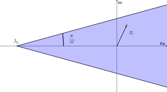
Figure 1: Illustration of $\mathcal{C}(\lambda_{i})$ in the complex plane.

To see this, we plot $\mathcal{C}(\lambda_{i})$ as the shaded area in Fig. 1. It is clear from the figure that

$$z_{i}\in\mathcal{C}(\lambda_{i})\;\Leftrightarrow\;|{\mathrm{Im}}(z_{i})|\leq\big{(}-\lambda_{i}+{\mathrm{Re}}(z_{i})\big{)}\tan\left(\frac{\pi}{M}\right),$$

which leads to

$$z_{i}\in\mathcal{C}(\lambda_{i})\;\Leftrightarrow\;\lambda_{i}\leq{\mathrm{Re}}(z_{i})-|{\mathrm{Im}}(z_{i})|\cot\left(\frac{\pi}{M}\right).$$

This, together with Eq. 18, gives the necessary and sufficient condition for Eq. ESDR-${\mathbf{X}}$ to be tight and we formally state it in Theorem 3.2.

Theorem 3.2.

Suppose that $M\geq 4$. Then Eq. ESDR-${\mathbf{X}}$ is tight if and only if

(19) $${\mathbf{Q}}+{\mathrm{Diag}}\big{(}\mathrm{Re}({\bm{z}})\big{)}-\cot\left(\frac{\pi}{M}\right){\mathrm{Diag}}(|\mathrm{Im}({\bm{z}})|\big{)}\succeq 0,$$

where ${\bm{z}}=[z_{1},z_{2},\ldots,z_{n}]^{\mathsf{T}}\in\mathbb{C}^{n}$.

Note that Eq. 19 is exactly the same as Eq. 5 if we recall the definitions of ${\mathbf{Q}}$ in Eq. 7 and $z_{i}$ in Eq. 17. Furthermore, if we set $M=2$ and ${\mathbf{H}},\;{\bm{v}}$ to be real in Eq. 5, it becomes the same as the previous result Eq. 10. Hence, our result extends Eq. 10 to the more general case where $M\geq 4$ and ${\mathbf{H}},\;{\bm{v}}$ are complex. Finally, the sufficient condition Eq. 4 in [17] can be derived from our result. Since

$$\mathrm{Re}(z_{i})-|{\mathrm{Im}}(z_{i})|\cot\left(\frac{\pi}{M}\right) =\frac{1}{\sin\left(\frac{\pi}{M}\right)}\left(\mathrm{Re}(z_{i})\sin\left(\frac{\pi}{M}\right)-|{\mathrm{Im}}(z_{i})|\cos\left(\frac{\pi}{M}\right)\right)$$

$$\geq-\frac{1}{\sin\left(\frac{\pi}{M}\right)}|z_{i}|\geq-\frac{1}{\sin\left(\frac{\pi}{M}\right)}\|{\mathbf{H}}^{\dagger}{\bm{v}}\|_{\infty},$$

we have

$${\mathrm{Diag}}\big{(}\mathrm{Re}({\bm{z}})\big{)}-\cot\left(\frac{\pi}{M}\right){\mathrm{Diag}}(|\mathrm{Im}({\bm{z}})|\big{)}\succeq-\frac{1}{\sin\left(\frac{\pi}{M}\right)}\|{\mathbf{H}}^{\dagger}{\bm{v}}\|_{\infty}{\mathbf{I}}_{n}.$$

Combining this with ${\mathbf{Q}}\succeq\lambda_{\mathrm{min}}({\mathbf{Q}}){\mathbf{I}}_{n}$, we can see that Eq. 4 is a stronger condition on ${\mathbf{H}}$ and ${\bm{v}}$ than Eq. 5.

3.2 Tightness of Eq. ESDR-${\mathbf{Y}}$

Similar to Theorem 3.1, we have the following characterization for Eq. ESDR-${\mathbf{Y}}$ to be tight. Since the proof technique is essentially the same as that in [17], we put the proof in a separate technical report [13].

Theorem 3.3.

Suppose that $M\geq 4$. Let the transmitted symbol vector ${\bm{x}}^{*}$ be

$$x_{i}^{*}=s_{u_{i}},\;u_{i}\in\{1,2,\ldots,M\},\;i=1,2,\ldots,n,$$

and define

(20) $$\hat{{\bm{v}}} =\begin{bmatrix}\mathrm{Re}({\bm{v}})\\ \mathrm{Im}({\bm{v}})\end{bmatrix}\in\mathbb{R}^{2n},\;\hat{{\mathbf{H}}}=\begin{bmatrix}\mathrm{Re}({\mathbf{H}})&-\mathrm{Im}({\mathbf{H}})\\ \mathrm{Im}({\mathbf{H}})&\mathrm{Re}({\mathbf{H}})\end{bmatrix}\in\mathbb{R}^{2n\times 2n},$$

$${\bm{y}}^{*} =\begin{bmatrix}\mathrm{Re}({\bm{x}}^{*})\\ \mathrm{Im}({\bm{x}}^{*})\end{bmatrix}\in\mathbb{R}^{2n},\;{\mathbf{Y}}^{*}={\bm{y}}^{*}({\bm{y}}^{*})^{\mathsf{T}}\in\mathbb{R}^{2n\times 2n}.$$

Then $({\bm{y}}^{*},{\mathbf{Y}}^{*})$ is the optimal solution of Eq. ESDR-${\mathbf{Y}}$ if and only if there exist ${{\bm{\lambda}}}\in\mathbb{R}^{2n}$, ${{\bm{\mu}}}\in\mathbb{R}^{n}$, and ${{\bm{g}}}\in\mathbb{R}^{2n}$ that satisfy

(21) $$\hat{{\mathbf{H}}}^{\mathsf{T}}\hat{{\bm{v}}}={{\bm{g}}}+({{\mathbf{\Lambda}}}+{{\mathbf{M}}}){\bm{y}}^{*},$$

(22) $$\langle{{\mathbf{\Gamma}}}_{i},{\mathbf{K}}_{u_{i}}\rangle\geq\langle{{\mathbf{\Gamma}}}_{i},{\mathbf{K}}_{j}\rangle,\;j=1,2,\ldots,M,\;i=1,2,\ldots,n,$$

and

$$\hat{{\mathbf{Q}}}+{{\mathbf{\Lambda}}}+{{\mathbf{M}}}\succeq 0,$$

where ${\mathbf{K}}_{j}$ is defined in Eq. 12, $\hat{{\mathbf{Q}}}$ is defined in Eq. 11, and

(23) $${{\mathbf{\Lambda}}}={\mathrm{Diag}}({{\bm{\lambda}}}),\;{{\mathbf{M}}}=\begin{bmatrix}\bm{0}&{\mathrm{Diag}}({{\bm{\mu}}})\\ {\mathrm{Diag}}({{\bm{\mu}}})&\bm{0}\end{bmatrix},\;{{\mathbf{\Gamma}}}_{i}=\begin{bmatrix}0&{g}_{i}&{g}_{n+i}\\ {g}_{i}&{\lambda}_{i}&{\mu}_{i}\\ {g}_{n+i}&{\mu}_{i}&{\lambda}_{n+i}\end{bmatrix}.$$

Furthermore, Eqs. 21 and 22 in Theorem 3.3 can be simplified to the following inequalities on $({\bm{\lambda}},{\bm{\mu}})$ (see Appendix A):

(24) $$\sin^{2}\biggl{(} \theta_{u_{i}}+\frac{\Delta\theta_{j}}{2}\biggr{)}\lambda_{i}+\cos^{2}\left(\theta_{u_{i}}+\frac{\Delta\theta_{j}}{2}\right)\lambda_{n+i}-\sin\left(2\theta_{u_{i}}+\Delta\theta_{j}\right)\mu_{j}$$

$$\leq{\mathrm{Re}}(z_{i})-\cot\left(\frac{\Delta\theta_{j}}{2}\right){\mathrm{Im}}(z_{i}),\;j\in\{1,2,\ldots,M\}\backslash\{u_{i}\},\;i=1,2,\ldots,n.$$

Here $\Delta\theta_{j}=\theta_{j}-\theta_{u_{i}}$, $\theta_{u_{i}}$ is the phase of the $i$-th transmitted symbol $x_{i}^{*}$, and $z_{i}$ is defined in Eq. 17. Similar to Eq. 18, we formulate the conditions in Theorem 3.3 as a semidefinite feasibility problem as follows:

(25) $$\mathrm{find} {\bm{\lambda}}\in\mathbb{R}^{2n}\;\text{and}\;{\bm{\mu}}\in\mathbb{R}^{n}$$

$$\mathrm{s.t.} \hat{{\mathbf{Q}}}+{\mathbf{\Lambda}}+{\mathbf{M}}\succeq 0,$$

Eq. 24 is satisfied,

where ${\mathbf{\Lambda}}$ and ${\mathbf{M}}$ are defined in Eq. 23. However, unlike problem Eq. 18 where every inequality only involves one dual variable, problem Eq. 25 has inequalities with three variables coupled together and it is unclear how to choose the “optimal” ${\bm{\lambda}}$ and ${\bm{\mu}}$. In the following, we give a simple necessary condition for Eq. ESDR-${\mathbf{Y}}$ being tight based on Eq. 25.

Theorem 3.4.

Suppose that $M\geq 4$. If Eq. ESDR-${\mathbf{Y}}$ is tight, then

(26) $${\mathbf{Q}}+{\mathrm{Diag}}\big{(}\mathrm{Re}({\bm{z}})\big{)}-\cot\left(\frac{2\pi}{M}\right){\mathrm{Diag}}(|\mathrm{Im}({\bm{z}})|\big{)}\succeq 0,$$

where ${\mathbf{Q}}={\mathbf{H}}^{\dagger}{\mathbf{H}}$ and ${\bm{z}}$ is defined in Eq. 17.

Before proving Theorem 3.4, we first introduce the following lemma.

Lemma 3.5.

Suppose that ${\mathbf{V}}$ is a PSD matrix in $\mathbb{R}^{2n}$ and is partitioned as

$${\mathbf{V}}=\begin{bmatrix}{\mathbf{A}}&{\mathbf{B}}\\ {\mathbf{B}}^{\mathsf{T}}&{\mathbf{C}}\end{bmatrix},$$

where ${\mathbf{A}}={\mathbf{A}}^{\mathsf{T}}$, ${\mathbf{C}}={\mathbf{C}}^{\mathsf{T}}$, and ${\mathbf{A}},{\mathbf{B}},{\mathbf{C}}\in\mathbb{R}^{n\times n}$. Then

$${\mathbf{U}}=\frac{1}{2}({\mathbf{A}}+{\mathbf{C}})+\frac{{\mathbf{i}}}{2}({\mathbf{B}}^{\mathsf{T}}-{\mathbf{B}})$$

is a PSD matrix in $\mathbb{C}^{n}$.

Proof 3.6.

We observe that

$${\mathbf{U}}=\frac{1}{2}\begin{bmatrix}{\mathbf{I}}_{n}&{\mathbf{i}}{\mathbf{I}}_{n}\end{bmatrix}\begin{bmatrix}{\mathbf{A}}&{\mathbf{B}}\\ {\mathbf{B}}^{\mathsf{T}}&{\mathbf{C}}\end{bmatrix}\begin{bmatrix}{\mathbf{I}}_{n}\\ -{\mathbf{i}}{\mathbf{I}}_{n}\end{bmatrix}.$$

The result follows immediately.

Proof 3.7 (Proof of Theorem 3.4).

If Eq. ESDR-${\mathbf{Y}}$ is tight, we can find ${{\bm{\lambda}}}\in\mathbb{R}^{2n}$ and ${{\bm{\mu}}}\in\mathbb{R}^{n}$ that satisfy the constraints in Eq. 25. By Lemma 3.5, the constraint $\hat{{\mathbf{Q}}}+{\mathbf{\Lambda}}+{\mathbf{M}}\succeq 0$ implies

(27) $${\mathbf{Q}}+{\mathrm{Diag}}({\bar{{\bm{\lambda}}}})\succeq 0,$$

where ${\bar{{\bm{\lambda}}}}\in\mathbb{R}^{n}$ is given by

$${\bar{\lambda}}_{i}=\frac{1}{2}(\lambda_{i}+\lambda_{n+i}),\;i=1,2,\ldots,n.$$

Fix $i\in\{1,2,\ldots,n\}$ and let $\hat{z}_{i}$ and $\hat{z}_{n+i}$ denote ${\mathrm{Re}}(z_{i})$ and ${\mathrm{Im}}(z_{i})$, respectively. If $\hat{z}_{n+i}\geq 0$, we set $\Delta\theta_{j}=\frac{2\pi}{M}$ in Eq. 24 to get

$$\sin^{2}\Bigl{(}\theta_{u_{i}}+\frac{\pi}{M}\Bigr{)}\lambda_{i}+\cos^{2}\Bigl{(}\theta_{u_{i}}+\frac{\pi}{M}\Bigr{)}\lambda_{n+i}-\sin\Bigl{(}2\theta_{u_{i}}+\frac{2\pi}{M}\Bigr{)}\mu_{j}\leq\hat{z}_{i}-\cot\Bigl{(}\frac{\pi}{M}\Bigr{)}|\hat{z}_{n+i}|.$$

Since $M\geq 4$, we can also set $\Delta\theta_{j}=\frac{2\pi}{M}+\pi$ to get

$$\cos^{2}\Bigl{(}\theta_{u_{i}}+\frac{\pi}{M}\Bigr{)}\lambda_{i}+\sin^{2}\Bigl{(}\theta_{u_{i}}+\frac{\pi}{M}\Bigr{)}\lambda_{n+i}+\sin\Bigl{(}2\theta_{u_{i}}+\frac{2\pi}{M}\Bigr{)}\mu_{j}\leq\hat{z}_{i}+\tan\Bigl{(}\frac{\pi}{M}\Bigr{)}|\hat{z}_{n+i}|.$$

Adding the above two inequalities and dividing both sides by two, we have

(28) $${\bar{\lambda}}_{i}=\frac{1}{2}(\lambda_{i}+\lambda_{n+i})\leq\hat{z}_{i}-\cot\left(\frac{2\pi}{M}\right)|\hat{z}_{n+i}|.$$

If $\hat{z}_{n+i}<0$, we can also arrive at Eq. 28 by setting $\Delta\theta_{j}$ to be $-\frac{2\pi}{M}$ and $-\frac{2\pi}{M}+\pi$, respectively. Finally, Theorem 3.4 follows from Eq. 27 and Eq. 28.

Note that Eq. 26 is the same as Eq. 6 if we recall the definitions of ${\mathbf{Q}}$ in Eq. 7 and $z_{i}$ in Eq. 17. Moreover, since Eq. ESDR-${\mathbf{Y}}$ is tighter than Eq. ESDR-${\mathbf{X}}$, Eq. ESDR-${\mathbf{Y}}$ will also be tight if Eq. 5 holds. Therefore, we have both a necessary condition Eq. 6 and a sufficient condition Eq. 5 for Eq. ESDR-${\mathbf{Y}}$ to be tight.

3.3 Tightness of Eq. ESDR1-${\mathbf{T}}$

In the same spirit, we first give a necessary and sufficient condition for Eq. ESDR1-${\mathbf{T}}$ to be tight. Since the technique is essentially the same as that used in Theorem 3.3, we omit the proof details due to the space limitation.

Theorem 3.8.

Suppose that $M\geq 4$. Let the transmitted symbol vector ${\bm{x}}^{*}$ be

$$x_{i}^{*}=s_{u_{i}},\;u_{i}\in\{1,2,\ldots,M\},\;i=1,2,\ldots,n,$$

and define

$${\bm{t}}^{*}_{i,u_{i}}=1,\;{\bm{t}}^{*}_{i,j}=0,\;j\neq u_{i},\;i=1,2,\ldots,n,$$

$${\mathbf{T}}^{*}={\bm{t}}^{*}({\bm{t}}^{*})^{\mathsf{T}}.$$

Then $({\bm{t}}^{*},{\mathbf{T}}^{*})$ is the optimal solution of (ESDR1-${\mathbf{T}}$) if and only if there exist ${{\bm{\alpha}}}\in\mathbb{R}^{n}$ and ${{{\bm{\gamma}}}}\in\mathbb{R}^{Mn}$ such that

(29) $${\mathrm{Diag}}(1-2{\bm{t}}^{*}){{\bm{\gamma}}}=-2{\hat{{\mathbf{S}}}}^{\mathsf{T}}\hat{{\mathbf{H}}}^{\mathsf{T}}\hat{{\bm{v}}}+{{\bm{\alpha}}}\otimes{\bm{1}}_{M},$$

and

(30) $$\bar{{\mathbf{Q}}}+{\mathrm{Diag}}({{{{\bm{\gamma}}}}})\succeq 0.$$

where $\hat{{\mathbf{S}}}$ is defined in Eq. 14, $\hat{{\mathbf{H}}},\;\hat{{\bm{v}}}$ are defined in Eq. 20, and $\bar{{\mathbf{Q}}}$ is defined in Eq. 16.

Now we provide a corollary that will serve as our basis for further derivation.

Corollary 3.9.

If (ESDR1-${\mathbf{T}}$) is tight, then there exist

$${{\bm{\alpha}}}\in\mathbb{R}^{n}\;\text{and}\;{{\bm{\gamma}}}_{1},{{\bm{\gamma}}}_{2},\ldots,{{\bm{\gamma}}}_{n}\in\mathbb{R}^{M}$$

that satisfy

(31) $${\gamma}_{i,j}=\begin{cases}-2\mathrm{Re}[s_{j}^{\dagger}({\mathbf{H}}^{\dagger}{\bm{v}})_{i}]+{\alpha}_{i},\;\;\;&\text{if}\;j\neq u_{i},\\ 2\mathrm{Re}[s_{j}^{\dagger}({\mathbf{H}}^{\dagger}{\bm{v}})_{i}]-{\alpha}_{i},\;\;\;&\text{if}\;j=u_{i},\end{cases}\;j=1,2,\ldots,M,\;i=1,2,\ldots,n,$$

and

$${\bm{w}}^{\mathsf{T}}{\mathrm{Diag}}({{\bm{\gamma}}_{i}}){\bm{w}}\geq 0,\;\;i=1,2,\ldots,n,$$

for any ${\bm{w}}\in\mathbb{R}^{M}$ such that ${\bm{w}}^{\mathsf{T}}{\bm{s}}_{R}={\bm{w}}^{\mathsf{T}}{\bm{s}}_{I}=0$.

Proof 3.10.

By Theorem 3.8, if Eq. ESDR1-${\mathbf{T}}$ is tight, we can find ${{\bm{\alpha}}}\in\mathbb{R}^{n}$ and ${{\bm{\gamma}}}\in\mathbb{R}^{Mn}$ that satisfy (29) and (30). Let ${\bm{\gamma}}$ be partitioned as ${{\bm{\gamma}}}=[{{\bm{\gamma}}}_{1}^{\mathsf{T}},{{\bm{\gamma}}}_{2}^{\mathsf{T}},\ldots,{{\bm{\gamma}}}_{n}^{\mathsf{T}}]^{\mathsf{T}}$ where ${{\bm{\gamma}}}_{j}\in\mathbb{R}^{M}$ is the $j$-th block of ${{\bm{\gamma}}}$. It is straightforward to verify that (29) is equivalent to (31).

Moreover, for any $i\in\{1,2,\ldots,n\}$ and any ${\bm{w}}\in\mathbb{R}^{M}$ that satisfies ${\bm{w}}^{\mathsf{T}}{\bm{s}}_{R}={\bm{w}}^{\mathsf{T}}{\bm{s}}_{I}=0$, we set $\bar{{\bm{w}}}=[\bar{{\bm{w}}}_{1}^{\mathsf{T}},\bar{{\bm{w}}}_{2}^{\mathsf{T}},\ldots,\bar{{\bm{w}}}_{n}^{\mathsf{T}}]^{\mathsf{T}}\in\mathbb{R}^{Mn}$ to be

$$\bar{{\bm{w}}}_{j}=\begin{cases}{\bm{0}},&\text{if}\;j\neq i,\\ {\bm{w}},&\text{if}\;j=i.\end{cases}$$

It is simple to check that $\hat{{{\mathbf{S}}}}\bar{{\bm{w}}}={\bm{0}}$. Therefore, recalling that $\bar{{\mathbf{Q}}}=\hat{{{\mathbf{S}}}}^{\mathsf{T}}{\hat{\mathbf{Q}}}\hat{{{\mathbf{S}}}}$, by (30) we have

$$\bar{{\bm{w}}}^{\mathsf{T}}(\bar{{\mathbf{Q}}}+{\mathrm{Diag}}({{{{\bm{\gamma}}}}}))\bar{{\bm{w}}}=\bar{{\bm{w}}}^{\mathsf{T}}{\mathrm{Diag}}({{{{\bm{\gamma}}}}})\bar{{\bm{w}}}={\bm{w}}^{\mathsf{T}}{\mathrm{Diag}}({{\bm{\gamma}}_{i}}){\bm{w}}\geq 0.$$

The proof is complete.

In practice, the symbol set ${\mathcal{S}}$, such as the one in Eq. 3 considered in this paper, is symmetric with respect to the origin. Therefore, we can find $u_{i}^{\prime}\in\{1,2,\ldots,M\}$ that satisfies $s_{u_{i}^{\prime}}=-s_{u_{i}}$. Now let ${\bm{w}}\in\mathbb{R}^{M}$ be

$$w_{j}=\begin{cases}0,&\text{if}\;j\notin\{u_{i},u_{i}^{\prime}\},\\ 1,&\text{if}\;j\in\{u_{i},u_{i}^{\prime}\},\end{cases}\;j=1,2,\ldots,M.$$

We have ${\bm{w}}^{\mathsf{T}}{\bm{s}}_{R}=s_{R,u_{i}}+s_{R,u_{i}^{\prime}}=0$ and ${\bm{w}}^{\mathsf{T}}{\bm{s}}_{I}=s_{I,u_{i}}+s_{I,u_{i}^{\prime}}=0$. Hence, when Eq. ESDR1-${\mathbf{T}}$ is tight, Corollary 3.9 implies that

$${\bm{w}}^{\mathsf{T}}{\mathrm{Diag}}({{\bm{\gamma}}_{i}}){\bm{w}}={\gamma}_{u_{i}}+{\gamma}_{u_{i}^{\prime}}=4\mathrm{Re}[s_{u_{i}}^{\dagger}({\mathbf{H}}^{\dagger}{\bm{v}})_{i}]=4\mathrm{Re}[(x_{i}^{*})^{\dagger}({\mathbf{H}}^{\dagger}{\bm{v}})_{i}]\geq 0.$$

This immediately leads to the following upper bound on the tightness probability of Eq. ESDR1-${\mathbf{T}}$.

Corollary 3.11.

Suppose that the symbol set ${\mathcal{S}}$ is symmetric with respect to the origin and $0\notin{\mathcal{S}}$. We further assume that

1. The entries of ${\bm{x}}^{*}$ are drawn from ${\mathcal{S}}$ uniformly and independently;

2. ${\bm{x}}^{*}$, ${\mathbf{H}}$, and ${\bm{v}}$ are mutually independent; and

3. the distribution of ${\mathbf{H}}$ and ${\bm{v}}$ are continuous.

Then we have

$$\mathbf{Prob}\bigl{(}\text{\lx@cref{creftype~refnum}{eq:Model II} is tight}\bigr{)}\leq\left(\frac{1}{2}\right)^{n}.$$

Proof 3.12.

Let $z_{i}=(x_{i}^{*})^{\dagger}({\mathbf{H}}^{\dagger}{\bm{v}})_{i}$, $i=1,2,\ldots,n$. Since ${\mathbf{H}}$ and ${\bm{v}}$ are independent continuous random variables, the event

$$\bigcup_{i=1}^{n}\bigcup_{s\in{\mathcal{S}}}\{\mathrm{Re}(s^{\dagger}({\mathbf{H}}^{\dagger}{\bm{v}})_{i})=0\}$$

happens with probability zero. Hence, because of the symmetry of ${\mathcal{S}}$, with probability one exactly half of the symbols $s\in{\mathcal{S}}$ satisfy $\mathrm{Re}(s^{\dagger}({\mathbf{H}}^{\dagger}{\bm{v}})_{i})>0$ for each $i\in\{1,2,\ldots,n\}$ when ${\mathbf{H}}$ and ${\bm{v}}$ are given. By the assumption that $x^{*}_{i}$ is uniformly distributed over ${\mathcal{S}}$, we obtain

$$\mathbf{Prob}\bigl{(}\mathrm{Re}(z_{i})\geq 0{\>|\>}{\mathbf{H}},{\bm{v}}\bigr{)}=\frac{1}{2}\;\text{almost surely}.$$

Moreover, $\{z_{i}\}_{i=1}^{n}$ are mutually independent conditioned on ${\mathbf{H}}$ and ${\bm{v}}$. This leads to

$$\mathbf{Prob}\bigl{(}\mathrm{Re}(z_{i})\geq 0,\;i=1,2,\ldots,n\bigr{)} =\operatorname*{\mathbb{E}}_{{\mathbf{H}},{\bm{v}}}\bigl{[}\mathbf{Prob}\bigl{(}\mathrm{Re}(z_{i})\geq 0,\;i=1,2,\ldots,n{\>|\>}{\mathbf{H}},{\bm{v}}\bigr{)}\bigr{]}$$

$$=\operatorname*{\mathbb{E}}_{{\mathbf{H}},{\bm{v}}}\bigl{[}\prod_{i=1}^{n}\mathbf{Prob}\bigl{(}\mathrm{Re}(z_{i})\geq 0{\>|\>}{\mathbf{H}},{\bm{v}}\bigr{)}\bigr{]}$$

$$=\left(\frac{1}{2}\right)^{n}.$$

Finally, Corollary 3.11 follows from the fact that the tightness of Eq. ESDR1-${\mathbf{T}}$ implies ${\mathrm{Re}}(z_{i})\geq 0$, $i=1,2,\ldots,n$.

It is worth noting that all the assumptions in Corollary 3.11 are mild: they are satisfied if we use the $M$-PSK or QAM modulation scheme and the entries of ${\mathbf{H}}$ and ${\bm{v}}$ follow the complex Gaussian distribution.

Intuitively, we will expect that Eq. ESDR1-${\mathbf{T}}$ is less likely to recover the transmitted symbols with an increasing symbol set size $M$. In the following, we present a more refined upper bound on the tightness probability specific to the $M$-PSK setting and the proof can be found in [13].

Theorem 3.13.

Suppose that $M$-PSK is used with $M\geq 4$ and the same assumptions in Corollary 3.11 hold. Then we have

$$\mathbf{Prob}\bigl{(}\text{\lx@cref{creftype~refnum}{eq:Model II} is tight}\bigr{)}\leq\left(\frac{2}{M}\right)^{n}.$$

From Corollaries 3.11 and 3.13, we can see that the tightness probability of Eq. ESDR1-${\mathbf{T}}$ is bounded away from one regardless of the noise level, and it tends to zero exponentially fast when the number of transmitted symbols $n$ increases. This is in sharp contrast to Eqs. ESDR-${\mathbf{X}}$ and ESDR-${\mathbf{Y}}$, whose tightness probabilities will approach one if the noise level is sufficiently small and the number of received signals $m$ is sufficiently large compared to $n$ [17, Theorem 4.5].

4 Equivalence between different SDRs

In this section, we focus on the relationship between different SDR models of Eq. 2.Related to the SDRs discussed so far, a recent paper [16] proved that Eq. ESDR2-${\mathbf{T}}$ is equivalent to Eq. ESDR-${\mathbf{Y}}$ for the MIMO detection problem with a general symbol set. An earlier paper [21] compared three different SDRs in the QAM setting and showed their equivalence. Compared with those in Section 2, the SDRs considered in [21] differ greatly in their motivations and structures, and the two equivalence results are proved using different techniques. In this section, we provide a more general equivalence theorem from which both results follow as special cases. This not only reveals the underlying connection between these two works, but also may potentially lead to new equivalence between SDRs.

4.1 Review of previous results

In [16], the authors established the following correspondence between a pair of feasible points of Eq. ESDR2-${\mathbf{T}}$ and Eq. ESDR-${\mathbf{Y}}$:

(32) $${\mathbf{Y}}=\hat{{\mathbf{S}}}{\mathbf{T}}\hat{{\mathbf{S}}}^{\mathsf{T}}\;\text{and}\;{\bm{y}}=\hat{{\mathbf{S}}}{\bm{t}},$$

where $\hat{{\mathbf{S}}}\in\mathbb{R}^{2n\times Mn}$ is defined in Eq. 14. In [21], the authors considered the feasible set of a virtually-antipodal SDR (VA-SDR):

(VA-SDR) $$\begin{bmatrix}1&{\bm{b}}^{\mathsf{T}}\\ {\bm{b}}&{\mathbf{B}}\end{bmatrix}\in\mathbb{S}_{+}^{qn+1}$$

$$\mathrm{s.t.} B_{i,i}=1,\;i=1,2,\ldots,qn,$$

and that of a bounded-constrained SDR (BC-SDR):

(BC-SDR) $$\begin{bmatrix}1&{\bm{x}}^{\mathsf{T}}\\ {\bm{x}}&{\mathbf{X}}\end{bmatrix}\in\mathbb{S}_{+}^{n+1}$$

$$\mathrm{s.t.} 1\leq X_{i,i}\leq(2^{q}-1)^{2},\;i=1,2,\ldots,n,$$

where $q\geq 1$ is an integer. We refer interested readers to [21] and references therein for their derivations. The authors proved the equivalence between Eq. VA-SDR and Eq. BC-SDR by showing the following correspondence:

(33) $${\mathbf{X}}={{\mathbf{W}}}{\mathbf{B}}{{\mathbf{W}}}^{\mathsf{T}}\;\text{and}\;{\bm{x}}={{\mathbf{W}}}{\bm{b}},$$

where

$${\mathbf{W}}=\begin{bmatrix}{\mathbf{I}}_{n}&2{\mathbf{I}}_{n}&4{\mathbf{I}}_{n}&\ldots&2^{q-1}{\mathbf{I}}_{n}\end{bmatrix}\in\mathbb{R}^{n\times qn}.$$

Note that both equivalence results in (32) and (33) fall into the following form:

$$\left\{\begin{bmatrix}1&{\bm{y}}^{\mathsf{T}}\\ {\bm{y}}&{\mathbf{Y}}\end{bmatrix}\in\mathcal{F}_{1}\right\}=\left\{\begin{bmatrix}1&{\bm{y}}^{\mathsf{T}}\\ {\bm{y}}&{\mathbf{Y}}\end{bmatrix}=\begin{bmatrix}1&{\bm{0}}\\ {\bm{0}}&{\mathbf{P}}\end{bmatrix}\begin{bmatrix}1&{\bm{t}}^{\mathsf{T}}\\ {\bm{t}}&{\mathbf{T}}\end{bmatrix}\begin{bmatrix}1&{\bm{0}}\\ {\bm{0}}&{\mathbf{P}}^{\mathsf{T}}\end{bmatrix}:\;\begin{bmatrix}1&{\bm{t}}^{\mathsf{T}}\\ {\bm{t}}&{\mathbf{T}}\end{bmatrix}\in\mathcal{F}_{2}\right\},$$

where $\mathcal{F}_{1}$ is a subset of $\mathbb{S}_{+}^{k+1}$, $\mathcal{F}_{2}$ is a subset of $\mathbb{S}_{+}^{d+1}$, and we call ${\mathbf{P}}\in\mathbb{R}^{k\times d}$ as the transformation matrix. Moreover, both the transformation matrices $\hat{{\mathbf{S}}}$ in (32) and ${\mathbf{W}}$ in (33) have a special “separable” property that we now define for ease of presentation.

Definition 4.1.

A matrix ${\mathbf{P}}\in\mathbb{R}^{k\times d}$ is called separable if there exist a partition of rows $\alpha_{1},\alpha_{2},\ldots,\alpha_{l}$ and a partition of columns $\beta_{1},\beta_{2},\ldots,\beta_{l}$ such that

$${\mathbf{P}}[\alpha_{i},\beta_{j}]=\mathbf{0},\qquad\forall\;i\neq j.$$

In other words, a matrix is separable if, after possibly rearranging rows and columns, it has a block diagonal structure. In particular, for the transformation matrix $\hat{{\mathbf{S}}}$ in Eq. 32, the corresponding row and column partitions are given by

(34) $$\alpha_{i}=\{i,n+i\},\;\beta_{i}=\{(i-1)M+1,(i-1)M+2,\ldots,iM\},\;i=1,2,\ldots,n;$$

for the transformation matrix ${\mathbf{W}}$ in Eq. 33, they are given by

(35) $$\alpha_{i}=\{i\},\;\beta_{i}=\{i,i+n,i+2n,\ldots,i+(q-1)n\},\;i=1,2,\ldots,n.$$

4.2 A general equivalence theorem

Now we are ready to present our main equivalence result.

Theorem 4.2.

Suppose that the matrix ${\mathbf{P}}\in\mathbb{R}^{k\times d}$ is separable with row partition $\alpha_{1},\alpha_{2},\ldots,\alpha_{l}$ and column partition $\beta_{1},\beta_{2},\ldots,\beta_{l}$.Moreover, define

$$k_{i}:=|\alpha_{i}|,\;d_{i}:=|\beta_{i}|,\;\text{and}\;{\mathbf{P}}_{i}:={\mathbf{P}}[\alpha_{i},\beta_{i}]\in\mathbb{R}^{k_{i}\times d_{i}},\;i=1,2,\ldots,l,$$

where we use $|\cdot|$ to denote the cardinality of a set. Then given arbitrary constraint sets ${\mathcal{A}_{i}\subset\mathbb{R}^{d_{i}\times d_{i}}}$ for $i=1,2,\ldots,l$, the following set

(36) $$\begin{bmatrix}1&{\bm{y}}^{\mathsf{T}}\\ {\bm{y}}&{\mathbf{Y}}\end{bmatrix}\in\mathbb{S}_{+}^{k+1}$$

$$\mathrm{s.t.} {\mathbf{Y}}={\mathbf{P}}{\mathbf{T}}{\mathbf{P}}^{\mathsf{T}},\;{\bm{y}}={\mathbf{P}}{\bm{t}},$$

$$\begin{bmatrix}1&{\bm{t}}^{\mathsf{T}}\\ {\bm{t}}&{\mathbf{T}}\end{bmatrix}\in\mathbb{S}_{+}^{d+1},$$

$$\begin{bmatrix}1&{\bm{t}}[\beta_{i}]^{\mathsf{T}}\\ {\bm{t}}[\beta_{i}]&{\mathbf{T}}[\beta_{i}]\end{bmatrix}\in\mathcal{A}_{i},\;i=1,2,\ldots,l,$$

where the variables are ${\bm{y}}\in\mathbb{R}^{k}$, ${\mathbf{Y}}\in\mathbb{R}^{k\times k}$, ${\bm{t}}\in\mathbb{R}^{d}$, and ${\mathbf{T}}\in\mathbb{R}^{d\times d}$, is the same as

(37) $$\begin{bmatrix}1&{\bm{y}}^{\mathsf{T}}\\ {\bm{y}}&{\mathbf{Y}}\end{bmatrix}\in\mathbb{S}_{+}^{k+1}$$

$$\mathrm{s.t.} {\mathbf{Y}}[\alpha_{i}]={\mathbf{P}}_{i}{\mathbf{T}}^{(i)}{\mathbf{P}}_{i}^{\mathsf{T}},\;{\bm{y}}[\alpha_{i}]={\mathbf{P}}_{i}{\bm{t}}^{(i)},$$

$$\begin{bmatrix}1&({\bm{t}}^{(i)})^{\mathsf{T}}\\ {\bm{t}}^{(i)}&{\mathbf{T}}^{(i)}\end{bmatrix}\in\mathbb{S}_{+}^{d_{i}+1},$$

$$\begin{bmatrix}1&({\bm{t}}^{(i)})^{\mathsf{T}}\\ {\bm{t}}^{(i)}&{\mathbf{T}}^{(i)}\end{bmatrix}\in\mathcal{A}_{i},\;i=1,2,\ldots,l,$$

where the variables are ${\bm{y}}\in\mathbb{R}^{k}$, ${\mathbf{Y}}\in\mathbb{R}^{k\times k}$, ${\bm{t}}^{(i)}\in\mathbb{R}^{d_{i}}$, and ${\mathbf{T}}^{(i)}\in\mathbb{R}^{d_{i}\times d_{i}}$ with $i=1,2,\ldots,l$.

The following lemma will be useful in our proof.

Lemma 4.3 ([8, Theorem 7.3.11]).

Let ${\mathbf{A}}\in\mathbb{R}^{p\times n}$ and ${\mathbf{B}}\in\mathbb{R}^{q\times n}$ where $p\leq q$. Then ${\mathbf{A}}^{\mathsf{T}}{\mathbf{A}}={\mathbf{B}}^{\mathsf{T}}{\mathbf{B}}$ if and only if there exists a matrix ${\mathbf{U}}\in\mathbb{R}^{q\times p}$ with ${\mathbf{U}}^{\mathsf{T}}{\mathbf{U}}={\mathbf{I}}_{p}$ such that ${\mathbf{B}}={\mathbf{U}}{\mathbf{A}}$.

Proof 4.4 (Proof of Theorem 4.2).

Without loss of generality, we assume the transformation matrix ${\mathbf{P}}\in\mathbb{R}^{k\times d}$ is in the form

$${\mathbf{P}}=\begin{bmatrix}{\mathbf{P}}_{1}&&&\\ &{\mathbf{P}}_{2}&&\\ &&\ddots&\\ &&&{\mathbf{P}}_{l}\end{bmatrix},$$

where ${\mathbf{P}}_{i}\in\mathbb{R}^{k_{i}\times d_{i}}$, $\sum_{i=1}^{l}k_{i}=k$, and $\sum_{i=1}^{l}d_{i}=d$.

For one direction, suppose that $({\bm{y}},{\mathbf{Y}},{\bm{t}},{\mathbf{T}})$ satisfies the constraints in Eq. 36. Then it is straightforward to see that $({\bm{y}},{\mathbf{Y}})$ also satisfies the constraints in Eq. 37 together with

$${\bm{t}}^{(i)}={\bm{t}}[\beta_{i}],\;{\mathbf{T}}^{(i)}={\mathbf{T}}[\beta_{i}],\;i=1,2,\ldots,l.$$

The other direction of the proof is more involved. Given $({\bm{y}},{\mathbf{Y}})$ and the variables $\{{\bm{t}}^{(i)},{\mathbf{T}}^{(i)}\}_{i=1}^{l}$ in Eq. 37, our goal is to construct $({\bm{t}},{\mathbf{T}})$ satisfying the conditions in Eq. 36. To simplify the notations, we define

(38) $$\tilde{{\mathbf{Y}}}:=\begin{bmatrix}1&{\bm{y}}^{\mathsf{T}}\\ {\bm{y}}&{\mathbf{Y}}\end{bmatrix},\;\tilde{{\mathbf{T}}}^{(i)}:=\begin{bmatrix}1&({\bm{t}}^{(i)})^{\mathsf{T}}\\ {\bm{t}}^{(i)}&{\mathbf{T}}^{(i)}\end{bmatrix},\;\text{and}\;\tilde{{\mathbf{P}}}_{i}:=\begin{bmatrix}1&{\bm{0}}\\ {\bm{0}}&{\mathbf{P}}_{i}\end{bmatrix}.$$

Let $r=\max\{k,d\}$. Since $\tilde{{\mathbf{Y}}}\in\mathbb{S}_{+}^{k+1}$, it can be factorized as

(39) $$\tilde{{\mathbf{Y}}}=\tilde{{\mathbf{V}}}^{\mathsf{T}}\tilde{{\mathbf{V}}},$$

where $\tilde{{\mathbf{V}}}\in\mathbb{R}^{(r+1)\times(k+1)}$. The above factorization can be done because $r\geq k$. Further, we partition $\tilde{{\mathbf{V}}}$ as

$$\tilde{{\mathbf{V}}}=\begin{bmatrix}{\bm{v}}&{\mathbf{V}}_{1}&{\mathbf{V}}_{2}&\ldots&{\mathbf{V}}_{l}\end{bmatrix},$$

where ${\bm{v}}\in\mathbb{R}^{r+1}$ and ${\mathbf{V}}_{i}\in\mathbb{R}^{(r+1)\times k_{i}}$ contains the columns of $\tilde{{\mathbf{V}}}$ indexed by $\alpha_{i}$ for $i=1,2,\ldots,l$. Moreover, we have ${\bm{v}}^{\mathsf{T}}{\bm{v}}=\tilde{{\mathbf{Y}}}_{1,1}=1$. Similarly, $\tilde{{\mathbf{T}}}^{(i)}$ can be factorized as

(40) $$\tilde{{\mathbf{T}}}^{(i)}=(\tilde{{\mathbf{Z}}}^{(i)})^{\mathsf{T}}\tilde{{\mathbf{Z}}}^{(i)},\;i=1,2,\ldots,l,$$

where $\tilde{{\mathbf{Z}}}^{(i)}\in\mathbb{R}^{(d_{i}+1)\times(d_{i}+1)}$ and is partitioned as

(41) $$\tilde{{\mathbf{Z}}}^{(i)}=\begin{bmatrix}{\bm{z}}^{(i)}&{\mathbf{Z}}^{(i)}\end{bmatrix}.$$

Combining Eq. 40 with the equality constraints in Eq. 37, we get

$$\begin{bmatrix}1&{\bm{y}}[\alpha_{i}]^{\mathsf{T}}\\ {\bm{y}}[\alpha_{i}]&{\mathbf{Y}}[\alpha_{i}]\end{bmatrix}=\tilde{{\mathbf{P}}}_{i}\tilde{{\mathbf{T}}}^{(i)}\tilde{{\mathbf{P}}}^{\mathsf{T}}_{i}=\bigl{(}\tilde{{\mathbf{Z}}}^{(i)}\tilde{{\mathbf{P}}}^{\mathsf{T}}_{i}\bigr{)}^{\mathsf{T}}\bigl{(}\tilde{{\mathbf{Z}}}^{(i)}\tilde{{\mathbf{P}}}^{\mathsf{T}}_{i}\bigr{)},\;i=1,2,\ldots,l,$$

where $\tilde{{\mathbf{Z}}}^{(i)}\tilde{{\mathbf{P}}}^{\mathsf{T}}_{i}\in\mathbb{R}^{(d_{i}+1)\times(k_{i}+1)}$. On the other hand, the factorization in Eq. 39 implies

$$\begin{bmatrix}1&{\bm{y}}[\alpha_{i}]^{\mathsf{T}}\\ {\bm{y}}[\alpha_{i}]&{\mathbf{Y}}[\alpha_{i}]\end{bmatrix}=\begin{bmatrix}{\bm{v}}&{\mathbf{V}}_{i}\end{bmatrix}^{\mathsf{T}}\begin{bmatrix}{\bm{v}}&{\mathbf{V}}_{i}\end{bmatrix},$$

where $[{\bm{v}}\quad{\mathbf{V}}_{i}]\in\mathbb{R}^{(r+1)\times(k_{i}+1)}$. By Lemma 4.3, we can find ${\mathbf{U}}_{i}\in\mathbb{R}^{(r+1)\times(d_{i}+1)}$ with ${\mathbf{U}}_{i}^{\mathsf{T}}{\mathbf{U}}_{i}={\mathbf{I}}_{d_{i}+1}$ such that

(42) $$\begin{bmatrix}{\bm{v}}&{\mathbf{V}}_{i}\end{bmatrix}={\mathbf{U}}_{i}\tilde{{\mathbf{Z}}}^{(i)}\tilde{{\mathbf{P}}}^{\mathsf{T}}_{i}.$$

Substituting Eq. 38 and Eq. 41 into Eq. 42, we get

(43) $${\bm{v}}={\mathbf{U}}_{i}{\bm{z}}^{(i)}\;\text{and}\;{\mathbf{V}}_{i}={\mathbf{U}}_{i}{{\mathbf{Z}}}^{(i)}{\mathbf{P}}_{i}^{\mathsf{T}}.$$

Finally, we define

$${\mathbf{R}}=\begin{bmatrix}{\bm{v}}&{\mathbf{U}}_{1}{{\mathbf{Z}}}^{(1)}&{\mathbf{U}}_{2}{{\mathbf{Z}}}^{(2)}&\ldots&{\mathbf{U}}_{l}{{\mathbf{Z}}}^{(l)}\end{bmatrix}\in\mathbb{R}^{(r+1)\times(d+1)},$$

whose columns indexed by $\beta_{i}$ are given by ${\mathbf{U}}_{i}{{\mathbf{Z}}}^{(i)}$, and construct $({\bm{t}},{\mathbf{T}})$ by

(44) $$\begin{bmatrix}1&{\bm{t}}^{\mathsf{T}}\\ {\bm{t}}&{\mathbf{T}}\end{bmatrix}={\mathbf{R}}^{\mathsf{T}}{\mathbf{R}}.$$

Next we verify that $({\bm{t}},{\mathbf{T}})$ in Eq. 44 indeed satisfies all the constraints in Eq. 36. The positive semidefiniteness is evident by our construction. For the equality constraints, by using Eq. 43 we have

$${\mathbf{R}}\begin{bmatrix}1&{\bm{0}}\\ {\bm{0}}&{\mathbf{P}}^{\mathsf{T}}\end{bmatrix} =\begin{bmatrix}{\bm{v}}&{\mathbf{U}}_{1}{{\mathbf{Z}}}^{(1)}{\mathbf{P}}_{1}^{\mathsf{T}}&{\mathbf{U}}_{1}{{\mathbf{Z}}}^{(2)}{\mathbf{P}}_{2}^{\mathsf{T}}&\ldots&{\mathbf{U}}_{l}{{\mathbf{Z}}}^{(l)}{\mathbf{P}}_{l}^{\mathsf{T}}\end{bmatrix}$$

$$=\begin{bmatrix}{\bm{v}}&{\mathbf{V}}_{1}&{\mathbf{V}}_{2}&\ldots&{\mathbf{V}}_{l}\end{bmatrix}$$

$$=\tilde{{\mathbf{V}}}.$$

Hence, we get

$$\begin{bmatrix}1&{\bm{0}}\\ {\bm{0}}&{\mathbf{P}}\end{bmatrix}\begin{bmatrix}1&{\bm{t}}^{\mathsf{T}}\\ {\bm{t}}&{\mathbf{T}}\end{bmatrix}\begin{bmatrix}1&{\bm{0}}\\ {\bm{0}}&{\mathbf{P}}^{\mathsf{T}}\end{bmatrix} =\begin{bmatrix}1&{\bm{0}}\\ {\bm{0}}&{\mathbf{P}}\end{bmatrix}{\mathbf{R}}^{\mathsf{T}}{\mathbf{R}}\begin{bmatrix}1&{\bm{0}}\\ {\bm{0}}&{\mathbf{P}}^{\mathsf{T}}\end{bmatrix}$$

$$=\tilde{{\mathbf{V}}}^{\mathsf{T}}\tilde{{\mathbf{V}}}$$

$$=\begin{bmatrix}1&{\bm{y}}^{\mathsf{T}}\\ {\bm{y}}&{\mathbf{Y}}\end{bmatrix},$$

which is equivalent to ${\mathbf{Y}}={\mathbf{P}}{\mathbf{T}}{\mathbf{P}}^{\mathsf{T}}$ and ${\bm{y}}={\mathbf{P}}{\bm{t}}$. Lastly, note that

(45) $$\begin{bmatrix}1&{\bm{t}}[\beta_{i}]^{\mathsf{T}}\\ {\bm{t}}[\beta_{i}]&{\mathbf{T}}[\beta_{i}]\end{bmatrix} =\begin{bmatrix}{\bm{v}}&{\mathbf{U}}_{i}{\mathbf{Z}}^{(i)}\end{bmatrix}^{\mathsf{T}}\begin{bmatrix}{\bm{v}}&{\mathbf{U}}_{i}{\mathbf{Z}}^{(i)}\end{bmatrix}$$

(46) $$=\begin{bmatrix}{\mathbf{U}}_{i}{\bm{z}}^{(i)}&{\mathbf{U}}_{i}{\mathbf{Z}}^{(i)}\end{bmatrix}^{\mathsf{T}}\begin{bmatrix}{\mathbf{U}}_{i}{\bm{z}}^{(i)}&{\mathbf{U}}_{i}{\mathbf{Z}}^{(i)}\end{bmatrix}$$

$$=(\tilde{{\mathbf{Z}}}^{(i)})^{\mathsf{T}}{\mathbf{U}}_{i}^{\mathsf{T}}{\mathbf{U}}_{i}\tilde{{\mathbf{Z}}}^{(i)}$$

(47) $$=(\tilde{{\mathbf{Z}}}^{(i)})^{\mathsf{T}}\tilde{{\mathbf{Z}}}^{(i)}$$

$$=\tilde{{\mathbf{T}}}^{(i)}=\begin{bmatrix}1&({\bm{t}}^{(i)})^{\mathsf{T}}\\ {\bm{t}}^{(i)}&{\mathbf{T}}^{(i)}\end{bmatrix},$$

where we used Eq. 44 in Eq. 45, ${\bm{v}}={\mathbf{U}}_{i}{\bm{z}}^{(i)}$ (cf. Eq. 43) in Eq. 46, and ${\mathbf{U}}_{i}^{\mathsf{T}}{\mathbf{U}}_{i}={\mathbf{I}}_{d_{i}+1}$ in Eq. 47. Hence, the remaining constraints in Eq. 36 are also satisfied because of the conditions on $\tilde{{\mathbf{T}}}^{(i)}$ in Eq. 37.

The proof of Theorem 4.2 is complete.

Two remarks are in order. Firstly, the variables in Eq. 36 are in a high-dimensional PSD cone $\mathbb{S}_{+}^{d+1}$, while those in Eq. 37 are in the Cartesian product of smaller PSD cones $\mathbb{S}_{+}^{k+1}\times\mathbb{S}_{+}^{d_{1}+1}\times\mathbb{S}_{+}^{d_{2}+1}\times\cdots\times\mathbb{S}_{+}^{d_{l}+1}$. When $k,\;d_{1},\;d_{2},\ldots,d_{l}$ are much smaller than $d$, using Eq. 37 instead of Eq. 36 can achieve dimension reduction without any additional cost. This can bring substantially higher computational efficiency for solving the corresponding SDP in practice (see Section 5). Secondly, Theorem 4.2 is very general and thus could be applicable to a potentially wide range of problems. It is worth highlighting that we require no assumptions on the sets $\mathcal{A}_{i}$ that constrain the submatrices, as well as the row and column partitions of the separable matrix ${\mathbf{P}}$. This enables us to accommodate both the equivalence results Eq. 32 and Eq. 33, as we will show next.

4.2.1 Equivalence between Eq. ESDR2-${\mathbf{T}}$ and Eq. ESDR-${\mathbf{Y}}$

As we noted before, the transformation matrix $\hat{{\mathbf{S}}}$ in Eq. 32 is separable with the row and column partitions given in Eq. 34 and we have

$$\hat{{\mathbf{S}}}[\alpha_{i},\beta_{i}]=\begin{bmatrix}{\bm{s}}^{\mathsf{T}}_{R}\\ {\bm{s}}^{\mathsf{T}}_{I}\end{bmatrix}\in\mathbb{R}^{2\times M},\;i=1,2,\ldots,n.$$

Moreover, we can see that the feasible set of Eq. ESDR2-${\mathbf{T}}$ is in the form of Eq. 36 with the set $\mathcal{A}_{i}$ given by

$$\mathcal{A}_{i} =\biggl{\{}\begin{bmatrix}1&{\bm{t}}^{\mathsf{T}}\\ {\bm{t}}&{\mathrm{Diag}}({\bm{t}})\end{bmatrix}:\;{\bm{t}}\in\mathbb{R}^{M},\;\sum_{j=1}^{M}t_{j}=1,\;t_{j}\geq 0,\;j=1,2,\ldots,M\biggr{\}}$$

$$=\biggl{\{}\sum_{j=1}^{M}t_{j}{\mathbf{E}}_{j}:\;\sum_{j=1}^{M}t_{j}=1,\;t_{j}\geq 0,\;j=1,2,\ldots,M\biggr{\}}$$

$$=\mathrm{conv}\{{\mathbf{E}}_{1},{\mathbf{E}}_{2},\ldots,{\mathbf{E}}_{M}\},$$

where

$${\mathbf{E}}_{j}=\begin{bmatrix}1\\ {\bm{e}}_{j}\end{bmatrix}\begin{bmatrix}1\\ {\bm{e}}_{j}\end{bmatrix}^{\mathsf{T}},\;j=1,2,\ldots,M,$$

and ${\bm{e}}_{j}\in\mathbb{R}^{M}$ is the $j$-th unit vector. Applying Theorem 4.2 to Eq. ESDR2-${\mathbf{T}}$ gives the following equivalent formulation:

(48) $$\begin{bmatrix}1&{\bm{y}}^{\mathsf{T}}\\ {\bm{y}}&{\mathbf{Y}}\end{bmatrix}\in\mathbb{S}_{+}^{2n+1}$$

$$\mathrm{s.t.} \begin{bmatrix}1&y_{i}&y_{n+i}\\ y_{i}&Y_{i,i}&Y_{i,n+i}\\ y_{n+i}&Y_{n+i,i}&Y_{n+i,n+i}\end{bmatrix}=\begin{bmatrix}1&{\bm{0}}\\ {\bm{0}}&{\bm{s}}^{\mathsf{T}}_{R}\\ {\bm{0}}&{\bm{s}}^{\mathsf{T}}_{I}\end{bmatrix}\begin{bmatrix}1&({\bm{t}}^{(i)})^{\mathsf{T}}\\ {\bm{t}}^{(i)}&{\mathbf{T}}^{(i)}\end{bmatrix}\begin{bmatrix}1&{\bm{0}}&{\bm{0}}\\ {\bm{0}}&{\bm{s}}_{R}&{\bm{s}}_{I}\end{bmatrix},$$

$$\begin{bmatrix}1&({\bm{t}}^{(i)})^{\mathsf{T}}\\ {\bm{t}}^{(i)}&{\mathbf{T}}^{(i)}\end{bmatrix}\in\mathbb{S}_{+}^{M+1},$$

$$\begin{bmatrix}1&({\bm{t}}^{(i)})^{\mathsf{T}}\\ {\bm{t}}^{(i)}&{\mathbf{T}}^{(i)}\end{bmatrix}\in\mathrm{conv}\{{\mathbf{E}}_{1},{\mathbf{E}}_{2},\ldots,{\mathbf{E}}_{M}\},\;i=1,2,\ldots,n.$$

Since each matrix ${\mathbf{E}}_{j}$ is PSD, their convex hull is a subset of $\mathbb{S}_{+}^{M+1}$ and hence the PSD constraints in Eq. 48 are redundant. Furthermore, note that

$$\begin{bmatrix}1&{\bm{0}}\\ {\bm{0}}&{\bm{s}}^{\mathsf{T}}_{R}\\ {\bm{0}}&{\bm{s}}^{\mathsf{T}}_{I}\end{bmatrix}{\mathbf{E}}_{j}\begin{bmatrix}1&{\bm{0}}&{\bm{0}}\\ {\bm{0}}&{\bm{s}}_{R}&{\bm{s}}_{I}\end{bmatrix} =\begin{bmatrix}1&{\bm{0}}\\ {\bm{0}}&{\bm{s}}^{\mathsf{T}}_{R}\\ {\bm{0}}&{\bm{s}}^{\mathsf{T}}_{I}\end{bmatrix}\begin{bmatrix}1\\ {\bm{e}}_{j}\end{bmatrix}\begin{bmatrix}1\\ {\bm{e}}_{j}\end{bmatrix}^{\mathsf{T}}\begin{bmatrix}1&{\bm{0}}&{\bm{0}}\\ {\bm{0}}&{\bm{s}}_{R}&{\bm{s}}_{I}\end{bmatrix}$$

$$=\begin{bmatrix}1\\ s_{R,j}\\ s_{I,j}\end{bmatrix}\begin{bmatrix}1&s_{R,j}&s_{I,j}\end{bmatrix},$$

which is exactly the matrix ${\mathbf{K}}_{j}$ defined in Eq. 12. Therefore, we can conclude that Eq. 48 is the same as Eq. ESDR-${\mathbf{Y}}$, and hence Eq. ESDR2-${\mathbf{T}}$ and Eq. ESDR-${\mathbf{Y}}$ are equivalent.

4.2.2 Equivalence between Eq. VA-SDR and Eq. BC-SDR

Similarly, we observe that the transformation matrix ${\mathbf{W}}$ in Eq. 33 is separable with row and column partitions given in Eq. 35, and let

(49) $${\bm{w}}^{\mathsf{T}}:={\mathbf{W}}[\alpha_{i},\beta_{i}]=\begin{bmatrix}1&2&4&\ldots&2^{q-1}\end{bmatrix}.$$

The feasible set in Eq. VA-SDR conforms to Eq. 36 with the set $\mathcal{A}_{i}$ given by

$$\mathcal{A}_{i}=\biggl{\{}\begin{bmatrix}1&{\bm{b}}^{\mathsf{T}}\\ {\bm{b}}&{\mathbf{B}}\end{bmatrix}:\;{\bm{b}}\in\mathbb{R}^{q},\;{\mathbf{B}}\in\mathbb{R}^{q\times q},\;\operatorname{diag}({\mathbf{B}})={\bm{1}}_{q}\biggr{\}}.$$

Hence, by applying Theorem 4.2 to Eq. VA-SDR, we get the following equivalent formulation:

(50) $$\begin{bmatrix}1&{\bm{x}}^{\mathsf{T}}\\ {\bm{x}}&{\mathbf{X}}\end{bmatrix}\in\mathbb{S}_{+}^{n+1}$$

$$\mathrm{s.t.} X_{i,i}={\bm{w}}^{\mathsf{T}}{\mathbf{B}}^{(i)}{\bm{w}},\;x_{i}={\bm{w}}^{\mathsf{T}}{\bm{b}}^{(i)},$$

$$\begin{bmatrix}1&({\bm{b}}^{(i)})^{\mathsf{T}}\\ {\bm{b}}^{(i)}&{\mathbf{B}}^{(i)}\end{bmatrix}\in\mathbb{S}_{+}^{q+1},$$

$$\operatorname{diag}({\mathbf{B}}^{(i)})={\bm{1}}_{q},\;i=1,2,\ldots,n.$$

Next we argue that all the constraints $x_{i}={\bm{w}}^{\mathsf{T}}{\bm{b}}^{(i)}$ are redundant, i.e., the set in Eq. 50 is equivalent to

(51) $$\biggl{\{}\begin{bmatrix}1&{\bm{x}}^{\mathsf{T}}\\ {\bm{x}}&{\mathbf{X}}\end{bmatrix}\in\mathbb{S}_{+}^{n+1}:\;X_{i,i}={\bm{w}}^{\mathsf{T}}{\mathbf{B}}^{(i)}{\bm{w}},\;{\mathbf{B}}^{(i)}\in\mathbb{S}_{+}^{q},\;\operatorname{diag}({\mathbf{B}}^{(i)})={\bm{1}}_{q},\;i=1,2,\ldots,n\biggr{\}}.$$

To show this, we need to prove that, for any ${\bm{x}},{\mathbf{X}},{\mathbf{B}}^{(1)},\ldots,{\mathbf{B}}^{(n)}$ satisfying the constraints in Eq. 51, there must exist ${\bm{b}}^{(i)}\in\mathbb{R}^{q}$ such that

(52) $$x_{i}={\bm{w}}^{\mathsf{T}}{\bm{b}}^{(i)}\;\text{and}\;\begin{bmatrix}1&({\bm{b}}^{(i)})^{\mathsf{T}}\\ {\bm{b}}^{(i)}&{\mathbf{B}}^{(i)}\end{bmatrix}\succeq 0,\;i=1,2,\ldots,n.$$

Fix $i\in\{1,2,\ldots,n\}$. Note that the PSD constraints in Eq. 51 implies

(53) $$\begin{bmatrix}1&x_{i}\\ x_{i}&X_{i,i}\end{bmatrix}\succeq 0\Leftrightarrow x_{i}^{2}\leq X_{i,i}.$$

When $X_{i,i}=0$, we must have $x_{i}=0$ and we can achieve Eq. 52 by simply letting ${\bm{b}}^{(i)}={\bm{0}}$. Otherwise, we have $X_{i,i}>0$ and hence we can let

(54) $${\bm{b}}^{(i)}=\frac{x_{i}}{X_{i,i}}{\mathbf{B}}^{(i)}{\bm{w}}.$$

Since $X_{i,i}={\bm{w}}^{\mathsf{T}}{\mathbf{B}}^{(i)}{\bm{w}}$, we can see that ${\bm{w}}^{\mathsf{T}}{\bm{b}}^{(i)}=({\bm{w}}^{\mathsf{T}}{\mathbf{B}}^{(i)}{\bm{w}})x_{i}/X_{i,i}=x_{i}$.

To verify the PSD constraint in Eq. 52, it suffices to show that ${\mathbf{B}}^{(i)}\succeq{\bm{b}}^{(i)}({\bm{b}}^{(i)})^{\mathsf{T}}$. Note that

$$\begin{bmatrix}X_{i,i}&{\bm{w}}^{\mathsf{T}}{\mathbf{B}}^{(i)}\\ {\mathbf{B}}^{(i)}{\bm{w}}&{\mathbf{B}}^{(i)}\end{bmatrix}=\begin{bmatrix}{\bm{w}}^{\mathsf{T}}{\mathbf{B}}^{(i)}{\bm{w}}&{\bm{w}}^{\mathsf{T}}{\mathbf{B}}^{(i)}\\ {\mathbf{B}}^{(i)}{\bm{w}}&{\mathbf{B}}^{(i)}\end{bmatrix}=\begin{bmatrix}{\bm{w}}^{\mathsf{T}}\\ {\mathbf{I}}_{q}\end{bmatrix}{\mathbf{B}}^{(i)}\begin{bmatrix}{\bm{w}}&{\mathbf{I}}_{q}\end{bmatrix}\succeq 0,$$

which implies the Schur complement is also PSD, i.e.,

$${\mathbf{B}}^{(i)}-\frac{1}{X_{i,i}}{\mathbf{B}}^{(i)}{\bm{w}}{\bm{w}}^{\mathsf{T}}{\mathbf{B}}^{(i)}\succeq 0.$$

This, together with Eqs. 53 and 54, shows

$${\bm{b}}^{(i)}({\bm{b}}^{(i)})^{\mathsf{T}}=\frac{x_{i}^{2}}{X_{i,i}^{2}}{\mathbf{B}}^{(i)}{\bm{w}}{\bm{w}}^{\mathsf{T}}{\mathbf{B}}^{(i)}\preceq\frac{X_{i,i}}{X_{i,i}^{2}}{\mathbf{B}}^{(i)}{\bm{w}}{\bm{w}}^{\mathsf{T}}{\mathbf{B}}^{(i)}\preceq{\mathbf{B}}^{(i)}.$$

Hence both conditions in Eq. 52 are satisfied.

Finally, to show that Eq. 51 is the same as Eq. BC-SDR, we need the following lemma.

Lemma 4.5.

Let ${\bm{w}}\in\mathbb{R}^{q}$ be the vector defined in Eq. 49. It holds that

(55) $$\bigl{\{}x:\;\exists\;{\mathbf{B}}\in\mathbb{S}_{+}^{q}\;\mathrm{s.t.}\;x={\bm{w}}^{\mathsf{T}}{\mathbf{B}}{\bm{w}},\;\operatorname{diag}({\mathbf{B}})={\bm{1}}_{q}\bigr{\}}=\{1\leq x\leq(2^{q}-1)^{2}\}.$$

Proof 4.6.

See Appendix B.

Putting all pieces together, we have proved that Eq. VA-SDR is equivalent to Eq. BC-SDR by showing the correspondence Eq. 33.

5 Numerical results

In this section, we present some numerical results. Following standard assumptions in the wireless communication literature (see, e.g., [31, Chapter 7]), we assume that all entries of the channel matrix ${\mathbf{H}}$ are independent and identically distributed (i.i.d.) following a complex circular Gaussian distribution with zero mean and unit variance, and all entries of the additive noise ${\bm{v}}$ are i.i.d. following a complex circular Gaussian distribution with zero mean and variance $\sigma^{2}$. Further, we choose the transmitted symbols $x^{*}_{1},x^{*}_{2},\ldots,x^{*}_{n}$ from the symbol set ${\mathcal{S}}_{M}$ in Eq. 3 independently and uniformly. We define the SNR as the received SNR per symbol:

$$\mathrm{SNR}:=\frac{\operatorname*{\mathbb{E}}[\|{\mathbf{H}}{\bm{x}}^{*}\|_{2}^{2}]}{n\operatorname*{\mathbb{E}}[\|{\bm{v}}\|_{2}^{2}]}=\frac{mn}{n\cdot m\sigma^{2}}=\frac{1}{\sigma^{2}}.$$

We first consider a MIMO system where $(m,n)=(16,10)$ and $M=8$. To evaluate the empirical probabilities of SDRs not being tight, we compute the optimal solutions of Eq. ESDR-${\mathbf{X}}$, Eq. ESDR-${\mathbf{Y}}$, and Eq. ESDR1-${\mathbf{T}}$ by the general-purpose SDP solver SeDuMi [29] with the desired accuracy set to $10^{-6}$. The SDR is decided to be tight if the output $\hat{{\bm{x}}}$ returned by the SDP solver satisfies $\|\hat{{\bm{x}}}-{\bm{x}}^{*}\|_{\infty}\leq 10^{-4}$. We also evaluate the empirical probabilities of conditions Eqs. 4, 5, and 6 not being satisfied. We run the simulations at 8 SNR values in total ranging from 3 dB to 24 dB. For each SNR value, 10,000 random instances are generated and the averaged results are plotted in Fig. 2.

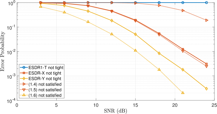
Figure 2: Error probabilities versus the SNR in a $16\times 10$ MIMO system with 8-PSK.

We can see from Fig. 2 that our results Eqs. 5 and 6 provide better characterizations than the previous tightness condition Eq. 4 in [16]. The empirical probability of Eq. ESDR-${\mathbf{X}}$ not being tight matches perfectly with our analysis given by the necessary and sufficient condition Eq. 5. The probability of Eq. 6 not being satisfied is also a good approximation to the probability of Eq. ESDR-${\mathbf{Y}}$ not being tight, underestimating the latter roughly by a factor of 9. Moreover, the numerical results also validate our analysis that Eq. ESDR1-${\mathbf{T}}$ is not tight with high probability. In fact, Eq. ESDR1-${\mathbf{T}}$ fails to recover the vector of transmitted symbols in all 80,000 instances.

Next, we compare the optimal values as well as the CPU time of solving Eq. ESDR-${\mathbf{Y}}$ and Eq. ESDR2-${\mathbf{T}}$. Table 2 shows the relative difference between the optimal values of Eq. ESDR-${\mathbf{Y}}$ (denoted as $\mathrm{opt}_{\text{ESDR-}{\mathbf{Y}}}$) and Eq. ESDR2-${\mathbf{T}}$ (denoted as $\mathrm{opt}_{\text{ESDR2-}{\mathbf{T}}}$) averaged over 300 simulations, which is defined as $|\mathrm{opt}_{\text{ESDR-}{\mathbf{Y}}}-\mathrm{opt}_{\text{ESDR2-}{\mathbf{T}}}|/|\mathrm{opt}_{\text{ESDR2-}{\mathbf{T}}}|$. We can see from Table 2 that the difference is consistently in the order 1e$-$7 in various settings, which verifies the equivalence between Eq. ESDR-${\mathbf{Y}}$ and Eq. ESDR2-${\mathbf{T}}$. In Fig. 3, we plot the average CPU time consumed by solving Eq. ESDR-${\mathbf{Y}}$ and Eq. ESDR2-${\mathbf{T}}$ in an 8-PSK system with increasing problem size $n$. For fair comparison, both SDRs are implemented and solved by SeDuMi and we repeat the simulations for 300 times. With the same error performance, we can see that Eq. ESDR-${\mathbf{Y}}$ indeed solves the MIMO detection problem Eq. 2 more efficiently and saves roughly 90% of the computational time in our experiment.

Table 2: Average relative difference between Eq. ESDR-${\mathbf{Y}}$ and Eq. ESDR2-${\mathbf{T}}$ in optimal objective values.

SNR	Relative diff. in optimal objective values.
	$(m,n)=(4,4)$	$(m,n)=(6,4)$	$(m,n)=(10,10)$	$(m,n)=(15,10)$
5dB	4.62e$-$7	5.10e$-$7	6.26e$-$7	7.73e$-$7
10dB	5.67e$-$7	4.06e$-$7	6.50e$-$7	7.16e$-$7
15dB	5.94e$-$7	3.83e$-$7	7.80e$-$7	5.58e$-$7

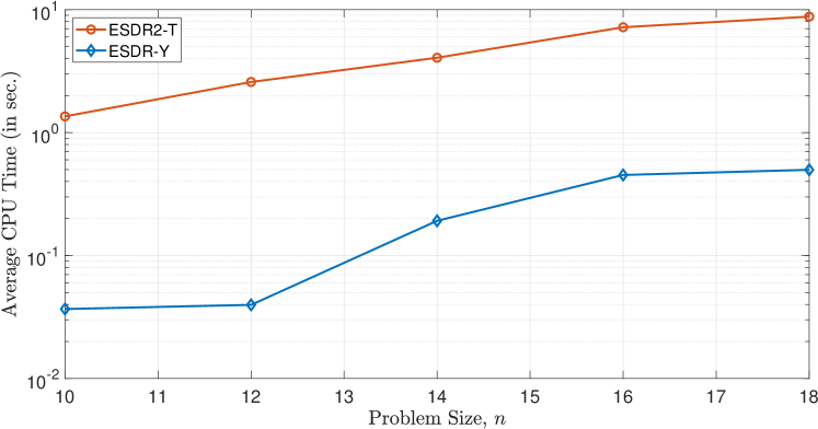
Figure 3: Average CPU time of solving Eq. ESDR-${\mathbf{Y}}$ and Eq. ESDR2-${\mathbf{T}}$ when $M=8$.

6 Conclusions

In this paper, we studied the tightness and equivalence of various existing SDR models for the MIMO detection problem Eq. 2. For the two SDRs Eq. ESDR-${\mathbf{X}}$ and Eq. ESDR-${\mathbf{Y}}$ proposed in [17], we improved their sufficient tightness condition and showed that the former is tight if and only if Eq. 5 holds while the latter is tight only if Eq. 6 holds. On the other hand, for the SDR Eq. ESDR1-${\mathbf{T}}$ proposed in [22], we proved that its tightness probability decays to zero exponentially fast with an increasing problem size under some mild assumptions. Together with known results, our analysis provides a more complete understanding of the tightness conditions for existing SDRs. Moreover, we proposed a general theorem that unifies previous results on the equivalence of SDRs [21, 16]. For a subset of PSD matrices with a special “separable” structure, we showed its equivalence to another subset of PSD matrices in a potentially much smaller dimension. Our numerical results demonstrated that we could significantly improve the computational efficiency by using such equivalence.

Due to its generality, we believe that our equivalence theorem can be applied to SDPs in other domains beyond MIMO detection and we would like to put this as a future work. Additionally, we noticed that the SDRs for problem Eq. 2 combined with some simple rounding procedure can detect the transmitted symbols successfully even when the optimal solution has rank more than one. Similar observations have also been made in [12]. It would be interesting to extend our analysis to take the postprocessing procedure into account.

Appendix A Simplification of Eqs. 21 and 22

Fix $i\in\{1,2,\ldots,n\}$. From Eq. 21, we have

$$(\hat{{\mathbf{H}}}^{\mathsf{T}}\hat{{\bm{v}}})_{i}=g_{i}+\lambda_{i}y_{i}^{*}+\mu_{i}y_{n+i}^{*}\;\text{and}\;(\hat{{\mathbf{H}}}^{\mathsf{T}}\hat{{\bm{v}}})_{n+i}=g_{n+i}+\mu_{i}y_{i}^{*}+\lambda_{n+i}y_{n+i}^{*},$$

which can be written in a matrix form:

(56) $$\begin{bmatrix}(\hat{{\mathbf{H}}}^{\mathsf{T}}\hat{{\bm{v}}})_{i}\\ (\hat{{\mathbf{H}}}^{\mathsf{T}}\hat{{\bm{v}}})_{n+i}\end{bmatrix}=\begin{bmatrix}g_{i}\\ g_{n+i}\end{bmatrix}+\begin{bmatrix}\lambda_{i}&\mu_{i}\\ \mu_{i}&\lambda_{n+i}\end{bmatrix}\begin{bmatrix}y_{i}^{*}\\ y_{n+i}^{*}\end{bmatrix}.$$

Recall the definitions of ${\mathbf{\Gamma}}_{i}$ in Eq. 23 and ${\mathbf{K}}_{j}$ in Eq. 12. Then

(57) $$\langle{\mathbf{\Gamma}}_{i},{\mathbf{K}}_{j}\rangle=2\begin{bmatrix}\cos(\theta_{j})\\ \sin(\theta_{j})\end{bmatrix}^{\mathsf{T}}\begin{bmatrix}g_{i}\\ g_{n+i}\end{bmatrix}+\begin{bmatrix}\cos(\theta_{j})\\ \sin(\theta_{j})\end{bmatrix}^{\mathsf{T}}\begin{bmatrix}\lambda_{i}&\mu_{i}\\ \mu_{i}&\lambda_{n+i}\end{bmatrix}\begin{bmatrix}\cos(\theta_{j})\\ \sin(\theta_{j})\end{bmatrix}.$$

Using Eq. 56, we have

(58) $$\begin{bmatrix}\cos(\theta_{j})\\ \sin(\theta_{j})\end{bmatrix}^{\mathsf{T}}\begin{bmatrix}g_{i}\\ g_{n+i}\end{bmatrix} =\begin{bmatrix}\cos(\theta_{j})\\ \sin(\theta_{j})\end{bmatrix}^{\mathsf{T}}\begin{bmatrix}(\hat{{\mathbf{H}}}^{\mathsf{T}}\hat{{\bm{v}}})_{i}\\ (\hat{{\mathbf{H}}}^{\mathsf{T}}\hat{{\bm{v}}})_{n+i}\end{bmatrix}-\begin{bmatrix}\cos(\theta_{j})\\ \sin(\theta_{j})\end{bmatrix}^{\mathsf{T}}\begin{bmatrix}\lambda_{i}&\mu_{i}\\ \mu_{i}&\lambda_{n+i}\end{bmatrix}\begin{bmatrix}y_{i}^{*}\\ y_{n+i}^{*}\end{bmatrix}$$

$$=\begin{bmatrix}\cos(\Delta\theta_{j})\\ \sin(\Delta\theta_{j})\end{bmatrix}^{\mathsf{T}}\begin{bmatrix}\hat{z}_{i}\\ \hat{z}_{n+i}\end{bmatrix}-\begin{bmatrix}\cos(\theta_{j})\\ \sin(\theta_{j})\end{bmatrix}^{\mathsf{T}}\begin{bmatrix}\lambda_{i}&\mu_{i}\\ \mu_{i}&\lambda_{n+i}\end{bmatrix}\begin{bmatrix}y_{i}^{*}\\ y_{n+i}^{*}\end{bmatrix},$$

where $\Delta\theta_{j}=\theta_{j}-\theta_{u_{i}}$, $\hat{z}_{i}={\mathrm{Re}}(z_{i})$, and $\hat{z}_{n+i}={\mathrm{Im}}(z_{i})$ (cf. Eq. 17). Combining Eq. 57 with Eq. 58, we get

$$\langle{\mathbf{\Gamma}}_{i},{\mathbf{K}}_{j}\rangle =2\begin{bmatrix}\cos(\Delta\theta_{j})\\ \sin(\Delta\theta_{j})\end{bmatrix}^{\mathsf{T}}\begin{bmatrix}\hat{z}_{i}\\ \hat{z}_{n+i}\end{bmatrix}-2\begin{bmatrix}\cos(\theta_{j})\\ \sin(\theta_{j})\end{bmatrix}^{\mathsf{T}}\begin{bmatrix}\lambda_{i}&\mu_{i}\\ \mu_{i}&\lambda_{n+i}\end{bmatrix}\begin{bmatrix}y_{i}^{*}\\ y_{n+i}^{*}\end{bmatrix}+$$

$$\phantom{=}\;\begin{bmatrix}\cos(\theta_{j})\\ \sin(\theta_{j})\end{bmatrix}^{\mathsf{T}}\begin{bmatrix}\lambda_{i}&\mu_{i}\\ \mu_{i}&\lambda_{n+i}\end{bmatrix}\begin{bmatrix}\cos(\theta_{j})\\ \sin(\theta_{j})\end{bmatrix}.$$

In particular, when $j=u_{i}$, the above becomes

$$\langle{\mathbf{\Gamma}}_{i},{\mathbf{K}}_{u_{i}}\rangle=2\begin{bmatrix}1\\ 0\end{bmatrix}^{\mathsf{T}}\begin{bmatrix}\hat{z}_{i}\\ \hat{z}_{n+i}\end{bmatrix}-\begin{bmatrix}y_{i}^{*}\\ y_{n+i}^{*}\end{bmatrix}^{\mathsf{T}}\begin{bmatrix}\lambda_{i}&\mu_{i}\\ \mu_{i}&\lambda_{n+i}\end{bmatrix}\begin{bmatrix}y_{i}^{*}\\ y_{n+i}^{*}\end{bmatrix}.$$

Hence, when $j\neq u_{i}$, Eq. 22 is equivalent to

$$2\begin{bmatrix}1-\cos(\Delta\theta_{j})\\ -\sin(\Delta\theta_{j})\end{bmatrix}^{\mathsf{T}}\begin{bmatrix}\hat{z}_{i}\\ \hat{z}_{n+i}\end{bmatrix} \geq\begin{bmatrix}y_{i}^{*}-\cos(\theta_{j})\\ y_{n+i}^{*}-\sin(\theta_{j})\end{bmatrix}^{\mathsf{T}}\begin{bmatrix}\lambda_{i}&\mu_{i}\\ \mu_{i}&\lambda_{n+i}\end{bmatrix}\begin{bmatrix}y_{i}^{*}-\cos(\theta_{j})\\ y_{n+i}^{*}-\sin(\theta_{j})\end{bmatrix}$$

$$\Leftrightarrow\begin{bmatrix}1\\ -\cot\left(\frac{\Delta\theta_{j}}{2}\right)\end{bmatrix}^{\mathsf{T}}\begin{bmatrix}\hat{z}_{i}\\ \hat{z}_{n+i}\end{bmatrix} \geq\begin{bmatrix}\sin(\theta_{u_{i}}+\frac{\Delta\theta_{j}}{2})\\ -\cos(\theta_{u_{i}}+\frac{\Delta\theta_{j}}{2})\end{bmatrix}^{\mathsf{T}}\begin{bmatrix}\lambda_{i}&\mu_{i}\\ \mu_{i}&\lambda_{n+i}\end{bmatrix}\begin{bmatrix}\sin(\theta_{u_{i}}+\frac{\Delta\theta_{j}}{2})\\ -\cos(\theta_{u_{i}}+\frac{\Delta\theta_{j}}{2})\end{bmatrix},$$

which is exactly the same as Eq. 24.

Appendix B Proof of Lemma 4.5

To simplify the notations, we use $\mathcal{A}$ and $\mathcal{B}$ to denote the left-hand side and the right-hand side in Eq. 55, respectively.

We first prove that $\mathcal{A}\supset\mathcal{B}$. Let $\mathcal{C}=\bigl{\{}{\mathbf{B}}\in\mathbb{S}_{+}^{q}:\;\operatorname{diag}({\mathbf{B}})={\bm{1}}_{q}\bigr{\}}$, and we can view $\mathcal{A}$ as the image of the convex set $\mathcal{C}$ under the affine mapping ${\mathbf{B}}\mapsto\langle{\mathbf{B}},{\bm{w}}{\bm{w}}^{\mathsf{T}}\rangle$. Therefore, the set $\mathcal{A}$ is also convex. Moreover, note that both the rank-one matrices ${\bm{1}}_{q}{\bm{1}}_{q}^{\mathsf{T}}$ and $[\begin{smallmatrix}-{\bm{1}}_{q-1}\\ 1\end{smallmatrix}][\begin{smallmatrix}-{\bm{1}}_{q-1}\\ 1\end{smallmatrix}]^{\mathsf{T}}$ belong to $\mathcal{C}$. Direct computations show that

$${\bm{w}}^{\mathsf{T}}{\bm{1}}_{q}{\bm{1}}_{q}^{\mathsf{T}}{\bm{w}} =\biggl{(}\sum_{i=1}^{q}2^{i-1}\biggr{)}^{2}=(2^{q}-1)^{2},$$

$${\bm{w}}^{\mathsf{T}}\begin{bmatrix}-{\bm{1}}_{q-1}\\ 1\end{bmatrix}\begin{bmatrix}-{\bm{1}}_{q-1}\\ 1\end{bmatrix}^{\mathsf{T}}{\bm{w}} =\biggl{(}2^{q-1}-\sum_{i=1}^{q-1}2^{i-1}\biggr{)}^{2}=1,$$

and hence both $1$ and $(2^{q}-1)^{2}$ belong to $\mathcal{A}$. Finally, the convexity of $\mathcal{A}$ implies $\mathcal{B}\subset\mathcal{A}$.

Now we prove the other direction, i.e., $\mathcal{A}\subset\mathcal{B}$. This is equivalent to showing

$$1\leq{\bm{w}}^{\mathsf{T}}{\mathbf{B}}{\bm{w}}\leq(2^{q}-1)^{2},\;\forall\;{\mathbf{B}}\in\mathcal{C}.$$

For the upper bound, we first note that ${\mathbf{B}}\in\mathbb{S}_{+}^{q}$ implies

(59) $$|B_{i,j}|\leq\sqrt{B_{i,i}B_{j,j}}=1,\;\;\;i\neq j,\;1\leq i,j\leq q.$$

Since every entry of the matrix ${\bm{w}}{\bm{w}}^{\mathsf{T}}$ is positive, we have

$${\bm{w}}^{\mathsf{T}}{\mathbf{B}}{\bm{w}}=\langle{\mathbf{B}},{\bm{w}}{\bm{w}}^{\mathsf{T}}\rangle\leq\langle{\bm{1}}{\bm{1}}^{\mathsf{T}},{\bm{w}}{\bm{w}}^{\mathsf{T}}\rangle=(2^{q}-1)^{2}$$

for any ${\mathbf{B}}\in\mathcal{C}$, and hence the upper bound holds.

For the lower bound, it clearly holds when $q=1$. When $q>1$, for any matrix ${{\mathbf{B}}}\in\mathcal{C}$ we partition it as

$${{\mathbf{B}}}=\begin{bmatrix}{\mathbf{B}}^{\prime}&{\bm{b}}^{\prime}\\ ({\bm{b}}^{\prime})^{\mathsf{T}}&1\end{bmatrix},$$

where ${\mathbf{B}}^{\prime}\in\mathbb{R}^{(q-1)\times(q-1)}$ and ${\bm{b}}^{\prime}\in\mathbb{R}^{q-1}$. Note that we have $|b^{\prime}_{i}|\leq 1$ for $1\leq i\leq q-1$ (cf. Eq. 59), and ${\mathbf{B}}\in\mathbb{S}_{+}^{q}$ implies ${\mathbf{B}}^{\prime}\succeq{\bm{b}}^{\prime}({\bm{b}}^{\prime})^{\mathsf{T}}$. Further, we let ${{\bm{w}}}^{\prime}=\begin{bmatrix}1&2&4&\ldots&2^{q-2}\end{bmatrix}^{\mathsf{T}}\in\mathbb{R}^{q-1}$ such that ${\bm{w}}=[({\bm{w}}^{\prime})^{\mathsf{T}}\quad 2^{q-1}]^{\mathsf{T}}$ (cf. Eq. 49). We have

$${{\bm{w}}}^{\mathsf{T}}{{\mathbf{B}}}{{\bm{w}}} =({\bm{w}}^{\prime})^{\mathsf{T}}{\mathbf{B}}{\bm{w}}^{\prime}+2^{q}({\bm{w}}^{\prime})^{\mathsf{T}}{\bm{b}}^{\prime}+(2^{q-1})^{2}$$

$$\geq({\bm{w}}^{\prime})^{\mathsf{T}}{\bm{b}}^{\prime}({\bm{b}}^{\prime})^{\mathsf{T}}{\bm{w}}^{\prime}+2^{q}({\bm{w}}^{\prime})^{\mathsf{T}}{\bm{b}}^{\prime}+(2^{q-1})^{2}$$

$$=\bigl{(}({\bm{w}}^{\prime})^{\mathsf{T}}{\bm{b}}^{\prime}+2^{q-1}\bigr{)}^{2}.$$

Since

$$({\bm{w}}^{\prime})^{\mathsf{T}}{\bm{b}}^{\prime}=\sum_{i=1}^{q-1}2^{i-1}b^{\prime}_{i}\geq-\sum_{i=1}^{q-1}2^{i-1}=-2^{q-1}+1,$$

we immediately get ${{\bm{w}}}^{\mathsf{T}}{{\mathbf{B}}}{{\bm{w}}}\geq(-2^{q-1}+1+2^{q-1})^{2}=1$, and hence the lower bound also holds.

The proof is now complete.

References

- [1] A. S. Bandeira, N. Boumal, and A. Singer, Tightness of the maximum likelihood semidefinite relaxation for angular synchronization, Math. Program., 163 (2017), pp. 145–167.
- [2] P. Biswas, T.-C. Lian, T.-C. Wang, and Y. Ye, Semidefinite programming based algorithms for sensor network localization, ACM Trans. Sen. Netw., 2 (2006), pp. 188–220.
- [3] P. Biswas and Y. Ye, Semidefinite programming for ad hoc wireless sensor network localization, in Proceedings of the 3rd International Symposium on Information Processing in Sensor Networks (IPSN’04), New York, NY, 2004, ACM, pp. 46–54.
- [4] O. Damen, A. Chkeif, and J.-C. Belfiore, Lattice code decoder for space-time codes, IEEE Commun. Lett., 4 (2000), pp. 161–163.
- [5] A. Duel-Hallen, Decorrelating decision-feedback multiuser detector for synchronous code-division multiple-access channel, IEEE Trans. Commun., 41 (1993), pp. 285–290.
- [6] G. J. Foschini, Layered space-time architecture for wireless communication in a fading environment when using multi-element antennas, Bell Labs Tech. J., 1 (1996), pp. 41–59.
- [7] M. X. Goemans and D. P. Williamson, Improved approximation algorithms for maximum cut and satisfiability problems using semidefinite programming, J. ACM, 42 (1995), pp. 1115–1145.
- [8] R. A. Horn and C. R. Johnson, Matrix Analysis, Cambridge University Press, New York, USA, 2nd ed., 2013.
- [9] J. Jaldén, Detection for Multiple Input Multiple Output Channels, PhD thesis, School of Electrical Engineering, KTH, Stockholm, Sweden, 2006.
- [10] J. Jaldén, C. Martin, and B. Ottersten, Semidefinite programming for detection in linear systems - Optimality conditions and space-time decoding, in Proceedings of the IEEE International Conference on Acoustics, Speech, and Signal Processing (ICASSP’03), Piscataway, NJ, 2003, IEEE Press, pp. 9–12.
- [11] J. Jaldén and B. Ottersten, On the complexity of sphere decoding in digital communications, IEEE Trans. Signal Process., 53 (2005), pp. 1474–1484.
- [12] J. Jaldén and B. Ottersten, The diversity order of the semidefinite relaxation detector, IEEE Trans. Inf. Theory, 54 (2008), pp. 1406–1422.
- [13] R. Jiang, Y.-F. Liu, C. Bao, and B. Jiang, A companion technical report of “tightness and equivalence of semidefinite relaxations for MIMO detection”, tech. report, Academy of Mathematics and Systems Science, Chinese Academy of Sciences, 2020, http://lsec.cc.ac.cn/~yafliu/Technical_Report_MIMO.pdf.
- [14] M. Kisialiou and Z.-Q. Luo, Performance analysis of quasi-maximum-likelihood detector based on semi-definite programming, in Proceedings of the IEEE International Conference on Acoustics, Speech and Signal Processing (ICASSP’05), Piscataway, NJ, 2005, IEEE Press, pp. 433–436.
- [15] Y.-F. Liu, M. Hong, and Y.-H. Dai, Max-Min fairness linear transceiver design problem for a multi-user SIMO interference channel is polynomial time solvable, IEEE Signal Process. Lett., 20 (2013), pp. 27–30.
- [16] Y.-F. Liu, Z. Xu, and C. Lu, On the equivalence of semidifinite relaxations for MIMO detection with general constellations, in Proceedings of the IEEE International Conference on Acoustics, Speech and Signal Processing (ICASSP’19), Piscataway, NJ, 2019, IEEE Press, pp. 4549–4553.
- [17] C. Lu, Y.-F. Liu, W.-Q. Zhang, and S. Zhang, Tightness of a new and enhanced semidefinite relaxation for MIMO detection, SIAM J. Optim., 29 (2019), pp. 719–742.
- [18] Z.-Q. Luo, W.-K. Ma, A. M.-C. So, Y. Ye, and S. Zhang, Semidefinite relaxation of quadratic optimization problems, IEEE Signal Process. Mag., 27 (2010), pp. 20–34.
- [19] W.-K. Ma, P.-C. Ching, and Z. Ding, Semidefinite relaxation based multiuser detection for M-ary PSK multiuser systems, IEEE Trans. Signal Process., 52 (2004), pp. 2862–2872.
- [20] W.-K. Ma, T. N. Davidson, K. M. Wong, Z.-Q. Luo, and P.-C. Ching, Quasi-maximum-likelihood multiuser detection using semi-definite relaxation with application to synchronous CDMA, IEEE Trans. Signal Process., 50 (2002), pp. 912–922.
- [21] W.-K. Ma, C.-C. Su, J. Jaldén, T.-H. Chang, and C.-Y. Chi, The equivalence of semidefinite relaxation MIMO detectors for higher-order QAM, IEEE J. Sel. Top. Signal Process., 3 (2009), pp. 1038–1052.
- [22] A. Mobasher, M. Taherzadeh, R. Sotirov, and A. K. Khandani, A near-maximum-likelihood decoding algorithm for MIMO systems based on semi-definite programming, IEEE Trans. Inf. Theory, 53 (2007), pp. 3869–3886.
- [23] K. S. Schneider, Optimum detection of code division multiplexed signals, IEEE Trans. Aerosp. Electron. Syst., 15 (1979), pp. 181–185.
- [24] N. D. Sidiropoulos, T. N. Davidson, and Z.-Q. Luo, Transmit beamforming for physical-layer multicasting, IEEE Trans. Signal Process., 54 (2006), pp. 2239–2251.
- [25] A. Singer, Angular synchronization by eigenvectors and semidefinite programming, Appl. Comput. Harmon. Anal., 30 (2011), pp. 20–36.
- [26] A. M.-C. So, Probabilistic analysis of the semidefinite relaxation detector in digital communications, in Proceedings of the Twenty-First Annual ACM-SIAM Symposium on Discrete Algorithms (SODA’10), Philadelphia, PA, 2011, SIAM, pp. 698–711.
- [27] A. M.-C. So and Y. Ye, Theory of semidefinite programming for sensor network localization, Math. Program., 109 (2007), pp. 367–384.
- [28] B. Steingrimsson, Z.-Q. Luo, and K. M. Wong, Soft quasi-maximum-likelihood detection for multiple-antenna wireless channels, IEEE Trans. Signal Process., 51 (2003), pp. 2710–2719.
- [29] J. F. Sturm, Using SeDuMi 1.02, a MATLAB toolbox for optimization over symmetric cones, Optim. Methods Softw., 11 (1999), pp. 625–653.
- [30] P. H. Tan and L. K. Rasmussen, The application of semidefinite programming for detection in CDMA, IEEE J. Sel. Areas Commun., 19 (2001), pp. 1442–1449.
- [31] D. Tse and P. Viswanath, Fundamentals of Wireless Communication, Cambridge University Press, New York, 2005.
- [32] S. Verdú, Computational complexity of optimum multiuser detection, Algorithmica, 4 (1989), pp. 303–312.
- [33] S. Verdú, Multiuser Detection, Cambridge University Press, New York, 1998.
- [34] I. Waldspurger, A. D’Aspremont, and S. Mallat, Phase recovery, MaxCut and complex semidefinite programming, Math. Program., 149 (2015), pp. 47–81.
- [35] Z. Xie, R. T. Short, and C. K. Rushforth, A family of suboptimum detectors for coherent multiuser communications, IEEE J. Sel. Areas Commun., 8 (1990), pp. 683–690.
- [36] S. Yang and L. Hanzo, Fifty years of MIMO detection: The road to large-scale MIMOs, IEEE Commun. Surveys Tuts., 17 (2015), pp. 1941–1988.
- [37] Y. Zhong and N. Boumal, Near-optimal bounds for phase synchronization, SIAM J. Optim., 28 (2018), pp. 989–1016.