Finding Nash Equilibria of Two-Player Games

Abstract

This paper is an exposition of algorithms for finding one or all equilibria of a bimatrix game (a two-player game in strategic form) in the style of a chapter in a graduate textbook. Using labeled “best-response polytopes”, we present the Lemke-Howson algorithm that finds one equilibrium. We show that the path followed by this algorithm has a direction, and that the endpoints of the path have opposite index, in a canonical way using determinants. For reference, we prove that a number of notions of nondegeneracy of a bimatrix game are equivalent. The computation of all equilibria of a general bimatrix game, via a description of the maximal Nash subsets of the game, is canonically described using “complementary pairs” of faces of the best-response polytopes.

1   Introduction

A bimatrix game is a two-player game in strategic form, specified by the two matrices of payoffs to the row player and column player. This article describes algorithms that find one or all Nash equilibria of such a game.

The game gives rise to two suitably labeled polytopes (described in Section 3), which help finding its Nash equilibria. This geometric structure is also very informative and accessible, for example for the construction of $3\times 3$ games with a certain equilibrium structure, which is much more varied than for $2\times 2$ games. It also provides an elementary and constructive proof for the existence of a Nash equilibrium for a bimatrix game via the algorithm by Lemke and Howson (1964). In Section 4, we first explain this algorithm following the exposition by Shapley (1974), in particular using the subdivision of the mixed strategy simplices $X$ and $Y$ into best-response regions, and the construction of $\tilde{X}$ and $\tilde{Y}$ in Section 4 and Figure 5, which extends $X\times Y$ with an “artificial equilibrium”. In Section 5, we then give a more concise description using polytopes. Section 6 gives a canonical proof that the endpoints of Lemke-Howson paths have opposite index. The index is here defined in an elementary way using determinants (Definition 11). In Section 7, we show that a number of known definitions of nondegeneracy of a bimatrix game are in fact equivalent. Section 8 shows how to implement the Lemke-Howson algorithm by “complementary pivoting”, even when the game is degenerate. Section 9 describes the structure of Nash equilibria of a general bimatrix game.

An undergraduate text, in even more detailed style and avoiding advanced mathematical machinery, is von Stengel (2021). This article continues Chapter 9 of that book, with the proof of the direction of a Lemke–Howson path and the concept of the index of an equilibrium, and the detailed discussion of nondegeneracy. Earlier expositions of this topic are von Stengel (2002), which gives additional historical references, and von Stengel (2007). Compared to these surveys, the following expository results are new:

$\bullet$ The definition of the index of a Nash equilibrium in a nondegenerate game, and the very canonical proof that opposite endpoints of Lemke-Howson paths have opposite index in Theorem 13. Essentially, this is a much more accessible version of the argument by Shapley (1974).

$\bullet$ The equivalent definitions of nondegeneracy in Theorem 14.

$\bullet$ A cleaner presentation of maximal Nash subsets, adapted from Avis, Rosenberg, Savani, and von Stengel (2010), in Proposition 17.

2   Bimatrix games and the best response condition

We use the following notation throughout. Let $(A,B)$ be an $m\times n$ bimatrix game, that is, $A$ and $B$ are $m\times n$ matrices of payoffs to the row player 1 and column player 2, respectively. This is a two-player game in strategic form (also called “normal form”), which is played by a simultaneous choice of a row $i$ by player 1 and column $j$ by player 2, who then receive the entries $a_{ij}$ of the matrix $A$, and $b_{ij}$ of $B$, as respective payoffs. The payoffs represent risk-neutral utilities, so when facing a probability distribution, the players want to maximize their expected payoff. These preferences do not depend on positive-affine transformations, so that $A$ and $B$ can be assumed to have nonnegative entries. In addition, as inputs to an algorithm they are assumed to be rationals or just integers.

All vectors are column vectors, so an $m$-vector vector $x$ (that is, an element of $\mathbb{R}^{m}$) is treated as an $m\times 1$ matrix, with components $x_{1},\ldots,x_{m}$. A scalar is treated as a $1\times 1$ matrix, and therefore multiplied to the right of a column vector and to the left of a row vector. A mixed strategy $x$ for player 1 is a probability distribution on the rows of the game, written as an $m$-vector of probabilities. Similarly, a mixed strategy $y$ for player 2 is an $n$-vector of probabilities for playing the columns of the game. Let 0 be the all-zero vector and let 1 be the all-one vector of appropriate dimension. The transpose of any matrix $C$ is denoted by $C^{\kern-0.27995pt\top\kern-0.70004pt}$, so $\textup{{1}}^{\kern-0.27995pt\top\kern-0.70004pt}$ is the all-one row vector. Inequalities like $x\geq\bf 0$ between two vectors hold for all components. Let $X$ and $Y$ be the mixed-strategy sets of the two players,

$$X=\{x\in\mathbb{R}^{m}\mid x\geq\textup{{0}},~{}\textup{{1}}^{\kern-0.27995pt\top\kern-0.70004pt}x=1\,\},\qquad Y=\{y\in\mathbb{R}^{n}\mid y\geq\textup{{0}},~{}\textup{{1}}^{\kern-0.27995pt\top\kern-0.70004pt}y=1\,\}.$$ (1)

The support $\textup{\small{supp}}(z)$ of a mixed strategy $z$ is the set of pure strategies that have positive probability, so $\textup{\small{supp}}(z)=\{\,k\mid z_{k}>0\}$.

A best response to the mixed strategy $y$ of player 2 is a mixed strategy $x$ of player 1 that maximizes his expected payoff $x^{\top}Ay$. Similarly, a best response $y$ of player 2 to $x$ maximizes her expected payoff $x^{\top}By$. A Nash equilibrium or just equilibrium is a pair $(x,y)$ of mixed strategies that are best responses to each other. The following proposition states that a mixed strategy $x$ is a best response to an opponent strategy $y$ if and only if all pure strategies in its support are pure best responses to $y$. The same holds with the roles of the players exchanged.

Proposition 1 (Best response condition).

Let $x$ and $y$ be mixed strategies of player $1$ and $2$, respectively. Then $x$ is a best response to $y$ if and only if for all $i=1,\ldots,m$,

$$x_{i}>0~{}~{}\Rightarrow~{}~{}(Ay)_{i}=u=\max\{\,(Ay)_{k}\mid k=1,\ldots,m\}.$$ (2)

Proof. $(Ay)_{i}$ is the $i$th component of $Ay$, which is the expected payoff to player 1 when playing row $i$. Then

$$x^{\top}Ay=\sum_{i=1}^{m}x_{i}\,(Ay)_{i}=\sum_{i=1}^{m}x_{i}\,(u-(u-(Ay)_{i})=u-\sum_{i=1}^{m}x_{i}\,(u-(Ay)_{i}).$$

So $x^{\top}Ay\leq u$ because $x_{i}\geq 0$ and $u-(Ay)_{i}\geq 0$ for all $i=1,\ldots,m$, and $x^{\top}Ay=u$ if and only if $x_{i}>0$ implies $(Ay)_{i}=u$, as claimed.     

Proposition 1 is useful in a number of respects. First, by definition, $x$ is a best response to $y$ if and only if $x^{\kern-0.27995pt\top\kern-0.70004pt}Ay\geq\hat{x}^{\kern-0.27995pt\top\kern-0.70004pt}Ay$ for all other mixed strategies $\hat{x}$ in $X$ of player 1, where $X$ is an infinite set. In contrast, (2) is a finite condition, which only concerns the pure strategies $i$ of player 1, which have to give maximum payoff $(Ay)_{i}$ whenever $x_{i}>0$. For example, in the $3\times 2$ game

$$A=\left[\,\begin{matrix}3&3\cr 2&5\cr 0&6\cr\end{matrix}\,\right],\qquad B=\left[\,\begin{matrix}3&2\cr 2&4\cr 3&0\cr\end{matrix}\,\right],$$ (3)

if $y=(\frac{1}{3},\frac{2}{3})^{\kern-0.27995pt\top\kern-0.70004pt}$, then $Ay=(3,4,4)^{\kern-0.27995pt\top\kern-0.70004pt}$. (From now on, we omit for brevity the transposition when writing down specific vectors, as in $y=(\frac{1}{3},\frac{2}{3})$.) Then player 1’s pure best responses against $y$ are the second and third row, and $x=(x_{1},x_{2},x_{3})$ in $X$ is a best response to $y$ if and only if $x_{1}=0$. In order for $x$ to be a best response against $y$, the pure best responses $2$ and $3$ can be played with arbitrary probabilities $x_{2}$ and $x_{3}$. (As part of an equilibrium these probabilities will here be unique in order to ensure the best response condition for the other player.) Second, as the proof of Proposition 1 shows, mixing cannot improve the payoff of a player (here of player 1), which is just a “weighted average” of the expected payoffs $(Ay)_{i}$ with the weights $x_{i}$ for the rows $i$. This payoff is maximal only if only the maximum pure-strategy payoffs $(Ay)_{i}$ have positive weight.

We denote by $\textup{\small{bestresp}}(z)$ the set of pure best responses of a player against a mixed strategy $z$ of the other player, so $\textup{\small{bestresp}}(y)\subseteq\{1,\ldots,m\}$ if $y\in Y$ and $\textup{\small{bestresp}}(x)\subseteq\{1,\ldots,n\}$ if $x\in X$. Then (2) states that $x$ is a best response to $y$ if and only if

$$\textup{\small{supp}}(x)\subseteq\textup{\small{bestresp}}(y).$$ (4)

This condition applies also to games with any finite number of players: If $s$ is any one of $N$ players who plays the mixed strategy $x^{s}$, with the tuple of the ${N-1}$ mixed strategies of the remaining players denoted by $x^{-s}$, then $x^{s}$ is a best response against $x^{-s}$ if and only if

$$\textup{\small{supp}}(x^{s})\subseteq\textup{\small{bestresp}}(x^{-s}).$$ (5)

The proof of Proposition 1 still applies, where instead of $(Ay)_{i}$ for a pure strategy $i$ of player $s$ one has to use the expected payoff to player $s$ when he uses strategy $i$ against the tuple $x^{-s}$ of mixed strategies of the other players. For more than two players, $N>2$, that expected payoff involves products of the mixed strategy probabilities $x^{r}$ for the other players $r$ in $N-\{s\}$ and is therefore nonlinear. The resulting polynomial equations and inequalities make the structure and computation of Nash equilibria for such games much more complicated than for two players, where the expected payoffs $(Ay)_{i}$ are linear in the opponent’s mixed strategy $y$. We consider only two-player games here.

Proposition 1 is used in algorithms that find Nash equilibria of the game. One such approach is to consider the different possible supports of mixed strategies. All pure strategies in the support must have maximum, and hence equal, expected payoff to that player. This leads to equations for the probabilities of the opponent’s mixed strategy. In the above example (3), the mixed strategy $y=(\frac{1}{3},\frac{2}{3})$ has any $x=(0,x_{2},x_{3})\geq\textup{{0}}$ with $x_{2}+x_{3}=1$ as a best response. In order for $y$ to be a best response against such an $x$, the two columns have to have maximal and hence equal payoff to player 2, that is, $2x_{2}+3x_{3}=4x_{2}+0x_{3}$, which has the unique solution $x_{2}=\frac{3}{5}$, $x_{3}=\frac{2}{5}$ and expected payoff $\frac{12}{5}$ to player 2. Hence, $(x,y)$ is an equilibrium, which we denote for later reference by $(a,c)$,

$$\textstyle(a,c)=((0,\frac{3}{5},\frac{2}{5}),(\frac{1}{3},\frac{2}{3})).$$ (6)

Here the mixed strategy $y$ of player 2 is uniquely determined by the condition $2y_{1}+5y_{2}=0y_{1}+6y_{2}$ that the two bottom rows give equal expected payoff to player 1.

A second mixed equilibrium $(x,y)$ is given if the support of player 1’s strategy consists of the first two rows, which gives the equation $3y_{1}+3y_{2}=2y_{1}+5y_{2}$ with the unique solution $y=(\frac{2}{3},\frac{1}{3})$ and thus $Ay=(3,3,2)$. With $x=(x_{1},x_{2},0)$ the equal payoffs to player 2 for her two columns give the equation $3x_{1}+2x_{2}=2x_{1}+4x_{2}$ with unique solution $x=(\frac{2}{3},\frac{1}{3},0)$. Then $(x,y)$ is an equilibrium, for later reference denoted by $(b,d)$,

$$\textstyle(b,d)=((\frac{2}{3},\frac{1}{3},0),(\frac{2}{3},\frac{1}{3})).$$ (7)

A third, pure-strategy Nash equilibrium of the game is $((1,0,0),(1,0))$.

The support set $\{1,3\}$ for the mixed strategy of player 1 does not lead to an equilibrium, for two reasons. First, player 2 would have to play $y=(\frac{1}{2},\frac{1}{2})$ to make player 1 indifferent between row 1 and row 3. But then the vector of expected payoffs to player 1 is $Ay=(3,\frac{7}{2},3)$, so that rows 1 and 3 give the same payoff to player 1 but not the maximum payoff for all rows. Second, player 2 needs to be indifferent between her two strategies (because player 1’s best response to a pure strategy is unique and cannot have the support $\{1,3\}$). The corresponding equation $3x_{1}+3x_{3}=2x_{1}$ (together with $x_{1}+x_{3}=1$) has the solution $x_{1}=\frac{3}{2}$, $x_{3}=-\frac{1}{2}$, so $x$ is not a vector of probabilities.

In this “support testing” method, it normally suffices to consider supports of equal size for the two players. For example, in (3) it is not necessary to consider a mixed strategy $x$ of player 1 where all three pure strategies have positive probability, because player 1 would then have to be indifferent between all these. However, a mixed strategy $y$ of player 1 is already uniquely determined by equalizing the expected payoffs for two rows, and then the payoff for the remaining row is already different. This is the typical, “nondegenerate” case, according to the following definition.

Definition 2.

A two-player game is called nondegenerate if no mixed strategy $z$ of either player of support size $k$ has more than $k$ pure best responses, that is, $|\textup{\small{bestresp}}(z)|\leq|\textup{\small{supp}}(z)|$.

In a degenerate game, Definition 2 is violated, for example if there is a pure strategy that has two pure best responses. For the moment, we only consider nondegenerate games, where the players’ equilibrium strategies have equal sized support, which is immediate from Proposition 1:

Proposition 3.

In any Nash equilibrium $(x,y)$ of a nondegenerate bimatrix game, $x$ and $y$ have supports of equal size.

Proof. Condition (4), and the analogous condition $\textup{\small{supp}}(y)\subseteq\textup{\small{bestresp}}(x)$, give

$$|\textup{\small{supp}}(x)|\leq|\textup{\small{bestresp}}(y)|\leq|\textup{\small{supp}}(y)|\leq|\textup{\small{bestresp}}(x)|\leq|\textup{\small{supp}}(x)|$$

so we have equality throughout.     

The “support testing” algorithm for finding equilibria of a nondegenerate bimatrix game considers any two equal-sized supports of a potential equilibrium, equalizes their payoffs $u$ and $v$, and then checks whether $x$ and $y$ are mixed strategies and $u$ and $v$ are maximal payoffs.

Algorithm 4 (Equilibria by support enumeration).

Input: An $m\times n$ bimatrix game $(A,B)$ that is nondegenerate. Output: All Nash equilibria of the game. Method: For each $k=1,\ldots,\min\{m,n\}$ and each pair $(I,J)$ of $k$-sized sets of pure strategies for the two players, solve (with unknowns $x,v,y,u$) the equations $\sum_{i\in I}x_{i}b_{ij}=v$ for $j\in J$, $\sum_{i\in I}x_{i}=1$, $\sum_{j\in J}a_{ij}y_{j}=u$ for $i\in I$, $\sum_{j\in J}y_{j}=1$, and subsequently check that $x\geq\hbox{\bf 0}$, $y\geq\hbox{\bf 0}$, and that (2) holds for $x$ and analogously $y$. If so, output $(x,y)$.

The linear equations considered in this algorithm may not have solutions, which then mean no equilibrium for that support pair. Nonunique solutions can occur for degenerate games, which have underdetermined systems of linear equations for equalizing the opponent’s expected payoffs (see Theorem 14(f) below).

3   Equilibria via labeled polytopes

Algorithm 4 can be improved because equal payoffs for the pure strategies in a potential equilibrium support do not imply that these payoffs are also optimal, for example against the mixed strategy $y=(\frac{1}{2},\frac{1}{2})$ in example (3). By using suitable linear inequalities, one can capture this additional condition automatically. This gives rise to “best-response polyhedra”, which have equivalent descriptions via “best-response regions” and “best-response polytopes”.

In this geometric approach, mixed strategies $x$ and $y$ are considered as points in the respective mixed strategy “simplex” $X$ or $Y$ in (1). We use the following notions from convex geometry. An affine combination of points $z^{1},\ldots,z^{k}$ in some Euclidean space is of the form $\sum_{i=1}^{k}z^{i}\lambda_{i}$ where $\lambda_{1},\ldots,\lambda_{k}$ are reals with ${\sum_{i=1}^{k}\lambda_{i}=1}$. It is called a convex combination if $\lambda_{i}\geq 0$ for all $i$. A set of points is convex if it is closed under forming convex combinations. The convex hull of a set of points is the smallest convex set that contains all these points. Given points are affinely independent if none of these points is an affine combination of the others. A convex set has dimension $d$ if and only if it has $d+1$, but no more, affinely independent points. A simplex is the convex hull of a set of affinely independent points. The $k$th unit vector has its $k$th component equal to one and all other components equal to zero. The mixed strategy simplex $X$ of player 1 in (1) is the convex hull of the $m$ unit vectors in $\mathbb{R}^{m}$ (and has dimension $m-1$), and $Y$ is the convex hull of the $n$ unit vectors in $\mathbb{R}^{n}$ (and has dimension $n-1$).

For the $3\times 2$ game in (3), $Y$ is the line segment that connects the unit vectors $(1,0)$ and $(0,1)$, whose convex combinations $(y_{1},y_{2})$ are the mixed strategies of player 2. The resulting expected payoffs to player 1 for his three pure strategies are given by $3y_{1}+3y_{2}$, $2y_{1}+5y_{2}$, and $0y_{1}+6y_{2}$. The maximum of these three linear expressions in $(y_{1},y_{2})$ defines the upper envelope of player 1’s expected payoffs, shown in bold in Figure 1. This picture shows that row 1 is a best response if $y_{2}\in[0,\frac{1}{3}]$, row 2 is a best response if $y_{2}\in[\frac{1}{3},\frac{2}{3}]$, and row 3 is a best response if $y_{2}\in[\frac{2}{3},1]$. The sets of mixed strategies $y$ corresponding to these three intervals are labeled with the pure strategies $1,2,3$ of player 1, shown as circled numbers in the picture. The point $d=(\frac{2}{3},\frac{1}{3})$ has two labels 1 and 2, which are the two pure responses of player 1. Similarly, point $c=(\frac{1}{3},\frac{2}{3})$ has the two labels 2 and 3 as best responses. The picture shows also that for $y=(\frac{1}{2},\frac{1}{2})$ the two pure strategies 1 and 3 have equal expected payoff, but the label of this point $y$ is 2 because its (unique) best response, row 2, has higher payoff.

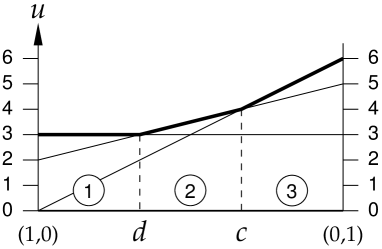
Figure 1: Upper envelope of expected payoffs to player 1, as a function of the mixed strategy $y$ of player 2, for the game (3).

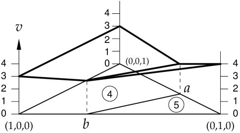
Figure 2: Perspective drawing of the upper envelope of expected payoffs to player 2, as a function of the mixed strategy $x$ of player 1, for the game (3).

We label the pure strategies of the two players uniquely by giving label $i$ to each row $i=1,\ldots,m$, and label $m+j$ to each column $j=1,\ldots,n$. In our $3\times 2$ example, the pure strategies of player 2 have therefore labels 4 and 5. Figure 2 shows the upper envelope for the two strategies of player 2 for the possible mixed strategies $x\in X$ of player 1; note that $X$ is a triangle. As found earlier in (6) and (7), for the points $a=(0,\frac{3}{5},\frac{2}{5})$ and $b=(\frac{2}{3},\frac{1}{3},0)$ in $X$ both columns have equal expected payoffs to player 2. This is also the case for any convex combination of $a$ and $b$, that is, any point on the line segment that connects $a$ and $b$. This line segment is common to the two best-response regions that otherwise partition $X$, namely the best-response region for the first column (with label 4) that is the convex hull of the points $(1,0,0)$, $b$, $a$, and $(0,0,1)$, and the best-response region for the second column (with label 5) which is the convex hull of the points $(0,1,0)$, $a$, and $b$. Both regions are shown in Figure 2.

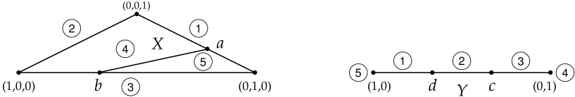
Figure 3: The mixed strategy sets $X$ and $Y$ with labels of pure best responses of the other player, and own labels where a pure strategy has probability zero.

The two strategy sets $X$ and $Y$ with their subdivision into best-response regions for the pure strategies of the other player are now given additional labels at their boundaries. Namely, a point $x$ in $X$ gets label $i$ in $\{1,\ldots,m\}$ if $x_{i}=0$, and a point $y$ in $X$ gets label $m+j$ in $\{m+1,\ldots,m+n\}$ if $y_{j}=0$. That is, the “outside labels” correspond to a player’s own pure strategies that are played with probability zero. Figure 3 shows this for the example (3). A point may have several labels of a player, if it has multiple best responses or more than one own strategy that has probability zero. For example, $x=(1,0,0)$ has the three labels $2,3,4$. The points in $X$ that have three labels, and the points in $Y$ that have two labels, are marked as dots in Figure 3. Apart from the unit vectors that are the vertices (corners) of $X$ and $Y$, these are the points $a$ and $b$ in $X$ and $c$ and $d$ in $Y$. With these labels, an equilibrium is any completely labeled pair $(x,y)$, that is, every label in $\{1,\ldots,m+n\}$ is a label of $x$ or of $y$, as the next proposition asserts.

Proposition 5.

Let $(x,y)\in X\times Y$ for an $m\times n$ bimatrix game $(A,B)$. Then $(x,y)$ is a Nash equilibrium of $(A,B)$ if and only if $(x,y)$ is completely labeled.

Proof. A missing label would represent a pure strategy of either player that is not a pure best response but has positive probability, which is exactly what is not allowed in an equilibrium according to Proposition 1.     

The advantage of this condition is that it is purely combinatorial and just depends on the labels but not on the exact position of the dots in the diagrams in Figure 3. There, because a completely labeled pair $(x,y)$ requires all five labels, three of these must be labels of $x$ and two must be labels of $y$, so it suffices to consider the finitely many points with these properties. In $Y$, there are only four points $y$ that have two labels. The first is $(1,0)$, which has labels 1 and 5. There is indeed a point in $X$ which has the other labels 2, 3, 4, namely $(1,0,0)$, so $((1,0,0),(1,0))$ is an equilibrium. Point $d=(\frac{2}{3},\frac{1}{3})$ in $Y$ has labels 1 and 2, and point $b$ in $X$ has the other labels 3, 4, 5, so $(b,d)$ is another equilibrium, in agreement with (7). Point $c=(\frac{1}{3},\frac{2}{3})$ in $Y$ has labels 2 and 3, and point $a$ in $X$ has the other labels 1, 4, 5, so $(a,b)$ is a third equilibrium, in agreement with (6). Finally, point $(0,1)$ in $Y$ has labels 3 and 4, but there is no point in $X$ that has the remaining labels 1, 2, 5, so there is no equilibrium where player 2 plays $(0,1)$. This suffices to identify all equilibria. (The remaining points $(0,1,0)$ and $(0,0,1)$ of $X$ have three labels, neither of which have corresponding points in $Y$ that have the other two labels.)

In the above example, no point in $X$ has more than three labels, and no point in $Y$ has more than two labels. In general, this is equivalent to the nondegeneracy of the game.

Proposition 6.

An $m\times n$ bimatrix game is nondegenerate if and only if no $x$ in $X$ has more than $m$ labels, and no $y$ in $Y$ has more than $n$ labels.

Proof. Let $x\in X$. The labels of $x$ are the $|\textup{\small{bestresp}}(x)|$ pure best responses to $x$ and player 1’s own strategies $i$ where $x_{i}=0$, where the number of the latter is $m-|\textup{\small{supp}}(x)|$. So if the game is degenerate because $|\textup{\small{bestresp}}(x)|>|\textup{\small{supp}}(x)|$, this is equivalent to $|\textup{\small{bestresp}}(x)|+m-|\textup{\small{supp}}(x)|>m$, that is, $x$ having more than $m$ labels. Similarly, $y$ in $Y$ has more that $|\textup{\small{supp}}(y)|$ pure best responses if and only if $y$ has more than $n$ labels. If this is never the case, the game is nondegenerate.     

We need further concepts about polyhedra and polytopes. A polyhedron $P$ in ${\mathbb{R}}^{d}$ is a set $\{z\in{\mathbb{R}}^{d}\mid Cz\leq q\}$ for some matrix $C$ and vector $q$. It is called full-dimensional if it has dimension $d$. It is called a polytope if it is bounded. A face of $P$ is a set $\{\,z\in P\mid c^{\top}z=q_{0}\}$ for some $c\in{\mathbb{R}}^{d}$ and $q_{0}\in{\mathbb{R}}$ so that the inequality $c^{\top}z\leq q_{0}$ is valid for $P$, that is, holds for all $z$ in $P$. A vertex of $P$ is the unique element of a 0-dimensional face of $P$. An edge of $P$ is a one-dimensional face of $P$. A facet of a $d$-dimensional polyhedron $P$ is a face of dimension ${d-1}$. It can be shown that any nonempty face $F$ of $P$ can be obtained by turning some of the inequalities that define $P$ into equalities, which are then called binding inequalities. That is, $F=\{\,z\in P\mid c_{i}^{\kern-0.27995pt\top\kern-0.70004pt}z=q_{i}\,,~{}i\in I\}$, where $c_{i}^{\kern-0.27995pt\top\kern-0.70004pt}z\leq q_{i}$ for $i\in I$ are some of the rows in $Cz\leq q$. A facet is characterized by a single binding inequality $c_{i}^{\kern-0.27995pt\top\kern-0.70004pt}z\leq q_{i}$ which is irredundant, that is (after omitting any equivalent inequality), the inequality cannot be omitted without changing the polyhedron; the vector $c_{i}$ is called the normal vector of the facet. A $d$-dimensional polyhedron $P$ is called simple if no point belongs to more than $d$ facets of $P$, which is true if there are no special dependencies between the facet-defining inequalities.

The subdivision of $X$ and $Y$ into best-response regions as shown in the example in Figure 3 can be nicely visualized for small games with up to four strategies per player, because then $X$ and $Y$ have dimension at most three. If the payoff matrix $A$ in the game $(A,B)$ has rows $a_{1},\ldots,a_{m}$, then the best-response region for player 1’s strategy $i$ is the set $\{y\in Y\mid a_{i}y\geq a_{k}y,~{}k=1,\ldots,m\}$ , which is a polytope since $Y$ is bounded. However, for general $m\times n$ games, the subdivision of $Y$ and $X$ into best-response regions has more structure by taking into account, as an additional dimension, the payoffs $u$ and $v$ to player 1 and 2. In Figure 2, the upper envelope of expected payoffs to player 1 is obtained by the smallest $u$ for the points $(y,u)$ in $Y\times\mathbb{R}$ so that $3y_{1}+3y_{2}\leq u$, $2y_{1}+5y_{2}\leq u$, $0y_{1}+6y_{2}\leq u$, or in general $Ay\leq\textup{{1}}u$. Similarly, Figure 2 shows the smallest $v$ for $(x,v)$ in $X\times\mathbb{R}$ with $3x_{1}+2x_{2}+3x_{3}\leq v$ and $2x_{1}+4x_{2}+0x_{3}\leq v$, or in general $B^{\kern-0.27995pt\top\kern-0.70004pt}x\leq\textup{{1}}v$. The best-response polyhedron of a player is the set of that player’s mixed strategies together with the upper envelope of expected payoffs (and any larger payoffs) to the other player. The best-response polyhedra $\overline{P}$ and $\overline{Q}$ of players 1 and 2 are therefore

$$\begin{array}[]{rll}\overline{P}&{}=\{(x,v)\in{\mathbb{R}}^{m}\times{\mathbb{R}}&{}\mid x\geq\hbox{\bf 0},~{}\hbox{\bf 1}^{\top}x=1,~{}B^{\top}x\leq\hbox{\bf 1}v\,\},\\ \overline{Q}&{}=\{(y,u)\in{\mathbb{R}}^{n}\times{\mathbb{R}}&{}\mid Ay\leq\hbox{\bf 1}u,~{}y\geq\hbox{\bf 0},~{}\hbox{\bf 1}^{\top}y=1\,\}\,.\\ \end{array}$$ (8)

Both polyhedra are defined by $m+n$ inequalities (and one additional equation). Whenever one of these inequalities is binding, we give it the corresponding label in $\{1,\ldots,m+n\}$. For example, if in the example (3) the inequality $3x_{1}+2x_{2}+3x_{3}\leq v$ of $\overline{P}$ is binding, that is, $3x_{1}+2x_{2}+3x_{3}=v$, this means that the first pure strategy of player 2, which has label 4, is a best response. The best-response region with label 4 is therefore the facet of $\overline{P}$ for this binding inequality, projected to the mixed strategy set $X$ by ignoring the payoff $v$ to player 2, as seen in Figure 2. Facets of polyhedra are easier to deal with than subdivisions of mixed-strategy simplices into best-response regions.

The binding inequalities of any $(x,v)$ in $\overline{P}$ and $(y,u)$ in $\overline{Q}$ define labels as before, so that equilibria $(x,y)$ are again identified as completely labeled pairs in $X\times Y$. The corresponding payoffs $v$ and $u$ are then on the respective upper envelope (that is, smallest), for the following reason: For any $x$ in $X$, at least one component $x_{i}$ of $x$ is nonzero, so in an equilibrium label $i$ must appear as a best response to $y$, which means that the $i$th inequality in $Ay\leq\textup{{1}}u$ is binding, that is, $(Ay)_{i}=u$, so $u$ is on the upper envelope of expected payoffs in $\overline{Q}$ as claimed; the analogous statement holds for any nonzero component $y_{j}$ of $y$ with label $m+j$.

The polyhedra $\overline{P}$ and $\overline{Q}$ in (8) can be simplified by eliminating the payoff variables $u$ and $v$, by defining the following polyhedra:

$$\begin{array}[]{rllrlrl}P&{}=\{\,x\in{\mathbb{R}}^{m}&{}\mid{}&x&{}\geq\hbox{\bf 0},{}&B^{\top}x&{}\leq\hbox{\bf 1}\},\\ Q&{}=\{\,y\in{\mathbb{R}}^{n}&{}\mid{}&Ay&{}\leq\hbox{\bf 1},{}&y&{}\geq\bf 0\}\,.\end{array}$$ (9)

We want $P$ and $Q$ to be polytopes, which is equivalent to $v>0$ and $u>0$ for any $(x,v)\in\overline{P}$ and $(y,u)\in\overline{Q}$, according to the following proposition.

Proposition 7.

Consider a bimatrix game $(A,B)$. Then $P$ in $(\ref{defPQ})$ is a polytope if and only if the best-response payoff to any $x$ in $X$ is always positive, and $Q$ in $(\ref{defPQ})$ is a polytope if and only if the best-response payoff to any $y$ in $Y$ is always positive.

Proof. We prove the statement for $Q$; the proof for $P$ is analogous. The best-response payoff to any mixed strategy $y$ is the maximum entry of $Ay$, so this is not always positive if and only if $Ay\leq\textup{{0}}$ for some $y\in Y$. For such a $y$ we have $y\geq 0$, $y\neq\textup{{0}}$, and $y\alpha\in Q$ for any $\alpha\geq 0$, which shows that $Q$ is not bounded. Conversely, suppose the best-response payoff $u$ to any $y$ is always positive. Because $Y$ is compact and $\overline{Q}$ is closed, the minimum $u^{\prime}$ of $\{u\mid\exists y~{}:~{}(y,u)\in\overline{Q}\}$ exists, $u^{\prime}>0$, and $u\geq u^{\prime}$ for all $(y,u)$ in $\overline{Q}$. Then the map

$$\overline{Q}\to Q-\{\textup{{0}}\},\qquad(y,u)\mapsto y\cdot\textstyle\frac{1}{u}$$ (10)

is a bijection with inverse $z\mapsto(z\cdot\frac{1}{\textup{{1}}^{\kern-0.19997pt\top\kern-0.50003pt}z}),\frac{1}{\textup{{1}}^{\kern-0.19997pt\top\kern-0.50003pt}z})$ for $z\in Q-\{\textup{{0}}\}$. Here, $\frac{1}{\textup{{1}}^{\kern-0.19997pt\top\kern-0.50003pt}z}\geq u^{\prime}$ and thus $\textup{{1}}^{\kern-0.27995pt\top\kern-0.70004pt}z\leq 1/u^{\prime}$, where $\textup{{1}}^{\kern-0.27995pt\top\kern-0.70004pt}z$ is the 1-norm $\sum_{j=1}^{n}|z_{j}|$ of $z$ (because $z\geq\textup{{0}}$), which proves that $Q$ is bounded and therefore a polytope.     

As a sufficient condition that $v>0$ and $u>0$ for any $(x,v)$ in $\overline{P}$ and $(y,u)$ in $\overline{Q}$, we assume that

$$A B^{\top}$$ and are nonnegative and have no zero column (11)

(because then $B^{\kern-0.27995pt\top\kern-0.70004pt}x$ and $Ay$ are nonnegative and nonzero for any $x\in X$, ${y\in Y}$). We could simply assume $A>\bf 0$ and $B>\bf 0$, but it is useful to admit zero matrix entries (e.g. as in the identity matrix). Note that condition (11) is not necessary for positive best-response payoffs (which is still the case, for example, if the zero entry of $A$ in (3) is negative, as Figure 1 shows). By adding a suitable positive constant to all payoffs of a player, which preserves the preferences of that player, we can assume (11) without loss of generality.

With positive best-response payoffs, the polytope $P$ is obtained from $\overline{P}$ by dividing each inequality $\sum_{i=1}^{m}b_{ij}x_{i}\leq v$ by $v$, which gives $\sum_{i=1}^{m}b_{ij}(x_{i}/v)\leq 1$, and then treating $x_{i}/v$ as a new variable that is again called $x_{i}$ in $P$. Similarly, $\overline{Q}$ is replaced by $Q$ by dividing each inequality in $Ay\leq\textup{{1}}u$ by $u$. In effect, we have normalized the expected payoffs on the upper envelope to be 1, and dropped the conditions $\textup{{1}}^{\top}x=1$ and $\textup{{1}}^{\top}y=1$ (so that $P$ and $Q$ have full dimension, unlike $\overline{P}$ and $\overline{Q}$). Conversely, nonzero vectors $x\in P$ and $y\in Q$ are multiplied by $v=1/\textup{{1}}^{\kern-0.27995pt\top\kern-0.70004pt}x$ and $u=1/\textup{{1}}^{\kern-0.27995pt\top\kern-0.70004pt}y$ to turn them into probability vectors. The scaling factors $v$ and $u$ are the expected payoffs to the other player.

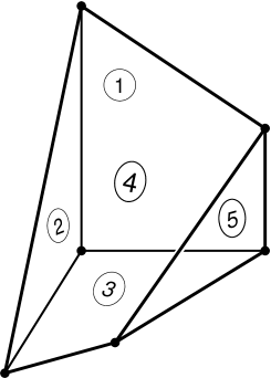
Figure 4: The polytopes $P$ and $Q$ in (9) for the game (3). Vertices are shown as dots, and facet labels as circled numbers.

Similar to (10), the set $\overline{P}$ is in one-to-one correspondence with $P-\{\textup{{0}}\}$ with the map

$$\overline{P}\to P-\{\textup{{0}}\},\qquad(x,v)\mapsto x\cdot(1/v).$$ (12)

These bijections are not linear, but are known as “projective transformations” (for a visualization see von Stengel (2002, Fig. 2.5)). They map lines to lines, and any binding inequality in $\overline{P}$ (respectively, $\overline{Q}$) corresponds to a binding inequality in $P$ (respectively, $Q$) and vice versa. Therefore, corresponding points have the same labels defined by the binding inequalities, which are some of the $m+n$ inequalities that define $P$ and $Q$ in (9), see Figure 4. An equilibrium is then a (re-scaled) completely labeled pair $(x,y)\in P\times Q-\{(\textup{{0}},\textup{{0}})\}$ that has for each label $i$ the respective binding $i$th inequality in $x\geq\textup{{0}}$ or $Ay\leq\textup{{1}}$, and for each label $m+j$ the respective binding $j$th inequality in $B^{\kern-0.27995pt\top\kern-0.70004pt}x\leq\textup{{1}}$ or $y\geq\textup{{0}}$.

With assumption (11) and the polytopes $P$ and $Q$ in (9), an improved algorithm compared to Algorithm 4 is to find all completely labeled vertex pairs $(x,y)$ of $P\times Q$. A simple example of the resulting improvement is an $m\times 2$ game where $\overline{Q}$, similar to Figure 1, has at most $m+1$ vertices, as opposed to about $m^{2}/2$ supports of size at most two for player 1. For square games where $m=n$, the maximum number of support pairs versus vertices to be tested changes from about $4^{n}$ to about $2.6^{n}$ (Keiding, 1997; von Stengel, 2002, p. 1724). We will describe an algorithm that finds all equilibria, even in a degenerate game, in Section 9. Before that, we will describe a classic algorithm that finds at least one Nash equilibrium of a bimatrix game, which also proves that a Nash equilibrium exists.

4   The Lemke-Howson algorithm

Lemke and Howson (1964) (LH) described an algorithm that finds one Nash equilibrium of a bimatrix game. It proves the existence of a Nash equilibrium for nondegenerate games, which can also be adapted to degenerate games. We first explain this algorithm following Shapley (1974). In the next section we describe it using the polytopes from the previous Section 3.

Consider a nondegenerate bimatrix game and Figure 3 for the example (3). The mixed-strategy simplices $X$ and $Y$ are subdivided into best-response regions which are labeled with the other player’s best responses, and the facets of the simplices are labeled with the unplayed own pure strategies. These labels give rise to a graph that consists of finitely many vertices, joined by edges. A vertex is any point of $X$ that has $m$ labels. An edge of the graph for $X$ is a set of points defined by $m-1$ labels. Its endpoints are the two vertices that have these ${m-1}$ labels in common; for example, the vertices $a$ and $b$ are joined by the edge with labels 4 and 5. As shown in Theorem 14(g) below, nondegeneracy implies that the faces of $P$ that are defined by $m$ and $m-1$ labels are indeed vertices and edges of $P$, which correspond to these graph vertices and edges. There are only finitely many sets with $m$ labels and therefore only finitely many vertices. Similarly, every vertex and edge of $Y$ is defined by $n$ and ${n-1}$ labels, respectively.

We now extend the graph for $X$ by adding another vertex 0 in $\mathbb{R}^{m}$ to obtain an extended graph $\tilde{X}$. The new vertex 0 has all labels $1,\ldots,m$, and is connected by an edge to each unit vector $e_{i}$ (which is a vertex of $X$), which has all labels $1,\ldots,m$ except $i$. One can also consider $\tilde{X}$ geometrically as the convex hull of $X$ and 0. This is an $m$-dimensional simplex in $\mathbb{R}^{m}$ with $X$ as one facet (subdivided and labeled as before) and $m$ additional facets $\{x\in\tilde{X}\mid x_{i}=0\}$ for each $i=1,\ldots,m$, with label $i$, which produces the described labels. However, only the graph structure of $\tilde{X}$ matters. In the same way, $Y$ is extended to $\tilde{Y}$ with an extra vertex 0 in $\mathbb{R}^{n}$ that has all labels $m+1,\ldots,m+n$, which is connected by $n$ edges to the $n$ unit vectors in $Y$. The extended graphs $\tilde{X}$ and $\tilde{Y}$ are shown in Figure 5.

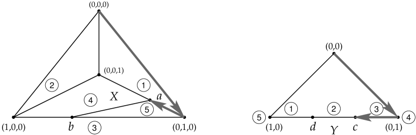
Figure 5: Extension $\tilde{X}$ of $X$ and $\tilde{Y}$ of $Y$, each with an additional vertex 0. The artificial equilibrium $(\textup{{0}},\textup{{0}})$ is completely labeled. The arrows show the LH (Lemke-Howson) path starting from $(\textup{{0}},\textup{{0}})$ for missing label 2.

The point $(\textup{{0}},\textup{{0}})$ of $\tilde{X}\times\tilde{Y}$ is completely labeled, but does not represent a mixed strategy pair. We call it the artificial equilibrium, which is the starting point of the LH algorithm. For the algorithm, one label $k$ in $\{1,\ldots,m,m+1,\ldots,m+n\}$ is declared as possibly missing. The algorithm computes a path in $\tilde{X}\times\tilde{Y}$, which we first describe for our example and then in general.

Figure 5 shows the LH path for missing label 2. The starting point is $(x,y)=((0,0,0),(0,0))$, where $x$ has labels $1,2,3$ and $y$ has labels $4,5$. With label 2 allowed to be missing, we start by dropping label 2, which means changing $x$ along the unique edge that connects $(0,0,0)$ to $(0,1,0)$ (shown by an arrow in the figure), while keeping $y=(0,0)$ fixed. The endpoint $x=(0,1,0)$ of that arrow has a new label 5 which is picked up. Because $x$ has three labels $1,3,5$ and $y=(0,0)$ has two labels $4,5$ but label 2 is missing, the label 5 that has just been picked up in $\tilde{X}$ is now duplicate. Because $y$ no longer needs to have the duplicate label 5, the next step is to drop label 5 in $\tilde{Y}$, that is, change $y$ from $(0,0)$ to $(0,1)$ along the edge which has only label 4. At the end of that edge, $y=(0,1)$ has labels 4 and 3, where label 3 has been picked up. The current point $(x,y)=((0,1,0),(0,1))$ therefore has duplicate label 3. Correspondingly, we can now drop label 3 in $\tilde{X}$, that is, move $x$ along the edge with labels 1 and 5 to point $a$, where label 4 is picked up. At the current point $(x,y)=(a,(0,1))$, label 4 is duplicate. Next, we drop label 4 in $\tilde{Y}$ by moving $y$ along the edge with label 3 to reach point $c$, where label 2 is picked up. Because 2 is the missing label, the reached point $(x,y)=(a,c)$ is completely labeled. This is the equilibrium that is found as the endpoint of the LH path.

In general, the algorithm traces a path that consists of points $(x,y)$ in $\tilde{X}\times\tilde{Y}$ that have all labels except possibly label $k$. Because $(x,y)$ has at least $m+n-1$ labels, this is only possible in the following cases. Suppose $x$ is a vertex of $\tilde{X}$ (which has $m$ labels) and $y$ is a vertex of $\tilde{Y}$ (which has $n$ labels). If $(x,y)$ has all labels $1,\ldots,m+n$ then it is an equilibrium. If $(x,y)$ has all labels except label $k$, then $x$ and $y$ have exactly one label in common, which is the duplicate label. Alternatively, either $x$ has $m$ labels and is therefore a vertex of $\tilde{X}$ and $y$ has $n-1$ labels and belongs to an edge of $\tilde{Y}$, or $x$ has $m-1$ labels and belongs to an edge of $\tilde{X}$ and $y$ has $n$ labels and is therefore a vertex of $\tilde{Y}$. These two possibilities $\{x\}\times F$ with $y\in F$ for an edge $F$ of $\tilde{Y}$, or $E\times\{y\}$ with $x\in E$ for an edge $E$ of $\tilde{X}$, define the edges of the product graph $\tilde{X}\times\tilde{Y}$. The vertices of this product graph are of the form $(x,y)$ where $x$ is a vertex of $\tilde{X}$ and $y$ is a vertex of $\tilde{Y}$. The LH algorithm generates a path in this product graph. The steps of the algorithm alternate between traversing an edge of $\tilde{X}$ while keeping a vertex of $\tilde{Y}$ fixed and vice versa.

The LH algorithm works because there is a unique next edge in every step, which for the start depends on the chosen missing label $k$. The algorithm starts from the artificial equilibrium $(x,y)=(\textup{{0}},\textup{{0}})$ which is completely labeled. If the missing label $k$ is in $\{1,\ldots,m\}$ then the unique start is to move $x$ along the edge in $\tilde{X}$ that connects 0 to the unit vector $e_{k}$ because this is the only edge that has all labels except $k$. If $k=m+j$ for $j$ in $\{1,\ldots,n\}$ then the unique start is to move $y$ in $\tilde{Y}$ to $e_{j}$. After that, a new label is picked which (unless it is $k$) is duplicate, and there is a unique edge in the other graph ($\tilde{Y}$ or $\tilde{X}$) where that duplicate label is dropped, to continue the path. If the label that is picked up is the missing label $k$ then the algorithm terminates at an equilibrium. This cannot be the artificial equilibrium because the edge that reaches the equilibrium would offer a second way to start, which is not the case (because any edge of $\tilde{X}\times\tilde{Y}$ that has all labels except $k$ could also be traversed in the other direction). Similarly, a vertex pair $(x,y)$ of $\tilde{X}\times\tilde{Y}$ cannot be re-visited because this would mean a second way to continue, which is also not the case. These two (excluded) possibilities are shown abstractly in Figure 6.

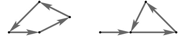
Figure 6: The LH algorithm cannot return to its starting point $(\textup{{0}},\textup{{0}})$ or re-visit an earlier vertex pair $(x,y)$ because this would imply alternative choices for starting or continuing.

The LH algorithm can be started at any equilibrium, not just the artificial equilibrium $(\textup{{0}},\textup{{0}})$. For example, in Figure 5, starting it with missing label 2 from the equilibrium $(a,c)$ that has just been found would simply traverse the path back to the artificial equilibrium. However, as shown in Figure 7, if started from the pure-strategy equilibrium $(x,y)=((1,0,0),(1,0))$ for missing label 2, it proceeds as follows: Dropping label 2 in $\tilde{X}$ changes to $(b,y)$ where label 5 is picked up. Dropping the duplicate label 5 in $\tilde{Y}$ changes to $(b,d)$ where label 2 is picked up. This is the missing label, so the algorithm finds the equilibrium $(b,d)$. This has to be a new equilibrium because $(\textup{{0}},\textup{{0}})$ and $(a,c)$ are connected by the unique LH path for missing label 2 to which there is no other access.

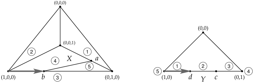
Figure 7: LH path for missing label 2 when started at the pure-strategy equilibrium $((1,0,0),(1,0))$, which leads to the equilibrium $(b,d)$.

Hence, we obtain the following important consequence.

Theorem 8.

Any nondegenerate bimatrix game has an odd number of Nash equilibria.

Proof. Fix a missing label $k$. Then the artificial equilibrium $(\textup{{0}},\textup{{0}})$ and all Nash equilibria are the unique endpoints of the LH paths for missing label $k$. The number of endpoints of these paths is even, exactly one of which is the artificial equilibrium, so the number of Nash equilibria is odd.     

The LH paths for missing label $k$ are the sets of edges and vertices of $\tilde{X}\times\tilde{Y}$ that have all labels except possibly $k$. These may also create cycles which have no endpoints. Such cycles may occur but do not affect the algorithm.

A different missing label may change how the artificial equilibrium and the Nash equilibria are “paired” as endpoints of each LH path for that missing label. For example, any pure Nash equilibrium is connected in two steps to the artificial equilibrium via a suitable missing label. Suppose the pure strategy equilibrium is $(i,j)$. Choose $k=i$ as the missing label. Then the LH path first moves in $\tilde{X}$ to $(e_{i},\textup{{0}})$ where the label that is picked up is $m+j$ because $j$ is the best response to $i$. The next step is then to $(e_{i},e_{j})$ where the algorithm terminates because the best response to $j$ is $i$ which is the missing label. In the above example in Figure 7, the pure-strategy equilibrium $((1,0,0),(1,0))$ can therefore be found via missing label 1 (or missing label 4 which corresponds to player 2’s pure equilibrium strategy). As shown earlier, missing label 2 connects the artificial equilibrium to $(a,c)$, and therefore the LH path for missing label 2 when started from $((1,0,0),(1,0))$ necessarily leads to a third equilibrium. However, the “network” obtained by connecting equilibria via LH paths for different missing labels may still not connect all Nash equilibria directly or indirectly to the artificial equilibrium. An example due to Robert Wilson has been given by Shapley (1974, Fig. 3), which is a $3\times 3$ game where for every missing label the LH path from the artificial equilibrium leads to the same Nash equilibrium, and two further Nash equilibria (which are unreachable this way) are connected to each other.

In order to run the LH algorithm, it is not necessary to create the graphs $\tilde{X}$ and $\tilde{Y}$ in full (which would directly allow finding all Nash equilibria as completely labeled vertex pairs). Rather, the alternate traversal of the edges of these graphs can be done in each step by a local “pivoting” operation that is similarly known for the simplex algorithm for linear programming. We explain this in Section 8.

5   Lemke-Howson paths on polytopes

A convenient way to implement the LH algorithm uses the polytopes $P$ and $Q$ in (9) rather than the projections of the best-response polyhedra $\overline{P}$ and $\overline{Q}$ in (8) to $X$ and $Y$. The polytopes $P$ and $Q$ have the extra point 0 which is the only point not in correspondence to the polyhedron $\overline{P}$ and $\overline{Q}$ via a projective transformation as in (10). The extra point $(\textup{{0}},\textup{{0}})\in P\times Q$ is completely labeled and represents the artificial equilibrium where the LH algorithm starts.

We now consider a more general setting. A Linear Complementarity Problem or LCP is given by a $d\times d$ matrix $C$ and a vector $q\in\mathbb{R}^{d}$, where the problem is to find $z\in\mathbb{R}^{d}$ so that

$$z\geq\textup{{0}},\qquad w=q-Cz\geq\textup{{0}},\qquad z^{\kern-0.27995pt\top\kern-0.70004pt}w=0$$ (13)

(the standard notation for an LCP, see Cottle, Pang, and Stone, 1992, uses $-M$ instead of $C$ and $n$ instead of $d$). In (13), because both $z$ and $w$ are nonnegative, the orthogonality condition $z^{\kern-0.27995pt\top\kern-0.70004pt}w=0$ is equivalent to the condition $z_{i}w_{i}=0$ for each $i=1,\ldots,d$, which means that at least one of the variables $z_{i}$ and $w_{i}$ is zero; these variables are therefore also called complementary.

A geometric way to view an LCP is the following. Consider the polyhedron $S$ in $\mathbb{R}^{d}$ given by

$$S=\{z\in\mathbb{R}^{d}\mid z\geq\textup{{0}},~{}Cz\leq q\,\}.$$ (14)

For any $z\in S$, we say $z$ has label $i$ in $\{1,\ldots,d\}$ if $z_{i}=0$ or if $(Cz)_{i}=q_{i}$, and call $z$ completely labeled if $z$ has all labels $1,\ldots,d$. Clearly, $z$ is a solution to the LCP (13) if and only if $z\in S$ and $z$ is completely labeled.

In $S$, the $2d$ inequalities $z\geq 0$, $Cz\leq q$ have the labels $1,\ldots,d,1,\ldots,d$ (which means every label occurs twice) and $z$ in $S$ has label $i$ if one of the corresponding inequalities is binding. The labels of $S$ in (14) should be thought of as labeling the facets of $S$. We assume $S$ is nondegenerate, that is, no $z\in S$ has more than $d$ binding inequalities. As shown in Theorem 14(h) below, this is equivalent to the following conditions: $S$ is a simple polytope (no point is on more than $d$ facets), and no inequality can be omitted without changing $S$, unless it is never binding. Every facet therefore corresponds to a unique binding inequality, and has the corresponding label. Any edge of $S$ is defined by $d-1$ facets, and any vertex by $d$ facets. Any point has the labels of the facets it lies on.

Consider an $m\times n$ bimatrix game $(A,B)$, which may be degenerate. Assume that $P$ and $Q$ in (9) are polytopes, if necessary by adding a constant to the payoffs (see Proposition 7). Then any Nash equilibrium of $(A,B)$ is given by a solution $z=(x,y)\in P\times Q=S$ with $z\neq\textup{{0}}$ to the LCP (13). That is, $d=m+n$ and $q=\textup{{1}}\in\mathbb{R}^{m+n}$, and

$$C=\left[\begin{matrix}0~{}~{}~{}&A\\ B^{\kern-0.27995pt\top\kern-0.70004pt}~{}~{}&0\\ \end{matrix}\,\right]$$ (15)

where $0$ is an all-zero matrix (of size $m\times m$ and $n\times n$, respectively). The $m+n$ labels are exactly as described in Section 3, and correspond to unplayed pure strategies $i$ if $z_{i}=0$ or best-response pure strategies $i$ if $(Cz)_{i}=q_{i}=1$. As before, for $z=(x,y)$ the vectors $x$ and $y$ have to be re-scaled to represent mixed strategies. Moreover, $S$ is nondegenerate if and only if the game $(A,B)$ is nondegenerate, by Proposition 6.

We now study the LH algorithm without assuming the product structure $S=P\times Q$ for $S$, which simplifies the description. Let $S$ in (14) be a nondegenerate polytope so that 0 is a vertex of $S$. By nondegeneracy, when $z=\textup{{0}}$ then the remaining $d$ inequalities $Cz\leq q$ are strict, that is, $\textup{{0}}<q$. We can therefore divide the $i$th inequality (that is, the $i$th row of $C$ and of $q$) by $q_{i}$ and thus assume $q=\textup{{1}}$. This polytope has also a game-theoretic interpretation.

Proposition 9.

Let

$$S=\{z\in\mathbb{R}^{d}\mid z\geq\textup{{0}},~{}Cz\leq\textup{{1}}\,\}$$ (16)

be a polytope with its $2d$ inequalities labeled $1,\ldots,d,1,\ldots,d$. Then $z\in S-\{\textup{{0}}\}$ is completely labeled if and only if (with $z$ re-scaled as a mixed strategy) $(z,z)$ is a symmetric Nash equilibrium of the symmetric $d\times d$ game $(C,C^{\kern-0.27995pt\top\kern-0.70004pt})$.

Proof. In the game $(C,C^{\kern-0.27995pt\top\kern-0.70004pt})$, let $y$ be a mixed strategy of player 2, where the best-response payoff $\max_{i}(Cy)_{i}$ against $y$ is always positive because $S$ is a polytope (see Proposition 7 where this is stated for $Q$ instead of $S$). Re-scaling the best-response payoff against $y$ to $1$ and re-scaling $y$ to $z$ gives the inequality $Cz\leq\textup{{1}}$, where $z\geq\textup{{0}}$. By Proposition 1, $z$ has all labels $1,\ldots,d$ if and only if $(y,y)$ is a Nash equilibrium of $(C,C^{\kern-0.27995pt\top\kern-0.70004pt})$.     

Hence, the equilibria of a bimatrix game $(A,B)$ correspond to the symmetric equilibria of the symmetric game $(C,C^{\kern-0.27995pt\top\kern-0.70004pt})$ in (15). This “symmetrization” seems to be a folklore result, first stated for zero-sum games by Gale, Kuhn, and Tucker (1950).

We now express the LH algorithm in terms of computing a path of edges of the polytope $S$.

Proposition 10.

Suppose $S$ in $(\ref{sym})$ is a nondegenerate polytope, with its $2d$ inequalities labeled $1,\ldots,d,1,\ldots,d$. Then $S$ has an even number of completely labeled vertices, including 0.

Proof. This a consequence of the LH algorithm applied to $S$. Fix a label $k$ in $\{1,\ldots,d\}$ as allowed to be missing and consider the set of all points of $S$ that have all labels except possibly $k$. This defines a set of vertices and edges of $S$, which we call the missing-$k$ vertices (which may nevertheless also have label $k$) and edges. Any missing-$k$ vertex is either completely labeled (for example, 0), or has a duplicate label, say $\ell$. A completely labeled vertex $z$ is the endpoint of a unique missing-$k$ edge which is defined by the $d-1$ facets that contain $z$ except for the facet with label $k$, by “moving away” from that facet. If the missing-$k$ vertex $z$ does not have label $k$, then it is the endpoint of two missing-$k$ edges, each obtained by moving away from one of the two facets with the duplicate label $\ell$. Hence, the missing-$k$ vertices and edges define a collection of paths and cycles, where the endpoints of the paths are the completely labeled vertices. Their total number is even because each path has two endpoints.     

For the game $(C,C^{\kern-0.27995pt\top\kern-0.70004pt})$ with

$$C=\left[\,\begin{matrix}0&3&0\\ 2&2&2\\ 4&0&0\end{matrix}\,\right],$$ (17)

the polytope $S$ in (16) is shown in Figure 8 in a suitable planar projection (where all facets are visible except for the facet defined by $z_{1}=0$ with label 1 at the back of the polytope). The diagram shows also the LH path for missing label 1. The polytope has only two completely labeled vertices, 0 and $x=(\frac{1}{6},\frac{1}{3},0)$.

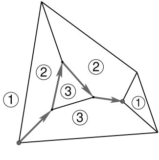
Figure 8: Left: LH path for missing label 1 for the polytope $S$ with $C$ as in (17). Right: Opposite orientation $-1$ and $+1$ of the labels $1,2,3$ around the two completely labeled vertices 0 and $x$.

6   Endpoints of LH paths have opposite index

In this section we prove a stronger version of Proposition 10. Namely, the endpoints of an LH path will be shown to have opposite “signs” $-1$ and $+1$, which are independent of the missing label. This “sign” is called the index of a Nash equilibrium, which we define here in an elementary way using determinants. By convention, the artificial equilibrium has index $-1$. This implies that every nondegenerate bimatrix game has $r$ Nash equilibria of index $+1$ and $r-1$ Nash equilibria of index $-1$, for some integer $r\geq 1$.

The right diagram in Figure 8 illustrates this concept geometrically. For a given completely labeled vertex, the index describes the orientation of the labels around the vertex. Around 0 the labels $1,2,3$ appear clockwise, which is considered a negative orientation and defines index $-1$, whereas around the Nash equilibrium $x$ they appear counterclockwise, which is a positive orientation and defines index $+1$. We can also argue geometrically that the endpoints of an LH path, here for missing label 1, have opposite index. Starting from 0, the unique edge with missing label 1 has label 2 on the left side of the path and label 3 on the right side of the path. As can be seen from the diagram, this holds for all missing-1 edges when following the path. The path terminates when it hits a facet with label 1, which is now in front of the edge of the path which has label 2 on the left and label 3 on the right, so the labels $1,2,3$ are in opposite orientation to the starting point where label 1 is behind the edge of the path. In addition, the LH path has a well-defined local direction that indicates where to go “forward” in order to reach the endpoint with index $+1$, even if one does not remember where one started: The forward direction has label 2 on the left and label 3 on the right.

We show these properties of the index for labeled polytopes $S$ as in Proposition 10 for general dimension $d$. Our argument substantially simplifies the proof by Shapley (1974) who first defined the index for Nash equilibria of bimatrix games.

Definition 11.

Consider a labeled nondegenerate polytope

$$\{z\in{\mathbb{R}}^{d}\mid{c_{j}^{\kern-0.27995pt\top\kern-0.70004pt}z\leq q_{j}}\hbox{ for }j=1,\ldots,N\}$$ (18)

where each inequality $c_{j}^{\kern-0.27995pt\top\kern-0.70004pt}z\leq q_{j}$ for $j=1,\ldots,N$ has some label in $\{1,\ldots,d\}$. Consider a completely labeled vertex $x$ of $S$ where $\lambda(i)$ indicates the inequality $c_{\lambda(i)}^{\kern-0.27995pt\top\kern-0.70004pt}x=q_{\lambda(i)}$ that is binding for $x$ and has label $i$, for $i=1,\ldots,d$. Then the index of $x$ is defined as the sign of the following determinant (multiplied by $-1$ if $d$ is even):

$$(-1)^{d+1}\,\textup{\small{sign}}|c_{\lambda(1)}\cdots c_{\lambda(d)}|.$$ (19)

A $d\times d$ matrix formed by $d$ linearly independent vectors in $\mathbb{R}^{d}$ has a nonzero determinant, but its sign is only well defined for a specific order of these vectors. For a vertex of a nondegenerate polytope as in (18), the normal vectors $c_{j}$ of its binding inequalities are linearly independent (see Theorem 14(e) below). When the vertex is completely labeled, we write down these normal vectors in the order of their labels, that is, for $j=\lambda(i)$ for $i=1,\ldots,d$, and consider the resulting $d\times d$ determinant in (19). The sign correction for even dimension $d$ is made for the following reason. For the polytope $S$ in (16) we write $z\geq\textup{{0}}$ as $-z\leq\textup{{0}}$ so all inequalities go in the same direction as required in (18). For the completely labeled vertex 0 we thus obtain the determinant of the negative of the $d\times d$ identity matrix, which is $1$ if $d$ is even and $-1$ if $d$ is odd. In order to obtain a negative index for this artificial equilibrium, we therefore multiply the sign of the determinant with $(-1)^{d+1}$.

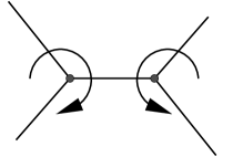
Figure 9: Opposite geometric orientation of adjacent vertices $x$ and $y$ as in Lemma 12 for $d=3$. The four involved facets are shown with their normal vectors.

The next lemma states that “pivoting changes sign” in the following sense. “Pivoting” is the algebraic representation of moving from a vertex to an “adjacent” vertex along an edge. This means that one binding inequality is replaced by another. For any fixed order of the normal vectors of the binding inequalities, one of these vectors is thus replaced by another, which we choose to be the vector in first position. The lemma states that the corresponding determinants then have opposite sign; it is geometrically illustrated in Figure 9.

Lemma 12.

Consider a nondegenerate polytope $S$ as in $(\ref{Sine})$, and an edge defined by $d-1$ binding inequalities $c_{\lambda(i)}^{\kern-0.27995pt\top\kern-0.70004pt}\,z=q_{\lambda(i)}$ for $i=2,\ldots,d$. Let $x$ and $y$ be the endpoints of this edge, with the additional binding inequality $c_{\lambda(1)}^{\kern-0.27995pt\top\kern-0.70004pt}\,x=q_{\lambda(1)}$ for $x$ and $c_{\lambda(0)}^{\kern-0.27995pt\top\kern-0.70004pt}\,y=q_{\lambda(0)}$ for $y$. Then

$$\textup{\small{sign}}|c_{\lambda(1)}c_{\lambda(2)}\ldots c_{\lambda(d)}|=-\textup{\small{sign}}|c_{\lambda(0)}c_{\lambda(2)}\ldots c_{\lambda(d)}|\neq 0.$$ (20)

Proof. Because $S$ is nondegenerate, $x$ and $y$ have exactly $d$ binding inequalities, so that the following conditions hold:

$$\begin{array}[]{rclrcl}c_{\lambda(0)}^{\kern-0.27995pt\top\kern-0.70004pt}\,x&<&q_{\lambda(0)}~{},&\qquad c_{\lambda(0)}^{\kern-0.27995pt\top\kern-0.70004pt}\,y&=&q_{\lambda(0)}~{},\\ c_{\lambda(1)}^{\kern-0.27995pt\top\kern-0.70004pt}\,x&=&q_{\lambda(1)}~{},&\qquad c_{\lambda(1)}^{\kern-0.27995pt\top\kern-0.70004pt}\,y&<&q_{\lambda(1)}~{},\\ c_{\lambda(2)}^{\kern-0.27995pt\top\kern-0.70004pt}\,x&=&q_{\lambda(2)}~{},&\qquad c_{\lambda(2)}^{\kern-0.27995pt\top\kern-0.70004pt}\,y&=&q_{\lambda(2)}~{},\\ &\vdots&&&\vdots&\\ c_{\lambda(d)}^{\kern-0.27995pt\top\kern-0.70004pt}\,x&=&q_{\lambda(d)}~{},&\qquad c_{\lambda(d)}^{\kern-0.27995pt\top\kern-0.70004pt}\,y&=&q_{\lambda(d)}~{}.\\ \end{array}$$ (21)

The $d+1$ vectors $c_{\lambda(0)},c_{\lambda(1)},\ldots,c_{\lambda(d)}$ are linearly dependent, so there are reals $\gamma_{0},\gamma_{1},\ldots,\gamma_{d}$, not all zero, with

$$\gamma_{0}\,c_{\lambda(0)}^{\kern-0.27995pt\top\kern-0.70004pt}+\gamma_{1}\,c_{\lambda(1)}^{\kern-0.27995pt\top\kern-0.70004pt}+\cdots+\gamma_{d}\,c_{\lambda(d)}^{\kern-0.27995pt\top\kern-0.70004pt}=\textup{{0}}^{\kern-0.27995pt\top\kern-0.70004pt}$$ (22)

where $\gamma_{0}\neq 0$ and $\gamma_{1}\neq 0$ because otherwise the binding inequalities for $x$ or $y$ would be linearly dependent, which is not the case. Hence, by (22) and (21),

$$0=\textup{{0}}^{\kern-0.27995pt\top\kern-0.70004pt}(y-x)=\gamma_{0}\,c_{\lambda(0)}^{\kern-0.27995pt\top\kern-0.70004pt}(y-x)+\gamma_{1}\,c_{\lambda(1)}^{\kern-0.27995pt\top\kern-0.70004pt}(y-x)$$

and therefore

$$\frac{\gamma_{0}}{\gamma_{1}}~{}=~{}\frac{c_{\lambda(1)}^{\kern-0.27995pt\top\kern-0.70004pt}\,x-c_{\lambda(1)}^{\kern-0.27995pt\top\kern-0.70004pt}\,y}{c_{\lambda(0)}^{\kern-0.27995pt\top\kern-0.70004pt}\,y-c_{\lambda(0)}^{\kern-0.27995pt\top\kern-0.70004pt}\,x}~{}>~{}0$$ (23)

by the first two rows in (21). The linear dependence (22) and multilinearity of the determinant imply

$$\begin{array}[]{rcl}0&=&|(c_{\lambda(0)}\gamma_{0}+c_{\lambda(1)}\gamma_{1})~{}c_{\lambda(2)}\cdots c_{\lambda(d)}|\\ &=&|c_{\lambda(0)}~{}c_{\lambda(2)}\cdots c_{\lambda(d)}|\,\gamma_{0}~{}+~{}|c_{\lambda(1)}~{}c_{\lambda(2)}\cdots c_{\lambda(d)}|\,\gamma_{1}\\ \end{array}$$ (24)

and thus

$$|c_{\lambda(1)}~{}c_{\lambda(2)}\cdots c_{\lambda(d)}|~{}=~{}-|c_{\lambda(0)}~{}c_{\lambda(2)}\cdots c_{\lambda(d)}|\frac{\gamma_{0}}{\gamma_{1}}$$ (25)

which shows (20).     

Theorem 13.

Suppose $S$ in $(\ref{sym})$ is a nondegenerate polytope, with its $2d$ inequalities labeled $1,\ldots,d,1,\ldots,d$. Then $S$ has an even number of completely labeled vertices. Half of these (including 0) have index $-1$, the other half index $+1$. The endpoints of any LH path have opposite index.

Proof. Let $S$ be described as in (18), so that $c_{i}=-e_{i}$ for $i=1,\ldots,d$ and $C^{\kern-0.27995pt\top\kern-0.70004pt}=[c_{d+1}\cdots c_{2d}]$. Consider some completely labeled vertex $x$ of $S$. Let the binding inequalities for $x$ be $c_{\lambda(i)}^{\kern-0.27995pt\top\kern-0.70004pt}\,x=q_{i}$ with label $i$ for $i=1,\ldots,d$. We consider the LH path with missing label 1 that starts at $x$, and show that the endpoint of that path has opposite index to $x$. Suppose that $x$ has negative index and that $d$ is odd, so that $|c_{\lambda(1)}~{}c_{\lambda(2)}\cdots c_{\lambda(d)}|<0$. On the first edge of the LH path with missing label 1, the same inequalities as for $x$ are binding, except for the inequality $c_{\lambda(1)}^{\kern-0.27995pt\top\kern-0.70004pt}\,z\leq q_{1}$. Let the endpoint of that edge be $y$, where now the inequality $c_{\lambda(0)}^{\kern-0.27995pt\top\kern-0.70004pt}\,y\leq q_{0}$ is binding. This is the situation of Lemma 12, so $|c_{\lambda(0)}~{}c_{\lambda(2)}\cdots c_{\lambda(d)}|>0$ by (20). If the binding inequality $c_{\lambda(1)}^{\kern-0.27995pt\top\kern-0.70004pt}\,y\leq q_{1}$ has the missing label 1, the claim is proved, because then $y$ is the other endpoint of the LH path, and has positive index.

So suppose this is not the case, that is, the binding inequality $c_{\lambda(1)}^{\kern-0.27995pt\top\kern-0.70004pt}\,y\leq q_{1}$ has a duplicate label $\ell$ in $\{2,\ldots,d\}$. We now exchange columns $1$ and $\ell$ in the matrix $[c_{\lambda(0)}~{}c_{\lambda(2)}\cdots c_{\lambda(d)}]$, which changes the sign of its determinant, which is now

$$|c_{\lambda(\ell)}~{}c_{\lambda(2)}\cdots c_{\lambda(\ell-1)}~{}c_{\lambda(0)}~{}c_{\lambda(\ell+1)}\cdots c_{\lambda(d)}|$$ (26)

and again negative. Note that these are still the same normal vectors of the binding inequalities for $y$, except for the exchanged columns $1$ and $\ell$; moreover, columns $2,\ldots,d$ have labels $2,\ldots,d$ in that order. The first column in (26) has the duplicate label $\ell$, and corresponds to the inequality $c_{\lambda(\ell)}^{\kern-0.27995pt\top\kern-0.70004pt}\,y\leq q_{\ell}$ that is no longer binding when label $\ell$ is dropped for the next edge on the LH path. That is, (26) represents the same situation as the starting point $x$ : The determinant is negative, columns $2,\ldots,d$ have the correct labels, and the first column will be exchanged for a new column when traversing the next edge. The resulting determinant with the new first column has opposite sign by Lemma 12. If the label that has been picked up is the missing label 1, then it is the endpoint of the LH path and the claim is proved. Otherwise we again exchange the first column with the column of the duplicate label, with the determinant going back to negative, and repeat, until the endpoint of the path is reached.

On any missing-1 vertex on the path, we also can identify the direction of the path by considering the two determinants obtained by exchanging the first column and the column with its duplicate label (in both cases, columns $2,\ldots,d$ have the correct labels). The pivoting step (which determines the edge to be traversed) replaces the first column of the determinant. If it starts from a negative determinant, then the direction is towards the endpoint with positive index (for odd $d$, as in our description so far). If it starts from a positive determinant, then the direction is towards the endpoint with negative index.

Clearly, the analogous reasoning applies if the considered starting point $x$ of the LH path has positive index or if $d$ is even. Because the endpoints of the LH paths for missing label 1 have opposite index, half of these endpoints have index $-1$ and the other half index $+1$, as claimed.

As concerns missing labels $k$ other than label 1, we can reduce this to the case $k=1$ as follows: We exchange the first and $k$th coordinate of $\mathbb{R}^{d}$ as the ambient space of $S$, and the first and $k$th row in the $d$ inequalities $-z\leq\textup{{0}}$ as well as in $Cz\leq\textup{{1}}$. This double exchange of rows and columns does not change the signs of the determinant (19) of any completely labeled vertex, and the LH path for missing label $k$ becomes the LH path for missing label 1 where the preceding reasoning applies.     

$$\begin{array}[]{rrrrl c rrrrl}&&-1&&&&&&+1&&\\ |&-e_{1}&-e_{2}&-e_{3}&|&~{}~{}\includegraphics[width=34.1433pt]{FIG/arrow.pdf}{}{}&|&c_{3}&-e_{2}&-e_{3}&|\\ |&-e_{3}&-e_{2}&c_{3}&|&\includegraphics[width=34.1433pt]{FIG/2arrow.pdf}&|&c_{2}&-e_{2}&c_{3}&|\\ |&-e_{2}&c_{2}&c_{3}&|&\includegraphics[width=34.1433pt]{FIG/2arrow.pdf}&|&-e_{3}&c_{2}&c_{3}&|\\ |&c_{3}&c_{2}&-e_{3}&|&\includegraphics[width=34.1433pt]{FIG/2arrow.pdf}&|&c_{1}&c_{2}&-e_{3}&|\\ \end{array}$$

Figure 10: Illustration of the proof of Theorem 13 with facets of $S$ in (16) shown by their normal vectors (whose subscripts are their labels), which are either the negative unit vectors $-e_{1}$, $-e_{2}$, $-e_{3}$, or $c_{1}^{\kern-0.25195pt\top\kern-0.63004pt}$, $c_{2}^{\kern-0.25195pt\top\kern-0.63004pt}$, $c_{3}^{\kern-0.25195pt\top\kern-0.63004pt}$ as the three rows of the matrix $C$ in (17).

Figure 10 illustrates the proof of Theorem 13 where the right-hand side shows two columns that display the determinants with sign $-1$ and $+1$ for the steps of the algorithm. It starts at the completely labeled vertex 0, which has the negative unit vectors as normal vectors of its binding inequalities. Dropping label 1 and picking up label 3 exchanges $-e_{1}$ with $c_{3}$, with the sign of the determinant changed from $-1$ to $+1$. This is the edge from 0 to $y$. The double-headed arrow shows the switch to the next line which exchanges the columns $c_{3}$ and $-e_{3}$ with the duplicate label 3, and brings the determinant back to $-1$, but still refers to the same point $y$. The next step away from $y$ exchanges the column $-e_{3}$ with $c_{2}$ (it is always the first column that is being replaced), and so on. The last column that is found is $c_{1}$ which has the missing label 1, with a positive determinant $|c_{1}~{}c_{2}~{}{-}e_{3}|$ and hence positive index of the found Nash equilibrium.

7   Nondegenerate bimatrix games

Nondegeneracy of a bimatrix game $(A,B)$ is an important assumption for the algorithms that we have described so far. In Algorithm 4, which finds all equilibria by support enumeration, it ensures that the equations that define the mixed strategy probabilities for a given support pair have unique solutions. For the LH algorithm, it is, in addition, important for the vertex pairs encountered on the LH path so that the path is well defined.

The following theorem states a number of equivalent conditions of nondegeneracy. Some of them have been stated only as sufficient conditions (but they are not stronger), for example condition (e) by van Damme (1991, p. 52) and Lemke and Howson (1964), or (g) by Krohn, Moltzahn, Rosenmüller, Sudhölter, and Wallmeier (1991) and, in slightly weaker form, by Shapley (1974). The purpose of this section is to state and prove the equivalence of these conditions, which has not been done in this completeness before. Much of the proof is straightforward linear algebra, but illustrative in this context, for example for the implication (d) $\Rightarrow$ (e). We comment on the different conditions afterwards.

Theorem 14.

Let $(A,B)$ be an $m\times n$ bimatrix game so that $P$ and $Q$ in $(\ref{defPQ})$ are polytopes. Consider $C$ as in $(\ref{C})$ where $d=m+n$ and $C^{\kern-0.27995pt\top\kern-0.70004pt}=[c_{1}\cdots c_{d}]$, and the polytope $S$ in $(\ref{sym})$. As before, a point in $P$, $Q$, or $S$ has label $i$ in $\{1,\ldots,d\}$ if the corresponding $i$th inequality is binding (in $S$ this can occur twice, for $z_{i}=0$ or $c_{i}^{\kern-0.27995pt\top\kern-0.70004pt}z=1$). Then the following are equivalent.

(a) $(A,B)$ is nondegenerate.

(b) No point in $P$ has more than $m$ labels, and no point in $Q$ has more than $n$ labels.

(c) The symmetric game $(C,C^{\kern-0.27995pt\top\kern-0.70004pt})$ is nondegenerate.

(d) For no point $z$ in $S$ more than $d$ of the inequalities $z\geq\textup{{0}}$ and $Cz\leq\textup{{1}}$ are binding.

(e) For every $z\in S$ the row vectors $e_{i}^{\kern-0.27995pt\top\kern-0.70004pt}$ and $c_{j}^{\kern-0.27995pt\top\kern-0.70004pt}$ for the binding inequalities of $z\geq\textup{{0}}$ and $Cz\leq\textup{{1}}$ are linearly independent.

(f) Consider any $\hat{x}\in X$ and $\hat{y}\in Y$. Let $I=\textup{\small{supp}}(\hat{x})$ and $J=\textup{\small{bestresp}}(\hat{x})$, and let $B_{IJ}$ be the $|I|\times|J|$ submatrix of $B$ with entries $b_{ij}$ of $B$ for $i\in I$ and $j\in J$. Similarly, let $K=\textup{\small{bestresp}}(\hat{y})$ and $L=\textup{\small{supp}}(\hat{y})$, and let $A_{KL}$ be the corresponding $|K|\times|L|$ submatrix of $A$. Then the columns of $B_{IJ}$ are linearly independent, and the rows of $A_{KL}$ are linearly independent.

(g) Consider any $\hat{x}\in X$ and $\hat{y}\in Y$. Let $I$ be the set of labels of $\hat{x}$, let $J$ be the set of labels of $\hat{y}$, and let

$$\begin{array}[]{rcll}P(I)&=&\{\,x\in P&\mid x\hbox{ has at least all the labels in }I\,\}\,,\\ Q(J)&=&\{\,y\in Q&\mid y\hbox{ has at least all the labels in }J\,\}\,.\end{array}$$ (27)

Then $P(I)$ has dimension $m-|I|$, and $Q(J)$ has dimension $n-|J|$.

(h) $P$ and $Q$ are simple polytopes, and for both polytopes any inequality that is redundant (that is, can be omitted without changing the polytope) is never binding.

(i) $P$ and $Q$ are simple polytopes, and any pure strategy of a player that is weakly dominated by or payoff equivalent to a different mixed strategy is strictly dominated.

Proof. We show the implication chain (a) $\Rightarrow$ (b), …, (h) $\Rightarrow$ (i), (i) $\Rightarrow$ (a).

Assume (a), and consider any $y\in Q$. If $Ay<\textup{{1}}$ then the only labels of $y$ are $m+j$ for $y_{j}=0$ where $1\leq j\leq n$. Hence, we can assume that at least one inequality of $Ay\leq\textup{{1}}$ is binding, which corresponds to a best response (and hence label) of the mixed strategy $\overline{y}=y\frac{1}{\textup{{1}}^{\kern-0.19997pt\top\kern-0.50003pt}y}$. Via the projective map (10), $\overline{y}$ and $y$ have the same labels. By Proposition 6, $\overline{y}$ and therefore $y$ has no more than $n$ labels, as claimed. Similarly, no $x\in P$ has no more than $m$ labels. This shows (b).

Assume (b); we show (c). For the game $(C,C^{\kern-0.27995pt\top\kern-0.70004pt})$, the polytopes corresponding to (9) are

$$\begin{array}[]{rllrlrl}P^{\prime}&{}=\{\,x^{\prime}\in\mathbb{R}^{d}&{}\mid{}&x^{\prime}&{}\geq\textup{{0}},{}&Cx^{\prime}&{}\leq\textup{{1}}\},\\ Q^{\prime}&{}=\{\,y^{\prime}\in\mathbb{R}^{d}&{}\mid{}&Cy^{\prime}&{}\leq\textup{{1}},{}&y^{\prime}&{}\geq\textup{{0}}\}\,,\end{array}$$ (28)

so $P^{\prime}=Q^{\prime}=S$. By (15), for $z=(x,y)$ we have $z\geq\textup{{0}}$ and $Cz\leq\textup{{1}}$ if and only if

$$x\geq\textup{{0}},\quad y\geq\textup{{0}},\quad Ay\leq\textup{{1}},\quad B^{\kern-0.27995pt\top\kern-0.70004pt}x\leq\textup{{1}},$$ (29)

that is, $x\in P$ and $y\in Q$. By (b), $x$ has no more than $m$ labels and $y$ has no more than $n$ labels, so $z=(x,y)$ has no more than $m+n=d$ labels, and this holds correspondingly for any $x^{\prime}\in P^{\prime}$ and $y^{\prime}\in Q^{\prime}$ in (28). Therefore, $(C,C^{\kern-0.27995pt\top\kern-0.70004pt})$ is nondegenerate.

Assume (c). The inequalities of the polytope $P^{\prime}$ in (28) have unique labels $1,\ldots,2d$ (unlike $S$). No point in $P^{\prime}$ has more than $d$ labels, and therefore no point in $S$ has more than $d$ binding inequalities. This shows (d).

Assume (d), and, to show (e), suppose for some $z\in S$ with $K=\{\,i\mid z_{i}=0\}$ and $L=\{\,j\mid c_{j}^{\kern-0.27995pt\top\kern-0.70004pt}z=1\}$ the row vectors $e_{i}^{\kern-0.27995pt\top\kern-0.70004pt}$ for $i\in K$ and $c_{j}^{\kern-0.27995pt\top\kern-0.70004pt}$ for $j\in L$ are linearly dependent; choose $z$ so that $|K|+|L|$ is maximal. By (d), $|K|+|L|\leq d$. Let $U$ be the matrix with rows $e_{i}^{\kern-0.27995pt\top\kern-0.70004pt}$ for $i\in K$ and $c_{j}^{\kern-0.27995pt\top\kern-0.70004pt}$ for $j\in L$, which has row rank $r<|K|+|L|\leq d$, and therefore only $r<d$ linearly independent columns. Hence, there is some nonzero $v\in\mathbb{R}^{d}$ so that $Uv=\textup{{0}}$. For $\alpha\in\mathbb{R}$ let $z_{\alpha}=z+v\alpha$. Then $(z_{\alpha})_{i}=0$ for $i\in K$ and $c_{j}^{\kern-0.27995pt\top\kern-0.70004pt}z_{\alpha}=1$ for $j\in L$ because $Uv=\textup{{0}}$. For $\alpha=0$, the inequalities $(z_{\alpha})_{i}\geq 0$ for $i\not\in K$ and $c_{j}^{\kern-0.27995pt\top\kern-0.70004pt}z_{\alpha}\leq 1$ for $j\not\in L$ are not binding, but maximizing $\alpha$ subject to these inequalities (which imply $z_{\alpha}\in S$) produces at least one further binding inequality because $S$ is bounded and $v\neq\textup{{0}}$. This contradicts the maximality of $|K|+|L|$. This proves (e).

Assume (e), and consider $\hat{x},\hat{y},I,J,K,L$ as defined in (f), with best-response payoff $u$ to player 1 and $v$ to player 2. Let $x=\hat{x}\frac{1}{v}$ and $y=\hat{y}\frac{1}{u}$ so that $x\in P$ and $y\in Q$ via (12) and (10). With $z=(x,y)$, the binding inequalities in $z\geq\textup{{0}}$ and $Cz\leq\textup{{1}}$, that is, (29), are $x_{i}=0$ for $i\not\in I$ and $y_{j}=0$ for $j\not\in L$ and $a_{i}^{\kern-0.27995pt\top\kern-0.70004pt}y=1$ for $i\in K$ where $A^{\kern-0.27995pt\top\kern-0.70004pt}=[a_{1}\cdots a_{m}]$ and $b_{j}^{\kern-0.27995pt\top\kern-0.70004pt}x=1$ for $j\in J$ where $B=[b_{1}\cdots b_{n}]$. The corresponding row vectors $e_{i}^{\kern-0.27995pt\top\kern-0.70004pt}$ for $i\not\in I\cup L$ and (as rows of $C$) $(\textup{{0}},a_{i}^{\kern-0.27995pt\top\kern-0.70004pt})$ for $i\in K$ and $(b_{j}^{\kern-0.27995pt\top\kern-0.70004pt},\textup{{0}})$ for $j\in J$ are linearly independent by assumption (e). This implies that the rows $a_{iL}^{\kern-0.27995pt\top\kern-0.70004pt}$ of $A_{KL}$ are linearly independent : suppose $\sum_{i\in K}\alpha_{i}\,a_{iL}^{\kern-0.27995pt\top\kern-0.70004pt}=\textup{{0}}^{\kern-0.27995pt\top\kern-0.70004pt}$ for some reals $\alpha_{i}$. Then with $\beta_{j}=-\sum_{i\in K}\alpha_{i}\,a_{ij}$ for $j\not\in L$ we have $\sum_{j\not\in L}\beta_{j}\,e_{j}^{\kern-0.27995pt\top\kern-0.70004pt}+\sum_{i\in K}\alpha_{i}\,a_{i}^{\kern-0.27995pt\top\kern-0.70004pt}=\textup{{0}}^{\kern-0.27995pt\top\kern-0.70004pt}$ which by linear independence of these row vectors is only the trivial linear combination, so $\alpha_{i}=0$ for $i\in K$ as claimed. Similarly, the columns of $(B_{IJ})^{\kern-0.27995pt\top\kern-0.70004pt}$, that is, rows of $B_{IJ}$, are linearly independent, as claimed in (f).

Assume (f), and consider $\hat{x},\hat{y},I,J$ as in (g). With the set $J$ of labels of $\hat{y}$, let

$$\begin{array}[]{rcl}K&=&J\cap\{1,\ldots,m\},\\ J^{\prime}&=&\{\,j\in\{1,\ldots,n\}\mid m+j\in J\},\\ L&=&\{\,j\in\{1,\ldots,n\}\mid m+j\not\in J\},\end{array}$$ (30)

that is, $K=\textup{\small{bestresp}}(\hat{y})$ and $L=\textup{\small{supp}}(\hat{y})$, and

$$|J|=|K|+|J^{\prime}|=|K|+n-|L|.$$ (31)

Let $A_{KL}$ be the submatrix of $A$ with entries $a_{ij}$ of $A$ for $i\in K$ and $j\in L$. We write $y\in Q$ as $y=(y_{J^{\prime}},y_{L})$. Then

$$y=(y_{J^{\prime}},y_{L})\in Q(J)\quad\Leftrightarrow\quad y_{J^{\prime}}=\textup{{0}},\quad y_{L}\geq\textup{{0}},\quad A_{KL}\,y_{L}=\textup{{1}}\,.$$ (32)

The $|K|$ equations $A_{KL}\,y_{L}=\textup{{1}}$ with $|L|$ variables are underdetermined, where we show that its solution set for all constraints in (32) has dimension $|L|-|K|$. By assumption (f), $A_{KL}$ has full row rank $|K|$, so there is an invertible $|K|\times|K|$ submatrix $A_{KK^{\prime}}$ of $A_{KL}$, where we write $A_{KL}=[A_{KK^{\prime}}~{}A_{KL^{\prime}}]$ and $y_{L}=(y_{K^{\prime}},y_{L^{\prime}})$, so that the following are equivalent:

$$\begin{array}[]{rcl}A_{KL}\,y_{L}&=&\textup{{1}}\,,\\ A_{KK^{\prime}}\,y_{K^{\prime}}+A_{KL^{\prime}}\,y_{L^{\prime}}&=&\textup{{1}}\,,\\ y_{K^{\prime}}&=&A_{KK^{\prime}}^{-1}\textup{{1}}-(A_{KK^{\prime}}^{-1}A_{KL^{\prime}})y_{L^{\prime}}~{},\end{array}$$ (33)

where $y_{L^{\prime}}$ can be freely chosen subject to $y_{L}=(y_{K^{\prime}},y_{L^{\prime}})\geq\textup{{0}}$ to ensure (32). Let $\ell=|L^{\prime}|=|L|-|K^{\prime}|=|L|-|K|=n-|J|$ by (31). We claim that (32) and (33) imply that $Q(J)$ is a set of affine dimension $\ell$. By definition, this means that $Q(J)$ has $\ell+1$ (but no more) points $y^{0},y^{1},\ldots,y^{\ell}$ that are affinely independent, or equivalently (as is easy to see) that the $\ell$ points

$$y^{1}-y^{0},\ldots,y^{\ell}-y^{0}\quad\hbox{are linearly independent.}$$ (34)

Any $y^{j}\in Q(J)$ is by (32) of the form $y^{j}=(y_{J^{\prime}}^{j}\,,y_{K^{\prime}}^{j}\,,y_{L^{\prime}}^{j})$, where $y_{J^{\prime}}^{j}=\textup{{0}}$ and $y_{K^{\prime}}^{j}$ is an affine function of $y_{L^{\prime}}^{j}$ by (33). Hence, $y_{K^{\prime}}^{j}-y_{K^{\prime}}^{0}$ is a linear function of $y_{L^{\prime}}^{j}\in\mathbb{R}^{\ell}$, and there can be no more than $\ell$ linearly independent vectors $y^{j}-y^{0}$ in (34). We find such vectors as follows. Let $u$ be the best-response payoff to $\hat{y}$ and $y^{0}=\hat{y}\frac{1}{u}$, and (assuming for simplicity that $L^{\prime}=\{1,\ldots,\ell\})$ $y^{j}=y^{0}+e_{j}\,\varepsilon$ for $j\in L^{\prime}$ and $\varepsilon>0$. Then $y^{0}\in Q(J)$ and for sufficiently small $\varepsilon$

$$y^{j}_{L}=(y^{j}_{K^{\prime}}\,,y^{j}_{L^{\prime}})>\textup{{0}}\,,\qquad a_{i}^{\kern-0.27995pt\top\kern-0.70004pt}y^{j}<1\quad\hbox{for }i\not\in K$$ (35)

because these strict inequalities hold (as “non-labels” of $\hat{y}$) for $j=0$ and $y^{j}$ is by (33) a continuous function of its part $y^{j}_{L^{\prime}}$ whose $j$th component is augmented by $\varepsilon$. Then $y^{j}-y^{0}$ are the scaled unit vectors $e_{j}\,\varepsilon$ which are linearly independent, which implies (34). So $Q(J)$ has dimension $\ell=n-|J|$. Similarly, $P(I)$ has dimension $m-|I|$. This shows (g).

Assume (g). If, say, $Q$ was not simple, then some point $y$ of $Q$ would be on more than $n$ facets and have a set $J$ of more than $n$ labels. The corresponding set $Q(J)$ would have negative dimension and be the empty set, but contains $y$, a contradiction. So $Q$, and similarly $P$, is a simple polytope. Suppose some inequality of $Q$ is redundant, and that it is sometimes binding, with label $k$. This binding inequality therefore defines a nonempty face $F$ of $Q$. Consider the set $J$ of labels that all points in $F$ have, which includes $k$. Because the inequality is redundant, $Q(J)$ and $Q(J-\{k\})$ are the same set, but have different dimension by (g), a contradiction. The same applies to $P$. This shows (h).

Assume (h). We show that because $Q$ has no redundant inequality that is binding, player 1 has no pure strategy $i$ that is weakly dominated by or payoff equivalent to a different mixed strategy $x\in X$, and not strictly dominated. Suppose this was the case, that is,

$$a_{i}^{\kern-0.27995pt\top\kern-0.70004pt}\leq x^{\kern-0.27995pt\top\kern-0.70004pt}A,\qquad x_{i}=0$$ (36)

where $a_{i}^{\kern-0.27995pt\top\kern-0.70004pt}$ is the $i$th row of $A$. In (36) we can assume $x_{i}=0$ by replacing, if necessary, $x$ with $x-e_{i}x_{i}$ and re-scaling because $x\neq e_{i}$. Then the $i$th inequality $a_{i}^{\kern-0.27995pt\top\kern-0.70004pt}y\leq 1$ in $Ay\leq\textup{{1}}$ is redundant, because it is implied by the other inequalities in $Ay\leq\textup{{1}}$ since $y\geq\textup{{0}}$ implies $a_{i}^{\kern-0.27995pt\top\kern-0.70004pt}y\leq x^{\kern-0.27995pt\top\kern-0.70004pt}Ay\leq x^{\kern-0.27995pt\top\kern-0.70004pt}\textup{{1}}=1$. Because $i$ is not strictly dominated by some mixed strategy, it is not hard to show (see Lemma 3 of Pearce, 1984) that $i$ is the best response to some mixed strategy $\hat{y}\in Y$, with best response payoff $u$, so $a_{i}^{\kern-0.27995pt\top\kern-0.70004pt}\hat{y}=u$. But then for $y=\hat{y}\frac{1}{u}\in Y$ the inequality $a_{i}^{\kern-0.27995pt\top\kern-0.70004pt}y\leq 1$ is binding, which contradicts (h). The same applies for $P$ and player 2. This shows (i).

Finally, (i) implies (a) where we use Proposition 6. Any $\hat{y}$ in $Y$ with more than $n$ labels would, via (10), either define a point $y$ in $Q$ that is on more than $n$ facets so that $Q$ is not simple, or one of the labels would define the exact same facet as another and thus a duplicate pure strategy, or one of the labels $i$ would define a lower-dimensional face $F=\{y\in Q\mid a_{i}^{\kern-0.27995pt\top\kern-0.70004pt}y=1\}$ as in the implication (g) $\Rightarrow$ (h) which can be shown to imply (36) for some $x\in X$, all contradicting (i). The same applies for the other player.     

In Theorem 14, condition (b) is very similar to Proposition 6, but applies to the labels of points in $P$ and $Q$ rather $X$ and $Y$. Condition (f) (and similarly (e)) states full row rank of the best-response submatrix $A_{KL}$ of the payoff matrix $A$ to player 1 for the support $L$ and best-response set $K$ of a mixed strategy ${\hat{y}\in Y}$, and similarly for the other player. This uses the condition that $P$ and $Q$ are polytopes, namely positive best-response payoffs by Proposition 7. Otherwise, a nondegenerate game may have a payoff (sub)matrix that does not have full rank, such as $\left[\begin{matrix}-1&\phantom{-}1\\ \phantom{-}1&-1\end{matrix}\,\right]$.

Condition (g) is about the dimension of the sets $P(I)$ and $Q(J)$ defined by sets of labels $I$ and $J$. These are the labels of some mixed strategies, which ensures that $P(I)$ and $Q(J)$ are not empty. The condition states that each extra label reduces the dimension by one. A singleton label set defines a facet of $P$ or $Q$. Condition (h) is also geometric, and is about the shape of the polytope (being simple) and about its description by linear inequalities. For example, a duplicate strategy of player 1 and thus duplicate row of $A$ would not change the shape of $Q$, but affect its labels. Redundant inequalities are allowed as long as they do not define labels at all. In (i) these never-binding inequalities are strictly dominated strategies. Condition (36) states that the pure strategy $i$ of player 1 is weakly dominated by a different mixed strategy $x$, or payoff equivalent to it if ${a_{i}=x^{\kern-0.27995pt\top\kern-0.70004pt}A}$.

8   Pivoting and handling degenerate games

As mentioned before the start of Section 5, the LH algorithm is a path-following method that can be implemented by certain algebraic operations. These are known as “pivoting” as used in the simplex algorithm for linear programming (see Dantzig, 1963, or, for example, Matoušek and Gärtner, 2007). We explain this using the letters $A,B,m,n$ that are standard in this context and do not refer to a bimatrix game.

Let $C$ be an $m\times d$ matrix and $q\in\mathbb{R}^{m}$, and consider, like in (14) (where we have assumed $m=d$) the polyhedron $S=\{z\in\mathbb{R}^{d}\mid z\geq\textup{{0}},~{}Cz\leq q\,\}$. Then $z\in S$ if and only if there is some $w\in\mathbb{R}^{m}$ so that

$$Iw+Cz=q,\qquad w\geq\textup{{0}},\qquad z\geq\textup{{0}},$$ (37)

where $I$ is the $m\times m$ identity matrix. We write this more generally with $n=m+d$ and the $m\times n$ matrix $A=[I~{}~{}C]$ and $x=(w,z)\in\mathbb{R}^{n}$ as

$$Ax=q,\qquad x\geq\textup{{0}}.$$ (38)

Any $x\in\mathbb{R}^{n}$ that fulfills (38) is called feasible for these constraints. A linear program (LP) is the problem of maximizing a linear function $c^{\kern-0.27995pt\top\kern-0.70004pt}x$ subject to (38), for some $c\in\mathbb{R}^{n}$.

Let $A=[A_{1}\cdots A_{n}]$. For any partition $B,N$ of $\{1,\ldots,n\}$ we write $A=[A_{B}~{}A_{N}]$, $x=(x_{B},x_{N})$, $c^{\kern-0.27995pt\top\kern-0.70004pt}x=(c_{B}^{\kern-0.27995pt\top\kern-0.70004pt}x_{B},c_{N}^{\kern-0.27995pt\top\kern-0.70004pt}\,x_{N})$. We say $B$ is a basis of $A$ if $A_{B}$ is an invertible $m\times m$ matrix (which implies $|B|=m$ and $|N|=n-m=d$; this requires that $A$ has full row rank, e.g. if $I$ is part of $A$ as above). Then the following equations are equivalent for any $x\in\mathbb{R}^{n}$:

$$\begin{array}[]{rcl}Ax&=&q\,,\\ A_{B}\,x_{B}+A_{N}\,x_{N}&=&q\,,\\ x_{B}&=&A_{B}^{-1}q-A_{B}^{-1}A_{N}\,x_{N}\,.\\ \end{array}$$ (39)

For the given basis $B$ and $x=(x_{B},x_{N})$, the last equation expresses how the “basic variables” $x_{B}$ depend on the “nonbasic variables” $x_{N}$ (so that $Ax=q$). The basic solution associated with $B$ is given by $x_{N}=\textup{{0}}$ and thus $x_{B}=A_{B}^{-1}q$. It is called feasible if $x_{B}\geq\textup{{0}}$.

Basic feasible solutions are the algebraic representations of the vertices of the polyhedron defined by (38), called $H$ in the following proposition; for the system (37) there is a bijection between $S$ and $H$ via $z\in S$ and $x=(w,z)\in H$ with $w=q-Cz$.

Proposition 15.

Let $H=\{x\mid Ax=q,~{}x\geq\textup{{0}}\}$ be a polyhedron where $A$ has full row rank. Then $x$ is a vertex of $H$ if and only if $x$ is a basic feasible solution to $(\ref{Axq})$.

Proof. Let $x=(x_{B},x_{N})$ be a basic feasible solution with basis $B$ and consider the LP $\max_{x\in H}c^{\kern-0.27995pt\top\kern-0.70004pt}x$ for $c_{B}=\textup{{0}}$, $c_{N}=-\textup{{1}}$. Then clearly $c^{\kern-0.27995pt\top\kern-0.70004pt}x\leq 0$ for all $x\in H$ (so this is a valid inequality for $H$) and $c^{\kern-0.27995pt\top\kern-0.70004pt}x=0$ for the basic solution, which is therefore optimal. Moreover, $c^{\kern-0.27995pt\top\kern-0.70004pt}x=0$ implies $c_{N}^{\kern-0.27995pt\top\kern-0.70004pt}\,x_{N}=0$, which means the only optimal solution is the basic solution $(x_{B},x_{N})=(A_{B}^{-1}q,\textup{{0}})$. Hence the face $\{x\in H\mid c^{\kern-0.27995pt\top\kern-0.70004pt}x=0\}$ has only one point in it and is therefore a vertex. This shows every basic feasible solution is a vertex.

Conversely, suppose $\hat{x}$ is a vertex of $H$, that is, $\{x\in H\mid c^{\kern-0.27995pt\top\kern-0.70004pt}x=q_{0}\}=\{\,\hat{x}\,\}$ where $c^{\kern-0.27995pt\top\kern-0.70004pt}x\leq q_{0}$ is valid for $H$. Hence $\hat{x}$ is the unique optimal solution to the LP $\max_{x\in H}c^{\kern-0.27995pt\top\kern-0.70004pt}x$. If the LP has an optimal solution then it has a basic optimal solution (this can shown similarly to the implication (d) $\Rightarrow$ (e) for Theorem 14), which equals $\hat{x}$.     

In general, a vertex may correspond to several bases that represent the same basic feasible solution, namely when at least one basic variable is zero and can be replaced by some nonbasic variable. However, in a nondegenerate polyhedron the basis that represents a vertex is unique. This happens if and only if in any basic feasible solution $(x_{B},x_{N})$ to (38) with $x_{N}=\textup{{0}}$ we have $x_{B}>\textup{{0}}$, which can be shown to be equivalent to Theorem 14(e), for example, for the system (37). For the moment, we assume this nondegeneracy condition.

For a vertex $z$ of the polytope $S$ in (14), which corresponds to $x=(w,z)\in H$ with a basic feasible solution $x=(x_{B},x_{N})$, the binding inequalities of $z\geq\textup{{0}}$, $Cz\leq\textup{{1}}$ correspond to the nonbasic variables $x_{N}=\textup{{0}}$ (because $x_{B}>\textup{{0}}$); these are exactly $d=|N|$ binding inequalities. We re-write (39) as

$$x_{B}~{}=~{}A_{B}^{-1}q-A_{B}^{-1}A_{N}\,x_{N}~{}=~{}A_{B}^{-1}q-\sum_{j\in N}A_{B}^{-1}A_{j}\,x_{j}~{}=:~{}\overline{q}-\sum_{j\in N}\overline{A}_{j}\,x_{j}$$ (40)

where $\overline{q}$ and $\overline{A}_{j}$ depend on the basis $B$. In the basic feasible solution, $x_{N}=\textup{{0}}$. In the LH algorithm as described in Section 5, the next vertex is found by allowing one of the binding inequalities to become non-binding. This means that in (40), one of the nonbasic variables $x_{j}$ for $j\in N$ is allowed to increase from zero to become positive. This variable is called the entering variable (about to “enter the basis”); all other nonbasic variables stay zero. The current basic variables $x_{B}$ then change linearly as function of $x_{j}$ according to the equation and constraint

$$x_{B}~{}=~{}\overline{q}-\overline{A}_{j}\,x_{j}~{}\geq~{}\textup{{0}}\,.$$ (41)

When in this equation $x_{j}>0$ and $x_{B}>\textup{{0}}$, only $d-1$ inequalities are binding, which define an edge of $S$. Normally, for example if $S$ and thus $H$ is a polytope, this edge ends at another vertex which is obtained when one of the components $x_{i}$ of $x_{B}$ in (41) becomes zero when increasing $x_{j}$. Then $x_{i}$ is called the variable that leaves the basis, and the pivot step is to replace $B$ with $B\cup\{j\}-\{i\}$ which becomes the new basis which defines the new vertex. If the leaving variable $x_{i}$ is not unique, then at least one other basic variable $x_{k}$ becomes simultaneously zero with $x_{i}$, and is then a zero basic variable in the next basis, which means a degeneracy. Hence, for a nondegenerate polyhedron the leaving variable is unique.

The pivot step is an algebraic representation of the edge traversal. In (41), the leaving variable is determined by the constraints $\overline{q}_{i}-\overline{a}_{ij}\,x_{j}\geq 0$ for the components $\overline{q}_{i}$ of $\overline{q}$ and $\overline{a}_{ij}$ of $\overline{A}_{j}$, for $i\in B$. These impose a restriction on $x_{j}$ only if $\overline{a}_{ij}>0$ (if $\overline{A}_{j}\leq\textup{{0}}$ then $x_{j}$ in (41) can increase indefinitely, which would mean that $H$ is unbounded, which we assume is not the case). Hence, these constraints are equivalent to

$$\frac{\overline{q}_{i}}{\overline{a}_{ij}}\geq x_{j}\geq 0,\qquad\overline{a}_{ij}>0,\qquad i\in B\,.$$ (42)

The smallest of the ratios $\overline{q}_{i}/\overline{a}_{ij}$ in (42) thus determines how much $x_{j}$ can increase to maintain the condition $x_{B}\geq\textup{{0}}$ in (41). Finding that minimum is called the minimum ratio test. Moreover, that ratio is positive because the current basic feasible solution is given by $x_{B}=\overline{q}>\textup{{0}}$. The ratios in (42) have a unique minimum which determines the leaving variable.

Pivoting, the successive change from one basic feasible solution to another by exchanging one “entering” nonbasic variable for a unique “leaving” basic variable, thus represents a path of edges of the given polytope $S$. In the LH algorithm, the entering variable is chosen according to the following rule.

Algorithm 16 (Lemke-Howson with complementary pivoting).

Consider the system $(\ref{eqpoly})$ with $q=\textup{{1}}$ as in $(\ref{sym})$.

1. Start with the basic feasible solution where $z=\textup{{0}}$, $w=q$. Choose one $k$ as missing label which determines the first entering variable $z_{k}$.

2. In the pivot step, if the leaving variable is $w_{k}$ or $z_{k}$, output the current basic solution and stop. Otherwise, the leaving variable is $w_{i}$ or $z_{i}$ for $i\neq k$. Choose the complement of that variable ($z_{i}$ respectively $w_{i}$) as the new entering variable and repeat step 2.

This is the algebraic implementation of the LH algorithm. It ensures that for each $i\neq k$ at least one variable $w_{i}$ or $z_{i}$ is always nonbasic and represents a binding inequality, so that the traversed vertices and edges of $S$ have all labels except possibly $k$. Except for the endpoints of the computed path, both $w_{k}$ and $z_{k}$ are basic variables, which are positive throughout and correspond to the missing label.

Pivoting has originally been invented by Dantzig (1963) for the simplex algorithm for solving an LP, where the entering variable is chosen so as to improve the current value of the objective function. This is given as $c^{\kern-0.27995pt\top\kern-0.70004pt}x=c_{B}^{\kern-0.27995pt\top\kern-0.70004pt}x_{B}+c_{N}^{\kern-0.27995pt\top\kern-0.70004pt}\,x_{N}$, and by expressing $x_{B}$ as a function of $x_{N}$ according to (39), any $x_{j}$ with a positive coefficient can serve as entering variable. The optimum of the LP is found when there is no such positive coefficient. Hence, the only difference between the LH and the simplex algorithm is the choice of the entering variable by the “complementarity rule” in step 2 above.

The LH algorithm, like the simplex algorithm, can be generalized to the degenerate case where basic feasible solutions may have zero basic variables. For that purpose, the right-hand side $q$ in (38) is perturbed by replacing it by $q+(\varepsilon,\varepsilon^{2},\ldots,\varepsilon^{m})^{\kern-0.27995pt\top\kern-0.70004pt}$ for some sufficiently small $\varepsilon>0$ (which in the end can be thought of as “vanishingly small”). For a basis $B$, the corresponding basic solution $(x_{B},x_{N})$ is given by $x_{N}=\textup{{0}}$ and

$$x_{B}=A_{B}^{-1}q+A_{B}^{-1}(\varepsilon,\varepsilon^{2},\ldots,\varepsilon^{m})^{\kern-0.27995pt\top\kern-0.70004pt}$$ (43)

and it is feasible (that is, $x_{B}\geq\textup{{0}}$) if and only if the $m\times(1+m)$ matrix

$$\hbox{ $[A_{B}^{-1}q~{}~{}A_{B}^{-1}]$ is {lexico-positive}},$$ (44)

that is, the first nonzero entry of each row of this matrix is positive. Note that $\overline{q}=A_{B}^{-1}q$ may have zero entries, but $A_{B}^{-1}$ cannot have an all-zero row, so (44) implies $x_{B}>\textup{{0}}$ for all sufficiently small positive $\varepsilon$ in (43), and thus nondegeneracy throughout. However, no actual perturbance is needed, because (44) is recognized solely from $A_{B}^{-1}$. Condition (44) is maintained by extending (42) to a “lexico-minimum ratio test”, which determines the leaving variable uniquely (von Stengel, 2002, p. 1741). In that way, the LH algorithm proceeds uniquely even for a degenerate game, and terminates at a Nash equilibrium.

For an accurate computation of the LH steps, it is necessary to store the system (40) precisely without rounding errors as they may occur in floating-point arithmetic. If the entries of the given bimatrix game are integers, then it is possible to store this linear system using only integers and a separate integer for the determinant of the current basis matrix $A_{B}$. This “integer pivoting” (see von Stengel, 2007, Section 3.5) avoids numerical errors by storing arbitrary-precision integers without the costly cancellation operations when adding fractions in rational arithmetic.

Complementary pivoting as described in Algorithm 16 has been generalized by Lemke (1965) to solve linear complementary problems (13) for more general parameters $C$ and $q$. The system (37) is thereby extended by an additional matrix column and variable $z_{0}$. A first basic solution has $w=q$ and $z=\textup{{0}}$ and $z_{0}$ which fulfills the complementarity condition $z^{\kern-0.27995pt\top\kern-0.70004pt}w=0$ but is not feasible if $q$ has negative components. Then $z_{0}$ enters the basis so has to obtain feasibility, with some $w_{i}$ as leaving variable. Then as in step 2 of Algorithm 16, the next entering variable is $z_{i}$, more generally the complement of the leaving variable, which is repeated until $z_{0}$ leaves the basis. A number of conditions on $C$ can ensure that there is no “ray termination”, that is, the “entering column” $\overline{A}_{j}$ in (41) has always at least one positive component (see Cottle, Pang, and Stone, 1992).

Most path-following methods that find an equilibrium of a two-player game can be encoded as special cases of Lemke’s algorithm, such as Govindan and Wilson (2003). In von Stengel, van den Elzen, and Talman (2002) it is shown how to use it for mimicking the (linear) “Tracing Procedure” of Harsanyi and Selten (1988) that traces a path of best responses against a suitable convex combination of a “prior” mixed-strategy pair as starting point and the currently played strategies; it terminates when the weight of the prior (encoded by the variable $z_{0}$) becomes zero. Moreover, this algorithm can also be applied to more general strategy sets, such as the “sequence form” for extensive form games (von Stengel, 1996).

9   Maximal Nash subsets and finding all equilibria

The LH algorithm finds (at least) one Nash equilibrium of a bimatrix game. All equilibria are found by Algorithm 4, which checks the possible support sets of an equilibrium. This can be improved by considering instead of these support sets the vertices of the labeled polytopes $P$ and $Q$ in (9).

A degenerate bimatrix game may have infinite sets of Nash equilibria. They can be described via maximal Nash subsets (Millham, 1974; Winkels, 1979; Jansen, 1981), called “sub-solutions” by Nash (1951). A Nash subset for $(A,B)$ is a nonempty product set $S\times T$ where $S\subseteq X$ and $T\subseteq Y$ so that every $(x,y)$ in $S\times T$ is an equilibrium of $(A,B)$; in other words, any two equilibrium strategies $x\in S$ and $y\in T$ are “exchangeable”. The following proposition shows that a maximal Nash subset is just a pair of faces of $P$ and $Q$ that together have all labels $1,\ldots,m+n$.

Proposition 17.

Let $(A,B)$ an $m\times n$ bimatrix game with polytopes $P$ and $Q$ in $(\ref{defPQ})$, and for $I,J\subseteq\{1,\ldots,m+n\}$ let $P(I)$ and $Q(J)$ be defined as in $(\ref{IJ})$. Then $(x,y)\in P\times Q-\{\textup{{0}},\textup{{0}}\}$, re-scaled to a mixed-strategy pair in $X\times Y$, is a Nash equilibrium if and only if for some $I$ and $J$ we have

$$(x,y)\in P(I)\times Q(J),\qquad I\cup J=\{1,\ldots,m+n\}\,.$$ (45)

Proof. This follows from Proposition 5: (45) implies that $(x,y)$ is completely labeled and therefore a Nash equilibrium. Conversely, if $(x,y)$ is a Nash equilibrium and $I$ and $J$ are the set of labels of $x$ and $y$ (this may increase the sets $I$ and $J$ when starting from (45)), then (45) holds.     

In (45), $P(I)$ is the face of $P$ defined by the binding inequalities in $I$, and $Q(J)$ is the face of $Q$ defined by the binding inequalities in $J$. In a nondegenerate game, these faces are vertices of $P$ and $Q$. In general, they may be higher-dimensional faces such as edges. Usually, when the dimension of these faces is not too high, it is informative to describe them via the vertices of these faces, which are also vertices of $P$ or $Q$. They are usually called extreme equilibria.

Proposition 18 (Winkels, 1979; Jansen, 1981).

Under the assumptions of Proposition 17, $(x,y)$ is, after re-scaling, a Nash equilibrium if and only if there is a set $U$ of vertices of $P-\{\textup{{0}}\}$ and a set $V$ of vertices of $Q-\{\textup{{0}}\}$ so that $x\in\textup{\small{conv\,}}U$ and $y\in\textup{\small{conv\,}}V$, and every $(u,v)\in U\times V$ is completely labeled.

Proof. $U$ and $V$ are just the vertices of $P(I)$ and $Q(J)$ in (45); see Avis, Rosenberg, Savani, and von Stengel (2010, Prop. 4).     

Proposition 18 shows that the set of all Nash equilibria is completely described by the (finitely many) extreme Nash equilibria. Consider the bipartite graph $R$ on the vertices of $P-\{\textup{{0}}\}$ and $Q-\{\textup{{0}}\}$ are the completely labeled vertex pairs $(x,y)$, which are the extreme equilibria of $(A,B)$. The maximal “cliques” (maximal complete bipartite subgraphs) of $R$ of the form $U\times V$ then define the maximal Nash subsets $\textup{\small{conv\,}}U\times\textup{\small{conv\,}}V$, as in Proposition 18, whose union is the set of all Nash equilibria. Maximal Nash subsets may intersect, in which case their vertex sets intersect. The inclusion-maximal connected sets of Nash equilibria are the topological components. An algorithm that outputs the extreme Nash equilibria, maximal Nash subsets, and components of a bimatrix game is described in Avis, Rosenberg, Savani, and von Stengel (2010) and available on the web at http://banach.lse.ac.uk (at the time of this writing for games of size up to $15\times 15$, due to the typically exponential number of vertices that have to be checked).

Acknowledgment

I thank Yannick Viossat for detailed comments.

plus.1ex minus.05ex

References

- Avis, Rosenberg, Savani, and von Stengel (2010) Avis, D., G. D. Rosenberg, R. Savani, and B. von Stengel (2010). Enumeration of Nash equilibria for two-player games. Economic Theory 42(1), 9–37.
- Cottle, Pang, and Stone (1992) Cottle, R. W., J.-S. Pang, and R. E. Stone (1992). The Linear Complementarity Problem. Academic Press, Boston.
- Dantzig (1963) Dantzig, G. B. (1963). Linear Programming and Extensions. Princeton University Press, Princeton, NJ.
- Gale, Kuhn, and Tucker (1950) Gale, D., H. W. Kuhn, and A. W. Tucker (1950). On symmetric games. In: Contributions to the Theory of Games, Vol. I, edited by H. W. Kuhn and A. W. Tucker, volume 24 of Annals of Mathematics Studies, 81–87. Princeton University Press, Princeton, NJ.
- Govindan and Wilson (2003) Govindan, S. and R. Wilson (2003). A global Newton method to compute Nash equilibria. Journal of Economic Theory 110(1), 65–86.
- Harsanyi and Selten (1988) Harsanyi, J. C. and R. Selten (1988). A General Theory of Equilibrium Selection in Games. MIT Press, Cambridge MA.
- Jansen (1981) Jansen, M. J. M. (1981). Maximal Nash subsets for bimatrix games. Naval Research Logistics Quarterly 28(1), 147–152.
- Keiding (1997) Keiding, H. (1997). On the maximal number of Nash equilibria in an bimatrix game. Games and Economic Behavior 21(1-2), 148–160.
- Krohn, Moltzahn, Rosenmüller, Sudhölter, and Wallmeier (1991) Krohn, I., S. Moltzahn, J. Rosenmüller, P. Sudhölter, and H.-M. Wallmeier (1991). Implementing the modified LH algorithm. Applied Mathematics and Computation 45(1), 31–72.
- Lemke (1965) Lemke, C. E. (1965). Bimatrix equilibrium points and mathematical programming. Management Science 11(7), 681–689.
- Lemke and Howson (1964) Lemke, C. E. and J. T. Howson, Jr (1964). Equilibrium points of bimatrix games. Journal of the Society for Industrial and Applied Mathematics 12(2), 413–423.
- Matoušek and Gärtner (2007) Matoušek, J. and B. Gärtner (2007). Understanding and Using Linear Programming. Springer, Berlin.
- Millham (1974) Millham, C. (1974). On Nash subsets of bimatrix games. Naval Research Logistics Quarterly 21(2), 307–317.
- Nash (1951) Nash, J. F. (1951). Non-cooperative games. Annals of Mathematics 54(2), 286–295.
- Pearce (1984) Pearce, D. G. (1984). Rationalizable strategic behavior and the problem of perfection. Econometrica 52(4), 1029–1050.
- Shapley (1974) Shapley, L. S. (1974). A note on the Lemke-Howson algorithm. Mathematical Programming Study 1: Pivoting and Extensions, 175–189.
- van Damme (1991) van Damme, E. (1991). Stability and Perfection of Nash Equilibria. Springer-Verlag, Berlin, second edition.
- von Stengel (1996) von Stengel, B. (1996). Efficient computation of behavior strategies. Games and Economic Behavior 14(2), 220–246.
- von Stengel (2002) von Stengel, B. (2002). Computing equilibria for two-person games. In: Handbook of Game Theory with Economic Applications, edited by R. J. Aumann and S. Hart, volume 3, 1723–1759. North-Holland, Amsterdam.
- von Stengel (2007) von Stengel, B. (2007). Equilibrium computation for two-player games in strategic and extensive form. In: Algorithmic Game Theory, edited by N. Nisan, T. Roughgarden, E. Tardos, and V. Vazirani, 53–78. Cambridge University Press, Cambridge, UK.
- von Stengel (2021) von Stengel, B. (2021). Game Theory Basics. Cambridge University Press, Cambridge, UK.
- von Stengel, van den Elzen, and Talman (2002) von Stengel, B., A. van den Elzen, and D. Talman (2002). Computing normal form perfect equilibria for extensive two-person games. Econometrica 70(2), 693–715.
- Winkels (1979) Winkels, H. M. (1979). An algorithm to determine all equilibrium points of a bimatrix game. In: Game Theory and Related Topics, edited by O. Moeschlin and D. Pallaschke, 137–148. North-Holland, Amsterdam.