Core Imaging Library – Part I: a versatile Python framework for tomographic imaging

Abstract

We present the Core Imaging Library (CIL), an open-source Python framework for tomographic imaging with particular emphasis on reconstruction of challenging datasets. Conventional filtered back-projection reconstruction tends to be insufficient for highly noisy, incomplete, non-standard or multi-channel data arising for example in dynamic, spectral and in situ tomography. CIL provides an extensive modular optimisation framework for prototyping reconstruction methods including sparsity and total variation regularisation, as well as tools for loading, preprocessing and visualising tomographic data. The capabilities of CIL are demonstrated on a synchrotron example dataset and three challenging cases spanning golden-ratio neutron tomography, cone-beam X-ray laminography and positron emission tomography.

1 Introduction

It is an exciting time for computed tomography (CT): existing imaging techniques are being pushed beyond current limits on resolution, speed and dose, while new ones are being continually developed [1]. Driving forces include higher-intensity X-ray sources and photon-counting detectors enabling respectively fast time-resolved and energy-resolved imaging. In situ imaging of evolving processes and unconventional sample geometries such as laterally extended samples are also areas of great interest. Similar trends are seen across other imaging areas, including transmission electron microscopy (TEM), positron emission tomography (PET), magnetic resonance imaging (MRI), and neutron imaging, as well as joint or multi-contrast imaging combining several such modalities.

Critical in CT imaging is the reconstruction step where the raw measured data is computationally combined into reconstructed volume (or higher-dimensional) data sets. Existing reconstruction software such as proprietary programs on commercial scanners are often optimised for conventional, high quality data sets, relying on filtered back projection (FBP) type reconstruction methods [2]. Noisy, incomplete, non-standard or multi-channel data will generally be poorly supported or not at all.

In recent years, numerous reconstruction methods for new imaging techniques have been developed. In particular, iterative reconstruction methods based on solving suitable optimisation problems, such as sparsity and total variation regularisation, have been applied with great success to improve reconstruction quality in challenging cases [3]. This however is highly specialised and time-consuming work that is rarely deployed for routine use. The result is a lack of suitable reconstruction software, severely limiting the full exploitation of new imaging opportunities.

This article presents the Core Imaging Library (CIL) – a versatile open-source Python library for processing and reconstruction of challenging tomographic imaging data. CIL is developed by the Collaborative Computational Project in Tomographic Imaging (CCPi) network and is available from https://www.ccpi.ac.uk/CIL as well as from [4], with documentation, installation instructions and numerous demos.

Many software libraries for tomographic image processing already exist, such as TomoPy [5], ASTRA [6], TIGRE [7], Savu [8], AIR Tools II [9], and CASToR [10]. Similarly, many MATLAB and Python toolboxes exist for specifying and solving optimisation problems relevant in imaging, including FOM [11], GlobalBioIm [12], ODL [13], ProxImaL [14], and TFOCS [15].

CIL aims to combine the best of the two worlds of tomography and optimisation software in a single easy-to-use, highly modular and configurable Python library. Particular emphasis is on enabling a variety of regularised reconstruction methods within a “plug and play” structure in which different data fidelities, regularisers, constraints and algorithms can be easily selected and combined. The intention is that users will be able to use the existing reconstruction methods provided, or prototype their own, to deal with noisy, incomplete, non-standard and multi-channel tomographic data sets for which conventional FBP type methods and proprietary software fail to produce satisfactory results. In addition to reconstruction, CIL supplies tools for loading, preprocessing, visualising and exporting data for subsequent analysis and visual exploration.

CIL easily connects with other libraries to further combine and expand capabilities; we describe CIL plugins for ASTRA [6], TIGRE [7] and the CCPi-Regularisation (CCPi-RGL) toolkit [16], as well as interoperability with the Synergistic Image Reconstruction Framework (SIRF) [17] enabling PET and MR reconstruction using CIL.

We envision that in particular two types of researchers might find CIL useful:

• Applied mathematicians and computational scientists can use existing mathematical building blocks and the modular design of CIL to rapidly implement and experiment with new reconstruction algorithms and compare them against existing state-of-the-art methods. They can easily run controlled simulation studies with test phantoms and within the same framework transition into demonstrations on real CT data.

• CT experimentalists will be able to load and pre-process their standard or non-standard data sets and reconstruct them using a range of different state-of-the-art reconstruction algorithms. In this way they can experiment with, and assess the efficacy of, different methods for compensating for poor data quality or handle novel imaging modalities in relation to whatever specific imaging task they are interested in.

CIL includes a number of standard test images as well as demonstration data and scripts that make it easy for users of both groups to get started using CIL for tomographic imaging. These are described in the CIL documentation and we also highlight that all data and code for the experiments presented here are available as described under Data Accessibility.

This paper describes the core functionality of CIL and demonstrates its capabilities using an illustrative running example, followed by three specialised exemplar case studies. Section 2 gives an overview of CIL and describes the functionality of all the main modules. Section 3 focuses on the optimisation module used to specify and solve reconstruction problems. Section 4 presents the three exemplar cases, before a discussion and outlook are provided in Section 5. Multi-channel functionality (e.g. for dynamic and spectral CT) is presented in the part II paper [18] and a use case of CIL for PET/MR motion compensation is given in [19]; further applications of CIL in hyperspectral X-ray and neutron tomography are presented in [20] and [21].

2 Overview of CIL

CIL is developed mainly in Python and binary distribution is currently via Anaconda. Instructions for installation and getting started are available at https://www.ccpi.ac.uk/CIL as well as at [4]. The present version 21.0 consists of six modules, as shown in Fig. 1. CIL is open-source software released under the Apache 2.0 license, while individual plugins may have a different license, e.g. ccpi.plugins.astra is GPLv3. In the following subsections the key functionality of each CIL module is explained and demonstrated, apart from ccpi.optimisation which is covered in Section 3.

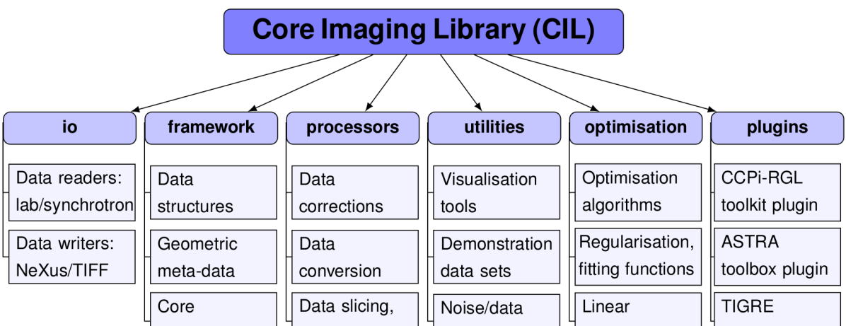
Figure 1: Overview of CIL module structure and contents. The cil.plugins module contains wrapper code for other software and third-party libraries that need to be installed separately to be used by CIL.

As a running example (Fig. 2) we employ a 3D parallel-beam X-ray CT data set from Beamline I13-2, Diamond Light Source, Harwell, UK. The sample consisted of a 0.5 mm aluminium cylinder with a piece of steel wire embedded in a small drilled hole. A droplet of salt water was placed on top, causing corrosion to form hydrogen bubbles. The data set, which was part of a fast time-lapse experiment, consists of 91 projections over 180^∘, originally acquired as size 2560-by-2160 pixels, but provided in [22] downsampled to 160-by-135 pixels.

2.1 Data readers and writers

Tomographic data comes in a variety of different formats depending on the instrument manufacturer or imaging facility. CIL currently supplies a native reader for Nikon’s XTek data format, Zeiss’ TXRM format, the NeXus format [23] if exported by CIL, as well as TIFF stacks. Here “native” means that a CIL AcquisitionData object incl. geometry (as described in the following subsection) will be created by the CIL reader. Other data formats can be read using e.g. DXchange [24] and a CIL AcquisitionData object can be manually constructed. CIL currently provides functionality to export/write data to disk in NeXus format or as a TIFF stack.

The steel-wire dataset is included as an example in CIL. It is in NeXus format and can be loaded using NEXUSDataReader. For example data sets in CIL we provide a convenience method that saves the user from typing the path to the datafile:

2.2 Data structures, geometry and core functionality

CIL provides two essential classes for data representation, namely AcquisitionData for tomographic data and ImageData for reconstructed (or simulated) volume data. The steel-wire dataset was read in as an AcquisitionData that we can inspect with:

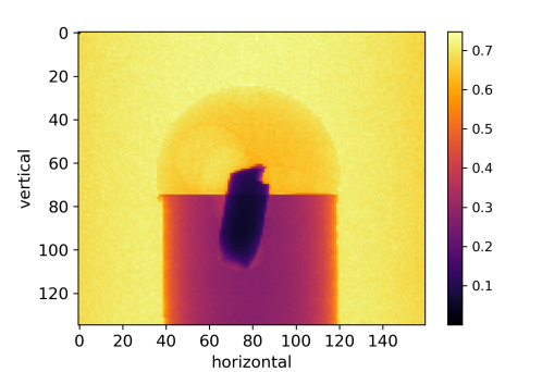
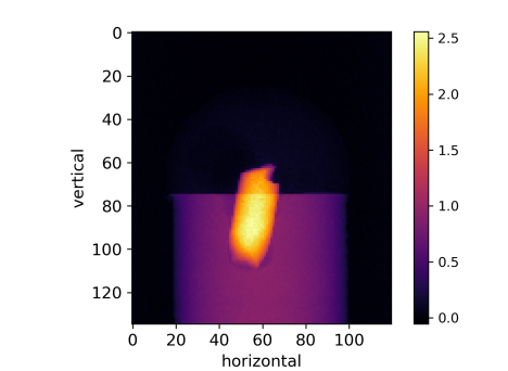
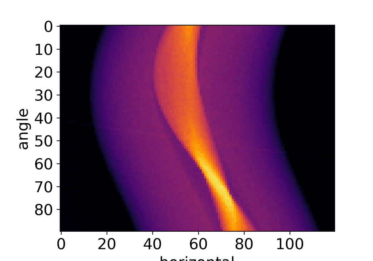
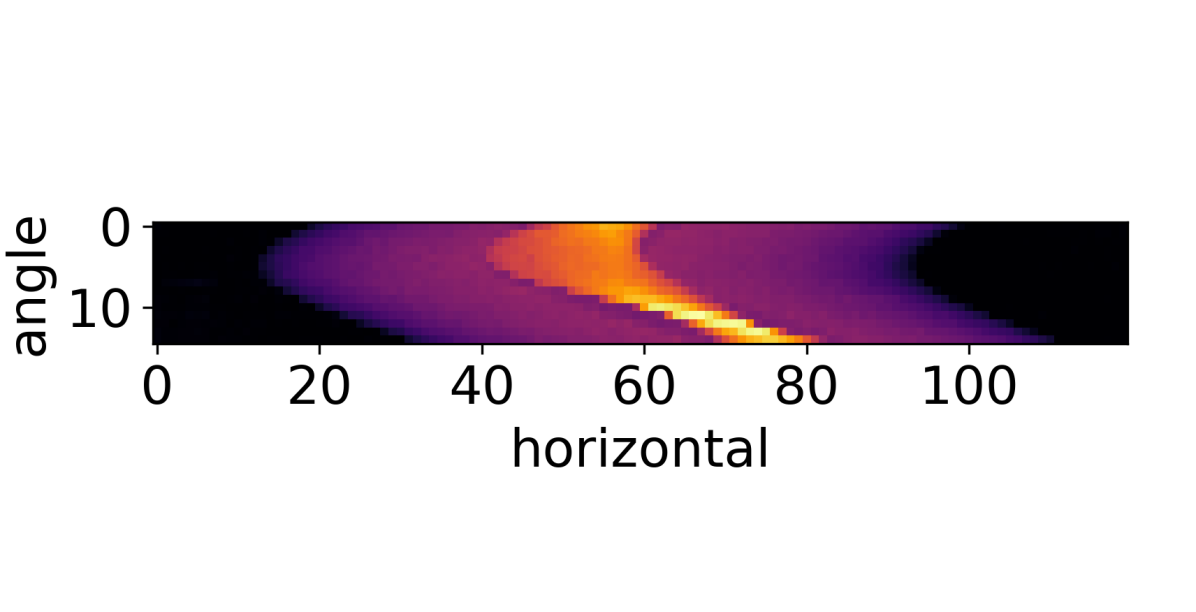
Figure 2: Raw and preprocessed 3D parallel-beam X-ray CT steel-wire dataset. Left: Raw transmission projection. Centre: Scaled, cropped, centred and negative-log transformed projection. Right, top: Sinogram for slice vertical=103, all 90 angles. Right, bottom: Same, subsampled to 15 equi-spaced angles.

At present, data is stored internally as a NumPy array and may be returned using the method as_array(). AcquisitionData and ImageData use string labels rather than a positional index to represent the dimensions. In the example data, ’angle’, ’vertical’ and ’horizontal’ refer to 91 projections each with vertical size 135 and horizontal size 160. Labels enable the user to access subsets of data without knowing the details of how it is stored underneath. For example we can extract a single projection using the method get_slice with the label and display it (Fig. 2 left) as

where show2D is a display functiontter in cil.utilities.display. show2D displays dimension labels on plot axes as in Fig. 2; subsequent plots omit these for space reasons.

Both ImageData and AcquisitionData behave much like a NumPy array with support for:

• algebraic operators +, -, etc.,

• relational operators ¿, ¿=, etc.,

• common mathematical functions like exp, log and abs, mean, and

• inner product dot and Euclidean norm norm.

This makes it easy to do a range of data processing tasks. For example in Fig. 2 (left) we note the projection (which is already flat-field normalised) has values around 0.7 in the background, and not 1.0 as in typical well-normalised data. This may lead to reconstruction artifacts. A quick-fix is to scale the image to have background value ca. 1.0. To do that we extract a row of the data toward the top, compute its mean and use it to normalise the data:

Where possible in-place operations are supported to avoid unnecessary copying of data. For example the Lambert-Beer negative logarithm conversion can be done by:

Geometric meta-data such as voxel dimensions and scan configuration is stored in ImageGeometry and AcquisitionGeometry objects available in the attribute geometry of ImageData and AcquisitionData. AcquisitionGeometry will normally be provided as part of an AcquisitionData produced by the CIL reader. It is also possible to manually create AcquisitionGeometry and ImageGeometry from a list of geometric parameters. Had the steel-wire dataset not had geometry information included, we could have set up its geometry with the following call:

The first line creates a default 3D parallel-beam geometry with a rotation axis perpendicular to the beam propagation direction. The second and third lines specify the detector dimension and the angles at which projections are acquired. Numerous configuration options are available for bespoke geometries; this is illustrated in Section 4.2, see in particular Fig. 9, for an example of cone-beam laminography. Similarly, ImageGeometry holds the geometric specification of a reconstructed volume, including numbers and sizes of voxels.

2.3 Preprocessing data

In CIL a Processor is a class that takes an ImageData or AcquisitionData as input, carries out some operations on it and returns an ImageData or AcquisitionData. Example uses include common preprocessing tasks such as resizing (e.g. cropping or binning/downsampling) data, flat-field normalization and correction for centre-of-rotation offset, see Table 1 for an overview of Processors currently in CIL.

Table 1: Processors currently available in CIL.

Name	Description
Binner	Downsample data in selected dimensions
CentreOfRotationCorrector	Find and correct for centre-of-rotation offset
Normaliser	Apply flat and dark field correction/normalisation
Padder	Pad/extend data in selected dimensions
Slicer	Extract data at specified indices
Masker	Apply binary mask to keep selected data only
MaskGenerator	Make binary mask to keep selected data only
RingRemover	Remove sinogram stripes to reduce ring artifacts

We will demonstrate centre-of-rotation correction and cropping using a Processor. Typically it is not possible to align the rotation axis perfectly with respect to the detector, and this leads to well-known centre-of-rotation reconstruction artifacts. CIL provides different techniques to estimate and compensate, the simplest being based on cross-correlation on the central slice. First the Processor instance must be created; this is an object instance which holds any parameters specified by the user; here which slice to operate on. Once created the Processor can carry out the processing task by calling it on the targeted data set. All this can be conveniently achieved in a single code line, as shown in the first line below.

Afterwards, we use a Slicer to remove some of the empty parts of the projections by cropping 20 pixel columns on each side of all projections, while also discarding the final projection which is a mirror image of the first. This produces data90. We can further produce a subsampled data set data15 by using another Slicer, keeping only every sixth projection.

Figure 2 illustrates preprocessing and the final 90- and 15-projection sinograms; mainly the latter will be used in what follows to highlight differences between reconstruction methods.

2.4 Auxiliary tools

This module contains a number of useful tools:

• dataexample: Example data sets and test images such as the steel-wire dataset.

• display: Tools for displaying data as images, including the show2D used in the previous section and other interactive displaying tools for Jupyter notebooks.

• noise: Tools to simulate different kinds of noise, including Gaussian and Poisson.

• quality_measures: Mathematical metrics Mean-Square-Error (MSE) and Peak-Signal-to-Noise-Ratio (PSNR) to quantify image quality against a ground-truth image.

Some of these tools are demonstrated in other sections of the present paper; for the rest we refer the reader to the CIL documentation.

2.5 CIL Plugins and interoperability with SIRF

CIL allows the use of third-party software through plugins that wrap the desired functionality. At present the following three plugins are provided:

• cil.plugins.ccpi_regularisation This plugin wraps a number of regularisation methods from the CCPi-RGL toolkit [16] as CIL Functions.

• cil.plugins.astra: This plugin provides access to CPU and GPU-accelerated forward and back projectors in ASTRA as well as the filtered back-projection (FBP) and Feldkamp-Davis-Kress (FDK) reconstruction methods for parallel and cone-beam geometries.

• cil.plugins.tigre: This plugin currently provides access to GPU-accelerated cone-beam forward and back projectors and the FDK reconstruction method of the TIGRE toolbox.

Furthermore, CIL is developed to be interoperable with the Synergistic Image Reconstruction Framework (SIRF) for PET and MR imaging [17]. This was achieved by synchronising naming conventions and basic class concepts:

• sirf: Data structures and acquisition models of SIRF can be used from CIL without a plugin, in particular with cil.optimisation one may specify and solve optimisation problems with SIRF data. An example of this using PET data is given in Section 4.3.

We demonstrate here how the cil.plugins.astra plugin, or cil.plugins.tigre plugin interchangeably, can be used to produce an FBP reconstruction of the steel-wire dataset using its FBP Processor. To compute a reconstruction we must specify the geometry we want for the reconstruction volume; for convenience, a default ImageGeometry can be determined from a given AcquisitionGeometry. The FBP Processor can then be set up and in this instance we specify for it to use GPU-acceleration, and then call it on the data set to produce a reconstruction:

The first line permutes the underlying data array to the specific dimension order required by cil.plugins.astra, which may differ from how data is read into CIL. Reconstructions for both the 90- and 15-projection steel-wire datasets are seen in Fig. 3, with notable streak artifacts in the subsampled case, as is typical with few projections.

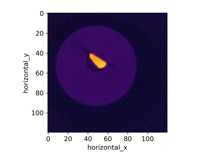
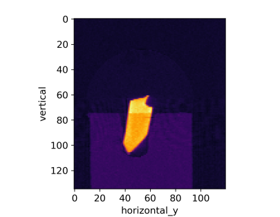
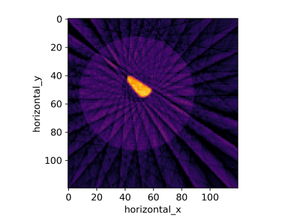
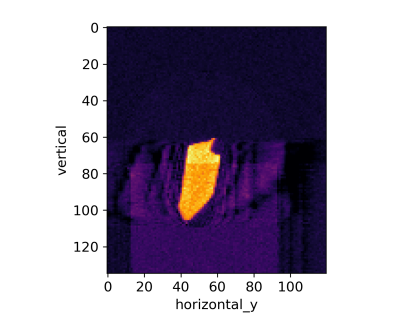
Figure 3: Reconstructions of steel-wire dataset by FBP. Left two: Horizontal and vertical slice using 90 projections. Right two: Same using 15 projections – showing prominent streak artifacts. Colour range [-0.01, 0.11].

3 Reconstruction by solving optimisation problems

FBP type reconstruction methods have very limited capability to model and address challenging data sets. For example the type and amount of noise cannot be modelled and prior knowledge such as non-negativity or smoothness cannot be incorporated. A much more flexible class of reconstruction methods arises from expressing the reconstructed image as the solution to an optimisation problem combining data and noise models and any prior knowledge.

The CIL optimisation module makes it simple to specify a variety of optimisation problems for reconstruction and provides a range of optimisation algorithms for their solution.

3.1 Operators

The ccpi.optimisation module is built around the generic linear inverse problem

$$Au=b,$$ (1)

where $A$ is a linear operator, $u$ is the image to be determined, and $b$ is the measured data. In CIL $u$ and $b$ are normally represented by ImageData and AcquisitionData respectively, and $A$ by a LinearOperator. The spaces that a LinearOperator maps from and to are represented in attributes domain and range; these should each hold an ImageGeometry or AcquisitionGeometry that match with that of $u$ and $b$, respectively.

Reconstruction methods rely on two essential methods of a LinearOperator, namely direct, which evaluates $Av$ for a given $v$, and adjoint, which evaluates $A^{*}z$ for a given $z$, where $A^{*}$ is the adjoint operator of $A$. For example, in a LinearOperator representing the discretised Radon transform for tomographic imaging, direct is forward projection, i.e., computing the sinogram corresponding to a given image, while adjoint corresponds to back-projection.

Table 2 provides an overview of the Operators available in the current version of CIL. It includes imaging models such as BlurringOperator for image deblurring problems and mathematical operators such as IdentityOperator and GradientOperator to act as building blocks for specifying optimisation problems. Operators can be combined to create new Operators through addition, scalar multiplication and composition.

The bottom two row contains ProjectionOperator from both cil.plugins.astra and cil.plugins.tigre, which wraps forward and back-projectors from the ASTRA and TIGRE toolboxes respectively, and can be used interchangeably. A ProjectionOperator can be set up simply by

and from the AcquisitionGeometry provided the relevant 2D or 3D, parallel-beam or cone-beam geometry employed; in case of the steel-wire dataset, a 3D parallel-beam geometry.

Table 2: Operators in CIL; and Operators from cil.plugins.astra and cil.plugins.tigre in bottom two rows.

Name	Description
BlockOperator	Form block (array) operator from multiple operators
BlurringOperator	Apply point spread function to blur an image
ChannelwiseOperator	Apply the same Operator to all channels
DiagonalOperator	Form a diagonal operator from image/acquisition data
FiniteDifferenceOperator	Apply finite differences in selected dimension
GradientOperator	Apply finite difference to multiple/all dimensions
IdentityOperator	Apply identity operator, i.e., return input
MaskOperator	From binary input, keep selected entries, mask out rest
SymmetrisedGradientOperator	Apply symmetrised gradient, used in TGV
ZeroOperator	Operator of all zeroes
ProjectionOperator	Tomography forward/back-projection from ASTRA
ProjectionOperator	Tomography forward/back-projection from TIGRE

3.2 Algebraic iterative reconstruction methods

One of the most basic optimisation problems for reconstruction is least-squares minimisation,

$$u^{\star}=\operatorname*{arg\,min}_{u}\|Au-b\|_{2}^{2},$$ (2)

where we seek to find the image $u$ that fits the data the best, i.e., in which the norm of the residual $Au-b$ takes on the smallest possible value; this $u$ we denote $u^{\star}$ and take as our reconstruction.

The Conjugate Gradient Least Squares (CGLS) algorithm [25] is an algebraic iterative method that solves exactly this problem. In CIL it is available as CGLS, which is an example of an Algorithm object. The following code sets up a CGLS algorithm – inputs required are an initial image, the operator (here ProjectionOperator from cil.plugins.astra), the data and an upper limit on the number iterations to run – and runs a specified number of iterations with verbose printing:

At this point the reconstruction is available as myCGLS.solution and can be displayed or otherwise analysed. The object-oriented design of Algorithm means that iterating can be resumed from the current state, simply by another myCGLS.run call.

As imaging operators are often ill-conditioned with respect to inversion, small errors and inconsistencies tend to magnify during the solution process, typically rendering the final least squares $u^{\star}$ useless. CGLS exhibits semi-convergence [26] meaning that in the initial iterations the solution will approach the true underlying solution, but from a certain point the noise will increasingly contaminate the solution. The number of iterations therefore has an important regularising effect and must be chosen with care.

CIL also provides the Simultaneous Iterative Reconstruction Technique (SIRT) as SIRT, which solves a particular weighted least-squares problem [27, 9]. As with CGLS, it exhibits semi-convergence, however tends to require more iterations. An advantage of SIRT is that it admits the specification of convex constraints, such as a box constraints (upper and lower bounds) on $u$; this is done using optional input arguments lower and upper:

In Fig. 4 we see that CGLS reduces streaks but blurs edges. SIRT further reduces streaks and sharpens edges to the background; this is an effect of the nonnegativity constraint. In the steel wire example data the upper bound of 0.09 is attained causing a more uniform appearance with sharper edges.

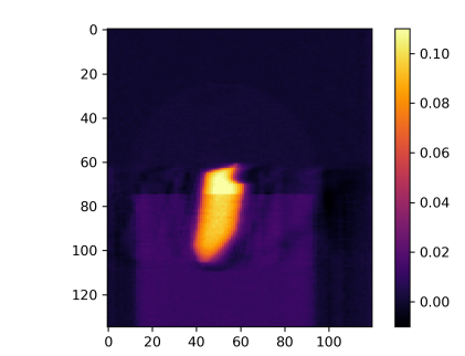
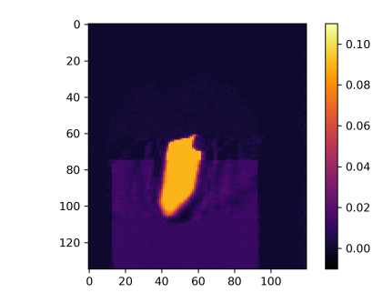
Figure 4: Algebraic iterative reconstruction of 15-projection 3D steel-wire dataset. Left two: Horizontal and vertical slices, 20-iteration CGLS reconstruction. Right two: Same using SIRT, lower/upper bounds 0.0/0.09. Colour range [-0.01,0.11].

3.3 Tikhonov regularisation with BlockOperator and BlockDataContainer

Algebraic iterative methods like CGLS and SIRT enforce regularisation of the solution implicitly by terminating iterations early. A more explicit form of regularisation is to include it directly in an optimisation formulation. The archetypal such method is Tikhonov regularisation which takes the form

$$u^{\star}=\operatorname*{arg\,min}_{u}\left\{\|Au-b\|_{2}^{2}+\alpha^{2}\|Du\|_{2}^{2}\right\},$$ (3)

where $D$ is some operator, the properties of which govern the appearance of the solution. In the simplest form $D$ can be taken as the identity operator. Another common choice is a discrete gradient implemented as a finite-difference operator. The regularisation parameter $\alpha$ governs the balance between the data fidelity term and the regularisation term. Conveniently, Tikhonov regularisation can be analytically rewritten as an equivalent least-squares problem, namely

$$u^{\star}=\operatorname*{arg\,min}_{u}\left\|\tilde{A}u-\tilde{b}\right\|_{2}^{2},\qquad\text{where}\qquad\tilde{A}=\binom{A}{\alpha D}\quad\text{and}\quad\tilde{b}=\binom{b}{0},$$ (4)

where the $0$ corresponds to the range of $D$. We can use the CGLS algorithm to solve Eq. 4 but we need a way to express the block structure of $\tilde{A}$ and $\tilde{b}$. This is achieved by the BlockOperator and BlockDataContainer of CIL:

If instead we want the discrete gradient as $D$ we simply replace the second line by:

GradientOperator automatically works out from the ImageGeometry ig which dimensions are available and sets up finite differencing in all dimensions. If two or more dimensions are present, D will in fact be a BlockOperator with a finite-differencing block for each dimension. CIL supports nesting of a BlockOperator inside another, so that Tikhonov regularisation with a Gradient operator can be conveniently expressed.

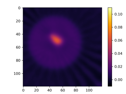
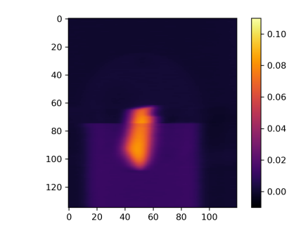
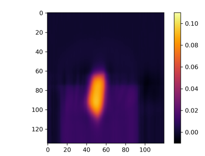
Figure 5: Anisotropic Tikhonov reconstruction of 15-projection 3D steel-wire dataset. Left two: Horizontal and vertical slices, Tikhonov regularisation with horizontal smoothing ($\alpha_{x}=\alpha_{y}=30$, $\alpha_{z}=0.1$). Right two: Same, with vertical smoothing ($\alpha_{x}=\alpha_{y}=0.1$, $\alpha_{z}=60$). Colour range [-0.01,0.11].

In Fig. 5 (left) Tikhonov regularisation with the GradientOperator is demonstrated on the steel-wire sample. Here, $\alpha$ governs the solution smoothness similar to how the number of iterations affects CGLS solutions, with large $\alpha$ values producing smooth solutions. Here $\alpha=1$ is used as a suitable trade-off between noise reduction and smoothing.

The block structure provides the machinery to experiment with different amounts or types of regularisation in individual dimensions in a Tikhonov setting. We consider the problem

$$u^{\star}=\operatorname*{arg\,min}_{u}\left\{\|Au-b\|_{2}^{2}+\alpha_{x}^{2}\|D_{x}u\|_{2}^{2}+\alpha_{y}^{2}\|D_{y}u\|_{2}^{2}+\alpha_{z}^{2}\|D_{z}u\|_{2}^{2}\right\},$$ (5)

where we have different regularising operators $D_{x}$, $D_{y}$, $D_{z}$ in each dimension and associated regularisation parameters $\alpha_{x}$, $\alpha_{y}$, $\alpha_{z}$. We can write this as the following block least squares problem which can be solved by CGLS:

$$u^{\star}=\operatorname*{arg\,min}_{u}\left\|\begin{pmatrix}A\\ \alpha_{x}D_{x}\\ \alpha_{y}D_{y}\\ \alpha_{z}D_{z}\\ \end{pmatrix}u-\begin{pmatrix}b\\ 0_{x}\\ 0_{y}\\ 0_{z}\\ \end{pmatrix}\right\|_{2}^{2},$$ (6)

where $0_{x}$, $0_{y}$ and $0_{z}$ represent zero vectors of appropriate size.

In Fig. 5 we show results for $D_{x}$, $D_{y}$ and $D_{z}$ being finite-difference operators in each direction, achieved by the FiniteDifferenceOperator. We show two choices of sets of regularisation parameters, namely $\alpha_{x}=\alpha_{y}=30$, $\alpha_{z}=0.1$ and $\alpha_{x}=\alpha_{y}=0.1$, $\alpha_{z}=60$. We see in the former case a large amount of smoothing occurs in the horizontal dimensions due to the larger $\alpha_{x}$ and $\alpha_{y}$ parameters, and little in the vertical dimension, so horizontal edges are preserved. In the latter case, opposite observations can be made.

Such anisotropic regularization could be useful with objects having a layered or fibrous structure or if the measurement setup provides different resolution or noise properties in different dimensions, e.g., for non-standard scan trajectories such as tomosynthesis/laminography.

3.4 Smooth convex optimisation

Table 3: Functions in CIL.

Name	Description
BlockFunction	Separable sum of multiple functions
ConstantFunction	Function taking the constant value
OperatorCompositionFunction	Compose function $f$ and operator $A$: $f(Ax)$
IndicatorBox	Indicator function for box (lower/upper) constraints
KullbackLeibler	Kullback-Leibler divergence data fidelity
L1Norm	$L^{1}$-norm: $\|x\|_{1}=\sum_{i}|x_{i}|$
L2NormSquared	Squared $L^{2}$-norm: $\|x\|_{2}^{2}=\sum_{i}x_{i}^{2}$
LeastSquares	Least-squares data fidelity: $\|Ax-b\|_{2}^{2}$
MixedL21Norm	Mixed $L^{2,1}$-norm: $\|(U_{1};U_{2})\|_{2,1}=\|(U_{1}^{2}+U_{2}^{2})^{1/2}\|_{1}$
SmoothMixedL21Norm	Smooth $L^{2,1}$-norm: $\|(U_{1};U_{2})\|_{2,1}^{\text{S}}=\|(U_{1}^{2}+U_{2}^{2}+\beta^{2})^{1/2}\|_{1}$
WeightedL2NormSquared	Weighted squared $L^{2}$-norm: $\|x\|_{w}^{2}=\sum_{i}(w_{i}\cdot x_{i}^{2})$

CIL supports the formulation and solution of more general optimisation problems. One problem class supported is unconstrained smooth convex optimisation problems,

$$u^{\star}=\operatorname*{arg\,min}_{u}f(u).$$ (7)

Here $f$ is a differentiable, convex, so-called $L$-smooth function, that is its gradient $\nabla f$ is $L$-Lipschitz continuous: $\|\nabla f(u_{1})-\nabla f(u_{2})\|_{2}\leq L\|u_{1}-u_{2}\|_{2},\;\forall u_{1},u_{2}$ for some $L>0$ referred to as the Lipschitz parameter. CIL represents functions by the Function class, which maps an ImageData or AcquisitionData to a real number. Differentiable functions provide the method gradient to allow first-order optimisation methods to work; at present CIL provides a Gradient Descent method GD with a constant or back-tracking line search for step size selection. CIL Function supports algebra so the user can formulate for example linear combinations of Function objects and solve with the GD algorithm.

As example we can formulate and solve the Tikhonov problem Eq. 3 with GD as

Here LeastSquares(A,b), representing $\|A\cdot-b\|_{2}^{2}$, and L2NormSquared, representing $\|\cdot\|_{2}^{2}$, are examples from the Function class. With OperatorCompositionFunction a function can be composed with an operator, here L, to form a composite function $\|L\cdot\|_{2}^{2}$. An overview of Function types currently in CIL is provided in Table 3. Another example using a smooth approximation of non-smooth total variation regularisation will be given in Section 4.1.

3.5 Non-smooth convex optimisation with simple proximal mapping

Figure 6: FISTA reconstruction of 15-projection 3D steel-wire dataset. Left two: $L^{1}$-norm regularization with large regularisation parameter of $\alpha=30$ forces all pixels but in steel wire to zero. Right two: TV-regularisation with $\alpha=0.02$ removes streaks and noise and preserves edges. Colour range [-0.01,0.11].

Many useful reconstruction methods are formulated as non-smooth optimisation problems. Of specific interest in recent years has been sparsity-exploiting regularisation such as the $L^{1}$-norm and total variation (TV). TV-regularisation for example has been shown capable of producing high-quality images from severely undersampled data whereas FBP produces highly noisy, streaky images. A particular problem class of interest can be formulated as

$$u^{\star}=\operatorname*{arg\,min}_{u}\Big{\{}f(u)+g(u)\Big{\}},$$ (8)

where $f$ is $L$-smooth and $g$ may be non-smooth. This problem can be solved by the Fast Iterative Shrinkage-Thresholding Algorithm (FISTA) [28, 29], which is available in CIL as FISTA. FISTA makes use of $f$ being smooth by calling f.gradient and assumes for $g$ that the so-called proximal mapping,

$$\mathrm{prox}_{\tau g}(u)=\operatorname*{arg\,min}_{v}\left\{\tau g(v)+\frac{1}{2}\|v-u\|_{2}^{2}\right\}$$ (9)

for a positive parameter $\tau$ is available as g.proximal. This means that FISTA is useful when $g$ is “proximable”, i.e., where an analytical expression for the proximal mapping exists, or it can be computed efficiently numerically.

A simple, but useful case, for FISTA is to enforce constraints on the solution, i.e., require $u\in C$, where $C$ is a convex set. In this case $g$ is set to the (convex analysis) indicator function of $C$, i.e.,

$$\iota_{C}(u)=\left\{\begin{array}[]{lll}0&\text{if}&u\in C\\ \infty&\text{else}.&\end{array}\right.$$ (10)

The proximal mapping of an indicator function is simply a projection onto the convex set; for simple lower and upper bound constraints this is provided in CIL as IndicatorBox. FISTA with non-negativity constraints is achieved with the following lines of code:

Another simple non-smooth case is $L^{1}$-norm regularisation, i.e., using $\|u\|_{1}=\sum_{j}|u_{j}|$ as regulariser. This is non-differentiable at $0$ and a closed-form expression for the proximal mapping is known as the so-called soft-thresholding. In CIL this is available as L1Norm and can be achieved with the same code, only with the second line replaced by

The resulting steel-wire dataset reconstruction is shown in Fig. 6.

FISTA can also be used whenever a numerical method is available for the proximal mapping of $g$; one such case is the (discrete, isotropic) Total Variation (TV). TV is the mixed $L^{2,1}$-norm of the gradient image,

$$g_{\text{TV}}(u)=\|Du\|_{2,1}=\left\|\binom{D_{x}}{D_{y}}u\right\|_{2,1}=\left\|\sqrt{(D_{x}u)^{2}+(D_{y}u)^{2}}\right\|_{1},$$ (11)

where $D=(D_{x};D_{y})$ is the gradient operator as before and the $L^{2}$-norm combines the $x$ and $y$ differences before the $L^{1}$-norm sums over all voxels. CIL implements this in TotalVariation using the FGP method from [29]. Using the FISTA code above we can achieve this with

The resulting reconstruction is shown in Fig. 6 and clearly demonstrates the edge-preserving, noise-reducing and streak-removing capabilities of TV-regularisation.

3.6 Non-smooth convex optimisation using splitting methods

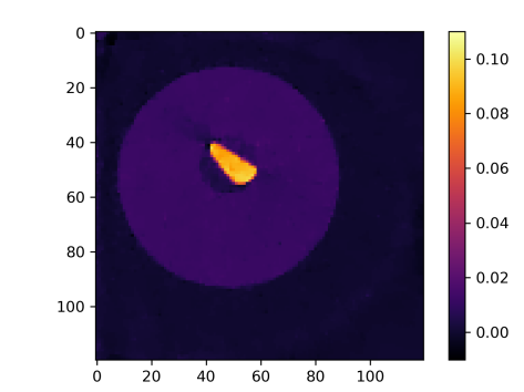
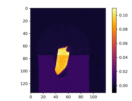
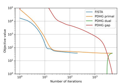
Figure 7: PDHG reconstruction of 15-projection 3D steel-wire dataset. Left two: TV-regularisation with $\alpha=0.02$, reproduces same result as FISTA in Fig. 6 on same case and parameter choice, thus validating algorithms against each other. Colour range [-0.01,0.11]. Right: Objective value histories (log-log) for FISTA and PDHG on TV-regularisation problem. Both algorithms reach the same (primal) objective value, FISTA taking fewer but slower iterations. The primal-dual gap for PDHG (difference between primal and dual objectives) approaches zero indicating convergence.

When the non-smooth function is not proximable, we may consider so-called splitting methods for solving a more general class of problems, namely

$$u^{\star}=\operatorname*{arg\,min}_{u}\Big{\{}f(Ku)+g(u)\Big{\}},$$ (12)

where $f$ and $g$ are convex (possibly) non-smooth functions and $K$ a linear operator. The key change from the FISTA problem is the splitting of the complicated $f(K(u))$, which as a whole may not be proximable, into simpler parts $f$ and $K$ to be handled separately. CIL provides two algorithms for solving this problem, depending on properties of $f$ and assuming that $g$ is proximable. If $f$ is proximable, then the linearised ADMM method [30] can be used; available as LADMM in CIL. If the so-called convex conjugate, $f^{*}$, of $f$ is proximable, then the Primal Dual Hybrid Gradient (PDHG) method [31, 32, 33], also known as the Chambolle-Pock method, may be used; this is known as PDHG in CIL.

Table 4: Algorithms in CIL.

Name	Description	Problem type solved
CGLS	Conjugate Gradient Least Squares	Least squares
SIRT	Simultaneous Iterative Reconstruction Technique	Weighted least squares
GD	Gradient Descent	Smooth
FISTA	Fast Iterative Shrinkage-Thresholding Algorithm	Smooth + non-smooth
LADMM	Linearised Alternating Direction Method of Multipliers	Non-smooth
PDHG	Primal Dual Hybrid Gradient	Non-smooth
SPDHG	Stochastic Primal Dual Hybrid Gradient	Non-smooth

In fact an even wider class of problems can be handled using this formulation, namely

$$u^{\star}=\operatorname*{arg\,min}_{u}\left\{\sum_{i}f_{i}(K_{i}u)+g(u)\right\},$$ (13)

i.e., where the composite function $f(K\cdot)$ can be written as a separable sum

$$f(Ku)=\sum_{i}f_{i}(K_{i}u).$$ (14)

In CIL we can express such a function using a BlockOperator, as also used in the Tikhonov example, and a BlockFunction, which essentially holds a list of Function objects.

Here we demonstrate this setup by using PDHG to solve the TV-regularised least-squares problem. As shown in [33] this problem can be written in the required form as

$$f=\binom{f_{1}}{f_{2}}=\binom{\|\cdot-b\|_{2}^{2}}{\alpha\|\cdot\|_{2,1}},\qquad K=\binom{A}{D},\qquad g(u)=0.$$ (15)

In CIL this can be written succinctly as (with a specific choice of regularisation parameter):

Figure 7 shows the resulting steel-wire dataset reconstruction which appears identical to the result of FISTA on the same problem (Fig. 6), and as such validates the two algorithms against each other.

CIL Algorithms have the option to save the history of objective values so the progress and convergence can be monitored. PDHG is a primal-dual algorithm, which means that the so-called dual maximisation problem of Eq. 12, which is referred to as the primal problem, is solved simultaneously. In PDHG the dual objective values are also available. The primal-dual gap, which is the difference between the primal and dual objective values, is useful for monitoring convergence as it should approach zero when the iterates converge to the solution.

Figure 7 (right) compares the primal objective, dual objective and primal-dual gap history with the objective history for FISTA on the same problem. The (primal) objectives settle at roughly the same level, again confirming that the two algorithms achieve essentially the same solution. FISTA used fewer iterations, but each iteration took about 25 times as long as a PDHG iteration. The dual objective is negative until around 3000 iterations, and the primal-dual gap is seen to approach zero, thus confirming convergence. CIL makes such algorithm comparisons straightforward. It should be stressed that the particular convergence behavior observed for FISTA and PDHG depends on internal algorithm parameters such as step sizes for which default values were used here. The user may experiment with tuning these parameters to obtain faster convergence, for example for PDHG the primal and dual step sizes may be set using the inputs sigma and tau.

In addition to PDHG a stochastic variant SPDHG [34] that can sometimes accelerate reconstruction substantially by working on problem subsets is provided in CIL as SPDHG; this is demonstrated in the Part II article [18].

An overview of all the algorithms currently supplied by CIL is provided in Table 4.

4 Exemplar studies using CIL

This section presents 3 illustrative examples each demonstrating different functionality of CIL. All code and data to reproduce the results are provided, see Data Accessibility.

4.1 Neutron tomography with golden-angle data

This example demonstrates how CIL can handle other imaging modalities than X-ray, a non-standard scan geometry, and easily compare reconstruction algorithms.

Contrary to X-rays, neutrons interact with atomic nuclei rather than electrons that surround them, which yields a different contrast mechanism, e.g., for neutrons hydrogen is highly attenuating while lead is almost transparent. Nevertheless, neutron data can be modelled with the Radon transform and reconstructed with the same techniques as X-ray data.

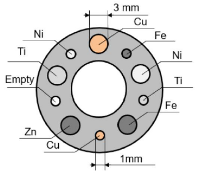
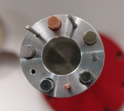
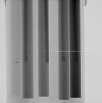
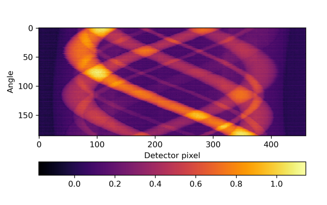
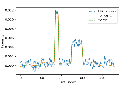
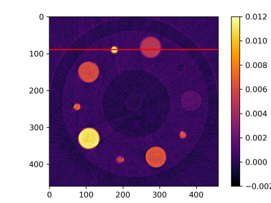
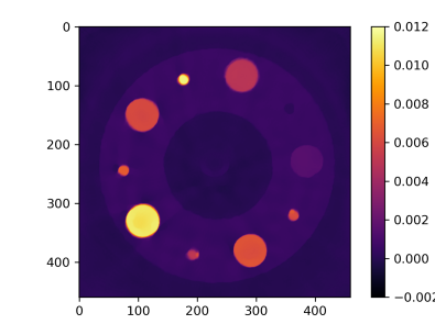
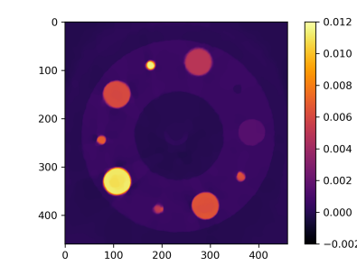
Figure 8: IMAT neutron tomography dataset. Top row: (left) top-view schematic of high-purity elemental metal rod sample; (centre) top-view photograph; (right) single raw projection image showing rods of different absorption. Middle row: (left) preprocessed slice sinogram; (right) horizontal line profile of FBP, PDHG TV and GD TV reconstruction along line shown on image below. Bottom row: (left) slice reconstructions, FBP; (centre) TV reconstruction with PDHG; (right) STV reconstruction with GD. Colour range [-0.002, 0.012].

A benchmarking neutron tomography dataset (Fig. 8) was acquired at the IMAT beamline [35, 36] of the ISIS Neutron and Muon Source, Harwell, UK. The raw data is available at [37] and a processed subset for this paper is available from [38]. The test phantom consisted of an Al cylinder of diameter 22 mm with cylindrical holes holding 1mm and 3mm rods of high-purity elemental Cu, Fe, Ni, Ti, and Zn rods. 186 projections each 512-by-512 pixels in size 0.055 mm were acquired using the non-standard golden-angle mode [39] (angular steps of $\frac{1}{2}(\sqrt{5}-1)\cdot 180^{\circ}=111.24...^{\circ}$) rather than sequential small angular increments. This was to provide complete angular coverage in case of early experiment termination and to allow experimenting with reconstruction from a reduced number of projections. An energy-sensitive micro-channel plate (MCP) detector was used [40, 41] providing raw data in 2332 energy bins per pixel, which were processed and summed to simulate a conventional white-beam absorption-contrast data set for the present paper. Reconstruction and analysis of a similar energy-resolved data set is given in [21].

We use TIFFStackReader to load the data, several Processor instances to preprocess it, and initially FBP to reconstruct it. We compare with TV-regularisation, Eq. 11, solved with MixedL21Norm and PDHG using $\alpha=1$ and 30000 iterations, and further with a smoothed variant of TV (STV) using SmoothMixedL21Norm. The latter makes the optimisation problem smooth, so it can be solved using GD, using the same $\alpha$ and 10000 iterations.

The sinogram for a single slice is shown in Fig. 8 along with FBP, TV and STV reconstructions and a horizontal line profile plot as marked by the red line. The FBP reconstruction recovers the main sample features, however it is contaminated by noise, ring artifacts and streak artifacts emanating from the highest-attenuating rods. The TV and STV reconstructions remove these artifacts, while preserving edges. We see that the STV approximates the non-smooth TV very well; this also serves to validate the reconstruction algorithms against one another.

4.2 Non-standard acquisition: X-ray laminography

This example demonstrates how even more general acquisition geometries can be processed using CIL, and how cil.plugins.ccpi_regularisation allows CIL to use GPU-accelerated implementations of regularising functions available in the CCPi-RGL toolkit [16]. Furthermore, unlike the examples up to now, we here employ the ProjectionOperator provided by the TIGRE plugin, though the ASTRA plugin could equally have been used.

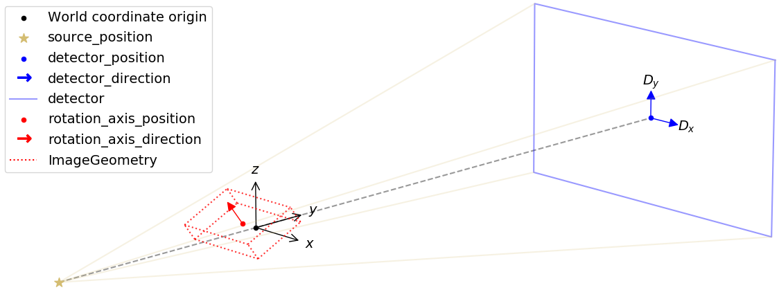
Figure 9: CIL AcquisitionGeometry and ImageGeometry illustrated for the laminography cone-beam setup. Configurable parameters are shown in the legend. Parallel-beam geometry and 2D versions are also available. CIL can illustrate ImageGeometry and AcquisitionGeometry instances as in this figure using show_geometry.

Laminography is an imaging technique designed for planar samples in which the rotation axis is tilted relative to the beam direction. Conventional imaging of planar samples often leads to severe limited-angle artifacts due to lack of transmission in-plane, while laminography can provide a more uniform exposure [42]. In Transmission Electron Microscopy (TEM) the same technique is known as conical tilt.

An experimental laminography setup in the so-called rotary configuration was developed [43] for Nikon micro-CT scanners in the Manchester X-ray Imaging Facility. Promising reconstructions of a planar LEGO-brick test phantom were obtained using the CGLS algorithm. Here we use CIL on the same data [44] to demonstrate how TV-regularisation and non-negativity constraints can reduce inherent laminographic reconstruction artifacts. CIL allows the specification of very flexible scan configurations. The cone-beam laminography setup of the LEGO data set provides an illustrative case for demonstrating CIL geometry, see Fig. 9. This particular geometry can be specified as follows, illustrating how different geometry components are used:

The data consists of 2512 projections of 798-by-574 pixels sized 0.508 mm in a 360^∘ cone-beam geometry. We load the data with NikonDataReader and preprocess with a couple of Processor instances to prepare it for reconstruction. For reconstruction we use the GPU-accelerated cone-beam ProjectionOperator from ccpi.plugin.tigre and FISTA to solve Eq. 8 for the unregularised least-squares problem (LS) and non-negativity constrained TV-regularised least-squares (TVNN). For TVNN we use FBP_TV from cil.plugins.ccpi_regularisation which implements a GPU-accelerated version of $g_{\text{TV}}$, which is faster than, but otherwise equivalent to, using the native CIL TotalVariation. The full 3D volume is reconstructed for LS and TVNN, and Fig. 10 shows a horizontal and vertical slice through both.

The LEGO bricks are clearly visualised in all reconstructions. The LS reconstruction has a haze in the horizontal slice (top left), which in the vertical slice (bottom left) is seen to amount to smooth directional streaks known to be inherent for laminography; in particular horizontal edges are heavily blurred. On the other hand, fine details in the horizontal plane are preserved, for example the text “LEGO” seen on several knobs to the right.

TVNN (right) reduces the haze and streaks substantially with the LEGO bricks displaying a uniform gray level and the horizontal edges in the vertical slice completely well-defined. However, some fine details are lost, including the “LEGO” text, which is a commonly observed drawback of TV-regularisation. Depending on the sample and application, this may or may not be an issue, and if necessary more sophisticated regularisers such as Total Generalised Variation (TGV) could be explored (a CIL example with TGV is given in the Part II article [18]).

As shown, CIL can process very general scan configurations and allows easy experimentation with different reconstruction methods, including using third-party software through plugins.

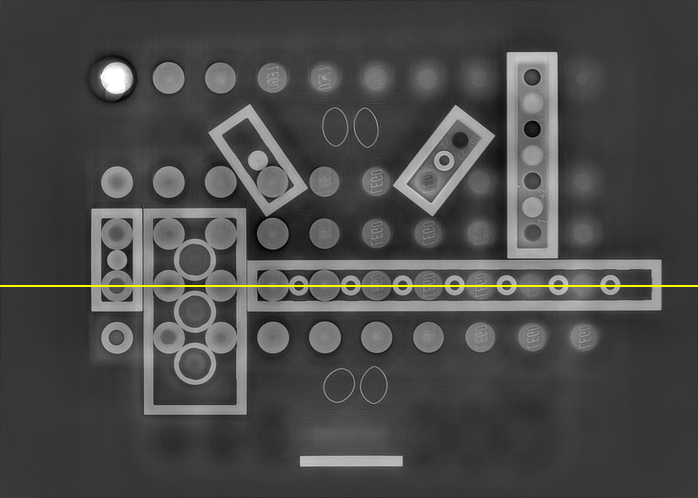
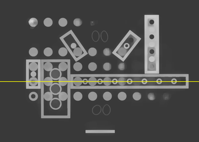
Figure 10: Slices through 3D reconstruction of laminography LEGO sample. Left, top/bottom: LS reconstruction using FISTA, horizontal/vertical slice at yellow line. Right: Same using TVNN, in which laminography artifact are suppressed while edges preserved.

4.3 PET reconstruction in CIL using SIRF

SIRF (Synergistic Image Reconstruction Framework) [17] is an open-source platform for joint reconstruction of PET and MRI data developed by CCP-SyneRBI (formerly CCP-PETMR). CIL and SIRF have been developed with a large degree of interoperability, in particular data structures are aligned to enable CIL algorithms to work directly on SIRF data. As an example we demonstrate here reconstruction of the NEMA IQ Phantom [45], which is a standard phantom for testing scanner and reconstruction performance. It consists of a Perspex container with inserts of different-sized spheres, some filled with liquid with higher radioactivity concentration than the background, others with “cold” water (see [45] for more details). This allows assessment of resolution and quantification.

A 60-minute PET dataset [46] of the NEMA IQ phantom was acquired on a Siemens Biograph mMR PET/MR scanner at Institute of Nuclear Medicine, UCLH, London. Due to poor data statistics in PET a Poisson noise model is normally adopted, which leads to using the Kullback-Leibler (KL) divergence as data fidelity. We compare here reconstruction using the Ordered Subset Expectation Maximisation (OSEM) method [47] available in SIRF without using CIL, and TV-regularised KL divergence minimisation using CIL’s PDHG algorithm with a KullbackLeibler data fidelity (KLTV). Instead of a CIL Operator a SIRF AcquisitionModel represents the forward model, and has all necessary methods to allow its use in CIL algorithms.

Figure 11 shows horizontal slices through the $220\times 220\times 127$-voxel OSEM and KLTV reconstructions and vertical profile plots along the red line. In both cases the inserts are visible, but OSEM is highly affected by noise. KLTV reduces the noise dramatically, while preserving the insert and outer phantom edges. This may be beneficial in subsequent analysis, however a more detailed comparative study should take post-filtering into account.

The purpose of this example was to give proof of principle of prototyping new reconstruction methods for PET with SIRF, using the generic algorithms of CIL, without needing to implement dedicated new algorithms in SIRF. Another example with SIRF for PET/MR motion compensation employing CIL is given in [19].

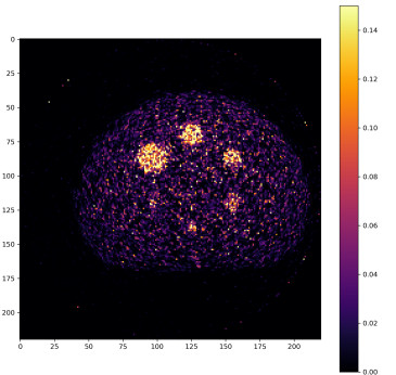
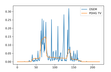
Figure 11: 3D PET reconstruction of NEMA IQ phantom data using CIL with SIRF data structures. Left: OSEM reconstruction (SIRF), horizontal slice. Centre: KLTV reconstruction (CIL PDHG). Colour range both [0,0.15]. Right: OSEM and KLTV profiles along red vertical line on centre plot.

5 Summary and outlook

We have described the CCPi Core Imaging Library (CIL), an open-source library, primarily written in Python, for processing tomographic data, with particular emphasis on enabling a variety of regularised reconstruction methods. The structure is highly modular to allow the user to easily prototype and solve new problem formulations that improve reconstructions in cases with incomplete or low-quality data. We have demonstrated the capability and flexibility of CIL across a number of test cases, including parallel-beam, cone-beam, non-standard (laminography) scan geometry, neutron tomography and PET using SIRF data structures in CIL. Further multi-channel cases including temporal/dynamic and spectral tomography are given in [18].

CIL remains under active development with continual new functionality being added, steered by ongoing and future scientific projects. Current plans include:

• adding more algorithms, functions, and operators to support an even greater set of problems, for example allow convex constraints in smooth problems;

• adding more pre-/postprocessing tools, for example to handle beam hardening;

• adding templates with preselected functions, algorithms, etc. to simplify solving common problems such as TV regularisation;

• further integrating with other third-party open-source tomography software through the plugin capability;

• introducing support for nonlinear problems, such as polarimetric neutron spin tomography [48] and electron strain tomography [49]; and

• developing support for multi-modality problems.

CIL is developed as open-source on GitHub, and questions, feature request and bug reports submitted as issues are welcomed. Alternatively, the developer team can be reached directly at CCPI-DEVEL@jiscmail.ac.uk. CIL is currently distributed through the Anaconda platform; in the future additional modes of distribution such as Docker images may be provided. Installation instructions, documentation and training material is available from https://www.ccpi.ac.uk/cil as well as at [4], as are GitHub repositories with source code that may be cloned/forked and built manually. In this way users may modify and contribute back to CIL.

Finally we emphasize that a multitude of optimization and regularization methods exist beyond those currently implemented in CIL and demonstrated in the present article. Recent overviews are given for example by [50, 51, 52, 3] with new problems and methods constantly being devised. CIL offers a modular platform to easily implement and explore such methods numerically as well as apply them directly in large-scale imaging applications.

Data accessibility

CIL version 21.0 as presented here is available through Anaconda; installation instructions are at https://www.ccpi.ac.uk/cil. In addition, CIL v21.0 and subsequent releases are archived at [4]. Python scripts to reproduce all results are available from [53]. The steel-wire data set is provided as part of CIL; the original data is at [22]. The neutron data set is available from [38]. The laminography data set is available from [44]. The NEMA IQ PET data set is available from [46].

Author contributions

JJ designed and coordinated the study, carried out the steel-wire and neutron case studies, wrote the manuscript, and conceived of and developed the CIL software. EA processed and analysed data for the neutron case study and developed the CIL software. GB co-designed, acquired, processed and analysed the neutron data. GF carried out the laminography case study and developed the CIL software. EPap carried out the PET case study and developed the CIL software. EPas conceived of and developed the CIL software and interoperability with SIRF. KT contributed to the PET case study, interoperability with SIRF and development of the CIL software. RW assisted with case studies and contributed to the CIL software. MT, WL and PW helped conceptualise and roll out the CIL software. All authors critically revised the manuscript, gave final approval for publication and agree to be held accountable for the work performed therein.

Competing interests

The authors declare that they have no competing interests.

Funding

The work presented here was funded by the EPSRC grants “A Reconstruction Toolkit for Multichannel CT” (EP/P02226X/1), “CCPi: Collaborative Computational Project in Tomographic Imaging” (EP/M022498/1 and EP/T026677/1), “CCP PET-MR: Computational Collaborative Project in Synergistic PET-MR Reconstruction” (EP/M022587/1) and “CCP SyneRBI: Computational Collaborative Project in Synergistic Reconstruction for Biomedical Imaging” (EP/T026693/1). We acknowledge the EPSRC for funding the Henry Moseley X-ray Imaging Facility through grants (EP/F007906/1, EP/F001452/1, EP/I02249X/1, EP/M010619/1, and EP/F028431/1) which is part of the Henry Royce Institute for Advanced Materials funded by EP/R00661X/1. JSJ was partially supported by The Villum Foundation (grant no. 25893). EA was partially funded by the Federal Ministry of Education and Research (BMBF) and the Baden-Württemberg Ministry of Science as part of the Excellence Strategy of the German Federal and State Governments. WRBL acknowledges support from a Royal Society Wolfson Research Merit Award. PJW and RW acknowledge support from the European Research Council grant No. 695638 CORREL-CT. We thank Diamond Light Source for access to beamline I13-2 (MT9396) that contributed to the results presented here, and Alison Davenport and her team for the sample preparation and experimental method employed. We gratefully acknowledge beamtime RB1820541 at the IMAT Beamline of the ISIS Neutron and Muon Source, Harwell, UK.

Acknowledgements

We are grateful to input from Daniil Kazantsev for early-stage contributions to this work. We are grateful to Josef Lewis for building the neutron experiment aluminium sample holder and help with sample preparation at IMAT. We wish to express our gratitude to numerous people in the tomography community for valuable input that helped shape this work, including Mark Basham, Julia Behnsen, Ander Biguri, Richard Brown, Sophia Coban, Melisande Croft, Claire Delplancke, Matthias Ehrhardt, Llion Evans, Anna Fedrigo, Sarah Fisher, Parmesh Gajjar, Joe Kelleher, Winfried Kochelmann, Thomas Kulhanek, Alexander Liptak, Tristan Lowe, Srikanth Nagella, Evgueni Ovtchinnikov, Søren Schmidt, Daniel Sykes, Anton Tremsin, Nicola Wadeson, Ying Wang, Jason Warnett, and Erica Yang. This work made use of computational support by CoSeC, the Computational Science Centre for Research Communities, through CCPi and CCP-SyneRBI.

References

- [1] Shearing P, Turner M, Sinclair I, Lee P, Ahmed F, Quinn P, et al.. EPSRC X-Ray Tomography Roadmap 2018; 2018. Available from: https://epsrc.ukri.org/files/research/epsrc-x-ray-tomography-roadmap-2018/.
- [2] Pan X, Sidky EY, Vannier M. Why do commercial CT scanners still employ traditional, filtered back-projection for image reconstruction? Inverse Problems. 2009;25(12):123009.
- [3] Zhang H, Wang J, Zeng D, Tao X, Ma J. Regularization strategies in statistical image reconstruction of low-dose x-ray CT: A review. Medical Physics. 2018;45(10):e886–e907.
- [4] Ametova E, Fardell G, Jørgensen JS, Papoutsellis E, Pasca E. Releases of Core Imaging Library (CIL). Zenodo; 2021. Available from: https://doi.org/10.5281/zenodo.4746198.
- [5] Gürsoy D, De Carlo F, Xiao X, Jacobsen C. TomoPy: a framework for the analysis of synchrotron tomographic data. Journal of Synchrotron Radiation. 2014;21(5):1188–1193.
- [6] van Aarle W, Palenstijn WJ, Cant J, Janssens E, Bleichrodt F, Dabravolski A, et al. Fast and flexible X-ray tomography using the ASTRA toolbox. Opt Express. 2016;24(22):25129–25147.
- [7] Biguri A, Dosanjh M, Hancock S, Soleimani M. TIGRE: a MATLAB-GPU toolbox for CBCT image reconstruction. Biomedical Physics & Engineering Express. 2016;2(5):055010.
- [8] Atwood RC, Bodey AJ, Price SWT, Basham M, Drakopoulos M. A high-throughput system for high-quality tomographic reconstruction of large datasets at Diamond Light Source. Philosophical Transactions of the Royal Society A. 2015;373:20140398.
- [9] Hansen PC, Jørgensen JS. AIR Tools II: algebraic iterative reconstruction methods, improved implementation. Numerical Algorithms. 2018;79:107–137.
- [10] Merlin T, Stute S, Benoit D, Bert J, Carlier T, Comtat C, et al. CASToR: a generic data organization and processing code framework for multi-modal and multi-dimensional tomographic reconstruction. Physics in Medicine & Biology. 2018;63(18):185005.
- [11] Beck A, Guttmann-Beck N. FOM — a MATLAB toolbox of first-order methods for solving convex optimization problems. Optimization Methods and Software. 2019;34(1):172–193.
- [12] Soubies E, Soulez F, McCann MT, an Pham T, Donati L, Debarre T, et al. Pocket guide to solve inverse problems with GlobalBioIm. Inverse Problems. 2019;35(10):104006.
- [13] Adler J, Kohr H, Ringh A, Moosmann J, Banert S, Ehrhardt MJ, et al.. odlgroup/odl: ODL 0.7.0. Zenodo; 2018. Available from: https://doi.org/10.5281/zenodo.1442734.
- [14] Heide F, Diamond S, Nießner M, Ragan-Kelley J, Heidrich W, Wetzstein G. ProxImaL: Efficient Image Optimization Using Proximal Algorithms. ACM Transactions on Graphics. 2016;35(4).
- [15] Becker SR, Candès EJ, Grant MC. Templates for convex cone problems with applications to sparse signal recovery. Mathematical Programming Computation. 2011;3:165.
- [16] Kazantsev D, Pasca E, Turner MJ, Withers PJ. CCPi-Regularisation toolkit for computed tomographic image reconstruction with proximal splitting algorithms. SoftwareX. 2019;9:317–323.
- [17] Ovtchinnikov E, Brown R, Kolbitsch C, Pasca E, da Costa-Luis C, Gillman AG, et al. SIRF: Synergistic Image Reconstruction Framework. Computer Physics Communications. 2020;249:107087.
- [18] Papoutsellis E, Ametova E, Delplancke C, Fardell G, Jørgensen JS, Pasca E, et al. Core Imaging Library – Part II: Multichannel reconstruction for dynamic and spectral tomography. Philosophical Transactions of the Royal Society A. 2021;Available from: https://doi.org/10.1098/rsta.2020.0193.
- [19] Brown R, Kolbitsch C, Delplancke C, Papoutsellis E, Mayer J, Ovtchinnikov E, et al. Motion estimation and correction for simultaneous PET/MR using SIRF and CIL. Philosophical Transactions of the Royal Society A. 2021;Available from: https://doi.org/10.1098/rsta.2020.0208.
- [20] Warr R, Ametova E, Cernik RJ, Fardell G, Handschuh S, Jørgensen JS, et al.. Enhanced hyperspectral tomography for bioimaging by spatiospectral reconstruction; 2021. (submitted). Available from: https://arxiv.org/abs/2103.04796.
- [21] Ametova E, Burca G, Chilingaryan S, Fardell G, Jørgensen JS, Papoutsellis E, et al. Crystalline phase discriminating neutron tomography using advanced reconstruction methods. Journal of Physics D. 2021;Available from: https://doi.org/10.1088/1361-6463/ac02f9.
- [22] Basham M, Wadeson N. 24737_fd.nxs; 2015. Diamond Light Source, Beamline I13-2, proposal mt9396-1. Available from: https://github.com/DiamondLightSource/Savu/blob/master/test_data/data/24737_fd.nxs.
- [23] Könnecke M, Akeroyd FA, Bernstein HJ, Brewster AS, Campbell SI, Clausen B, et al. The NeXus data format. Journal of Applied Crystallography. 2015;48(1):301–305.
- [24] De Carlo F, Gürsoy D, Marone F, Rivers M, Parkinson DY, Khan F, et al. Scientific data exchange: A schema for HDF5-based storage of raw and analyzed data. Journal of Synchrotron Radiation. 2014;21(6):1224–1230.
- [25] Paige CC, Saunders MA. LSQR: An Algorithm for Sparse Linear Equations and Sparse Least Squares. ACM Trans Math Softw. 1982;8:43–71.
- [26] Hansen PC. Discrete Inverse Problems: Insight and Algorithms. Philadelphia, PA, USA: SIAM; 2010.
- [27] Gilbert P. Iterative methods for the three-dimensional reconstruction of an object from projections. Journal of Theoretical Biology. 1972;36:105–117.
- [28] Beck A, Teboulle M. A Fast Iterative Shrinkage-Thresholding Algorithm for Linear Inverse Problems. SIAM Journal on Imaging Sciences. 2009;2:183–202.
- [29] Beck A, Teboulle M. Fast Gradient-Based Algorithms for Constrained Total Variation Image Denoising and Deblurring Problems. IEEE Transactions on Image Processing. 2009;18:2419–2434.
- [30] Parikh N, Boyd S. Proximal Algorithms. Foundations and Trends in Optimization. 2014;1:127–239.
- [31] Esser E, Zhang X, Chan TF. A General Framework for a Class of First Order Primal-Dual Algorithms for Convex Optimization in Imaging Science. SIAM Journal on Imaging Sciences. 2010;3:1015–1046.
- [32] Chambolle A, Pock T. A First-Order Primal-Dual Algorithm for Convex Problems with Applications to Imaging. Journal of Mathematical Imaging and Vision. 2011;40:120–145.
- [33] Sidky EY, Jørgensen JH, Pan X. Convex optimization problem prototyping for image reconstruction in computed tomography with the Chambolle–Pock algorithm. Physics in Medicine and Biology. 2012;57:3065–3091.
- [34] Chambolle A, Ehrhardt MJ, Richtárik P, Schönlieb CB. Stochastic Primal-Dual Hybrid Gradient Algorithm with Arbitrary Sampling and Imaging Applications. SIAM Journal on Optimization. 2018;28:2783–2808.
- [35] Burca G, Kockelmann W, James JA, Fitzpatrick ME. Modelling of an imaging beamline at the ISIS pulsed neutron source. Journal of Instrumentation. 2013;8(10):P10001.
- [36] Kockelmann W, Burca G, Kelleher JF, Kabra S, Zhang SY, Rhodes NJ, et al. Status of the Neutron Imaging and Diffraction Instrument IMAT. Physics Procedia. 2015;69:71–78. Proceedings of the 10th World Conference on Neutron Radiography (WCNR-10) Grindelwald, Switzerland October 5–10, 2014.
- [37] Jørgensen JS, Ametova E, Burca G, Fardell G, Pasca E, Papoutsellis E, et al.. Neutron TOF imaging phantom data to quantify hyperspectral reconstruction algorithms. STFC ISIS Neutron and Muon Source; 2019. Available from: https://doi.org/10.5286/ISIS.E.100529645.
- [38] Jørgensen JS, Burca G, Ametova E, Papoutsellis E, Pasca E, Fardell G, et al.. Neutron tomography data of high-purity metal rods using golden-ratio angular acquisition (IMAT, ISIS). Zenodo; 2020. Available from: https://doi.org/10.5281/zenodo.4273969.
- [39] Kohler T. A projection access scheme for iterative reconstruction based on the golden section. IEEE Symposium Conference Record Nuclear Science 2004. 2004;6:3961–3965 Vol. 6.
- [40] Tremsin AS, Vallerga JV, McPhate JB, Siegmund OHW, Raffanti R. High Resolution Photon Counting With MCP-Timepix Quad Parallel Readout Operating at > 1 kHz Frame Rates. IEEE Transactions on Nuclear Science. 2013;60(2):578–585.
- [41] Tremsin AS, Vallerga JV, McPhate JB, Siegmund OHW. Optimization of Timepix count rate capabilities for the applications with a periodic input signal. Journal of Instrumentation. 2014;9(05):C05026–C05026.
- [42] Xu F, Helfen L, Baumbach T, Suhonen H. Comparison of image quality in computed laminography and tomography. Opt Express. 2012;20:794–806.
- [43] Fisher SL, Holmes DJ, Jørgensen JS, Gajjar P, Behnsen J, Lionheart WRB, et al. Laminography in the lab: imaging planar objects using a conventional x-ray CT scanner. Measurement Science and Technology. 2019;30(3):035401.
- [44] Fisher SL, Holmes DJ, Jørgensen JS, Gajjar P, Behnsen J, Lionheart WRB, et al.. Data for Laminography in the Lab: Imaging planar objects using a conventional x-ray CT scanner. Zenodo; 2019. Available from: https://doi.org/10.5281/zenodo.2540509.
- [45] National Electrical Manufacturers Association. NEMA Standards Publication NU 2-2007, Performance measurements of positron emission tomographs. Rosslyn, VA; 2007.
- [46] Thomas BA, Sanderson T. NEMA image quality phantom acquisition on the Siemens mMR scanner. Zenodo; 2018. Available from: https://doi.org/10.5281/zenodo.1304454.
- [47] Hudson HM, Larkin RS. Accelerated image reconstruction using ordered subsets of projection data. IEEE Transactions on Medical Imaging. 1994;13(4):601–609.
- [48] Desai NM, Lionheart WRB, Sales M, Strobl M, Schmidt S. Polarimetric neutron tomography of magnetic fields: Uniqueness of solution and reconstruction. Inverse Problems. 2020;36(4):045001.
- [49] Tovey R, Johnstone DN, Collins SM, Lionheart WRB, Midgley PA, Benning M, et al. Scanning electron diffraction tomography of strain. Inverse Problems. 2021;37(1):015003.
- [50] Arridge S, Maass P, Öktem O, Schönlieb CB. Solving inverse problems using data-driven models. Acta Numerica. 2019;28:1–174.
- [51] Benning M, Burger M. Modern regularization methods for inverse problems. Acta Numerica. 2018;27:1–111.
- [52] Chambolle A, Pock T. An introduction to continuous optimization for imaging. Acta Numerica. 2016;25:161–319.
- [53] Jørgensen JS, Ametova E, Burca G, Fardell G, Papoutsellis E, Pasca E, et al.. Code to reproduce results of “Core Imaging Library Part I: a versatile python framework for tomographic imaging”. Zenodo; 2021. Available from: https://doi.org/10.5281/zenodo.4744394.