Asynchronous Parallel Nonconvex Optimization
Under the Polyak-Łojasiewicz Condition

Abstract

Communication delays and synchronization are major bottlenecks for parallel computing, and tolerating asynchrony is therefore crucial for accelerating parallel computation. Motivated by optimization problems that do not satisfy convexity assumptions, we present an asynchronous block coordinate descent algorithm for nonconvex optimization problems whose objective functions satisfy the Polyak-Łojasiewicz condition. This condition is a generalization of strong convexity to nonconvex problems and requires neither convexity nor uniqueness of minimizers. Under only assumptions of mild smoothness of objective functions and bounded delays, we prove that a linear convergence rate is obtained. Numerical experiments for logistic regression problems are presented to illustrate the impact of asynchrony upon convergence.

I Introduction

Asynchronous parallel optimization algorithms have gained attention in part due to increases in available data and use of parallel computation. These algorithms are used in large-scale machine learning problems [1] and federated learning problems [2]. In control theory, similar applications arise in filtering [3] and system identification [4], which lead to large optimization problems. Asynchronous algorithms are useful in parallel computing because they are not hindered by slow individual processors and they relax communication overhead compared to synchronized implementations.

This paper considers a class of optimization problems whose objective functions satisfy the Polyak-Łojasiewicz (PL) condition, which is an inequality characterizing the curvature of some nonconvex functions [5, 6, 7]. The PL condition requires neither convexity nor uniqueness of minimizers. Several important applications in machine learning have objective functions that satisfy the PL condition; see [6] and references therein. In control, PL functions can arise in state estimation and system identification [3, 4], which both use various forms of least squares. When such problems are rank deficient, they can fail to be strongly convex, though the PL condition still holds. Thus, we expect the developments in this paper to be useful in state estimation and system ID, as well as other control problems which use optimization.

Recent work in [8, 7] also studies this class of functions for a team of agents with local objective functions. That work uses an algorithmic model in which each agent updates all decision variables and then agents average their iterates. Our algorithmic model is parallel, in that each decision variable is updated only by a single agent.

For nonconvex problems, one way to accelerate classical gradient descent algorithms is to use multiple processors to compute local gradients and update their iterates using averages of gradients received from other processors. For $T$ iterations and $n$ processors, this approach achieves $\mathcal{O}(\nicefrac{{1}}{{\sqrt{nT}}})$ convergence for strongly convex functions and $\mathcal{O}(\nicefrac{{1}}{{nT}})$ for smooth nonconvex stochastic optimization [9]. However, the proposed linear speedup can be difficult to attain in practice because of the communication overhead it incurs [9, 8].

We consider an alternative algorithmic model that tolerates longer delays under weaker assumptions. The algorithm we consider is asynchronous parallel block coordinate descent (BCD). Although such update laws have been studied before [10, 11], this work is, to the best of our knowledge, the first to connect it to the PL condition.

Contributions: The main results of this paper are:

• We show that the asynchronous block coordinate descent algorithm converges to a global minimizer in linear time under the PL condition. Compared with recent work [12, 13, 8], we achieve the same convergence rate under more general assumptions on the cost function, network architecture, and communication requirements. To the best of our knowledge, this work is the first to establish a linear speed up with arbitrary (but bounded) delays in parallelized computations and communications when minimizing PL functions.

• We expand our results to show that the PL condition is weaker than the so-called Regularity Condition (RC) that has seen wide use in the data science community, e.g., [14]. RC can be used to show that gradient descent converges to a minimizer at a linear rate [14], and functions that satisfy it have been studied in [15]. We leverage this result to show that the asynchronous block coordinate descent algorithm attains a linear convergence rate for this class of functions as well.

• The asynchronous BCD algorithm is a standard algorithm, though the analysis and convergence results that we present for PL functions are entirely novel. Our work is closest to [16], which presents a block coordinate descent algorithm for objective functions that satisfy a form of the “error-bound condition” [17]. We derive analogous convergence results, but under weaker assumptions and with a substantially simplified proof. In particular, we develop a novel proof strategy to leverage the PL property to prove convergence and derive a convergence rate tailored to PL functions.

This paper is organized as follows. Section II provides a problem formulation. Section III shows the linear convergence of our algorithm. We provide simulation results in Section IV, and Section V concludes the paper.

II Background and Asynchronous Algorithm

This section presents the asynchronous parallel implementation of coordinate descent and assumptions we use to derive convergence rates. We use the notation $[n]:=\{1,\ldots,n\}$.

II-A Optimization Problem

We consider $n$ processors jointly solving

$$\min_{x\in\mathbb{R}^{m}}f(x),$$ (1)

where $f:\mathbb{R}^{m}\rightarrow\mathbb{R}$ is a continuously differentiable function and satisfies the Polyak-Łojasiewicz inequality:

Definition 1.

(Polyak-Łojasiewicz (PL) Inequality) A function satisfies the PL inequality if, for some $\mu>0$,

$$\frac{1}{2}\|\nabla f(z)\|^{2}\geq\mu\left(f(z)-f^{*}\right)\quad\textnormal{ for all }\quad z\in\mathbb{R}^{m},$$ (2)

where $f^{*}=\min_{x\in\mathbb{R}^{m}}f(x)$. We say such an $f$ is $\mu$-PL or has the $\mu$-PL property. $\triangle$

A $\mu$-PL function has a unique global minimum value, denoted by $f^{*}$, and the PL condition implies that every stationary point is a global minimizer. The $\mu$-PL property is implied by $\mu$-strong convexity, but it allows for multiple minima and does not require convexity of any kind. For example, $f(x)=x^{2}+3\sin^{2}(x)$ is non-convex and satisfies the PL inequality with $\mu=1/32$. It has also been shown to be satisfied by problems in signal processing and machine learning, including phase retrieval [14], some neural networks [18], matrix sensing, and matrix completion [19]. We assume the following about $f$.

Assumption 1.

1. $f$ is $\mu$-PL for some $\mu>0$.

2. The set $\mathcal{X}^{*}\!=\!\{x^{*}\in\mathbb{R}^{m}\mid\nabla f(x^{*})=0\}$ is nonempty and finite.

3. $\nabla f(x)$ is $L$-Lipschitz continuous. In particular,

   $$f(y)\leq f(x)+\nabla f(x)^{T}(y-x)+\frac{L}{2}\|y-x\|^{2}.$$ (3)

II-B Asynchronous Parallel Block Coordinate Descent

We decompose $x$ via ${x=(x_{1},\ldots,x_{n})^{T}}$, where $x_{i}\in\mathbb{R}^{m_{i}}$ and $m=\sum_{i=1}^{n}m_{i}$. Below, processor $i$ computes updates only for $x_{i}$. Define $\nabla_{i}f=\frac{\partial f}{\partial x_{i}}$.

Each processor stores a local copy of the decision variable $x$. Due to asynchrony, these can disagree. We denote processor $i$’s decision variable at time $t$ by $x^{i}(t)$. Processor $i$ computes updates to $x^{i}_{i}$ but not $x^{i}_{j}$ for $j\neq i$. Instead, processor $j$ updates $x^{j}_{j}$ locally and transmits updated values to processor $i$. Due to asynchrony these values are delayed, and, in particular, $x^{i}_{j}(t)$ can contain an old value of $x^{j}_{j}$. We define $\tau^{i}_{j}(t)$ to be the time at which processor $j$ originally computed the value that processor $i$ has stored as $x^{i}_{j}(t)$. That is, $\tau^{i}_{j}$ satisfies $x^{i}_{j}(t)=x^{j}_{j}\big{(}\tau^{i}_{j}(t)\big{)}$. Clearly $\tau^{i}_{j}(t)\leq t$ and we have $x^{i}(t)=\Big{(}x^{1}_{1}\big{(}\tau_{1}^{i}(t)\big{)},\ldots,x^{i}_{i}\left(t\right),\ldots,x^{n}_{n}\big{(}\tau_{n}^{i}(t)\big{)}\Big{)}$. Below, we will also analyze the “true” state of the network, which we define as

$$x(t)=\big{(}x^{1}_{1}(t),x^{2}_{2}(t),\ldots,x^{n}_{n}(t)\big{)}.$$ (4)

We define $T^{i}\subseteq\mathbb{N}$ as the set of times at which processor $i$ updates $x^{i}_{i}$; agent $i$ does not actually know (or need to know) $T^{i}$ because it is merely a tool used for analysis. For all $i\in[n]$ and stepsize $\gamma>0$, processor $i$ executes

$$x^{i}_{i}(t+1) =\begin{cases}x^{i}_{i}(t)-\gamma\nabla_{i}f\left(x^{i}(t)\right)&t\in T^{i}\\ x^{i}_{i}(t)&\text{ otherwise }\end{cases}.$$ (5)

Our usage of the sets $T^{i}$ and time instants $\tau^{i}_{j}(t)$ is similar to [11, Chapter 6]: they are introduced for our use analytically and enable expression of asynchrony in algorithms that lack a common clock, though we emphasize that they need not be known to agents. We assume that communication and computation delays are bounded, which has been called partial asynchrony in the literature [11]. Formally, we have:

Assumption 2.

There exists a positive integer $B$ such that

1. For every $i\in[n]$ and $t\in\mathbb{N}$, at least one of the elements of the set $\{t,t+1,\dots,t+B-1\}$ is in $T^{i}$.

2. There holds $t-B<\tau^{i}_{j}(t)\leq t$, for all $i,j\in[n]$, $j\neq i$, and all $t\in T^{i}$.

We summarize the algorithm as follows.

1

Input : Choose a stepsize $\gamma>0$

2

Initialize : $\{x^{i}\}_{i=1}^{n}$ for $n$ processors

3 for $t=0,1,\ldots$, T do

4       for $i\in[n]$ do

5             if $t\in{T^{i}}$ then

6                   Update: $x^{i}_{i}(t+1)=x^{i}_{i}(t)-\gamma\nabla_{i}f\left(x^{i}(t)\right)$

7            else

8                   Do not Update: $x^{i}_{i}(t+1)=x^{i}_{i}(t)$

9             end if

10            for $j\in[n]\backslash\{i\}$ do

11                  

12                  if processor $i$ receives $x^{i}_{j}$ at time $t+1$ then

13                         $x_{j}^{i}(t+1)=x_{j}^{j}(\tau_{j}^{i}(t+1))$

14                  else

15                         $x_{j}^{i}(t+1)=x_{j}^{i}(t)$

16                   end if

17                  

18             end for

19            

20       end for

21      

22 end for

Algorithm 1 Asynchronous BCD

III Convergence Analysis

We first prove linear convergence of Algorithm 1 under the PL condition. Then we show that the Regularity Condition (RC) [14] implies the PL inequality and provide convergence guarantees for RC functions as well.

III-A Convergence Under the PL Inequality

Define

$$s_{i}(t):=\begin{cases}-\nabla_{i}(f(x^{i}(t))&t\in T^{i}\\ 0&\text{otherwise}\end{cases}$$ (6)

and concatenate the terms in $s(t):=[s_{1}(t)^{T},\ldots,s_{n}(t)^{T}]^{T}$.

Theorem 1.

Let $f$ satisfy Assumption 1 and let Assumption 2 hold. There exists $\gamma_{0}\in(0,1)$ such that for all $\gamma\in(0,\gamma_{0})$ and $x(t)$ as defined in (4), the sequence $\{x(t)\}_{t\in\mathbb{N}}$ generated by Algorithm 1 satisfies

$$f(kB)-f^{*}\leq\left(1-\gamma\mu\right)^{k-1}\eta,$$ (7)

$$\gamma^{2}\sum_{\tau=(k-1)B}^{kB-1}\left\|s(\tau)\right\|^{2}\leq\left(1-\gamma\mu\right)^{k-1}\eta$$ (8)

for some finite constant $\eta>0$ and for all $k=0,1,2,\dots$.

Proof: See Appendix. $\blacksquare$

This result generalizes standard results for strongly convex functions to the case of $\mu$-PL functions minimized under asynchrony. If we consider centralized gradient descent for a $\tau$-strongly convex function, then $B=1$ and $\mu=\tau$, and we recover the classic linear rate for strongly convex functions.

III-B Convergence Under RC

We next extend Theorem 1 to objective functions that satisfy the Regularity Condition introduced in [14]:

Definition 2.

(Regularity Condition) A function $f$ satisfies the Regularity Condition $\text{RC}(\alpha,\beta)$ with $\alpha,\beta>0$, if

$$\left\langle\nabla f(z),z-x^{*}\right\rangle\geq\frac{1}{\alpha}\|\nabla f(z)\|^{2}+\frac{1}{\beta}\left\|z-x^{*}\right\|^{2}$$ (9)

for all $z$, where $x^{*}$ is a minimizer of $f$. $\triangle$

We say such an $f$ is $\text{RC}(\alpha,\beta)$. This condition has appeared in machine learning and signal processing applications including phase retrieval and matrix sensing [14]. While it is simple to show that centralized gradient descent converges linearly for such functions, the convergence of parallel optimization algorithms under RC has received less attention, and we therefore extend our results to this case here.

Though elementary, we were unable to find the following lemma in the literature.

Lemma 1.

Let $f$ have a Lipschitz continuous gradient with Lipschitz constant $L$. If $f$ is $\text{RC}(\alpha,\beta)$, then it is $\frac{1}{\beta^{2}L}$-PL.

Proof: Applying the Cauchy-Schwarz inequality to the RC definition, we write

$$\left\|\nabla f(z)\right\|\left\|z-x^{*}\right\|\geq\frac{1}{\alpha}\|\nabla f(z)\|^{2}+\frac{1}{\beta}\left\|z-x^{*}\right\|^{2}.$$ (10)

This gives $\left\|\nabla f(z)\right\|\geq\frac{1}{\beta}\left\|z-x^{*}\right\|$. Using Lipschitz continuity of the gradient (cf. Assumption 1.3), for any ${x^{*}\in\mathcal{X}^{*}}$ and $z\in\mathbb{R}^{m}$ we obtain

$$f(z)-f\left(x^{*}\right)\leq\frac{L}{2}\left\|z-x^{*}\right\|^{2}\leq\frac{\beta^{2}L}{2}\|\nabla f(z)\|^{2},$$ (11)

and $f$ satisfies the PL inequality with $\mu=\frac{1}{\beta^{2}L}$. $\hfill\blacksquare$

This lets us use Algorithm 1 for RC functions.

Theorem 2.

Let $f$ be $\text{RC}(\alpha,\beta)$ and have Lipschitz gradient with constant $L$. Let $\mathcal{X}^{*}$ be finite, and let Assumption 2 hold. Let $x^{*}\in\mathcal{X}^{*}$ be a minimizer of $f$. For $\gamma\in(0,\gamma_{0})$ as in Theorem 1, the sequence $\{x(t)\}_{t\in\mathbb{N}}$ generated by Algorithm 1 converges linearly to a fixed point $x^{*}$ as in Theorem 1 with $\mu=\frac{1}{\beta^{2}L}$.

Proof: Immediately follows from Theorem 1. $\blacksquare$

IV Case Study

We solve an $\ell_{2}$-regularized logistic regression problem using Algorithm 1. This problem is strongly convex and differentiable, and therefore it satisfies the PL condition [20, Chapter 4]. We denote training feature vectors by $z^{(i)}\in\mathbb{R}^{m}$, and we use $y^{(i)}\in\{0,1\}$ to denote their corresponding labels. The logistic regression objective function for $N$ observations is

$$E(x) =-\frac{1}{N}\left[\sum_{i=1}^{N}y^{(i)}\log(h_{i}(z^{(i)}))\right.$$ (12)

$$+(1-y^{(i)})\log(1-h_{i}(z^{(i)}))\Bigg{]}+\frac{\lambda}{2N}\left\|x\right\|^{2},$$ (13)

where $h_{i}(x)=\frac{1}{1+e^{-x^{T}z^{(i)}}}$ is a sigmoid hypothesis function.

We conduct experiments on the Epsilon dataset using the above logistic regression model. The Epsilon dataset is a popular benchmark for large scale binary classification [8], and it consists of $400,000$ training samples and $100,000$ test samples. Each sample has a feature dimension of $m=2000$. All data is preprocessed to mean zero, unit variance, and normalized to a unit vector.

We ran Algorithm 1 with $20$ processors with $\gamma=10^{-3}$ and $\lambda={10^{-2}}$. In three separate experiments, the communication delay for each processor is randomly generated and bounded by $B=10$, $B=100$, and $B=1000$, respectively. The results of the experiment are shown in Figure 1.

These results show that Algorithm 1 converges linearly. Indeed, we can observe that it converges with a slower rate as the communication delays increase, which reflects the “delayed linear” nature of Theorem 1, which contracts toward a minimizer by a factor of $1-\gamma\mu$ every $B$ timesteps.

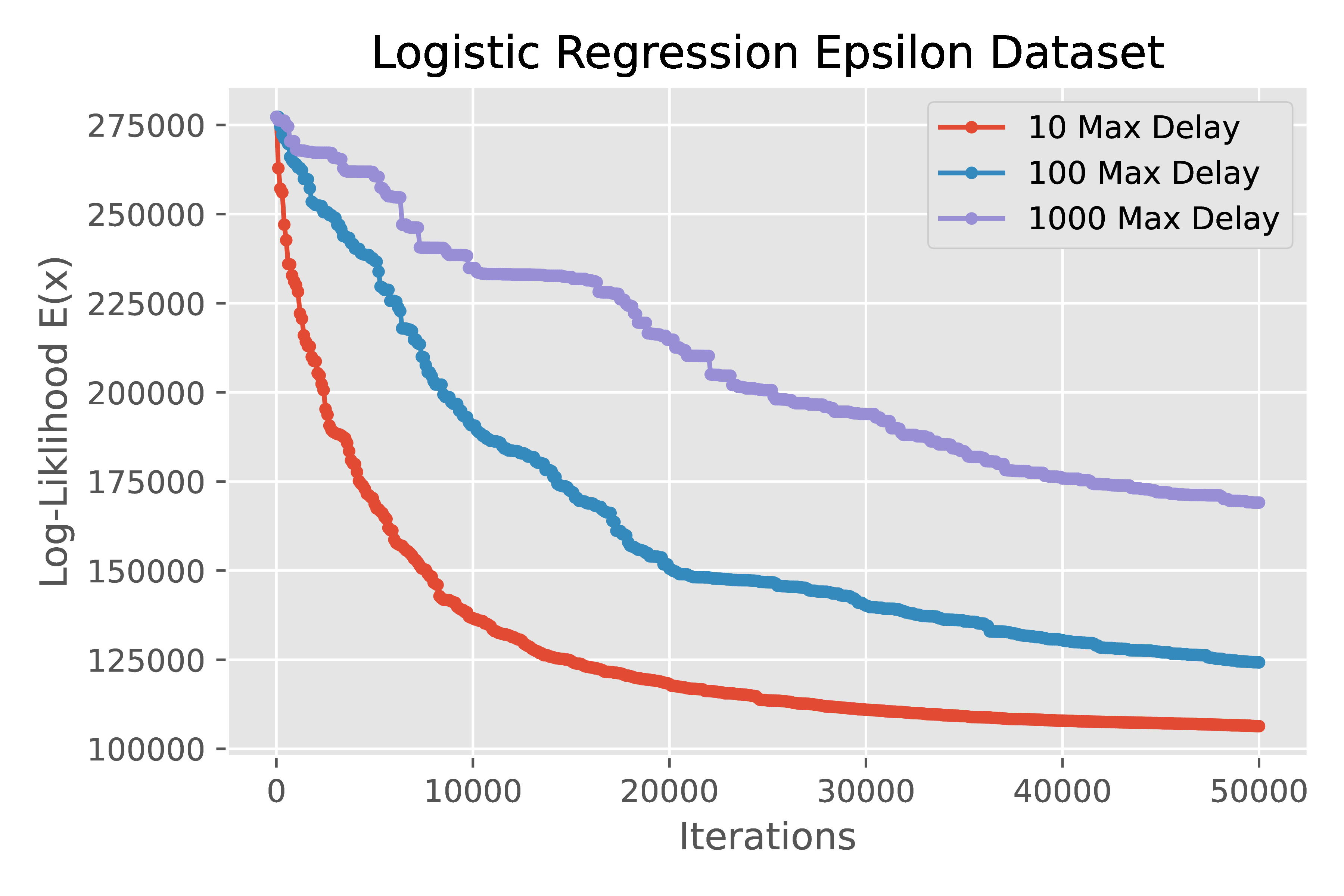
Figure 1: Comparison between the convergence rate of BCD in Algorithm 1 with the maximum delay $B\in\{10,100,1000\}$.

V Conclusions

We derived convergence rates of asynchronous coordinate decent parallelized among $n$ processors for functions satisfying the Polyak-Łojasiewicz (PL) condition and those satisfying the Regularity Condition (RC). Future work includes deriving similar convergence rates for stochastic settings.

VI Appendix

We begin with the following basic lemmas.

Lemma 2.

For all $t\geq 0$ and all $i$, we have ${\left\|x^{i}(t)-x(t)\right\|\leq\gamma\sum_{\tau=t-B}^{t-1}\left\|s(\tau)\right\|.}$

Proof: See Equation (5.9) in [11, Section 7.5]. $\blacksquare$

Next, we quantify the $B$-step decrease in the function value in the true state $x(t)$.

Lemma 3.

For all $t\geq 0$, we have

$$f (x(t+B))-f(x(t))\leq\frac{L}{2}\gamma^{2}nB\sum_{\tau=t-B}^{t-1}\left\|s\left(\tau\right)\right\|^{2}$$

$$+\left(\gamma^{2}L\left(\frac{B}{2}(n+1)+1\right)-\gamma\right)\sum_{\tau=t}^{t+B-1}\|s(\tau)\|^{2}.$$ (14)

Proof: From the Descent Lemma [11, Section 3.2], we have

$$f(x(t+1))=f(x(t)+\gamma s(t))$$

$$\leq f(x(t))+\gamma\sum_{i=1}^{n}s_{i}(t)^{T}\nabla_{i}f(x(t))+L\gamma^{2}\left\|s(t)\right\|^{2}.$$

Adding $(s_{i}(t)-s_{i}(t))$ to $\nabla_{i}f(x(t))$ and applying the Lipschitz property of the gradient gives

$$f(x(t+1))-f(x(t))$$ (15)

$$\leq L\gamma\sum_{i=1}^{n}\left\|\nabla_{i}f(x^{i}(t))\right\|\left\|x(t)-x^{i}(t)\right\|+(L\gamma^{2}-\gamma)\left\|s(t)\right\|^{2}.$$ (16)

Employing Lemma 2, and applying the inequality $ab\leq\frac{1}{2}(a^{2}+b^{2})$ inside the sum, we find

$$f(x(t+1))-f(x(t))$$ (17)

$$\leq\frac{L}{2}\!\gamma^{2}\left[B\left\|s\left(t\right)\right\|^{2}+\!n\!\!\!\sum_{\tau=t-B}^{t-1}\left\|s\left(\tau\right)\right\|^{2}\right]+(L\gamma^{2}-\gamma)\left\|s(t)\right\|^{2}.$$ (18)

The proof is completed by applying this inequality successively to $t,t+1,\dots,t+B-1$, and summing them up. $\blacksquare$

The proof scheme up to this point closely follows [11, 16], which were not focused on PL functions. From this point on, we leverage the $\mu$-PL property of the objective function, and the following lemma and the rest of the results are new. The next lemma bounds the one-step change in $x(t)$.

Lemma 4.

For all $t\geq 0$, there holds

$$\left\|x(t+1)-x(t)\right\|^{2} \leq\left(n^{2}B\gamma^{4}L^{2}+\gamma^{2}Ln\right)\sum_{\tau=t-B}^{t-1}\left\|s\left(\tau\right)\right\|^{2}$$

$$+\left(\gamma^{2}+\gamma^{4}LnB\right)\|\nabla f(x(t))\|^{2}.$$

Proof: With $x(t+1)=x(t)+\gamma s(t)$, we add and subtract $\gamma\nabla f\big{(}x(t)\big{)}$ and apply the triangle inequality to find

$$\|x(t +1)\!-\!x(t)\|\! \leq\|\gamma s(t)+\gamma\nabla f(x(t))\|+\|\gamma\nabla f(x(t))\|.$$

Squaring both sides, we expand to find

$$\|x(t +1)-x(t)\|^{2}\leq\|\gamma\nabla f(x(t))\|^{2}$$ (19)

$$+2\gamma\sum_{i=1}^{n}\|\gamma\nabla f(x(t))\|\left\|s_{i}(t)\!+\!\nabla_{i}f(x(t))\right\|$$ (20)

$$+\gamma^{2}\sum_{i=1}^{n}\|\nabla_{i}f(x(t))+s_{i}(t)\|^{2}.$$ (21)

Using the Lipschitz property of the gradient gives

$$\|x(t\!+\!1)\! -\!x(t)\|^{2}\!\leq\!\|\gamma\nabla f(x(t))\|^{2}\!+\!\gamma^{2}L^{2}\sum_{i=1}^{n}\left\|x^{i}(t)\!-\!x(t)\right\|^{2}$$ (22)

$$+2\gamma L\sum_{i=1}^{n}\|\gamma\nabla f(x(t))\|\|x^{i}(t)-x(t)\|.$$ (23)

Applying Lemma 2, we expand to find

$$\|x(t+1)-x(t)\|^{2}\!\leq n^{2}B\gamma^{4}L^{2}\!\!\!\sum_{\tau=t-B}^{t-1}\!\!\!\left\|s(\tau)\right\|^{2}\!+\!\|\gamma\nabla f(x(t))\|^{2}$$ (24)

$$+\gamma^{2}Ln\sum_{\tau=t-B}^{t-1}\left\|s(\tau)\right\|^{2}+\gamma^{2}LnB\|\gamma\nabla f(x(t))\|^{2},$$ (25)

where we use $(\sum_{i=1}^{K}y_{i})^{2}\leq K\sum_{i=1}^{K}y_{i}^{2}$ and ${ab\leq\frac{1}{2}(a^{2}+b^{2})}$. Rearranging completes the proof. $\hfill\blacksquare$

The next lemma bounds the distance to minima.

Lemma 5.

Take ${\gamma<\min\{\frac{2}{L}\frac{1}{Ln^{2}B+B+1},\frac{1}{L\frac{B}{2}(n+1)+L+\frac{L}{2}nB}\}}$. For all $t\geq 0$, we have

$$f(x(t+B))-f^{*}\leq\left(1-C_{1}\right)\left(f(x(t))-f^{*}\right)\\ +(C_{2}+C_{3})\sum_{\tau=t-B}^{t-1}\left\|s\left(\tau\right)\right\|^{2},$$ (26)

where $C_{1}$, $C_{2}$, and $C_{3}$ are positive constants defined as ${C_{1}=-\mu\left(\gamma^{4}L^{2}nB+\gamma^{2}\left(LB+L\right)-2\gamma\right)}$, ${C_{2}=\frac{1}{2}n^{2}B\gamma^{4}L^{3}+\frac{1}{2}\gamma^{2}L(L+1)n},$ and ${C_{3}:=\frac{L}{2}\gamma^{2}nB}$.

Proof: By Lipschitz continuity (cf. Assumption 1) we write

$$f(x(t+1)) -f(x(t))\leq\langle\nabla f(x(t)),\gamma s(t)\rangle$$

$$+\frac{L}{2}\left\|x(t+1)-x(t)\right\|^{2}$$

$$\leq\gamma L\sum_{i=1}^{n}\left\|x(t)-x^{i}(t)\right\|\left\|\nabla_{i}f(x(t))\right\|$$

$$-\gamma\left\|\nabla f(x(t))\right\|^{2}+\frac{L}{2}\left\|x(t+1)-x(t)\right\|^{2},$$

where we added $\nabla f(x(t))-\nabla f(x(t))$ to $\gamma s(t)$ and used Cauchy-Schwarz and the Lipschitz continuity of the gradient. Next, applying Lemma 2 and then using $ab\leq\frac{1}{2}(a^{2}+b^{2})$ on the first term of the RHS and simplifying we get

$$f(x(t+1))-f(x(t))\leq\frac{L}{2}\left\|x(t+1)-x(t)\right\|^{2}$$

$$+\left(\frac{\gamma^{2}}{2}LB-\gamma\right)\left\|\nabla f(x(t))\right\|^{2}+\frac{\gamma^{2}}{2}Ln\sum_{\tau=t-B}^{t-1}\left\|s(\tau)\right\|^{2}.$$

Applying Lemma 4, we obtain

$$f(x(t+1))-f(x(t))$$

$$\leq\left(\frac{1}{2}nB\gamma^{4}L^{3}+\frac{1}{2}\gamma^{2}L(L+1)n\right)\sum_{\tau=t-B}^{t-1}\left\|s(\tau)\right\|^{2}$$

$$+\left(\frac{1}{2}\gamma^{4}L^{2}n^{2}B+\gamma^{2}\left(\frac{1}{2}LB+\frac{L}{2}\right)-\gamma\right)\left\|\nabla f(x(t))\right\|^{2}.$$

The fact that $\gamma<1$ and the first term in the definition of $\gamma$ ensure that ${\frac{1}{2}\gamma^{4}L^{2}n^{2}B+\gamma^{2}\left(\frac{1}{2}LB+\frac{L}{2}\right)-\gamma\leq 0}$. Using this and the PL inequality, we have

$$f(x(t+1))-f^{*} \leq(1-C_{1})\left(f(x(t))-f^{*}\right)$$ (27)

$$+C_{2}\sum_{\tau=t-B}^{t-1}\left\|s(\tau)\right\|^{2},$$ (28)

where we have also added $-f^{*}$ to both sides. For a small enough $\gamma$, repeating the argument in Lemma 3 from $t+1$ to $t+B$, we find

$$-f(x(t+1))\leq-f(x(t+B))+\frac{L}{2}\gamma^{2}nB\sum_{\tau=t-B}^{t-1}\left\|s\left(\tau\right)\right\|^{2}.$$ (29)

Using (29) in (28), completes the proof. $\blacksquare$

To streamline further analyses, we define ${\alpha(t):=f(x(t))-f^{*},}$ ${\beta(t):=\gamma^{2}\sum_{\tau=t-B}^{t-1}\left\|s(\tau)\right\|^{2}.}$ We next find upper bounds for $\beta(t)$ and $\beta(t-B)$. We substitute $t-B$ for $t$ and $t-2B$ for $t$ consecutively in (14), and by rearranging the terms, we obtain

$$\gamma^{-2}\beta(t)\leq\frac{1}{C_{4}}\left(\alpha(t-B)+\frac{L}{2}nB\beta(t-B)-\alpha(t)\right),$$ (30)

$$\gamma^{-2}\beta(t-B)\leq\frac{1}{C_{4}}\bigg{(}\alpha(t-2B)\\ +\frac{L}{2}nB\beta(t-2B)-\alpha(t-B)\bigg{)},$$ (31)

where ${C_{4}:=\gamma-\gamma^{2}L\left(\frac{B}{2}(n+1)+1\right)}\in\mathbb{R}^{+}$. Next, we employ (30) to bound $\beta(t)$ in Lemma 5, which gives

$$\alpha(t+B)\leq \left(1-C_{1}-\frac{C_{2}+C_{3}}{C_{4}}\right)\alpha(t)+$$ (32)

$$\frac{C_{2}+C_{3}}{C_{4}}\left(\alpha(t-B)+\frac{L}{2}nB\beta(t-B)\right).$$ (33)

Using (31), we bound the term $\beta(t-B)$ in (32), and by simplifying the terms, we obtain

$$\alpha(t+B)\leq\left(1-C_{1}-\frac{C_{2}+C_{3}}{C_{4}}\right)\alpha(t)+\left(\frac{C_{2}+C_{3}}{C_{4}}\right)\cdot$$

$$\biggl{[}(1-\frac{C_{3}}{C_{4}})\alpha(t-B)+\frac{C_{3}}{C_{4}}\alpha(t-2B)+\frac{L}{2}nB\frac{C_{3}}{C_{4}}\beta(t-2B)\biggr{]}.$$ (34)

Next, by applying Lemma 3, at ${t,t+B,t+2B,\dots}$ and summing up those equations, we obtain

$$\alpha(t+kB) \leq\alpha(t)+\left(-C_{4}+C_{3}\right)\sum_{l=1}^{k-1}\sum_{\tau=t+\left(l-1\right)B}^{t+lB-1}\left\|s\left(\tau\right)\right\|^{2}$$ (35)

$$-C_{4}\sum_{\tau=t+\left(k-1\right)B}^{t+kB-1}\|s(\tau)\|^{2}+C_{3}\sum_{\tau=t-B}^{t-1}\left\|s\left(\tau\right)\right\|^{2}.$$ (36)

Using $\gamma<\frac{1}{L\frac{B}{2}(n+1)+L+\frac{L}{2}nB}$ makes $\left(C_{3}-C_{4}\right)<0$, and therefore we get

$$\alpha(t+kB)\leq\alpha(t)+\frac{L}{2}nB\beta(t)$$ (37)

$$\!\!\!+\!\left(L(\frac{B}{2}(n+1)+1)-\gamma^{-1}+\frac{L}{2}nB\right)\beta(t+B).$$ (38)

By the PL inequality, $f(x(t))\geq f^{*}$ for all $x(t)$ and therefore ${\lim\inf_{t\rightarrow\infty}f(x(t))\geq f^{*}}$, which gives ${\alpha(t+kB)\geq 0}$ for all $k$. From this fact and (37) we obtain

$$\beta(t+B)\leq\frac{\alpha(t)+\frac{L}{2}nB\beta(t)}{\gamma^{-1}-L\left(\frac{B}{2}(n+1)+1\right)-\frac{L}{2}nB}.$$ (39)

Finally, using (VI) and (39) we are able to show the main result on asynchronous linear convergence of BCD.

Proof of Theorem 1: For sufficiently small $\gamma$, each step of Algorithm 1 decreases the objective function $f(x)$, e.g., (17). Moreover, since the solution set is finite (from Assumption 1) and $f(x)$ is bounded from below due to the PL inequality, the sequence $\{x(t)\}_{t\in\mathbb{N}}$ generated by Algorithm 1 converges. In particular, it is bounded.

We proceed to show the linear convergence by induction on $k$. Take the scalar $\eta$ large enough such that

$$\alpha(t),\;\alpha(t+B),\;\beta(t),\;\beta(t+B)\leq\eta;$$ (40)

such an $\eta$ exists because $x(t)$ is bounded, and by continuity so are $\alpha(t)$ and $\beta(t)$. Then (7) and (8) hold for $k=0$ and $k=1$. We show that if $\alpha(t+kB)\leq\left(1-\gamma\mu\right)^{k-1}\eta$ and $\beta(t+kB)\leq\left(1-\gamma\mu\right)^{k-1}\eta$, then ${\alpha(t+(k+1)B)\leq\left(1-\gamma\mu\right)^{k}\eta}$ and ${\beta(t+(k+1)B)\leq\left(1-\gamma\mu\right)^{k}\eta}$ for $k\geq 1$. By this induction hypothesis, (VI) is written as

$$\alpha( t+(k+1)B)\leq(1-C_{1}-\frac{C_{2}+C_{3}}{C_{4}})\eta(1-\gamma\mu)^{k-1}$$

$$+\frac{C_{2}+C_{3}}{C_{4}}\Bigg{(}(1-\frac{C_{3}}{C_{4}})\eta(1-\gamma\mu)^{k-2}+\frac{C_{3}}{C_{4}}\eta(1-\gamma\mu)^{k-3}$$

$$+(\frac{L}{2}nB)\frac{C_{3}}{C_{4}}\eta(1-\gamma\mu)^{k-3}\Bigg{)}.$$

Factoring out the term $\left(1-\gamma\mu\right)^{k-1}\eta$, using the inequality $\left(1-\gamma\mu\right)^{-1}<(1+2\gamma\mu)$ and its square, and simplifying the above equation we get

$$\alpha (t\!+\!(k\!+\!1)B)\leq\Biggl{[}1\!-\!C_{1}\!+\!\frac{C_{2}\!+\!C_{3}}{C_{4}}\Biggl{(}\!2\gamma\mu-\frac{C_{3}}{C_{4}}\left(1\!+\!2\gamma\mu\right)$$

$$+\frac{C_{3}}{C_{4}}(1+\frac{L}{2}nB)(1+4\gamma^{2}\mu^{2}+4\gamma\mu)\Biggr{)}\Biggr{]}\eta\left(1-\gamma\mu\right)^{k-1}.$$

Next, take $\gamma<\frac{1}{\mu}$ which gives $1+4\gamma\mu(1+\gamma\mu)<1+8\gamma\mu$. We use that and the inequality, $\left(1-\gamma L\left(\frac{B}{2}(n+1)+1\right)\right)^{-1}<1+2\gamma L\left(\frac{B}{2}(n+1)+1\right)$ and expand to get

$$\alpha(t+(k+1)B)\leq\Biggl{[}1+\mu\left(\gamma^{4}L^{2}nB+\gamma^{2}\left(LB+L\right)-2\gamma\right)$$

$$+(1+2\gamma L(\frac{B}{2}(n+1)+1))\,\cdot$$

$$(\frac{L}{2}\gamma nB+\frac{1}{2}n^{2}B\gamma^{3}L^{3}+\frac{1}{2}\gamma L(L+1)n)\,\cdot$$

$$(2\gamma\mu+\frac{C_{3}}{C_{4}}(\frac{L}{2}nB+8\gamma\mu+LnB4\gamma\mu))\Biggr{]}\eta\left(1-\gamma\mu\right)^{k-1}.$$

Define the constants $A_{1},A_{2}\in\mathbb{R}^{+}$ by $A_{1}:=\frac{L}{2}nB(1+2L(\frac{B}{2}(n+1)+1)),$ $A_{2}:=2\mu+A_{1}\left(\frac{L}{2}nB+4LnB+8\right)$. Note that from $\gamma<1$ we have $\frac{C_{3}}{C_{4}}<\gamma A_{1}$. Simplifying gives

$$\alpha( t+(k+1)B)\leq\Biggl{[}1-2\gamma\mu+\mu\gamma^{2}\left(L^{2}nB+LB+L\right)$$

$$+\gamma^{2}\left(A_{2}+2A_{2}L(\frac{B}{2}(n+1)+1)\right)\cdot$$

$$\left(\frac{L}{2}nB+\frac{1}{2}n^{2}BL^{3}+\frac{1}{2}L(L+1)n\right)\Biggr{]}\eta\left(1-\gamma\mu\right)^{k-1}.$$

Taking $\gamma$ according to

$$\gamma\leq \min\Bigg{\{}\frac{1}{2L}\frac{1}{LnB+B+1},$$

$$\frac{\mu}{A_{2}Ln}\frac{1}{\left(1+L\left(B(n+1)+2\right)\right)\left(nBL^{2}+L+B+1\right)}\Bigg{\}}$$

allows us to upper bound all of the above terms to get

$$\alpha(t+(k+1)B)\leq\left(1-\gamma\mu\right)^{k}\eta.$$ (41)

This completes the first part of the proof. From the induction hypothesis, (39) gives

$$\beta(t+(k+1)B)\leq\frac{\eta\left(1-\gamma\mu\right)^{k-1}+\frac{L}{2}nB\eta\left(1-\gamma\mu\right)^{k-1}}{\left(\gamma^{-1}-L\left(\frac{B}{2}(n+1)+1\right)-\frac{L}{2}nB\right)}.$$ (42)

Taking $\gamma$ according to $\gamma<\frac{1}{L\frac{B}{2}\left(3n+1\right)+L+\mu+1}$ therefore gives

$$\beta(t+(k+1)B)\leq\left(1-\gamma\mu\right)^{k}\eta.$$ (43)

This holds for all $t$. The value of $\gamma_{0}$ can be found by combining the upper bounds on admissible stepsizes $\gamma$ in Lemma 5 and those used above. $\hfill\blacksquare$

References

- [1] X. Lian, Y. Huang, Y. Li, and J. Liu, “Asynchronous parallel stochastic gradient for nonconvex optimization,” in Advances in Neural Information Processing Systems, 2015, pp. 2737–2745.
- [2] K. Bonawitz, H. Eichner, W. Grieskamp, D. Huba, A. Ingerman, V. Ivanov, C. Kiddon, J. Konečný, S. Mazzocchi, B. McMahan, T. Van Overveldt, D. Petrou, D. Ramage, and J. Roselander, “Towards federated learning at scale: System design,” in Proceedings of Machine Learning and Systems, A. Talwalkar, V. Smith, and M. Zaharia, Eds., vol. 1, 2019, pp. 374–388.
- [3] P. Swerling, “Modern state estimation methods from the viewpoint of the method of least squares,” IEEE Transactions on Automatic Control, vol. 16, no. 6, pp. 707–719, 1971.
- [4] K. J. Åström and P. Eykhoff, “System identification—a survey,” Automatica, vol. 7, no. 2, pp. 123–162, 1971.
- [5] B. T. Polyak, “Gradient methods for minimizing functionals,” Zhurnal Vychislitel’noi Matematiki i Matematicheskoi Fiziki, vol. 3, no. 4, pp. 643–653, 1963.
- [6] H. Karimi, J. Nutini, and M. Schmidt, “Linear convergence of gradient and proximal-gradient methods under the polyak-łojasiewicz condition,” in Joint European Conference on Machine Learning and Knowledge Discovery in Databases. Springer, 2016, pp. 795–811.
- [7] X. Yi, S. Zhang, T. Yang, T. Chai, and K. H. Johansson, “A primal-dual sgd algorithm for distributed nonconvex optimization,” arXiv preprint arXiv:2006.03474, 2020.
- [8] F. Haddadpour, M. M. Kamani, M. Mahdavi, and V. Cadambe, “Local sgd with periodic averaging: Tighter analysis and adaptive synchronization,” in Advances in Neural Information Processing Systems, 2019, pp. 11 082–11 094.
- [9] S. U. Stich, “Local sgd converges fast and communicates little,” arXiv preprint arXiv:1805.09767, 2018.
- [10] Z. Peng, Y. Xu, M. Yan, and W. Yin, “Arock: an algorithmic framework for asynchronous parallel coordinate updates,” SIAM Journal on Scientific Computing, vol. 38, no. 5, pp. A2851–A2879, 2016.
- [11] D. P. Bertsekas and J. N. Tsitsiklis, Parallel and distributed computation: numerical methods. Prentice hall Englewood Cliffs, NJ, 1989, vol. 23.
- [12] H. Tang, X. Lian, M. Yan, C. Zhang, and J. Liu, “: Decentralized training over decentralized data,” in Proceedings of the 35th International Conference on Machine Learning, ser. Proceedings of Machine Learning Research, J. Dy and A. Krause, Eds., vol. 80. PMLR, 10–15 Jul 2018, pp. 4848–4856.
- [13] H. Yu and R. Jin, “On the computation and communication complexity of parallel sgd with dynamic batch sizes for stochastic non-convex optimization,” arXiv preprint arXiv:1905.04346, 2019.
- [14] E. J. Candes, X. Li, and M. Soltanolkotabi, “Phase retrieval via wirtinger flow: Theory and algorithms,” IEEE Transactions on Information Theory, vol. 61, no. 4, pp. 1985–2007, 2015.
- [15] Y. Chi, Y. M. Lu, and Y. Chen, “Nonconvex optimization meets low-rank matrix factorization: An overview,” IEEE Transactions on Signal Processing, vol. 67, no. 20, pp. 5239–5269, 2019.
- [16] P. Tseng, “On the rate of convergence of a partially asynchronous gradient projection algorithm,” SIAM Journal on Optimization, vol. 1, no. 4, pp. 603–619, 1991.
- [17] L. Cannelli, F. Facchinei, G. Scutari, and V. Kungurtsev, “Asynchronous optimization over graphs: Linear convergence under error bound conditions,” IEEE Transactions on Automatic Control, 2020.
- [18] Y. Zhou and Y. Liang, “Characterization of gradient dominance and regularity conditions for neural networks,” arXiv preprint arXiv:1710.06910, 2017.
- [19] S. Bhojanapalli, B. Neyshabur, and N. Srebro, “Global optimality of local search for low rank matrix recovery,” in Advances in Neural Information Processing Systems, 2016, pp. 3873–3881.
- [20] C. C. Aggarwal, Linear Algebra and Optimization for Machine Learning. Springer, 2020.