A* Search Without Expansions: Learning Heuristic Functions with Deep Q-Networks

Abstract

Efficiently solving problems with large action spaces using A* search has been of importance to the artificial intelligence community for decades. This is because the computation and memory requirements of A* search grow linearly with the size of the action space. This burden becomes even more apparent when A* search uses a heuristic function learned by computationally expensive function approximators, such as deep neural networks. To address this problem, we introduce Q* search, a search algorithm that uses deep Q-networks to guide search in order to take advantage of the fact that the sum of the transition costs and heuristic values of the children of a node can be computed with a single forward pass through a deep Q-network without explicitly generating those children. This significantly reduces computation time and requires only one node to be generated per iteration. We use Q* search to solve the Rubik’s cube when formulated with a large action space that includes 1872 meta-actions and find that this 157-fold increase in the size of the action space incurs less than a 4-fold increase in computation time and less than a 3-fold increase in number of nodes generated when performing Q* search. Furthermore, Q* search is up to 129 times faster and generates up to 1288 times fewer nodes than A* search. Finally, although obtaining admissible heuristic functions from deep neural networks is an ongoing area of research, we prove that Q* search is guaranteed to find a shortest path given a heuristic function that neither overestimates the cost of a shortest path nor underestimates the transition cost.

1 Introduction

A* Search [13] is a best-first search algorithm guided by a cost function that is the sum of the path cost of a node and the heuristic value of the state associated with that node. The heuristic value is computed by a heuristic function that estimates the cost to go from a given state to the nearest goal state via a shortest path. At every iteration, A* search selects the node with the lowest cost for expansion and computes the cost of all of its children. This process continues until a node associated with a goal state is selected for expansion. Expanding a node requires that every possible action be applied to the state associated with that node, thereby generating new states and, subsequently, new nodes. After a node is generated, the A* search algorithm computes the heuristic value of this newly generated node using the heuristic function. Finally, each newly generated node is then pushed to a priority queue that is prioritized by the cost function. Therefore, for each iteration of A* search, the number of new nodes generated, the number of applications of the heuristic function, and the number of nodes pushed to the priority queue increases linearly with the size of the action space. Furthermore, much of this computation is not necessary as, in general, A* search does not expand every node that it generates.

The need to reduce this linear increase in computational cost has become more relevant with the more frequent use of deep neural networks (DNNs) [25] as heuristic functions. While DNNs are universal function approximators [17], they are computationally expensive when compared to heuristic functions based on domain knowledge, human intuition, and pattern databases [10]. Nonetheless, DNNs are able to learn heuristic functions to solve problems ranging from puzzles [9, 4, 20, 1], to quantum computing [31], to chemical synthesis [8], while making very few assumptions about the structure of the problem. Due to their flexibility and ability to generalize, DNNs offer the promise of learning heuristic functions in a largely domain-independent fashion. Removing the linear increase in computational cost as a function of the size of the action space would make DNNs practical for a wide range of applications with large action spaces, such as multiple sequence alignment, theorem proving, program synthesis, and chemical synthesis.

We introduce Q* search, a search algorithm guided by a deep Q-network (DQN) [21] that requires only one node to be generated per iteration. DQNs are DNNs that map a single state to the sum of the transition cost and the heuristic value for each of its successor states. This allows us to only generate one node per iteration as we can store tuples of nodes and actions in a priority queue whose priority is determined by the DQN. When removing a tuple of a node and action from the queue, we can then generate a new node by applying the action to the state associated with that node. In addition, the number of times the heuristic function must be applied is constant with respect to the size of the action space instead of linear. As a result, the only aspect of Q* search that depends on the action space is pushing a node, along with each of the possible actions that can be applied to it, to the priority queue. This is also more memory efficient than explicitly generating all child nodes as, in our implementation, each action is only an integer. Our theoretical results show that Q* search is guaranteed to find a shortest path given a heuristic function that neither overestimates the cost of a shortest path nor underestimates the transition cost. Our experimental results on the Rubik’s cube, Lights Out, and 35-Pancake puzzle show that Q* search is orders of magnitude faster than A* search and generates orders of magnitude fewer nodes. While these environments have a fixed action space, the Q* search algorithm is agnostic to whether the action space is fixed or dynamic. In the Discussion section, we discuss avenues for future work that use structured prediction to create DQNs that are applicable to variable action spaces.

2 Related Work

Partial expansion A* search (PEA*) [29] was proposed for problems with large action spaces. PEA* first expands a node by generating all of its children, however, it only keeps the children whose cost is below a certain threshold. It then adds a bookkeeping structure to remember the highest cost of the discarded nodes. The intention of PEA* is to save memory, however, the computational requirements do not reduce as every node removed from the priority queue has to be expanded and the heuristic function has to be applied to all of its children. Enhanced partial expansion A* search (EPEA*) [12] uses a domain-dependent operator selection function to only generate a subset of children based on their cost.

Deferred heuristic evaluation [15] has been used to generate only one node per iteration in A* search. This is accomplished by assigning each child node the same heuristic value as its parent node and deferring the evaluation of the child nodes until they are removed from the priority queue. However, this comes at a cost of inaccuracy, especially when the cost-to-go of a child node can be drastically different than that of its parent. We compare to this method in our experiments and show that, in the vast majority of cases, Q* search finds lower cost solutions and does so much faster than deferred heuristic evaluation. Furthermore, in our experiments, deferred heuristic evaluation sometimes runs out of memory due to its inability to prioritize one child node over another.

3 Preliminaries

3.1 Deep Approximate Value Iteration

Value iteration [23] is a dynamic programming algorithm and a central algorithm in reinforcement learning [5, 6, 26] that iteratively improves a cost-to-go function, $J$, that estimates the cost to go to from a given state to the closest goal state via a shortest path. This cost-to-go function can be readily used as a heuristic function for A* search.

In traditional value iteration, $J$ takes the form of a lookup table where the cost-to-go $J(s)$ is stored for each possible state $s$. Value iteration loops through each state $s$ and computes an updated $J^{\prime}(s)$ using the Bellman equation:

$$J^{\prime}(s)=\min_{a}\sum_{s^{\prime}}P^{a}(s,s^{\prime})(g^{a}(s,s^{\prime})+\gamma J(s^{\prime}))$$ (1)

Here $P^{a}(s,s^{\prime})$ is the transition matrix, representing the probability of transitioning from state $s$ to state $s^{\prime}$ by taking action $a$; $g^{a}(s,s^{\prime})$ is the transition cost, the cost associated with transitioning from state $s$ to $s^{\prime}$ by taking action $a$; and $\gamma\in[0,1]$ is the discount factor. The action $a$ is an action in a set of actions $\mathcal{A}$. Value iteration has been shown to converge to the optimal cost-to-go, $j_{*}$ [7]. That is, $j_{*}(s)$ will return the cost of a shortest path to the closest goal state for every state $s$.

In general, for problems solved with A* search, all transitions are deterministic. Therefore, we can simplify Equation 1 as follows:

$$J^{\prime}(s)=\min_{a}(g^{a}(s,A(s,a))+\gamma J(A(s,a)))$$ (2)

where $A(s,a)$ is the state obtained from taking action $a$ in state $s$. In the problems investigated in this paper, all transition costs are 1 and $\gamma$ is set to 1.

However, representing $J$ as a lookup table is too memory intensive for problems with large state spaces. For instance, the Rubik’s cube has $4.3\times 10^{19}$ possible states. Therefore, we turn to approximate value iteration [6] where $J$ is represented as a parameterized function, $\operatorname{\mathit{j_{\theta}}}$, with parameters $\operatorname{\mathit{\theta}}$. We choose to represent $\operatorname{\mathit{j_{\theta}}}$ as a deep neural network (DNN). The parameters $\operatorname{\mathit{\theta}}$ are learned by using stochastic gradient descent to minimize the following loss function:

$$L(\operatorname{\mathit{\theta}})=(\min_{a}(g^{a}(s,A(s,a))+\gamma j_{\operatorname{\mathit{\theta}}^{-}}(A(s,a)))-\operatorname{\mathit{j_{\theta}}})^{2}$$ (3)

Where $\operatorname{\mathit{\theta}}^{-}$ are the parameters for the “target” DNN that is used to compute the updated cost-to-go. Using a target DNN has been shown to result in a more stable training process [21]. The parameters $\operatorname{\mathit{\theta}}^{-}$ are periodically updated to $\operatorname{\mathit{\theta}}$ during training. While we cannot guarantee convergence to $j_{*}$, approximate value iteration has been shown to approximate $j_{*}$ [6]. For the puzzles investigated in this paper, the states used for training $\operatorname{\mathit{j_{\theta}}}$ are generated by randomly scrambling the goal state between 0 and $K$ times. This allows learning to propagate from the goal state to all other states in the training set. This combination of deep neural networks and approximate value iteration is referred to as deep approximate value iteration (DAVI).

3.2 A* Search

A* search [13] is an informed search algorithm which finds a path between a given start state, $s_{0}$, and a closest goal state, $s_{g}$, in a set of goal states. For simplicity, in our search algorithm notation, any given state, $s$, can refer to a state in the state space or a node in the search tree associated with state $s$. The difference is that a node maintains a pointer to its parent as well as the action the parent took so that a path can be recreated. A* search maintains a priority queue, OPEN, from which it iteratively removes and expands the node with the lowest cost and a dictionary, CLOSED, that maps nodes that have already been generated to their path costs. The cost of each node is $f(s)=g(s)+h(s)$, where $g(s)$ is the path cost, which is the sum of transition costs to get from $s_{0}$ to $s$, and $h(s)$ is the heuristic value, the estimated distance between $s$ and the nearest goal state. After a node is expanded, its children that are not already in CLOSED are added to CLOSED and then pushed to OPEN. If a child node $s$ is already in CLOSED, but a less costly path from $s_{0}$ to $s$ has been encountered, then the path cost of $s$ is updated in CLOSED and $s$ is added to OPEN. The algorithm starts with only $s_{0}$ in OPEN and terminates when the node associated with a goal state is removed from OPEN. In this work, the heuristic function is a DNN $\operatorname{\mathit{j_{\theta}}}$. Pseudocode for the A* search algorithm is given in Algorithm 1.

A* search is guaranteed to find a shortest path if the heuristic function is admissible [13]. An admissible heuristic function is a function that never overestimates the cost of a shortest path. While a DNN is not guaranteed to be admissible, obtaining admissible heuristic functions using DNNs is an ongoing area of research [11, 3].

Algorithm 1 A* Search

  Input: starting node $s_{0}$, DNN $\operatorname{\mathit{j_{\theta}}}$

  OPEN $\leftarrow$ priority queue

  CLOSED $\leftarrow$ maps nodes to their path cost

  $g(s_{0})=0$

  $f(s_{0})=g(s_{0})+\operatorname{\mathit{j_{\theta}}}(s_{0})$

  Push $(s_{0},g(s_{0}))$ to OPEN with cost $c_{0}$

  $\textrm{CLOSED}[s_{0}]=g(s_{0})$

  while not $\textrm{IS\_EMPTY}(\textrm{OPEN})$ do

     $(s,g(s))=\textrm{POP(OPEN)}$

     if $\textrm{IS\_GOAL}(s)$ then

        return $\textrm{PATH\_TO\_GOAL}(s)$

     end if

     for $a$ in $0$ to $|\mathcal{A}|$ do

        $s^{\prime}=A(s,a)$

        $g(s^{\prime})=g(s)+g^{a}(s,s^{\prime})$

        if $s^{\prime}$ not in CLOSED or $g(s^{\prime})<\textrm{CLOSED}[s^{\prime}]$ then

           $\textrm{CLOSED}[s^{\prime}]=g(s^{\prime})$

           $f(s^{\prime})=g(s^{\prime})+\operatorname{\mathit{j_{\theta}}}(s^{\prime})$

           Push $(s^{\prime},g(s^{\prime}))$ to OPEN with cost $f(s^{\prime})$

        end if

     end for

  end while

  return failure

Because the learned heuristic function is a DNN, computing heuristic values can make A* search computationally expensive. To alleviate this issue, one can take advantage of the parallelism provided by graphics processing units (GPUs) by expanding the $N$ lowest cost nodes and computing their heuristic values in parallel. Furthermore, even with a computationally cheap and informative heuristic, A* search can be both time and memory intensive. To address this, one can trade potentially more costly solutions for potentially faster runtimes and less memory usage with a variant of A* search called weighted A* search [22]. Weighted A* search computes the cost of each node as $f(s)=\lambda g(s)+h(s)$ where $\lambda\in[0,1]$ is a scalar weighting. This combination of expanding $N$ nodes every iteration and weighting the path cost by $\lambda$ is referred to as batch-weighted A* search (BWAS).

3.3 Q-learning

Instead of learning a function, $\operatorname{\mathit{j_{\theta}}}$, that maps a state, $s$, to its cost-to-go, one can learn a function, $\operatorname{\mathit{q_{\phi}}}$, that maps $s$ to its Q-factors, which is a vector containing $Q(s,a)$ for all actions $a$ [7]. In a deterministic environment, the Q-factor is defined as:

$$Q(s,a)=g^{a}(s,s^{\prime})+\gamma J(s^{\prime})$$ (4)

where $s^{\prime}$ is equal to $A(s,a)$ and $J(s^{\prime})$ can be expressed in terms of $Q$ with $J(s^{\prime})=\min_{a^{\prime}}{Q(s^{\prime},a^{\prime})}$. Learning $Q$ by iteratively updating the left-hand side of (4) toward its right-hand side is known as Q-learning [28]. Like for DAVI, $Q$ is represented as a parameterized function, $\operatorname{\mathit{q_{\phi}}}$, and we choose a deep neural network for $\operatorname{\mathit{q_{\phi}}}$. This is also known as a deep Q-network (DQN) [21]. The architecture of the DQN is constructed such that the input is the state, $s$, and the output is a vector that represents $\operatorname{\mathit{q_{\phi}}}(s,a)$ for all actions $a$. The parameters $\operatorname{\mathit{\phi}}$ are learned using stochastic gradient descent to minimize the loss function:

$$L(\operatorname{\mathit{\phi}})=(g^{a}(s,s^{\prime})+\gamma\min_{a^{\prime}}{q_{\operatorname{\mathit{\phi}}^{-}}(s^{\prime},a^{\prime})}-\operatorname{\mathit{q_{\phi}}}(s,a))^{2}$$ (5)

Just like in DAVI, the parameters $\operatorname{\mathit{\phi}}^{-}$ of the target DNN are periodically updated to $\operatorname{\mathit{\phi}}$ during training.

Similar to value iteration, Q-learning has been shown to converge to the optimal Q-factors, $q_{*}$, in the tabular case [28]. In the approximate case, Q-learning has a computational advantage over DAVI because, while the number of parameters of the DQN grows with the size of the action space, the number of forward passes needed to compute the loss function stays constant for each update. We will show in our results that, in large action spaces, the training time for Q-learning is 127 times faster than DAVI.

4 Methods

4.1 Q* Search

We present Q* search, a search algorithm that builds on A* search to take advantage of DQNs. Q* search uses tuples containing a node and an action, which we will refer to as node_action tuples, to search for a path to the goal. The path cost of a node_action tuple, $(s,a)$, is $g(s)+g^{a}(s,s^{\prime})$ and the heuristic value is $h(s^{\prime})$, where $s^{\prime}$ is equal to $A(s,a)$. Therefore, the cost of a node_action tuple, $f(s,a)$, is $f(s,a)=g(s)+g^{a}(s,s^{\prime})+h(s^{\prime})$. The Q-factor $Q(s,a)$ is equal to $g^{a}(s,s^{\prime})+h(s^{\prime})$. Therefore, using DQNs, the transition cost and cost-to-go of all child nodes can be computed using $\operatorname{\mathit{q_{\phi}}}$ without having to expand $s$.

At every iteration, Q* search pops a node_action tuple, $(s,a)$, from OPEN and creates a new node, $s^{\prime}=A(s,a)$. Instead of expanding $s^{\prime}$, Q* search applies the DQN to $s^{\prime}$ to obtain the sum of the transition cost and the cost-to-go for all of its children. Therefore, we only need a single forward pass through a DNN instead of $|\mathcal{A}|$. Q* search then pushes the new node_action tuples $(s^{\prime}$, $a^{\prime})$ to OPEN for all actions $a^{\prime}$ where the cost is computed by summing the path cost of $s$ and the output of the DQN corresponding to action $a^{\prime}$. In Q* search, the only part that depends on the size of the action space is pushing nodes to OPEN. Unlike A* search, only one node is generated per iteration, regardless of the size of the action space, and the heuristic function only needs to be applied once per iteration. Pseudocode for the Q* search algorithm is given in Algorithm 2.

We also perform Q* in batches of size $N$ and with a weight $\lambda$. We note that the cost of a node_action tuple for the weighted version of Q* is $f(s,a)=\lambda g(s)+g^{a}(s,s^{\prime})+h(s^{\prime})$ where $s^{\prime}$ is equal to $A(s,a)$. However, $\lambda$ should also be applied to the transition cost $g^{a}(s,s^{\prime})$. This does not happen because the transition cost is not computed separately from the cost-to-go. In this work, all the transition costs are the same, therefore, this constant offset does not affect the order in which nodes are generated. However, in future work, this could be remedied by training a DQN that separates the computation of the transition cost and the cost-to-go.

Algorithm 2 Q* Search

  Input: starting state $s_{0}$, DQN $\operatorname{\mathit{q_{\phi}}}$

  OPEN $\leftarrow$ priority queue

  CLOSED $\leftarrow$ maps nodes to their path cost

  $a=\textrm{NO\_OP}$

  $f(s_{0},a_{0})=\min_{a^{\prime}}{q(s_{0},a^{\prime})}$

  $g(s_{0})=0$

  Push $(s_{0},a,g(s_{0}))$ to OPEN with cost $f(s_{0},a_{0})$

  $\textrm{CLOSED}[s_{0}]=g(s_{0})$

  while not $\textrm{IS\_EMPTY}(\textrm{OPEN})$ do

     $(s,a,g(s))=\textrm{POP(OPEN)}$

     $s^{\prime}=A(s,a)$

     if $\textrm{IS\_GOAL}(s^{\prime})$ then

        return $\textrm{PATH\_TO\_GOAL}(s^{\prime})$

     end if

     $g(s^{\prime})=g(s)+g^{a}(s,s^{\prime})$

     if $s^{\prime}$ not in CLOSED or $g(s^{\prime})<\textrm{CLOSED}[s^{\prime}]$ then

        $\textrm{CLOSED}[s^{\prime}]=g(s^{\prime})$

        $\mathbf{q}=\operatorname{\mathit{q_{\phi}}}(s^{\prime},.)$

        for $a^{\prime}$ in $0$ to $|\mathcal{A}|$ do

           $f(s^{\prime},a^{\prime})=g(s^{\prime})+\mathbf{q}[a^{\prime}]$

           Push $(s^{\prime},a^{\prime},g(s^{\prime}))$ to OPEN with cost $f(s^{\prime},a^{\prime})$

        end for

     end if

  end while

  return failure

5 Results

5.1 Theoretical Results

We will show that Q* search is an admissible search algorithm (meaning that it is guaranteed to find a shortest path) if all Q-factors $Q(s,a)$ neither underestimate $g^{a}(s,s^{\prime})$ nor overestimate $g^{a}(s,s^{\prime})+h^{*}(s^{\prime})$, where $s^{\prime}$ is equal to $A(s,a)$ and $h^{*}(s^{\prime})$ is the cost of a shortest path from state $s^{\prime}$ to a closest goal state. We refer to a heuristic function meeting this criteria as q-admissible. This proof is an adaptation for the proof that A* search is an admissible search algorithm [13].

Lemma 1.

Given that all transition costs are greater than zero, for any node $\hat{s}$ that has not been generated and for any shortest path P from the starting node $s_{0}$ to $\hat{s}$, there exists a node_action tuple $(s,a)$ in OPEN where $s^{\prime}=A(s,a)$ and $s^{\prime}$ is on P with a path cost of $g(s^{\prime})=g(s)+g^{a}(s,s^{\prime})$ equal to the cost of a shortest path from $s_{0}$ to $s^{\prime}$.

Proof.

Let D refer to the set of all CLOSED states on any shortest path P from $s_{0}$ to $\hat{s}$. We know that D contains at least one element because the root node, $s_{0}$, is put in CLOSED at the beginning of the search and $s_{0}$ is on all shortest paths from $s_{0}$ to any node $\hat{s}$, given that $\hat{s}$ is reachable from $s_{0}$. Let $s$ be the node with the highest path cost in D. We know that $s$ cannot be equal to $\hat{s}$ because $\hat{s}$ has not yet been generated and $s$ is in CLOSED, which means it must have been generated. Since $s$ is on P and $s$ is not equal to $\hat{s}$, then one of its children must also be on P. Let $s^{\prime}$ be a child of $s$ that is also on P and $a$ be the action that produces $s^{\prime}$ when applied to $s$. The cost of $s^{\prime}$ is $g(s^{\prime})=g(s)+g^{a}(s,s^{\prime})$. Since, for all nodes in CLOSED, all node action tuples are pushed to OPEN and removed only when selected for generating the next node, either $(s,a)$ must be in OPEN or $s^{\prime}$ must be in CLOSED. Since all transition costs are greater than zero $g(s^{\prime})>g(s)$. Therefore, since $s$ is in CLOSED and has the highest path cost of all nodes in D, $s^{\prime}$ cannot be in CLOSED. Therefore, $(s,a)$ must be in OPEN. ∎

Corollary 1.

Given that all transition costs are greater than zero, a q-admissible heuristic function, and that Q* search has not yet terminated, for any shortest path P from the starting node $s_{0}$ to any goal node $s_{g}$, there exists a node_action tuple $(s,a)$ in OPEN where $s^{\prime}=A(s,a)$ has not been generated and is on P with cost $f(s,a)<=h^{*}(s_{0})$.

Proof.

Since search has not terminated, then we have not yet generated goal node $s_{g}$. Therefore, by Lemma 1, there exists a node_action tuple $(s,a)$ in OPEN where $s^{\prime}=A(s,a)$ is on a shortest path P from $s_{0}$ to $s_{g}$ with a path cost $g(s^{\prime})=g(s)+g^{a}(s,s^{\prime})$ that is equal to the cost of shortest path from $s_{0}$ to $s^{\prime}$. Since we are given a q-admissible heuristic, $q(s,a)$ does not overestimate $g^{a}(s,s^{\prime})+h^{*}(s^{\prime})$. Therefore, $f(s,a)=g(s)+q(s,a)<=g(s)+g^{a}(s,s^{\prime})+h^{*}(s^{\prime})=h^{*}(s_{0})$ ∎

Theorem 1.

Given that all transition costs are greater than zero and a q-admissible heuristic function then Q* search is admissible.

Proof.

Assume the contrary, that Q* terminates at a node_action tuple $(\hat{s},\hat{a})$ where $\hat{s}^{\prime}=A(\hat{s},\hat{a})$ is a goal node with a path cost $g(\hat{s}^{\prime})=g(\hat{s})+g^{\hat{a}}(\hat{s},\hat{s}^{\prime})>h^{*}(s_{0})$. However, Corollary 1 states that, at the time of termination, there was a node_action tuple $(s,a)$ in OPEN and $f(s,a)\leq h^{*}(s_{0})<g(\hat{s}^{\prime})$. We also know that, before $(\hat{s},\hat{a})$ was removed from OPEN, $f(\hat{s},\hat{a})=g(\hat{s}^{\prime})>f(s,a)$ since a q-admissible heuristic function would neither underestimate the transition cost $g^{\hat{a}}(\hat{s},\hat{s}^{\prime})$ nor overestimate the cost-to-go of $\hat{s^{\prime}}$, which is zero. Therefore, Q* search would have removed a node with a cost of, at most, $f(s,a)$, which is less than $f(\hat{s},\hat{a})$, leading to a contradiction. ∎

5.2 Experimental Results

The Rubik’s cube action space has 12 different actions: each of the six faces can be turned clockwise or counterclockwise. We refer to this action space as RC(12). To determine how well Q* can find solutions in large action spaces, we add meta-actions to the Rubik’s cube action space, creating RC(156) and RC(1884). RC(156) has all the actions in RC(12) plus all combinations of actions of size two (144). RC(1884) has all the actions in RC(156) plus all combinations of actions of size three (1728). To ensure none of these additional meta-actions are redundant, the cost for all meta-actions is also set to one. We also test our method on the 7 by 7 Lights Out puzzle [1], which has 49 actions, as well as the 35-Pancake puzzle, which has 35 actions. The machines we use for training and search have 48 2.4 GHz Intel Xeon central processing units (CPUs), 192 GB of random access memory, and two 32GB NVIDIA V100 GPUs.

We train the cost-to-go function with the same architecture described in Agostinelli et al. [1], which has a fully connected layer of size 5,000, followed by another fully connected layer of size 1,000, followed by four fully connected residual blocks of size 1,000 with two hidden layers per residual block [14], followed by a layer of size 1 representing the cost-to-go. The DQN also has the same architecture with the exception that the output layer is a vector that estimates the cost-to-go for taking every possible action. For generating training states, the number of times we scramble the puzzle, $K$, is set to 30 for the Rubik’s cube, 50 for Lights Out, and 70 for the 35-Pancake puzzle. For Q-learning, we select actions according to a Boltzmann distribution where each action $a$ is selected with probability:

$$p_{s,a}=\frac{e^{(\operatorname{\mathit{q_{\phi}}}(s,a)/T)}}{\sum_{a^{\prime}=1}^{|\mathcal{A}|}e^{(\operatorname{\mathit{q_{\phi}}}(s,a^{\prime})/T)}}$$ (6)

where we set the temperature $T=\frac{1}{3}$.

We train with a batch size of 10,000 for 1.2 million iterations using the ADAM optimizer [18]. We update the target networks with the same schedule defined in the DeepCubeA source code [2]. However, as the size of the action space increases, training becomes infeasible for DAVI. Table 1 shows that DAVI would take over a month to train on RC(156) and almost a year to train on RC(1884). Therefore, we reduce the batch size in proportion to the differences in the size of the action space with RC(12). Since RC(156) has 13 times more actions, we train DAVI with a batch size of 769 and since RC(1884) has 157 times more actions, we train DAVI with a batch size of 63. We train with a batch size of 10,000 for both Lights Out and the 35-Pancake puzzle for both DAVI and Q-learning.

We compare to both A* search as well as the deferred version of A* search [15], which we refer to as A_d*, where the heuristic value of each child is set to be the same as the heuristic value of the parent. While this only generates one node per iteration, it introduces inefficiencies because it cannot prioritize one child node over another. In fact, for RC(1884), A_d* was unable to find a solution due to running out of memory. When solving with A* and A_d*, we use the heuristic function computed by DAVI and when solving with Q*, we use the DQN computed by Q-learning.

Table 1: The table shows the number of training iterations per second with a batch size of 10,000 and the projected number of days to train for 1.2 million iterations. DAVI is significantly slower than Q-learning, especially when the size of the action space is large.

Puzzle	Method	Itrs/Sec	Train Time
RC(12)	DAVI	3.96	3.5d
	Q-learning	8.55	1.6d
RC(156)	DAVI	0.42	33d
	Q-learning	7.46	1.9d
RC(1884)	DAVI	0.04	347d
	Q-learning	5.08	2.7d

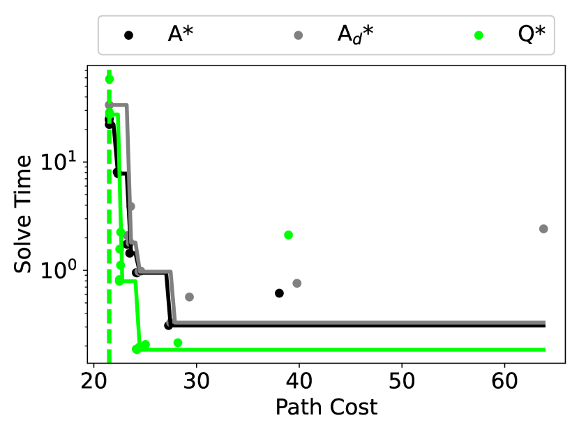
(a) RC(12)

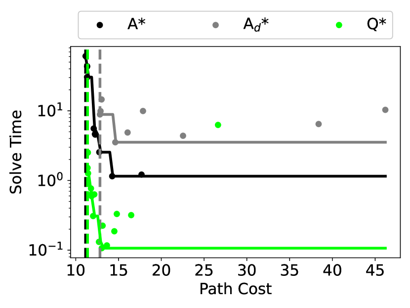
(b) RC(156)

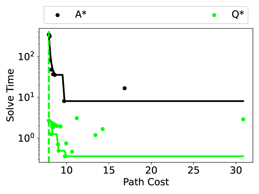
(c) RC(1884)

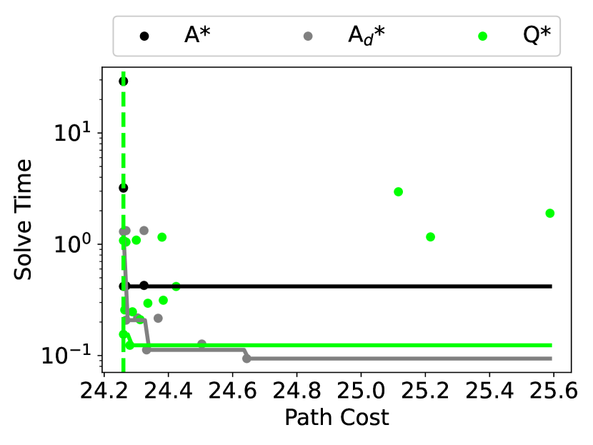
(d) Lights Out

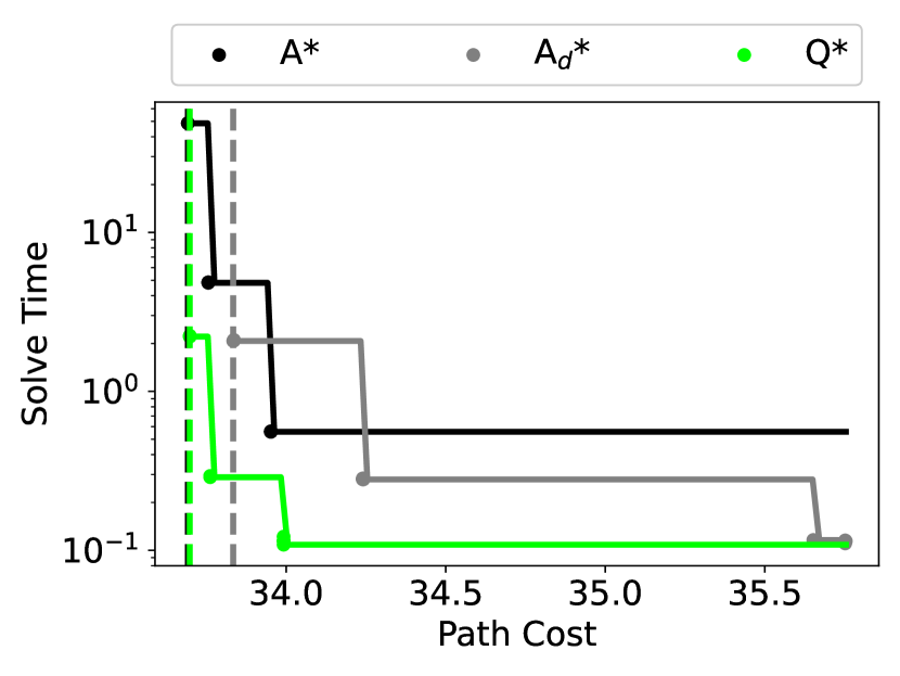
(e) 35-pancake

Figure 1: The figures shows the relationship between the average path cost and the average time to find a solution. The y-axis has a logarithmic scale. Each dot represents a search parameter setting. The dashed line represents the lowest average path cost found. The solid line represents the fastest solution time as a function of a hypothetical threshold for an acceptable average path cost. For RC(1884), A_d* ran out of memory. For almost all thresholds, Q* is significantly faster than A* and A_d*.

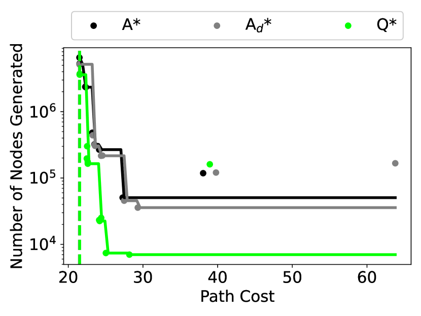
(a) RC(12)

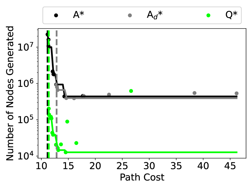
(b) RC(156)

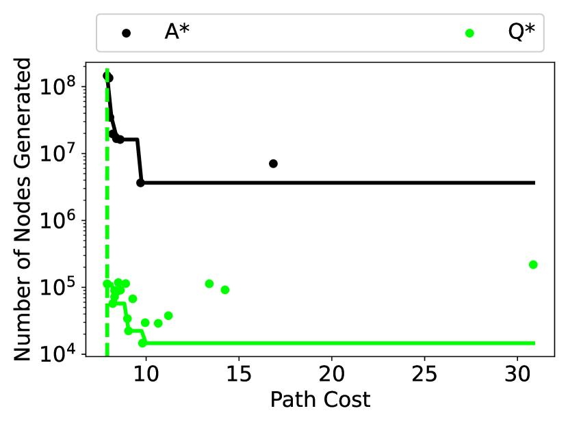
(c) RC(1884)

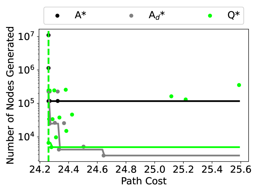
(d) Lights Out

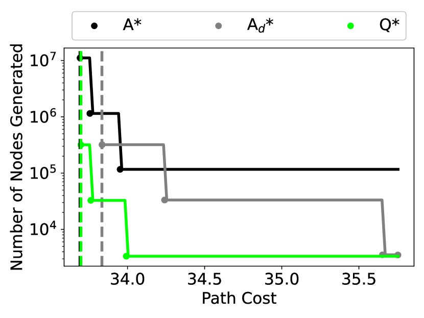
(e) 35-Pancake

Figure 2: The figures shows the relationship between the average path cost and the average number of nodes generated. The y-axis has a logarithmic scale. Each dot represents a search parameter setting. The dashed line represents the lowest average path cost found. The solid line represents the fewest number of nodes generated as a function of a hypothetical threshold for an acceptable average path cost. For RC(1884), A_d* ran out of memory. For almost all thresholds, Q* generates significantly fewer nodes than A* and A_d*.

Table 2: The ratio between A* and Q* search for the solution time and number of nodes generated for hypothetical acceptable path cost thresholds for RC(12), RC(156), and RC(1884). Q* outperforms A* in all instances but one. In the most extreme case, Q* search is 129 times faster and produces 1288 times fewer nodes than A* search.

	Path Cost Threshold
	RC (12)				RC (156)				RC (1884)
	22	25	28		12	14	16		8	9	10
Time	0.8	5.1	1.7		50.8	23.9	10.8		129.7	28.5	22.6
Nodes	1.4	11.9	6.8		92.0	64.0	34.5		1288.4	282.8	249.1

Table 3: The table shows each puzzle with an action space augmented with meta-actions along with the ratio between the size of the action space and the size of the action space for RC(12). It then shows the ratio for the time and number of nodes generated for each method when compared to its own performance on RC(12) averaged over all search parameter settings with the standard deviation in parenthesis. Q* has much better performance for both metrics. For RC(156) Q* finds solutions in even less time than it did for RC(12) due to the addition of meta-actions.

Puzzle	Actions	Method	Time	Nodes Gen
RC(156)	x13	A*	3.5(1.6)	8.7(2.2)
		Q*	0.9(0.7)	1.4(1.3)
RC(1884)	x157	A*	37.0(6.5)	62.7(5.2)
		Q*	3.7(4.0)	2.3(3.6)

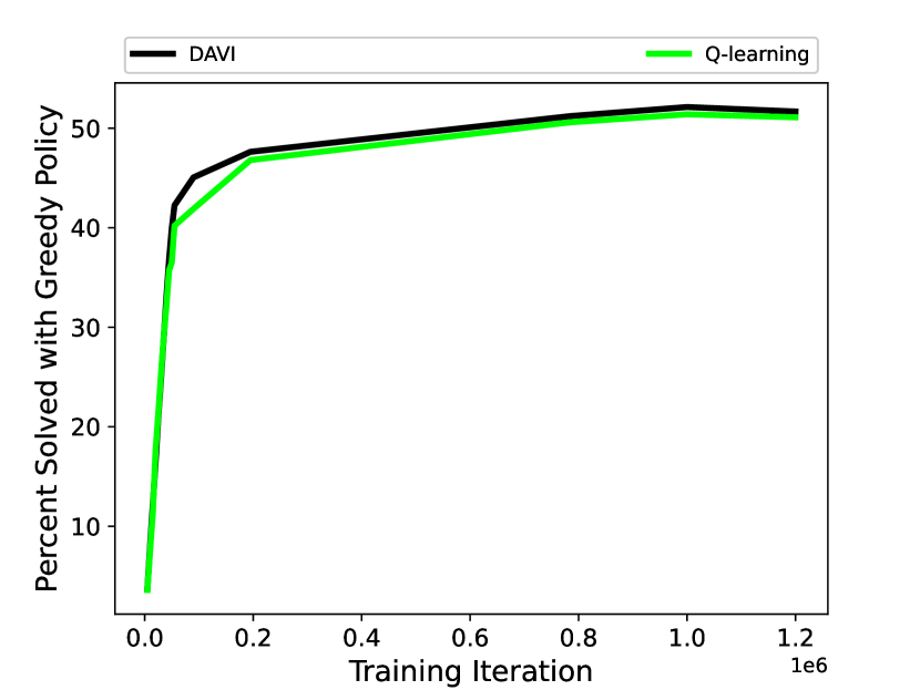
(a) RC(12)

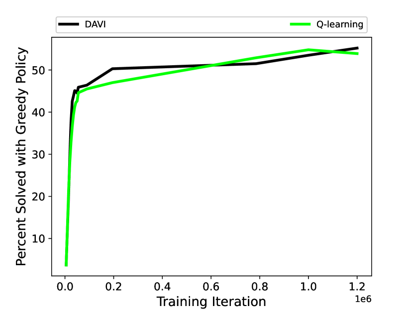
(b) RC(156)

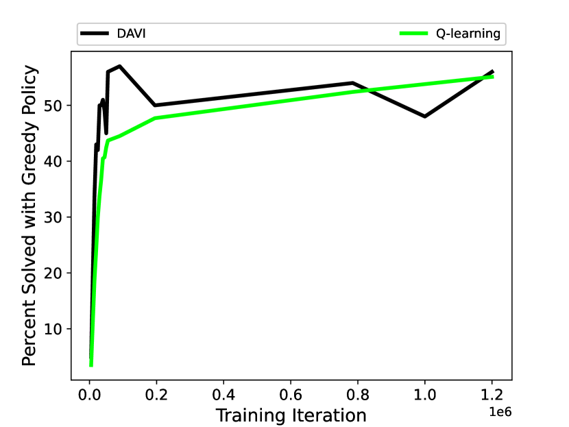
(c) RC(1884)

Figure 3: Percentage of training states solved with a greedy policy as a function of training iteration.

5.2.1 Performance During Search

Prior work on solving the Rubik’s cube with deep reinforcement learning and A* search used $\lambda=0.6$ and $N=10000$ for BWAS [1]. However, since these search parameters create a tradeoff between speed, memory usage, and path cost, we also examine the performance with different parameter settings to understand how A* search and Q* search compare along these dimensions. Therefore, we try all combinations of $\lambda\in\{0.0,0.2,0.4,0.6,0.8,1.0\}$ and $N\in\{100,1000,10000\}$. For each method and each action space, we prune all combinations that cause our machine to run out of memory or that require over 24 hours to complete. We use the same 1,000 test states used for the Rubik’s cube and 500 test states for Lights Out as used in previous work by Agostinelli et al. [1]. We generated 500 test states for the 35-Pancake puzzle. Each test state was obtained by scrambling the puzzle between 1,000 and 10,000. Due to the increase in solving time from A* search, for RC(156), we use a subset of 100 states and for RC(1884), we use a subset of 20 states. We examine the results both in terms of the lowest path cost averaged over all the test states as well as hypothetical cases where there is some threshold for an acceptable average path cost.

For RC(12), the lowest average path cost that A* finds is 21.493 while for Q* it is 21.529. For RC(156), the lowest average path cost that A* finds is 11.15 while for Q* it is 11.38. For RC(1884), the lowest average path cost for both A* and Q* is 7.9. The average path cost becomes smaller as the size of the action space increases because the additional meta-actions allow the Rubik’s cube to be solved in fewer moves. For Lights Out, the lowest average path cost that both A* and Q* find is both 24.6. For the 35-Pancake puzzle, the lowest average path cost that A* finds is 33.692 while for Q* it is 33.698. We obtain information about shortest paths (solutions with the smallest possible path cost) for RC(12) and Lights Out from previous work on DeepCubeA [1]. For RC(12), in the best case, A* finds a shortest path 59% of the time while Q* finds a shortest path 56.4% of the time. For Lights Out, in the best case, both A* and Q* find a shortest path 100% of the time.

The results show that, as the size of the action space increases, the speed and memory advantages of Q* search becomes significant. The memory requirements of the search methods is proportional to the number of nodes generated. In Figure 1, we can see the relationship between the average path cost and the time to find a solution for all search parameter settings. In Figure 2, we can see the relationship between the average path cost and the number of nodes generated for all search parameter settings. The figures show that, for almost any possible path cost threshold, Q* is significantly faster and generates significantly fewer nodes than both A* and A_d*. In the most extreme case, the cheapest average path cost for A* and Q* is identical for RC(1884), however, Q* is 129 times faster and generates 1228 times fewer nodes than A*. These ratios for different desired average path costs are shown in Table 2. The table shows that Q* is often orders of magnitude faster and more memory efficient than A*.

When comparing A* and Q* to themselves for different action spaces, Table 3 shows that, though RC(1884) has 157 times more actions than RC(12), Q* only takes 3.7 times as long to find a solution and generates only 2.3 times as many nodes. On the other hand, in this same scenario, A* takes 37 times as long and generates 62.7 times as many nodes.

5.2.2 Performance During Training

To monitor performance during training, we track the percentage of states that are solved by simply behaving greedily with respect to the cost-to-go function. We generate these states the same way we generate the training states. Figure 3 shows this metric as a function of training time. The results show that, in the case of RC(12), DAVI is slightly better than Q-learning. In RC(156) and RC(1884), even though the batch size for DAVI is smaller, the performance is on par with Q-learning. This may be due to the fact that DAVI is only learning the cost-to-go for a single state while Q-learning must learn the sum of the transition cost and cost-to-go for all possible next states.

6 Discussion

As the size of the action space increases, Q* becomes significantly more effective than A* in terms of solution time and the number of nodes generated. In the largest action space Q* is orders of magnitude faster and generates orders of magnitude fewer nodes than A* while finding solutions with the same average path cost. For smaller action spaces, while Q* is almost always faster and more memory efficient, A* is capable of finding solutions that are slightly cheaper than Q*. This could be due to the difference in what $\operatorname{\mathit{j_{\theta}}}$ and $\operatorname{\mathit{q_{\phi}}}$ are computing. Since the forward pass performed by the DQN, $\operatorname{\mathit{q_{\phi}}}$, is the same as doing a one-step lookahead with $\operatorname{\mathit{j_{\theta}}}$, this could make learning $\operatorname{\mathit{q_{\phi}}}$ more difficult than learning $\operatorname{\mathit{j_{\theta}}}$. This may explain why, in the case of Lights Out, A_d* is, in some cases, faster and generates fewer nodes than Q*. However, Q* becomes better as the path cost threshold decreases. Since training and search are significantly faster for Q-learning and Q*, this gap could be closed with longer training times and searching with larger values of $\lambda$ or $N$.

While the DQN used in this work was for fixed action spaces, Q* search can readily be applied to a dynamic action space given a DQN capable of computing Q-factors for such an action space. Therefore, it is possible to use Q* to solve problems with dynamic action spaces by choosing a DQN architecture that uses structured prediction. Architectures such as graph convolutional policy networks [30], which were used for molecular optimization, could be modified to estimate Q-factors on problems with a graph structure that corresponds to the action space. In problems involving sequences, Long Short-Term Memory [16] or Transformer [27] architectures could be used to compute Q-factors. This would have a direct application to problems with large, but variable, action spaces such as chemical synthesis, theorem proving, program synthesis, and web navigation.

7 Conclusion

Efficiently solving search problems with large action spaces has been of importance to the artificial intelligence community for decades [24, 19, 29]. Q* search uses a DQN to eliminate the majority of the computational and memory burden associated with large action spaces by generating only one node per iteration and requiring only one application of the heuristic function per iteration. When compared to A* search, Q* search is up to 129 times faster and generates up to 1288 times fewer nodes. When increasing the size of the action space by 157 times, Q* search only takes 3.7 times as long and generates only 2.3 times more nodes. The ability that Q* has to efficiently scale up to large action spaces could play a significant role in finding solutions to many important problems with large action spaces.

References

- Agostinelli et al. [2019] Forest Agostinelli, Stephen McAleer, Alexander Shmakov, and Pierre Baldi. Solving the Rubik’s cube with deep reinforcement learning and search. Nature Machine Intelligence, 1(8):356–363, 2019.
- Agostinelli et al. [2020] Forest Agostinelli, Stephen McAleer, Alexander Shmakov, and Pierre Baldi. DeepcubeA. https://github.com/forestagostinelli/DeepCubeA, 2020.
- Agostinelli et al. [2021] Forest Agostinelli, Stephen McAleer, Alexander Shmakov, Roy Fox, Marco Valtorta, Biplav Srivastava, and Pierre Baldi. Obtaining approximately admissible heuristic functions through deep reinforcement learning and A* search. In International Conference on Automated Planning and Scheduling - Bridging the Gap Between AI Planning and Reinforcement Learning Workshop, 2021.
- Arfaee et al. [2011] Shahab Jabbari Arfaee, Sandra Zilles, and Robert C Holte. Learning heuristic functions for large state spaces. Artificial Intelligence, 175(16-17):2075–2098, 2011.
- Bellman [1957] Richard Bellman. Dynamic Programming. Princeton University Press, 1957.
- Bertsekas and Tsitsiklis [1996] Dimitri P Bertsekas and John N Tsitsiklis. Neuro-dynamic programming. Athena Scientific, 1996. ISBN 1-886529-10-8.
- Bertsekas et al. [1995] Dimitri P Bertsekas, Dimitri P Bertsekas, Dimitri P Bertsekas, and Dimitri P Bertsekas. Dynamic programming and optimal control, volume 1. Athena scientific Belmont, MA, 1995.
- Chen et al. [2020] Binghong Chen, Chengtao Li, Hanjun Dai, and Le Song. Retro*: learning retrosynthetic planning with neural guided A* search. In International Conference on Machine Learning, pages 1608–1616. PMLR, 2020.
- Chen and Wei [2011] Hung-Che Chen and Jyh-Da Wei. Using neural networks for evaluation in heuristic search algorithm. In Twenty-Fifth AAAI Conference on Artificial Intelligence, 2011.
- Culberson and Schaeffer [1998] Joseph C Culberson and Jonathan Schaeffer. Pattern databases. Computational Intelligence, 14(3):318–334, 1998.
- Ernandes and Gori [2004] Marco Ernandes and Marco Gori. Likely-admissible and sub-symbolic heuristics. In Proceedings of the 16th European Conference on Artificial Intelligence, pages 613–617. Citeseer, 2004.
- Felner et al. [2012] Ariel Felner, Meir Goldenberg, Guni Sharon, Roni Stern, Tal Beja, Nathan Sturtevant, Jonathan Schaeffer, and Robert Holte. Partial-expansion A* with selective node generation. In Proceedings of the AAAI Conference on Artificial Intelligence, volume 26, 2012.
- Hart et al. [1968] Peter E Hart, Nils J Nilsson, and Bertram Raphael. A formal basis for the heuristic determination of minimum cost paths. IEEE transactions on Systems Science and Cybernetics, 4(2):100–107, 1968.
- He et al. [2016] Kaiming He, Xiangyu Zhang, Shaoqing Ren, and Jian Sun. Deep residual learning for image recognition. In Proceedings of the IEEE conference on computer vision and pattern recognition, pages 770–778, 2016.
- Helmert [2006] Malte Helmert. The fast downward planning system. Journal of Artificial Intelligence Research, 26:191–246, 2006.
- Hochreiter and Schmidhuber [1997] Sepp Hochreiter and Jürgen Schmidhuber. Long short-term memory. Neural computation, 9(8):1735–1780, 1997.
- Hornik et al. [1989] Kurt Hornik, Maxwell Stinchcombe, and Halbert White. Multilayer feedforward networks are universal approximators. Neural networks, 2(5):359–366, 1989.
- Kingma and Ba [2014] Diederik P Kingma and Jimmy Ba. Adam: A method for stochastic optimization. arXiv preprint arXiv:1412.6980, 2014.
- Korf [1993] Richard E Korf. Linear-space best-first search. Artificial Intelligence, 62(1):41–78, 1993.
- McAleer et al. [2019] Stephen McAleer, Forest Agostinelli, Alexander Shmakov, and Pierre Baldi. Solving the Rubik’s cube with approximate policy iteration. In International Conference on Learning Representations, 2019.
- Mnih et al. [2015] Volodymyr Mnih, Koray Kavukcuoglu, David Silver, Andrei A Rusu, Joel Veness, Marc G Bellemare, Alex Graves, Martin Riedmiller, Andreas K Fidjeland, Georg Ostrovski, et al. Human-level control through deep reinforcement learning. Nature, 518(7540):529–533, 2015.
- Pohl [1970] Ira Pohl. Heuristic search viewed as path finding in a graph. Artificial intelligence, 1(3-4):193–204, 1970.
- Puterman and Shin [1978] Martin L Puterman and Moon Chirl Shin. Modified policy iteration algorithms for discounted markov decision problems. Management Science, 24(11):1127–1137, 1978.
- Russell [1992] Stuart J Russell. Efficient memory-bounded search methods. In ECAI, volume 92, pages 1–5, 1992.
- Schmidhuber [2015] Jürgen Schmidhuber. Deep learning in neural networks: An overview. Neural networks, 61:85–117, 2015.
- Sutton and Barto [1998] Richard S Sutton and Andrew G Barto. Reinforcement learning: An introduction, volume 1. MIT press Cambridge, 1998.
- Vaswani et al. [2017] Ashish Vaswani, Noam Shazeer, Niki Parmar, Jakob Uszkoreit, Llion Jones, Aidan N Gomez, Lukasz Kaiser, and Illia Polosukhin. Attention is all you need. arXiv preprint arXiv:1706.03762, 2017.
- Watkins and Dayan [1992] Christopher JCH Watkins and Peter Dayan. Q-learning. Machine learning, 8(3-4):279–292, 1992.
- Yoshizumi et al. [2000] Takayuki Yoshizumi, Teruhisa Miura, and Toru Ishida. A* with partial expansion for large branching factor problems. In AAAI/IAAI, pages 923–929, 2000.
- You et al. [2018] Jiaxuan You, Bowen Liu, Rex Ying, Vijay Pande, and Jure Leskovec. Graph convolutional policy network for goal-directed molecular graph generation. arXiv preprint arXiv:1806.02473, 2018.
- Zhang et al. [2020] Yuan-Hang Zhang, Pei-Lin Zheng, Yi Zhang, and Dong-Ling Deng. Topological quantum compiling with reinforcement learning. Physical Review Letters, 125(17):170501, 2020.