Lifshitz theory of wetting films at three phase coexistence:
The case of ice nucleation on Silver Iodide (AgI)

Abstract

Hypothesis:

As a fluid approaches three phase coexistence, adsorption may take place by the successive formation of two intervening wetting films. The equilibrium thickness of these wetting layers is the result of a delicate balance of intermolecular forces, as dictated by an underlying interface potential. The van der Waals forces for the two variable adsorption layers may be formulated exactly from Dzyaloshinskii-Lifshitz-Pitaevskii theory, and analytical approximations may be derived that extent well beyond the validity of conventional Hamaker theory.

Calculations:

We consider the adsorption equilibrium of water vapor on Silver Iodide where both ice and a water layers can form simultaneously and compete for the vapor as the triple point is approached. We perform numerical calculations of Lifshitz theory for this complex system and work out analytical approximations which provide quantitative agreement with the numerical results.

Findings

At the three phase contact line between AgI/water/air, surface forces promote growth of ice both on the AgI/air and the water/vapor interfaces, lending support to a contact nucleation mode of AgI in the atmosphere. Our approach provides a framework for the description of adsorption at three phase coexistence, and allows for the study of ice nucleation efficiency on atmospheric aerosols.

I Introduction

The preferential adsorption of gases and liquids on an inert solid substrate is ubiquitous in colloidal science, and is often accompanied by the formation of thick wetting films that span from a few nanometers to several microns as two phase coexistence is approached derjaguin87 ; degennes04 ; israelachvili11 ; schick90 . The behavior of the equilibrium layer formed can be fully characterized by an interface potential, $g(h)$, which measures the free energy as a function of the film thickness, $h$ dietrich88 ; schick90 ; degennes04 ; henderson05 . For thick films, $g(h)$ is often dominated by long range van der Waals forces that can be described rigorously with the celebrated Dzyaloshinskii-Lifshitz-Pitaevskii (DLP) theory dzyaloshinskii61 .

A more complex situation arises when the adsorbed wetting film can further segregate and form a new layer between the solid substrate and the mother phase as three phase coexistence is approached takeya06 ; aspenes10 ; nakane19 ; bostrom19 ; antonov14 ; rafai07 ; hartlein08 . This can be quite generally the case for substrates in contact with multicomponent mixtures. Examples include the industrially relevant formation of clathrate hydrates from aqueous solutions of oil or carbon dioxide takeya06 ; aspenes10 ; nakane19 ; bostrom19 , biologically relevant aqueous solutions of Dextran and Bovine Serum Albumin antonov14 ; or theoretically relevant model solutions such as ethanol/n-alkane or lutidine/water mixtures rafai07 ; hartlein08 . The wetting problem now becomes considerably more complex, as the system can exhibit two thick layers of size, say, $l$ and $d$, respectively, that are bounded by the substrate and the mother phase and can feed one from the other depending on the prevailing thermodynamic conditions.

In practice, this complex scenario can be realized for a very relevant one component test system, namely, atmospheric supercooled water vapor in close proximity to the triple point dash06 . As ice nucleates on the surface of inorganic aerosols, the resulting ice/water vapor interface is exposed. This surface is actually a complex system exhibiting a thin premelted water layer, usually referred as Quasi-Liquid Layer (QLL). Its properties largely condition several phenomena related to ice, such as the electrification of storm clouds, frost and snowflakes formation, or ice skating (rosenberg05, ; dash06, ; slater19, ; nagata19, ). Hereby the surface Van der Waals forces play a crucial role in the stabilization of a thick QLL(elbaum91b, ; fiedler20, ).

On the other hand, silver iodide may be used as a nucleus for ice formation(vonnegut47, ), with applications in cloud seeding to induce rainfall over wide areas. The conventional belief was that the capability of the AgI to influence the growth of ice was connected to their lattice match. Nonetheless, recent studies(marcolli16, ) have found substances with similar structures that do not promote nucleation. Thus they relate the faculty of the AgI to serve as ice nucleating agent to the charge distribution in the substrate fraux14 ; zielke15 ; glatz16 . The present work aims at elucidating the role of Van der Waals forces in the ice nucleating activity of silver iodide, by describing precisely the Van der Waals interactions in the framework of the Lifshitz theory, applied to the AgI - Ice - Liquid Water - Air system (Fig. 1).

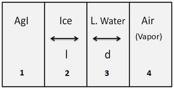
Figure 1: Geometry of layered planar systems studied in this work. An inert substrate, AgI, in contact with water vapor (air), close to three phase coexistence can exhibit intervening phases of ice, with thickness $l$ and water, with thickness $d$. Since the system is subject to material equilibrium each phase feeds from the other. The equilibrium layer thickness of $l$ and $d$ are dictated by the bulk free energies and the interface potential. For the sake of generality and conciseness of notation, we denote the phases AgI, ice, water, air as ’1’, ’2’, ’3’, ’4’, respectively.

The conventional view is that the van der Waals interactions between two surfaces result from the summation of forces between pairs of particles. The interaction coefficients are then added into the Hamaker coefficient, $A_{Ham}$, and the interaction for a layered planar system provides an energy $A_{Ham}/(12\pi h^{2})$, being $h$ the distance between the interacting media israelachvili11 . The Lifshitz theory of the Van der Waals forces goes beyond the pairwise summation, by treating the Van der Waals forces through continuum thermodynamic properties of the polarizable interacting media(parsegian05, ). As a particularly significant result of the detailed electromagnetic treatment, there appears a range of distances where the leading order interactions become retarded and decay as $1/h^{3}$. Accordingly, the effective interaction coefficient itself, $A_{Ham}$, is no longer a constant, but becomes a function of the film thickness as well. Then the generalized expression for the Van der Waals free energy becomes(parsegian05, ):

$$g_{VdW}(h)=-\frac{A_{Ham}(h)}{12\pi h^{2}}$$ (1)

In the study of ice growing at the AgI/air interface, the simple description based on interactions between AgI and air across ice is not valid. Because of the existence of premelting, we also expect the formation of a fourth layer of water in between ice and air. The extension of Lifshitz theory to four media of which one is variable has been known for a long time (ninham70c, ; podgornik03, ; parsegian05, ). However, in the atmosphere the water layer can grow at the expense of the ice layer, depending on the prevailing conditions. Therefore both the thickness of the ice layer (l) and that of the premelted layer (d) must be taken as variables esteso20 .

In the next section we first formulate the problem of three phase adsorption equilibrium generally, and discuss the conditions for wetting. In Section III we present the theoretical framework of van der Waals forces in its modern formulation vankampen68 ; ninham70b , generalize the results to a system of two layers of variable thickness sandwiched between infinite bodies and describe new accurate analytical approximations for the van der Waals forces. The parameterization of dielectric properties for AgI, water and ice that is required as input into DLP theory is described in Section IV. In Section V we present our results. These are structured as follows: first, we test the numerical approximations performed to achieve closed analytical expressions. Secondly, the theory is exploited to describe the van der Waals forces of the complex system AgI/Ice/water/air, and their role in the ice nucleating efficiency of AgI. The conclusions of our work are presented in Section VI.

II Adsorption equilibrium at three phase coexistence

Consider a fluid phase, say, medium ’4’, in contact with an inert substrate, say, medium ’1’. Furthermore, consider that phase, ’4’, extends up to a finite but very large distance $L\to\infty$. Accordingly, ’4’ serves as a heat and mass reservoir that fixes the temperature and chemical potential of the full system (of course, if ’4’ is a multicomponent mixture, it fixes the chemical potential of each of its components). Quite generally, the density of phase ’4’ in the vicinity of the substrate is not that found in the bulk phase well away from the wall. Particularly, consider that phase ’4’ is approaching three phase coexistence, such that two additional bulk phases ’2’ and ’3’ are slightly metastable. In a bulk system in the thermodynamic limit, slightly metastable means that these phases are not observed at all. However, close to an inert substrate, surface forces can change this situation, as one of the metastable phases could preferentially adsorb between the substrate and the mother phase ’4’. By the same token, once, say, phase ’2’ has adsorbed preferentially in between the substrate and phase ’4’, the third phase ’3’, could adsorb preferentially in between ’2’ and ’4’, leading to a two layer system of phases ’2’ and ’3’ in between the substrate ’1’ and the mother phase ’4’.

The question is then what sets the equilibrium film thickness of the intervening layers, ’2’ and ’3’, with thickness $l$ and $d$, respectively.

Since we assume the system is at fixed temperature and chemical potential as dictated by the semi-infinite phase ’4’, the equilibrium states will be such that the surface grand free energy, $\omega$ is a minimum callen85 . In the mood of capillarity theory, we assume the total free energy is that of infinitely large bulk systems, plus the cost to form each of the interfaces. Following Derjaguin, however, we also need to account for the effective interaction between interfaces separated by a finite distance, via a generalized interface potential $g_{1234}(l,d)$ derjaguin87 . With this in mind, we find:

$$\Delta\omega(l,d)=-(p_{2}-p_{4})l-(p_{3}-p_{4})d+\gamma_{12}+\gamma_{23}+\gamma_{34}+g_{1234}(l,d)$$ (2)

where $\Delta\omega=\omega+p_{4}L$ is an excess over the bulk free energy of a system filled with phase ’4’ only. Here, $p_{i}$ is the bulk pressure of phase $i$ at the fixed temperature and chemical potential of phase ’4’, and $\gamma_{ij}$ is the surface tensions between phase $i$ and phase $j$. The first two terms in Eq.2 account for the bulk free energy of the system; the next three correspond to the free energy to form the interfaces separating infinitely large bulk phases; and finally, $g_{1234}(l,d)$ accounts for the missing interactions due to the finite extent of phases ’2’ and ’3’. By this token it follows immediately that the interface potential is defined such that in the limit $l\to\infty$ and $d\to\infty$, $g_{1234}=0$.

This result differs from previous work by additive constants esteso20 , which merely correspond to a different choice of reference state. This does not change the equilibrium condition for $l$ and $d$, which are obtained by equating to zero the partial derivatives of the free energy with respect to $l$ and $d$ esteso20 . However, as written here Eq.2 allows to rationalize in a nutshell the adsorption equilibrium of a three phase system.

In practice, we will be concerned with the situation where the system is exactly at bulk three phase coexistence, such that $p_{2}=p_{3}=p_{4}$. The above equation then allows us to generalize the condition for wetting at three phase coexistence.

If Eq.2 has an extremal point at finite $l=l_{0}$ and $d\to\infty$, the system has three bulk phases, namely, phases ’1’, ’3’ and ’4’, with a microscopically thin adsorption layer of phase ’2’ intervening between ’1’ and ’3’. Accordingly, it exhibits only two interfaces. One is a surface enriched interface between phases ’1’ and ’3’, with a surface tension $\gamma_{13}$ and the other is the interface separating bulk phases ’3’ and ’4’, with surface tension $\gamma_{34}$. This has an overall free energy cost $\Delta\omega(l,d)=\gamma_{13}+\gamma_{34}$. Equating this result to Eq.2, we find:

$$\lim_{d\to\infty}g(l_{0},d)=\gamma_{13}-\gamma_{12}-\gamma_{23}$$ (3)

When $g(l_{0},d\to\infty)$ vanishes, this equation provides the wetting condition for phase ’2’ intervening between the substrate and phase ’3’. If the condition is obeyed for finite $l_{0}$, one obtains a first order wetting transition whereby the thickness of the adsorption layer of phase ’2’ jumps discontinually from a finite value $l_{0}$, below the wetting transition, to an infinite value above the wetting transition. Alternatively, if the condition is met only as $l_{0}\to\infty$, it corresponds to a second order wetting transition dietrich88 ; schick90 ; degennes04 .

Likewise, if Eq.2 has extrema at $l\to\infty$ and finite $d=d_{0}$, the system forms interfaces with a cost $\gamma_{12}$ and $\gamma_{24}$, and we find:

$$\lim_{l\to\infty}g(l,d_{0})=\gamma_{24}-\gamma_{23}-\gamma_{34}$$ (4)

In the case that $g(l,d_{0})=0$, this provides the wetting condition for phase ’3’ intervening between phase ’2’ and ’4’.

Finally, if Eq.2 has an extrema at finite and small $l=l_{0}$ and $d=d_{0}$ (including the case where both $l_{0}=d_{0}=0$), we find:

$$g(l_{0},d_{0})=\gamma_{14}-\gamma_{12}-\gamma_{23}-\gamma_{34}$$ (5)

When $g(l_{0},d_{0})$ vanishes, it becomes equal to the interface potential of a system with infinitely thick layers of phase ’2’ and ’3’ intervening between phase ’1’ and phase ’4’, which is null by construction. Accordingly, $g(l_{0},d_{0})=0$ is the condition for a first order wetting transition where the thickness of ’2’ and ’3’ jumps discontinually from finite thicknesses, $l_{0}$ and $d_{0}$, to infinite values.

The above results serve to illustrate the crucial significance of the interface potential $g(l,d)$ as a means to characterize wetting behavior. Not only it dictates the allowed equilibrium values of layer thickness esteso20 , but it also embodies all allowed wetting conditions in the system.

The interface potential consists of contributions of different nature israelachvili11 ; starov09 . First, a structural contributions , which is short range, as it decays in the length-scale of the bulk correlation length of a few molecular diameters, conveys information on the packing correlations between the hard core of the molecules tarazona85 ; chernov88 ; henderson94 ; henderson11 ; hughes15 ; hughes17 ; Second, van der Waals contributions, which are long ranged and result from spontaneous electromagnetic fluctuations of the media dzyaloshinskii61 ; parsegian05 . Additionally, charged systems will also have electrostatic contributions, with a decay that is given by the Debye screening length israelachvili11 ; starov09 . Because of this complicated superposition of interactions at different length scales, predicting the full interface potential is extremely challenging. However, in the absence of electrostatic interactions, it has been shown that at length scales of several nanometers, van der Waals contributions dominate completely over the short range structural forces sabisky73 ; blake75 ; israelachvili78 . Accordingly, the behavior of thick wetting films may be determined from the evaluation of van der Waals forces alone fenzl03 .

In the next section we discuss the calculation of this dominant contribution as predicted from the highly accurate DLP theory dzyaloshinskii61 ; parsegian05 .

III Lifshitz theory of Van der Waals forces

The starting point of this section is the general result for the surface free energy embodied between two semi-infinite planar bodies, $L$ and $R$, separated by an arbitrary number of layers ($m_{1},m_{2},\cdots$) due to van der Waals forces:ninham70b

$$g_{Lm\dots R}=\frac{k_{B}T}{2\pi}{\sum_{n=0}^{\infty}}^{\prime}\int_{0}^{\infty}\rho\hskip 2.84544ptd\rho\ln(D^{E}_{Rm_{1}\dots L}D^{M}_{Lm_{1}\dots R})$$ (6)

where the prime next to the sum indicates that the term $n=0$ has an extra factor of $1/2$; while $D^{E}(n,\rho)$ and $D^{M}(n,\rho)$ are functions that equated to zero provide the dispersion relations of the standing waves of electric and magnetic modes in the system. The integral is performed over transverse components of the momentum, and the sum is performed over an infinite set of discrete Matsubara frequencies $\xi_{n}=\frac{2\pi k_{B}T}{\hbar}n$, with c, the velocity of light, $\hbar$, Planck’s constant in units of angular frequency and $k_{B}$, Boltzmann’s constant. We assume a temperature $T=273.15$ K set to the triple point of water.

The dispersion relations implied by $D^{E}(n,\rho)$ and $D^{M}(n,\rho)$ depend on the specific geometry of the system. For a layered planar system composed of two bulk bodies separated by a dielectric with thickness ’$h$’, the result is well known ninham70b . In this work we deal instead with bulk bodies (say, $L=1$ and $R=4$) separated by two different layers (say $m_{1}=2$, $m_{2}=3$) with variable thicknesses ’$l$’ and ’$d$’, respectively (Fig.1). The corresponding $D^{E,M}(n,\rho)$ of the four media system was anticipated by Esteso et al.(esteso20, ), and is derived in the Supplementary Material 1. The result is:

$$\begin{array}[]{ccc}D^{E,M}_{1234}&=&1-\Delta_{12}^{E,M}\Delta_{32}^{E,M}e^{-2\rho_{2}l}-\Delta_{23}^{E,M}\Delta_{43}^{E,M}e^{-2\rho_{3}d}\\ &&\\ &&-\Delta_{12}^{E,M}\Delta_{43}^{E,M}e^{-2\rho_{2}l-2\rho_{3}d}\end{array}$$ (7)

Assuming from now on that all magnetic susceptibilities are equal to one(parsegian05, ), the $\Delta_{ij}(n,\rho)$ functions have the form

$$\Delta_{ij}^{E}(n,\rho)=\frac{\rho_{j}-\rho_{i}}{\rho_{j}+\rho_{i}}\hskip 14.22636pt\Delta_{ij}^{M}(n,\rho)=\frac{\epsilon_{i}\rho_{j}-\epsilon_{j}\rho_{i}}{\epsilon_{i}\rho_{j}+\epsilon_{j}\rho_{i}}$$ (8)

where $\rho_{i}^{2}=\rho^{2}+\frac{\epsilon_{i}\xi_{n}^{2}}{c^{2}}$, and $\epsilon_{i}=\epsilon_{i}(i\xi_{n})$, the frequency dependent dielectric function or complex permitivity of the medium $i={1,2,3,4}$ is evaluated at the complex Matsubara frequency $i\xi_{n}$ (c.f. Eq.27 and Ref.parsegian05 for further details on the definition of the dielectric function).

The related result for the interaction between a plate coated with a layer of fixed thickness $l$ and another plate at a variable distance $d$ has been known for a long time (c.f. ninham70c ; podgornik03 ; parsegian05 ). Here, Eq.6 together with Eq.7 generalize this result for the case were both $l$ and $d$ are variable. Whereas there is no conceptual difference between the two expressions, in practice calculations for a single variable thickness allow one to circumvent the cumbersome derivation that is required to calculate explicitly the dispersion relation for two media of variable thickness. In the Supplementary Material 1, we show that the difference between the two expressions amounts merely to a normalization constant setting the zero of energies. Unfortunately, the simplification is at the cost of loss of generality of the resulting expression. In practice, we find that the more general result Eq.7 may be expressed in tractable form after some lengthly manipulations (c.f. Supplementary Material 1). In this way, the layer thickness $l$ and $d$ stand now on the same footing. The general result also satisfies a number of desirable physical properties, and is consistent with expectations for the limiting cases where the layers either become infinitely thick or vanish altogether.

Firstly, one notices that in the limit where both $d$ and $l$ tend to infinity, $D^{E,M}_{1234}\to 1$, so that the interface potential vanishes, as implied in the discussion of the previous section.

Secondly, in the limiting case where either $d\to\infty$ or $l\to\infty$, one readily finds from Eq.7 that we recover the known dispersion relation for a single layer separating two plates, as expected. Particularly, for $d\to\infty$, $D^{E,M}_{1234}\to D^{E,M}_{123}$. As a result, it follows:

$$\lim_{d\to\infty}g_{1234}(l,d)=g_{123}(l)$$ (9)

which corresponds to the interface potential for layer ’2’ separating semi-infinite bodies ’1’ and ’3’. Likewise, for $l\to\infty$, we recover the interface potential for layer ’3’ separating semi-infinite bodies ’2’ and ’4’:

$$\lim_{l\to\infty}g_{1234}(l,d)=g_{234}(d)$$ (10)

With some additional algebraic work (c.f. Supplementary Material 1), we also find for the opposite limit of vanishing thickness that:

$$\lim_{d\to 0}\left(g_{1234}(l,d)-g_{234}(d)\right)=g_{124}(l)$$ (11)

$$\lim_{l\to 0}\left(g_{1234}(l,d)-g_{123}(l)\right)=g_{134}(d)$$ (12)

These four equations illustrate the great generality embodied in the dispersion relation Eq.7 and serve as a check of consistency for the numerical calculation of $g_{1234}(l,d)$.

III.1 Analytic approximation for surface Van der Waals forces

As evidenced by the above results, $g_{1234}(l,d)$ contains information on $g_{123}(l)$ and $g_{234}(d)$. This can be shown explicitly upon linearization of the logarithmic term in Eq.6. The resulting expression can be readily interpreted as given by:

$$g_{1234}(l,d)=g_{123}(l)+g_{234}(d)+\Delta g_{1234}(l,d)$$ (13)

Accordingly, $g_{1234}(l,d)$ may be given as a sum of $g_{123}(l)$ and $g_{234}(d)$, plus a correction $\Delta g_{1234}(l,d)$ which accounts for the indirect interaction of the two macroscopic bodies across the layers.

Despite this simplification, the expressions for the three media potential still remain very difficult to interpret intuitively. In the next section we derive analytical formulae which allow to interpret $g_{1234}(l,d)$ easily and serve also as an accurate means to calculate the free energy efficiently.

The results are derived along the same lines as a theory for the calculation of interface potentials in three media reported recently (macdowell19, ), so we here briefly sketch the solutions and discuss the mathematical details of the derivation in the Supplementary Materials section 2-7.

III.1.1 Analytical approximations for the three media contributions

Eq.13 is obtained after linearization of the four media interface potential. The first two terms in that expression correspond exactly to linearized three body interface potentials, of the form:

$$g_{123}(h)=-\frac{k_{B}T}{8\pi h^{2}}{\sum_{n=0}^{\infty}}^{\prime}\int_{r_{n}}^{\infty}dx\,R(n,x)xe^{-x}$$ (14)

where the standard change of variables $\rho_{m}\to\rho$ and $x\to 2h\rho_{m}$ has been performed parsegian05 (Supplementary Material 2), $R(n,x)=\Delta_{12}^{E}\Delta_{32}^{E}+\Delta_{12}^{M}\Delta_{32}^{M}$, and the lower limit of the integral is $r_{n}=2h\sqrt{\epsilon_{2}}\xi_{n}/c$. Because of the change of variables, the functions $\Delta_{ij}^{E,M}(n,x)$ are evaluated according to Eq.8, with $\rho_{i}^{2}$ replaced by $x_{i}^{2}=x^{2}+(\epsilon_{i}-\epsilon_{2})(2h\xi_{n}/c)^{2}$

Although this expression is rather cumbersome and has been traditionally solved numerically, it has been shown recently that very accurate analytical approximations may be obtained using problem adapted one-point Gaussian quadrature rules (macdowell19, ). The one-point Gaussian quadrature allows the transformation of an integral $\int f(x)w(x)dx$ without known primitive, into the product of an elementary integral $\int w(x)dx$ and the function $f(x)$ evaluated at the quadrature point, $x_{1}$. Essentially, this corresponds to the application of the mean value theorem, with the one-point Gaussian quadrature rule exploited as a means to estimate $x_{1}$ (detailed in Supplementary Material 3).

First Gaussian Quadrature Approximation

In order to solve the non-trivial integral of Eq.14, we identify the function $R(n,x)$ to $f(x)$, and set $w(x)=x\hskip 1.42271pte^{-x}$ as the weight function. Applying a one point Gaussian quadrature (Supplementary Material 4), we find the three media interface potential splits into $g_{123}(h)=g_{123}^{\xi_{n}=0}(h)+g_{123}^{\xi_{n}>0}(h)$. The first term, corresponding to $n=0$, is the well known expression:

$$g_{123}^{\xi_{n}=0}(h)=-\frac{k_{B}T}{16\pi h^{2}}\left(\frac{\epsilon_{1}-\epsilon_{2}}{\epsilon_{1}+\epsilon_{2}}\right)\left(\frac{\epsilon_{3}-\epsilon_{2}}{\epsilon_{3}+\epsilon_{2}}\right)$$ (15)

The finite frequency contribution $g_{123}^{\xi_{n}>0}(h)$ is:

$$g_{123}^{\xi_{n}>0}(h)=-\frac{k_{B}T}{8\pi h^{2}}\sum_{n=1}^{\infty}R(n,x_{1})(1+r_{n})e^{-r_{n}}$$ (16)

where $R(n,x_{1})$ is evaluated at the quadrature point $x_{1}=(2+2r_{n}+r_{n}^{2})/(1+r_{n})$. We denote the result of Eq.15 and Eq.16 as the First Gaussian Quadrature Approximation (FGQA).

Second Gaussian Quadrature Approximation

In the FGQA, the finite frequency term remains as an awkward infinite series. However, at ambient temperature the terms in the series remain sufficiently close to each other that the sum can be approximated to an integral. Indeed, using the Euler-MacLaurin formula, we find that corrections to the integral approximation are negligible (Supplementary Material 5). Accordingly, we introduce the integration variable $\nu_{n}=\nu=\nu_{T}n$, with $\nu_{T}=2\sqrt{\epsilon_{2}}\xi_{T}/c$ and $\xi_{T}=2\pi k_{B}T/\hbar$, approximate the sum to an integral and apply again a one point Gaussian quadrature rule (c.f. Ref.(macdowell19, ) and Supplementary Material 6). The outcome is the quadrature point $\nu^{*}=\nu_{T}+\nu_{\infty}\xi$, where $\xi$ is an adimensional factor

$$\xi=\frac{(\nu_{T}h+1)(\nu_{\infty}h+1)+2\nu_{\infty}h}{(\nu_{\infty}h+1)^{2}(\nu_{T}h+1)+(\nu_{\infty}h+1)\nu_{\infty}h}$$ (17)

together with the approximate expression for the free energy as:

$$g_{123}^{\xi_{n}>0}(h)=-\frac{c\,\hbar\nu_{\infty}}{32\pi^{2}h^{2}}\widetilde{R}^{*}_{\xi}\widetilde{F}$$ (18)

where $\widetilde{R}^{*}_{\xi}=\epsilon_{2}^{-1/2}j_{2}^{-1}\widetilde{R}(\nu^{*},x_{1})e^{\xi}$, $j_{2}=\left(1+\frac{1}{2}\frac{d\ln\epsilon_{2}}{d\ln\xi}\right)$ and

$$\widetilde{F}=\frac{(\nu_{T}h+1)(\nu_{\infty}h+1)+\nu_{\infty}h}{(\nu_{\infty}h+1)^{2}}e^{-\nu_{T}h}$$ (19)

Here, $\nu_{\infty}$ is a parameter which is introduced to ensure convergence of the one point quadrature rule. Physically, it corresponds to a wave-number in the range at which the dielectric functions converges to the permitivity of the vacuum. For practical purposes, $\nu_{\infty}$ is obtained so that $g_{123}^{\xi_{n}>0}(h)$ matches the exact Hamaker constant of the system macdowell19 . In practice, the factor $j_{2}$ may be approximated to 1 in the calculations.

Although the expression for $g_{123}^{\xi_{n}>0}(h)$ appears rather lengthy, $\widetilde{R}^{*}_{\xi}$ depends on $h$ very weakly. Accordingly, the function $\widetilde{F}$ conveys the leading order correction of the free energy with respect to the simple Hamaker power law. Inspection of Eq.19 shows that $g_{123}^{\xi_{n}>0}$ depends on the two inverse length scales, $\nu_{\infty}$ and $\nu_{T}$. When $h\ll\nu_{\infty}^{-1}$, $\widetilde{F}$ becomes a constant, and $g_{123}^{\xi_{n}>0}\propto h^{-2}$. This is the Hamaker limit of non-retarded interactions. For $\nu_{\infty}^{-1}\ll h\ll\nu_{T}^{-1}$, $\widetilde{F}$ falls as $~{}1/h$, so that $g_{123}^{\xi_{n}>0}\propto h^{-3}$, which corresponds to the Casimir regime of retarded interactions. Finally, when $h\gg\nu_{T}^{-1}$, the evolution of the interaction is dominated by the exponential $e^{-\nu_{T}h}$ which vanishes altogether for large $h$. This is a finite temperature effect, not included in the original formulation of Casimir for the interaction between perfect conductors. Indeed, for $T\to 0$, $\nu_{T}\to 0$, so that the Casimir retarded regime persists up to infinitely large distances, as expected.

In practice, the suppression of retarded interactions at ambient temperature is not of great practical relevance, because $\nu_{T}^{-1}$ is of the order of the micrometer at ambient temperature, a distance where the surface interactions is at the limit of experimental detection. However, the crossover from the Hamaker to the Casimir regime, which occurs at lengthscales of order $\nu_{\infty}^{-1}$, can be very relevant in practice, as it occurs in the range of decades of nanometers.

Adding up Eq.15 and Eq.18-Eq.19, it follows that the full van der Waals forces may be written as in Eq.(1), in terms of an effective $h$ dependent Hamaker function, that is the sum of a constant term, corresponding to $n=0$, and an $h$ dependent term that stems from $n>0$ contributions of the sum in Eq.14. The $n=0$ term is of order $k_{B}T$ throughout. At small separations, the $n>0$ term is of order $c\hbar\nu_{\infty}$, which corresponds to energies in the ultraviolet domain, and dominates largely the van der Waals interactions. At larger distances, however, this term vanishes altogether. Accordingly, the $n=0$ contribution is only a small fraction of the full interaction at small distances, but becomes increasingly more significant as $h$ becomes large and eventually accounts for 100% of the interactions in the limit $h\to\infty$.

III.1.2 Analytical approximations for the four media correction

Consistent with the linearization approximation in Eq.13, the 4-media correction is given as:

$$\Delta g_{1234}(l,d)=-\frac{k_{B}T}{2\pi}{\sum_{n=0}^{\infty}}^{\prime}\int_{0}^{\infty}d\rho\,R(n,\rho)\,\rho\,e^{-2(\rho_{2}l+\rho_{3}d)}$$ (20)

where now $R=\Delta_{12}^{E}\Delta_{43}^{E}+\Delta_{12}^{M}\Delta_{43}^{M}$ with $\Delta_{ij}^{E,M}$ as defined in Eq.8.

An accurate approximation to this infinite series may be obtained by manipulating the integrand so as to adopt a form analogous to that of the integrand in Eq.14. This can be achieved by writing $\rho_{2}$ and $\rho_{3}$ in terms of the the auxiliary variable $\rho_{1/2}^{2}=\rho^{2}+\frac{\epsilon_{1/2}}{c^{2}}\xi_{n}^{2}$, with $\epsilon_{1/2}=\frac{1}{2}(\epsilon_{2}+\epsilon_{3})$, followed by an expansion to first order in powers of $\Delta\epsilon=\epsilon_{3}-\epsilon_{2}$. This way, Eq.20 is transformed into:

$$\begin{array}[]{ccc}\Delta g_{1234}(l,d)&=&-\frac{k_{B}T}{8\pi(l+d)^{2}}{\sum_{n=0}^{\infty}}^{\prime}\int_{r_{n}}^{\infty}dxR^{e}(n,x)xe^{-x}\end{array}$$ (21)

where $R^{e}(n,x)=R(n,x)e^{-\frac{\xi_{n}^{2}\Delta\epsilon}{c^{2}x}(d^{2}-l^{2})}$, the lower integration limit is $r_{n}=2(l+d)\sqrt{\epsilon_{1/2}}\frac{\xi_{n}}{c}$ and the integration variable is $x=2\rho_{1/2}(l+d)$.

We call this the Similar Dielectric Function (SDF) approximation (a detailed development may be found in Supplementary Material 7). The result is now cast formally exactly as Eq.14 for the three media potential, so we can find approximate solutions along the same lines.

First Gaussian Quadrature Approximation

By introducing the weight function $w(x)=xe^{-x}$, and performing a one point Gaussian quadrature rule, we obtain an expression for $\Delta g_{1234}$ in the FGQA as a sum of a zero and finite frequency contributions:

$$\Delta g_{1234}^{\xi_{n}=0}(l,d)=-\frac{k_{B}T}{16\pi(l+d)^{2}}\left(\frac{\epsilon_{1}-\epsilon_{2}}{\epsilon_{1}+\epsilon_{2}}\right)\left(\frac{\epsilon_{4}-\epsilon_{3}}{\epsilon_{4}+\epsilon_{3}}\right)$$ (22)

$$\Delta g_{1234}^{\xi_{n}>0}(l,d)=-\frac{k_{B}T}{8\pi(l+d)^{2}}\sum_{n=1}^{\infty}R^{e}(n,x_{1})(1+r_{n})e^{-r_{n}}$$ (23)

where $x_{1}=(2+2r_{n}+r_{n}^{2})/(1+r_{n})$. Equations 22 and 23 correspond to the First Gaussian Quadrature Approximation of Eq.20 under the Similar Dielectric Function Approximation, and will be designated as SDF-FGQA. Its validity will be checked in the results section.

Second Gaussian Quadrature Approximation

Notice that Eq.23 is formally equal to Eq.16, so we can manipulate it in the same manner as done before. Introducing the integration variable $\nu=\nu_{T}n=2\sqrt{\epsilon_{1/2}}\xi_{T}n/c$, approximating the sum into an integral and performing a one point Gaussian quadrature, we obtain (Supplementary Material 6):

$$\Delta g_{1234}^{\xi_{n}>0}(l+d)=-\frac{c\,\hbar\nu_{\infty}}{32\pi^{2}(l+d)^{2}}\widetilde{R}^{e,*}_{\xi}\widetilde{F}(l+d)$$ (24)

where $\widetilde{R}^{e,*}_{\xi}=\epsilon_{1/2}^{-1/2}j_{1/2}^{-1}R^{e}(\nu^{*},x_{1})e^{\xi}$, $j_{1/2}=\left(1+\frac{1}{2}\frac{d\ln\epsilon_{1/2}}{d\ln\xi_{n}}\right)$ and the function $\widetilde{R}^{e,*}_{\xi}$ is evaluated at the quadrature point $\nu^{*}=\nu_{T}+\nu_{\infty}\xi$. Here, the factor $j_{1/2}$ will again be taken as 1 for the computation, and the functions $\xi$ and $\widetilde{F}$ are as in Eq. 17 and Eq. 19, respectively, with $h=l+d$.

Since the leading order behavior of Eq.24 is given by $\widetilde{F}(l+d)$, the analogy of the correction term $\Delta g_{1234}(l+d)$ with the three media potential $g_{123}(h)$ is made obvious. In practice, $\Delta g_{1234}^{\xi_{n}>0}$ also depends on $l-d$, by virtue of the factor:

$$R^{e}(\nu^{*},x_{1})=R(\nu^{*},x_{1})e^{-\frac{1}{4}\frac{\Delta\epsilon}{\epsilon_{1/2}}\frac{{\nu^{*}}^{2}}{x_{1}}(d^{2}-l^{2})}$$ (25)

However, using the results for $\nu^{*}$ and $x_{1}$, one finds that $R^{e}(\nu^{*},x_{1})$ provides only corrections of order unity to the leading order dependence provided by the function $\widetilde{F}(l+d)$.

III.2 Summary of results and outlook

In this section we have provided analytical expressions for the van der Waals free energy of two thick plates separated by two layers of variable thickness, $l$ and $d$, $g_{1234}(l,d)$. Starting from the exact Lifshitz result (Eq. 6) with the appropriate dispersion relation for our system (Eq. 7), we perform the expansion of the logarithm and show that $g_{1234}(l,d)$ can be expressed in terms of the free energies for three media, $g_{123}(l)$ and $g_{234}(d)$, together with a correction $\Delta g_{1234}(l,d)$.

The terms $g_{123}(l)$ and $g_{234}(d)$ may be simplified by splitting the infinite sum in $g_{123}(h)$ (Eq. 14) into zero (Eq.15) and finite (Eq.16) frequency contributions. The latter may be approximated analytically by transforming the remaining sum into an integral and applying successively two one-point Gaussian quadrature rules (Eq.18).

The four media term, $g_{1234}(l,d)$ can been worked out analogously (Eq.22 and 24) and yields, to leading order, exactly the same distance dependence than $g_{123}(h)$, with $h=d+l$.

For qualitative purposes, this means that the complicated two variable dependence of $g_{1234}^{\xi_{n}>0}(l,d)$ can be described by a sum of one single variable functions, such that:

$$g_{1234}^{\xi_{n}>0}(l,d)\approx C_{123}\frac{\widetilde{F}(l)}{l^{2}}+C_{234}\frac{\widetilde{F}(d)}{d^{2}}+C_{1234}\frac{\widetilde{F}(l+d)}{(l+d)^{2}}$$ (26)

Ignoring an order unity dependence of $C_{1234}$ on $d^{2}-l^{2}$ that is explicit in Eq.25, the factors $C_{ij\dots}$ may be considered material parameters of the intervening media. Accordingly, the leading order distance dependence of $g_{1234}^{\xi_{n}>0}(l,d)$ is given by the $\widetilde{F}(h)$ functions defined in Eq.19. A similar relation holds also under the approximation of purely pairwise additive interactions, with the function $\widetilde{F}(h)$ merely replaced by a constant factor mueller01 ; loskill12 ; simavilla18 . Our approximation corrects the simplified Hamaker approximation, predicts the crossover from non-retarded to retarded interactions and includes corrections to the oversimplified dependence of $\Delta g_{1234}(l,d)$ with $l+d$ that arise when $\Delta\epsilon\neq 0$.

IV Description of the dielectric response

So far we have described the different contributions to the surface van der Waals free energy, whose computation in the framework of the Lifshitz’s theory requires the knowledge of the dielectric properties of every substance implied, essentially through the $\Delta_{ij}$ functions (Eq. 8) that appear in the dispersion relations.

In order to test our theory, we need to consider an explicit model for the dielectric properties of the system. As a simple one single component test system, we consider the adsorption of water vapor on Silver Iodide just below water’s triple point. In this situation, we expect that a layer of ice of arbitrary thickness $l$ can form, while, as the system approaches the melting line, the ice surface can premelt and form a water layer of thickness $d$.

Since the characterization of the dielectric properties is rather cumbersome, and the main goal of this paper is to test the theory of the previous section, we provide here just a brief description. A complete bibliographic review of the extinction index of these substances, together with detailed explanation of the resulting parameterization has been presented as a part of a Master’s thesis(luengo20, ), and will be published promptly in a forthcoming article.

IV.1 Dielectric response of AgI

The dielectric response of a substance evaluated at imaginary frequencies is a real and monotonically decreasing function that drops at the frequencies at which that material absorbs. Every valid dielectric response must fulfill the limit $\epsilon(i\xi\rightarrow\infty)=1$, meaning that beyond the last absorption frequency only remains the dielectric response of the vacuum. The dielectric function of AgI will be described following simple model called damped oscillator(hough80, ), used when there are not many experimental optical properties available in the bibliography. This representation accounts for one absorption in the ultraviolet (UV) region and another in the infrared (IR), and the parameterization requires only the knowledge of the static dielectric response, $\epsilon(0)$, the refractive index before the UV absorption, $n_{UV}$, and the absorption frequencies $\omega_{UV}$ and $\omega_{IR}$.

$$\epsilon(i\xi)=1+\frac{\epsilon(0)-n_{UV}^{2}}{1+(\xi/\omega_{IR})^{2}}+\frac{n_{UV}^{2}-1}{1+(\xi/\omega_{UV})^{2}}$$ (27)

The magnitudes corresponding to the characterization of the UV absorption, $\epsilon(0)$, $n_{UV}$ and $\omega_{IR}$, are reviewed from Bottger and Geddes(bottger67, ). The remaining parameter, $\omega_{UV}$, is achieved from a calculation based on the evolution of the refractive index published by Cochrane(cochrane74, ) and the Cauchy representation(hough80, ; bergstrom97, ) (see Supplementary Material 8). The complete parameterization is displayed in table 1.

$\epsilon(0)$	$n_{UV}$	$\omega_{IR}$ (eV)	$\omega_{UV}$ (eV)
$7.00$	$2.22$	$1.30\$x$\ 10^{-2}$	$4.13$

Table 1: Parameterization of the dielectric response for AgI.

IV.2 Dielectric responses of ice and liquid water

In this work we have employed a description of the dielectric functions of liquid water and ice achieved from the numerical fit of experimental absorption spectra by means of the Drude model, also called Parsegian-Ninham model when it is employed in this framework(parsegian69, ). The complete bibliographic review of the extinction index of these substances, together with the resulting parameterization, has been presented as a part of a Master’s thesis(luengo20, ), and will be the subject of a forthcoming article.

For the case of water, we have selected extinction coefficients available in the literature, and choose those measured close to 0 degrees Celsius whenever possible zelsmann95 ; segelstein81 ; wieliczka89 . Relative to the well known parameterization by Elbaum and Schick elbaum91b , our set of extinction coefficients employs measurements by Hayashi and Hiraoka which provide a complete description of the high energy band hayashi15 . The resulting parameterization is consistent with recent work which use the data of Ref.(hayashi15, ) together with Infra Red absorption data at ambient temperature wang17 ; fiedler20 .

For the dielectric response of ice, there appear to be far less recent measurements. For this reason, we have performed a parameterization largely based on the literature review by Warren warren08 . The resulting parameterization does not differ significantly from previous calculations by Elbaum and Schick elbaum91b .

As found by Fiedler et al. fiedler20 , the most significant feature in the novel parameterization with updated experimental data by Hayashi is that the dielectric constant of water remains higher than that of ice at all relevant finite frequencies. As a result, the Hamaker function for the ice/water/air system is positive for all film thicknesses below the micron.

V Results and discussion

V.1 Limiting cases

First we will check the consistency of our exact solution of $g_{1234}(l,d)$ by computing the evolution of the function at the limits of $l,d\to\infty$ and $l,d\to 0$. These correspond to the cases displayed in Eq 9, 10, 11 and 12, and shown in the same order in Fig 2. The proper fulfillment of these special conditions at infinite and zero thicknesses evinces the solidity of the exact Lifshitz result and its numerical solution in the present work. The continuity property of the interface potential $g_{1234}(l,d)$ is very convenient, since layers 2 and 3 need not adsorb preferentially onto the substrate 1. Whence, in the general case where one seeks an absolute minimum of the interface potential, the case where either phase ’2’, phase ’3’ or both are not favored thermodynamically is naturally built in.

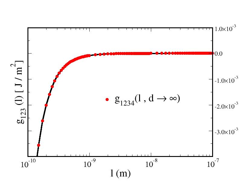
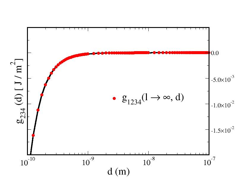
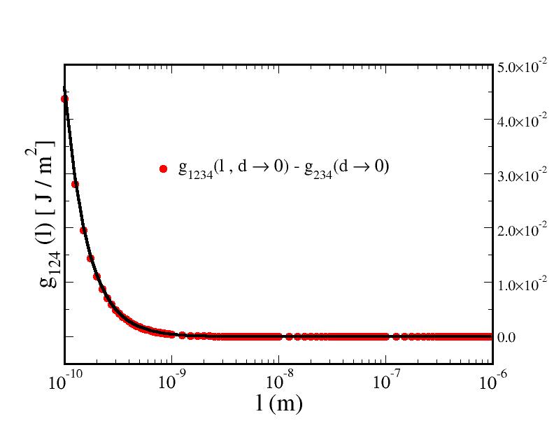
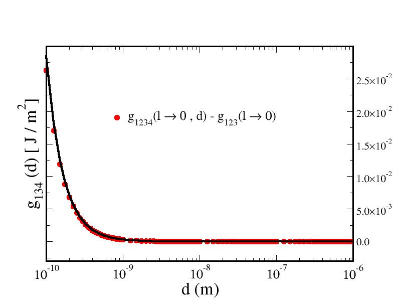
Figure 2: Limiting cases of $g_{1234}(l,d)$ at infinite and zero thicknesses. Top left exposes the case contained in Eq. 9, top right represents Eq. 10, bottom left displays the limit in Eq. 11, and bottom right the one in Eq. 12. Black lines correspond to exact calculations of the interface potentials indicated on the y axis, while the symbols are the corresponding prediction obtained from $g_{1234}(l,d)$ as indicated in the cited equations. The labels 1, 2, 3, 4 stand for AgI, ice, water and vapor, respectively. In practice for numerical purposes the large thickness limit is evaluated at $10^{-2}$ m, while the vanishing thickness limit is evaluated at $10^{-12}$ m. All surface energies are given in $J/m^{2}$.

V.2 Numerical checks

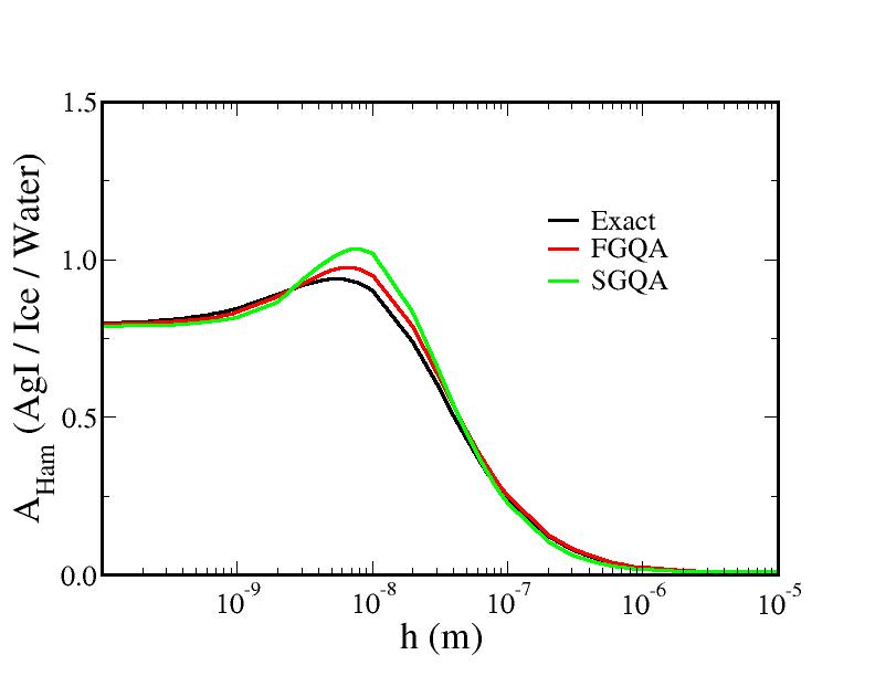
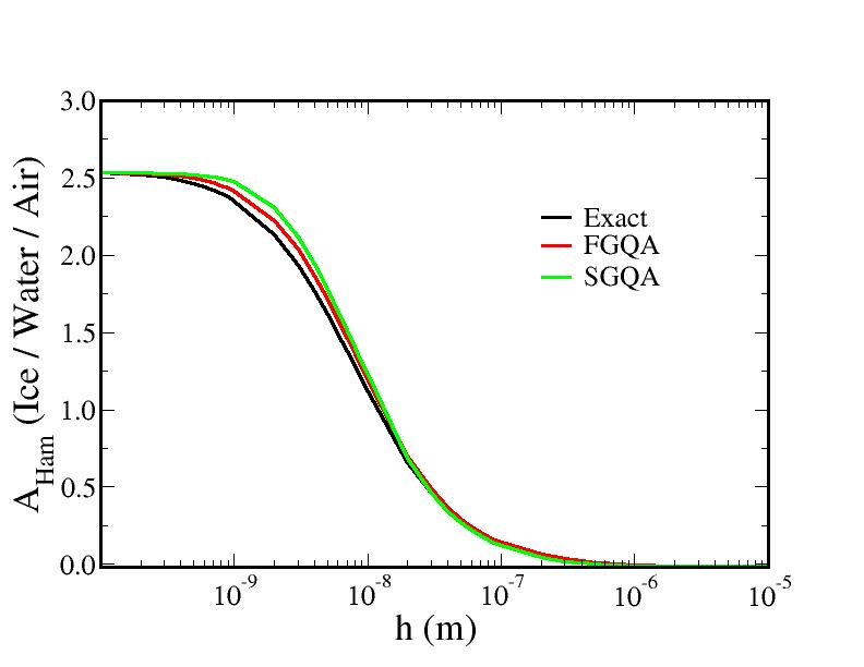
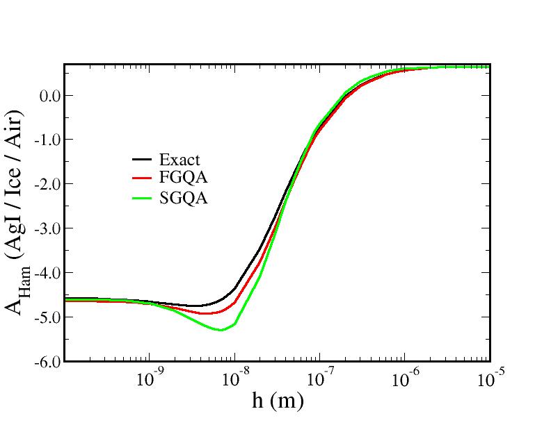
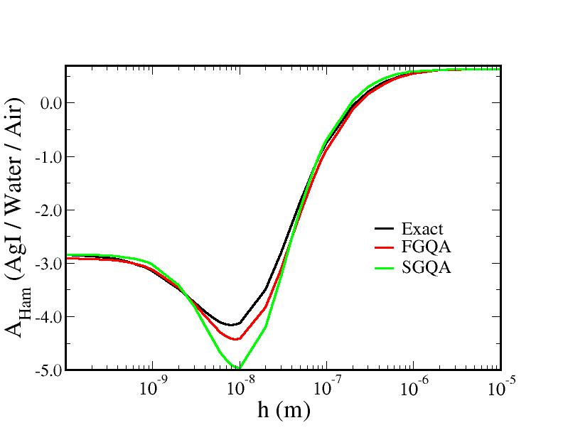
Figure 3: Comparison of exact Hamaker functions with analytical approximations. The $\nu_{\infty}$ parameter for the SGQA representation is indicated below in each corresponding case. Here we show all relevant combinations of three media formed from AgI, ice, water and vapor: AgI/Ice/Water (top left, $\nu_{\infty}=1.16\times 10^{8}\ m^{-1}$), Ice/Water/Air (top right, $\nu_{\infty}=4.10\times 10^{8}\ m^{-1}$), AgI/Ice/Air (bottom left, $\nu_{\infty}=1.01\times 10^{8}\ m^{-1}$) and AgI/Water/Air (bottom right, $\nu_{\infty}=1.11\times 10^{8}\ m^{-1}$). Results are given in units of $k_{B}T$.

Next we demonstrate the reliability of the First Gaussian Quadrature Approximation (FGQA) and the Second Gaussian Quadrature Approximation (SGQA) by comparing the outcomes for the three media Hamaker function (Eq. 1). The exact result is obtained using the general expression Eq.6, under the limiting conditions described in Eq.9-10, while the FGQA calculation is performed through Eq. 16 and Eq.15. The computation of the SGQA in Eq. 18 needs the knowledge of the $\nu_{\infty}$ parameter. We achieve this by requiring the approximate expression, Eq.18 to match the exact free energy in the limit of vanishing film thickness.

$$g_{123}^{SGQA}(h\to 0)=g_{123}^{exact}(h\to 0)$$ (28)

Essentially, this amounts to setting $\nu_{\infty}$ so as to match the exact Hamaker constant.
Figure 3 presents the three media Hamaker function of the systems AgI/Ice/Water, Ice/Water/Air, AgI/Ice/Air and AgI/Water/Air, and illustrates the accuracy of the analytic approximations that we have developed. The resulting Hamaker functions have been divided by $k_{B}T$ at this representation in order to make their values easier to handle, and offering also a ratio of their strength with respect to the thermal energy.
With $g_{AgI/Ice/Water}$ and $g_{Ice/Water/Air}$ we have the first two terms required to describe completely the free energy of the system (Eq. 13). The remaining contribution is given by $\Delta g_{1234}(l,d)$. We compare the exact result with the Second Gaussian Quadrature Approximation under the Similar Dielectric Function Approximation (SDF-SGQA) of Eq.24 in Fig.4. As before, the computation of SDF-SGQA requires explicit evaluation of the parameter $\nu_{\infty}$. This is achieved by requiring that the approximate result matches the exact value of $\Delta g_{1234}(l,d)$ in Eq. 20 in the limit $l=d$ and $(l+d)\to 0$.

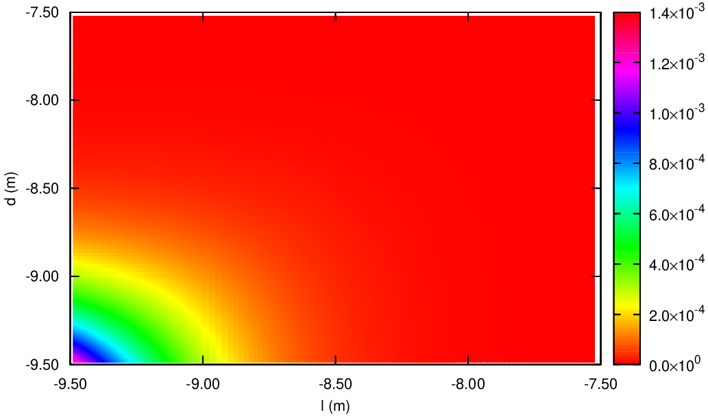
Figure 4: Correction $\Delta g_{1234}(l,d)$ obtained from the exact expression (left) and from the SDF-SGQA (right). The SFD-SGQA result is evaluated here using the parameter $\nu_{\infty}=1.06\times 10^{8}\ m^{-1}$. The correction supplies a repulsive contribution when both thicknesses (’l’ for ice and ’d’ for liquid water) are low, preventing the total $g_{1234}(l,d)$ to present an absolute minimum when both the liquid water layer and the ice layer disappear. Here the thicknesses are displayed in decimal logarithmic scale and surface energies are given in $J/m^{2}$.

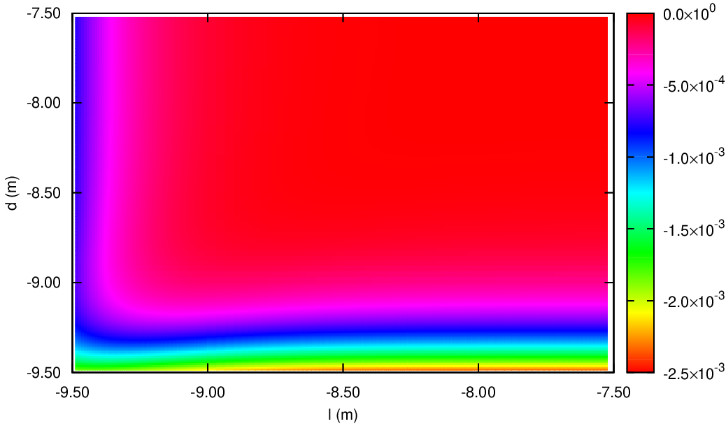
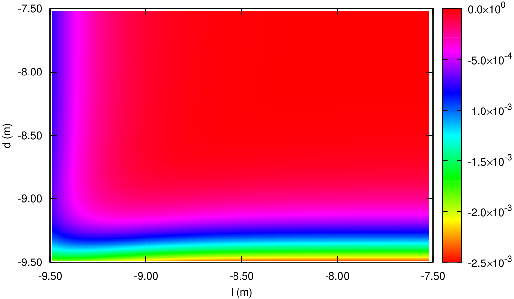
Figure 5: Comparison of the full interface potential from numerical results with theoretical calculations. Exact $g_{1234}(l,d)$ (left), obtained from the Eq. 6 with the dispersion relation of Eq. 7. FGQA of $g_{1234}(l,d)$ (right) under the SDF approximation. In both cases, the axes ’l’ and ’d’ are the thicknesses of the ice and the liquid water layers represented in decimal logarithmic scale, while surface free energies are given in $J/m^{2}$.

The numerical solution of the exact formula (Eq. 6) with the dispersion relation of Eq. 7 is presented in Fig. 5, left. The range is fixed from 0.3 nm to 30 nm, which is approximately the expected range of lengths of relevance of the Van der Waals forces, but the behavior is quite monotonous for wider thicknesses. This result is then taken as a reference to compare with energy curves emerging from the employment of the First Gaussian Quadrature under the Similar Dielectric Function approximation (Fig. 5, right), whose results arise from solving equations 15, 16 and 23. The outcome never exceeds a relative error of 3% with respect to the exact result. Since we have proved how good this approximation works, we can now take advantage of its drastically lower computation time to perform a more exhaustive calculation of $g_{1234}(l,d)$, using now a finer mesh that otherwise would require a huge amount of time to be completed.

The FGQA approximation has also the advantage of being quite easier to compute in terms of complexity of the algorithm. The computation of the SGQA is even faster, but requires the calculation of the $\nu_{\infty}$ parameter.

V.3 Van der Waals forces of Water and ice adsorbed on AgI

V.3.1 Three media systems

In this section, we discuss the implications of every three media - Hamaker function displayed in Fig. 3.

Recall that from Eq. 1, the $A_{Ham}(h)$ has opposite sign to $g_{123}(h)$. Thus the AgI/Ice/Water and Ice/Water/Air functions (top in Fig. 3) provide a negative surface free energy, with absolute minima at vanishing film thickness. This means that van der Waals forces do not favor the growth of ice at the AgI/water interface, and do not favor the growth of a premelting film of water at the ice/air interface either.

On the other hand, both the AgI/Ice/Air and AgI/Water/Air systems (Fig. 3, bottom) present negative values of the Hamaker function, which implies positive and monotonous decreasing surface free energies. Accordingly, van der Waals forces favor the growth of both ice and water thick films at the AgI/air interface.

In practice, the ultimate behavior of growing films on the AgI surface is dictated by a balance of short range structural forces and long range van der Waals forces. Since the ice/air interface is known to exhibit a significant amount of premelting slater19 , and van der Waals forces appear to inhibit growth of a liquid film, we conclude that the existence of premelting on ice is the result of short range structural forces, in agreement with recent findings from computer simulation limmer14 ; benet19 ; llombart20 .

V.3.2 AgI/Ice/Water/Air

Once again, recall that according to Eq. 13, the four media Van der Waals free energy, $g_{1234}(l,d)$, is given as the sum of two three-media contributions and $\Delta g_{1234}(l,d)$. The results for the four media surface free energy, displayed in the Fig. 5 (either left or right), illustrate how as ’l’ (the ice width) increases, the Van der Waals free energy in the Eq. 13 is completely governed by $g_{234}(d)$, and analogously, if ’d’ (water layer thickness) becomes very large, the system behaves as if the air was not there, and the whole dispersive interaction comes now by the hand of $g_{123}(l)$. When ’l’ and ’d’ are negligible, the $\Delta g_{1234}(l,d)$ term in Eq. 13 contributes with a positive energy, so that the total $g_{1234}(l,d)$ of the system does not have an absolute minimum at $l=d=0$.
Looking closely figure 5 at this scale, we appreciate how the lower set of minima appears for extremely low ’d’ ($d\rightarrow 0$, liquid water almost disappear) and for several - increasing values of ice width. Indeed, the Lifshitz theory extended to four media supports and confirms an intuitive result from the comparison between the Hamaker functions of three media systems in the previous section: the Van der Waals interactions favor the growth of either ice or water at the AgI/air interface only if the thickness of the other substance (water or ice) remains close to zero.

This is confirmed by noticing that $g_{1234}(l,d)<0$ at the bottom left corner of Fig.5. According to Eq.5 this implies that the surface tension $\gamma_{AgI/air}$ is smaller than the sum of $\gamma_{AgI/ice}$, $\gamma_{ice/water}$ and $\gamma_{water/air}$, implying that the adsorption of large ice and water films in between the AgI/air interface is unfavorable.

V.3.3 AgI/Water/Ice/Air

We have assumed all along that the nucleation occurs with the arrangement AgI/Ice/Water/Air. Nevertheless, this is not necessarily true, and it worth to check the behavior of the system AgI/Water/Ice/Air. For this purpose we solve numerically the exact Eq. 6 with the dispersion relation of Eq. 7, but this time with the following meaning of the indices: 1 = AgI, 2 = Liquid Water, 3 = Ice, 4 = Air. The result is presented in Fig. 6,

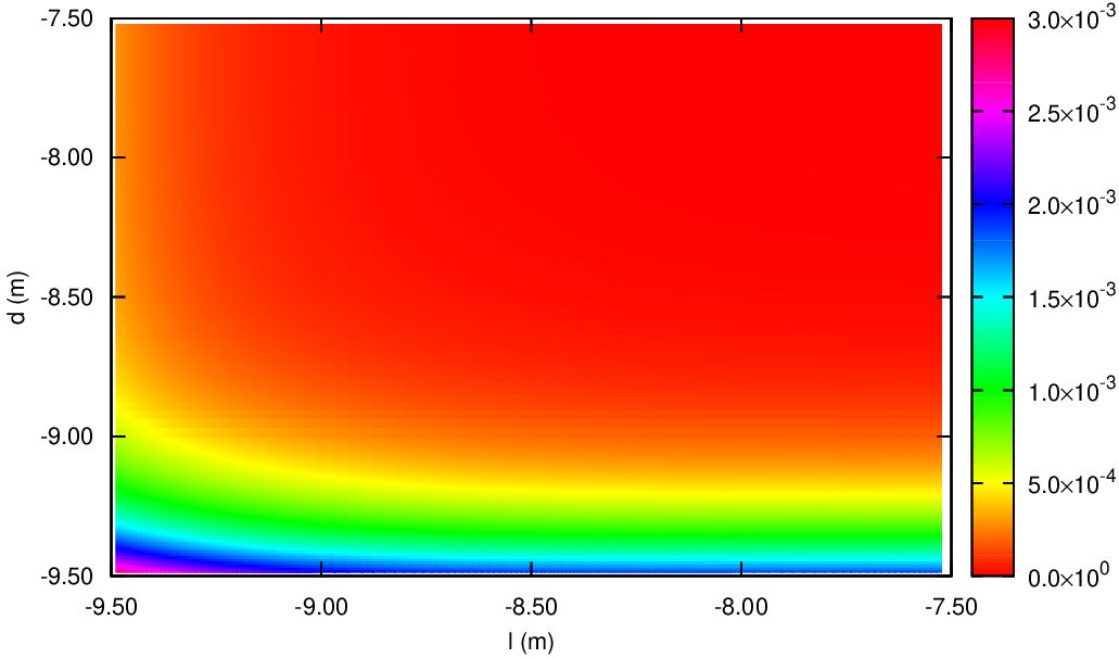
Figure 6: Surface free energy for $g_{1234}(l,d)$ and the layer order AgI/Water/Ice/Air. The axes ’l’ and ’d’ are now the thicknesses of the liquid water and the ice layers, in decimal logarithmic scale. Surface free energies in $J/m^{2}$.

The resulting interface potential is a positive (and therefore repulsive) energy, whose zeros (minima) are placed at large values of both thicknesses, meaning that the system will try to lower its energy by increasing the amount of both substances. Therefore, it appears that diverging layers of condensed water can grow on AgI if water is first adsorbed onto AgI and ice grows in between water and air. On the contrary, growth of ice in between AgI and water is not favored. The origin of this difference can be traced to the larger propensity of ice to grow in between water and air than that of water to form in between ice and air. This can be checked by looking at Fig. 6 along the axis of large water thickness, where it is seen that the free energy decreases by letting ice grow. This corresponds to the phenomenon of surface freezing, which here is seen to be favored by van der Waals forces, consistent with recent calculations fiedler20 .

V.3.4 Mechanism of ice nucleation

We will use this last part of the discussion to summarize some conclusions and considerations about the role of AgI as an ice nucleator.

Our results show that van der Waals forces promote the condensation of both ice and water on the AgI/air interface, a result which appears to be quite in agreement with the known nucleation efficiency of AgI marcolli16 . In fact, we find that the Hamaker constant of the AgI/ice/air system is larger (in absolute value) than that of AgI/water/air. This means that van der Waals forces actually promote the freezing of water vapor over the condensation of liquid water onto AgI. This expectation from the Hamaker constants is confirmed by inspection of Fig.5, which shows that indeed, the free energies along the $d\to 0$ axis of vanishing water thickness are more negative than those found along the $l\to 0$ axis of vanishing ice thickness.

On the contrary, it is found that van der Waals forces do not promote ice growth at the AgI/water surface. This can be read off from Fig.5, by looking at the free energy along the $d\to\infty$ axis, or merely, by inspection of the Hamaker function of the AgI/ice/water system, Fig.3.

From these observations, we can conclude that van der Waals forces actually favor a deposition mode of ice nucleation from the vapor phase. Of course, this is quite at odds with experimental findings, which show that AgI can nucleate ice both from vapor or water at a similar undercooling of about 4 °C pruppacher10 .

The reason for this apparent discrepancy is that the ultimate behavior of the system is dictated by a balance of both structural and van der Waals forces. Since an undercooling of at least 4 °C is required for ice to grow from supercooled water vapor, there must be short range structural forces which oppose mildly to ice growth. Otherwise, in the absence of short range forces, van der Waals forces would favor nucleation of ice from the vapor without any undercooling. This is very much consistent with computer simulations by Shevkunov, which indicate that a one monolayer thick ice film can form at ice vapor saturation, but further growth is mildly activated shevkunov05 .

On the contrary, van der Waals forces do not promote ice growth for AgI immersed in water, but simulations consistently show that Ag⁺ exposed surfaces readily nucleate ice at mild supercooling fraux14 ; zielke15 ; glatz16 . This means that short range structural forces do favor ice growth at the AgI/water surface, and a small activation is required because of the unfavorable van der Waals interactions.

Interestingly, it has been suggested that AgI is actually most efficient in the contact mode, whereby ice nucleation is promoted for AgI particles in contact with condensed water droplets marcolli16 . An explanation for this effect can be provided by assuming that nucleation actually occurs at the three phase contact line formed between AgI, water and air djikaev08 , but this requires a favorable line tension. Our results lend support to such favorable phenomenon. Indeed, we find that van der Waals forces promote growth of a thin ice layer on AgI in contact with water vapor. Such growth is ultimately very slow, because of the low vapor pressure of ice. However, if such thin ice layer is formed at the contact line of an AgI particle with the air/water interface, a large reservoir of undercooled bulk water would be made available for the thin ice layer to continue growing at the water/air interface, where, as we have seen, van der Waals forces promote surface freezing.

VI Conclusions

In this study we work out the exact Lifshitz theory of van der Waals forces for a substrate in the neighborhood of three phase coexistence, where two adsorbed layers of variable thickness can form on the substrate. The adsorption equilibrium is set by an underlying interface potential, as in the Frumkin-Derjaguin theory of adsorption churaev95 , but depends on the thickness of the two adsorbed layers. Our approach goes well beyond a Hamaker theory of pairwise additive forces that is conventionally employed in colloidal science hough80 ; bergstrom97 ; loskill12 ; simavilla18 , and extends previous results for a single adsorption layer on substrates with coatings of fixed thickness ninham70c ; podgornik03 ; parsegian05 .

Accurate analytical approximations are provided which improve conventional treatments of non-retarded van der Waals forces israelachvili11 and apply also to the regime of retarded interactions. This extends the validity of the calculations from film thicknesses barely decades of nanometers to arbitrary large values. Unlike the Gregory equation advocated by Israelachvili israelachvili11 , this is achieved without any ad-hoc parameter gregory81 . By this token, we find one can now accurately evaluate the free energy in the Hamaker and Casimir regimes with the same data that is required to estimate Hamaker constants hough80 ; bergstrom97 ; butt10 ; israelachvili11 . The proper account of retardation does not only provide better accuracy. It is a major qualitative improvement, as the crossover from non-retarded to retarded interactions is often accompanied by a sign reversal of the van der Waals forces.

Our results are applied to the study of water vapor adsorption on AgI, where both layers of ice and water can form close to the triple point. Previous studies on the ice nucleation efficiency of AgI have provided insight into the short range interactions of either undercooled water or vapor with the AgI surface shevkunov05 ; fraux14 ; zielke15 ; glatz16 . However, in the atmosphere both ice and water compete simultaneously for the vapor phase and it is very difficult to assess the relative stability of thick water and ice films from simulation. Our results indicate that van der Waals forces stabilize the growth of ice films at the AgI/air interface, but on the contrary, inhibit the growth of ice in the immersion mode. Importantly, van der Waals forces also promote growth of thick ice films at the air/water interface. This explains the intriguing observation of sub-surface nucleation in experiments and computer simulations durant05 ; haji17 , but also helps understand how the water/AgI/air contact line could promote ice nucleation djikaev08 . The AgI/vapor surface provides the site for stabilized ice layers that serve as embryos for the growth of a stable ice film at the water/vapor interface, thus lending support to contact mode freezing of AgI particles found in experiments marcolli16 .

Our results provide a general framework to gauge the role of van der Waals forces in the colloidal sciences, where multicomponent solutions display multiphase coexistence ubiquitously, and provide a solid background to assess how long range forces condition the ice nucleation efficiency of atmospheric aerosols.

Authors Contributions

Juan Luengo-Márquez: Methodology, Formal analysis, Visualization, Software, Investigation, Writing-Original Draft; Luis G. MacDowell: Validation, Conceptualization, Methodology, Writing-Review and Editing.

Declaration of Competing Interests

There are no interests to declare.

Funding

This work was supported by the Spanish Agencia Estatal de Investigación under Grant No. FIS2017-89361-C3-2-P.

Data Statement

The data used in this work is available upon request to the corresponding author.

References

Supplementary Material
Lifshitz theory of wetting films at three phase coexistence: The case of ice nucleation on Silver Iodide (AgI)

Juan Luengo-Márquez and Luis G. MacDowell

1. Derivation of the dispersion relation of the exact Lifshitz formula

The dispersion relation of the system is an expression that all standing electromagnetic waves across the system must hold. These waves have an electric, $\vec{E}(t)$, and magnetic, $\vec{H}(t)$, field function of time, $t$, with the form

$$\vec{E}(t)=Re\left(\sum_{\omega}\vec{E}_{\omega}e^{-i\omega t}\right)$$ (29)

$$\vec{H}(t)=Re\left(\sum_{\omega}\vec{H}_{\omega}e^{-i\omega t}\right)$$ (30)

Being $i$ the imaginary unit, $\omega$ the frequency, and $\vec{E}_{\omega}$, $\vec{H}_{\omega}$ the amplitudes of every field at that frequency. Each must respect a certain wave equation

$$\nabla^{2}\vec{E}=\frac{\epsilon\mu}{c^{2}}\frac{\partial^{2}{\vec{E}}}{\partial{t}^{2}}$$ (31)

$$\nabla^{2}\vec{H}=\frac{\epsilon\mu}{c^{2}}\frac{\partial^{2}{\vec{H}}}{\partial{t}^{2}}$$ (32)

With $\epsilon$ and $\mu$ the dielectric and magnetic permeability and $c$ the velocity of light. We can turn Eq. 31 and 32 into differential equations of the components of the position solving the partial derivative with time from Eq. 29 and 30, respectively. In our system, the vectors $\vec{E}$ and $\vec{H}$ have periodic x, y components with the general form $f(z)e^{i(ux+vy)}$. Then solve the derivatives in the resulting differential equation to get the general $f^{\prime\prime}(z)=\rho_{k}^{2}f(z)$, with

$$\rho_{k}^{2}=u^{2}+v^{2}-\frac{\epsilon_{k}\mu_{k}\omega^{2}}{c^{2}}$$ (33)

Where we define later $\rho=u^{2}+v^{2}$. The general solution yields $f^{k}_{\alpha}(z)=A^{k}_{\alpha}e^{\rho_{k}z}+B^{k}_{\alpha}e^{-\rho_{k}z}$, with $\alpha=x,y,z$ for every substance $k$ at the system. Here we name the layers as 1/2/3/4. Finally, we impose $\nabla\cdot\vec{E}=0$ and $\nabla\cdot\vec{H}=0$ to reach that

$$A^{k}_{z}=-\frac{i}{\rho}(uA^{k}_{x}+vA^{k}_{y})$$ (34)

$$B^{k}_{z}=\frac{i}{\rho}(uB^{k}_{x}+vA^{k}_{y})$$ (35)

Which is true separately at every substance $k\ =$ ’1’, ’2’, ’3’, ’4’. Next let us apply the boundary conditions at every interface, setting the $z$ axis perpendicular to the interfaces and the $z=0$ point at the interface 1/2. Now the thickness of ’2’ will be ’l’ and that of the substance ’3’ will be ’d’.
$\bullet$ $z=0$, interface 1/2. Here $B^{1}_{x,y,z}$ must be zero so that $f^{1}$ does not go to infinite when z tends to $-\infty$. Then we impose the conditions $E^{1}_{x}=E^{2}_{x}$ and $E^{1}_{y}=E^{2}_{y}$, sum the resulting equations and use Eq. 34 and 35 to get

$$-\rho_{1}A^{1}_{z}+\rho_{2}A^{2}_{z}-\rho_{2}B^{2}_{z}=0$$ (36)

On the other hand, it must also be true that $\epsilon_{1}E^{1}_{z}=\epsilon_{2}E^{2}_{z}$, that is

$$\epsilon_{1}A^{1}_{z}=\epsilon_{2}A^{2}_{z}+\epsilon_{2}B^{2}_{z}$$ (37)

$\bullet$ $z=l$, interface 2/3. Here we apply basically the same procedure. Notice that now the exponentials do not vanish, so we reach from $E^{2}_{x}=E^{3}_{x}$ and $E^{2}_{y}=E^{3}_{y}$

$$-\rho_{2}A^{2}_{z}e^{\rho_{2}l}+\rho_{2}B^{2}_{z}e^{-\rho_{2}l}+\rho_{3}A^{3}_{z}e^{\rho_{3}l}-\rho_{3}B^{3}_{z}e^{-\rho_{3}l}=0$$ (38)

And from the condition $\epsilon_{2}E^{2}_{z}=\epsilon_{3}E^{3}_{z}$

$$\epsilon_{2}A^{2}_{z}e^{\rho_{2}l}+\epsilon_{2}B^{2}_{z}e^{-\rho_{2}l}=\epsilon_{3}A^{3}_{z}e^{\rho_{3}l}+\epsilon_{3}B^{3}_{z}e^{-\rho_{3}l}$$ (39)

$\bullet$ $z=l+d$, interface 3/4. Here $A^{4}_{x,y,z}$ must be zero so that $f^{4}$ does not go to infinite as z tends to $\infty$. From $E^{3}_{x}=E^{4}_{x}$ and $E^{3}_{y}=E^{4}_{y}$ now we have

$$-\rho_{3}A^{3}_{z}e^{\rho_{3}(l+d)}+\rho_{3}B^{3}_{z}e^{-\rho_{3}(l+d)}-\rho_{4}B^{4}_{z}e^{-\rho_{4}(l+d)}=0$$ (40)

And finally, from $\epsilon_{3}E^{3}_{z}=\epsilon_{4}E^{4}_{z}$ we get

$$\epsilon_{3}A^{3}_{z}e^{\rho_{3}(l+d)}+\epsilon_{3}B^{3}_{z}e^{-\rho_{3}(l+d)}=\epsilon_{4}B^{4}_{z}e^{-\rho_{4}(l+d)}$$ (41)

So far we have used the boundaries for the electric fields. Solving the system of equations formed by Eq. 36, 37, 38, 39, 40 and 41 for the six variables $\{A_{i}\}$, $\{B_{i}\}$, leads to what equalized to zero is the dispersion relation of the system $D_{M}=0$. For that we just arrange those equations in the determinant

$\left|\begin{array}[]{cccccc}-\rho_{1}&\rho_{2}&-\rho_{2}&0&0&0\\ \epsilon_{1}&-\epsilon_{2}&-\epsilon_{2}&0&0&0\\ 0&-\rho_{2}e^{\rho_{2}l}&\rho_{2}e^{-\rho_{2}l}&\rho_{3}e^{\rho_{3}l}&-\rho_{3}e^{-\rho_{3}l}&0\\ 0&\epsilon_{2}e^{\rho_{2}l}&\epsilon_{2}e^{-\rho_{2}l}&-\epsilon_{3}e^{\rho_{3}l}&-\epsilon_{3}e^{-\rho_{3}l}&0\\ 0&0&0&-\rho_{3}e^{\rho_{3}(l+d)}&\rho_{3}e^{-\rho_{3}(l+d)}&-\rho_{4}e^{-\rho_{4}(l+d)}\\ 0&0&0&\epsilon_{3}e^{\rho_{3}(l+d)}&\epsilon_{3}e^{-\rho_{3}(l+d)}&-\epsilon_{4}e^{-\rho_{4}(l+d)}\end{array}\right|=D_{M}$

Solving for the determinant explicitly gives a sum of 32 terms which is not particularly insightful. However, one notices that products of two matrix elements of the form $d_{ij}d_{kl}$ have common factors with terms $d_{il}d_{kj}$, or alternatively, terms of the form $\rho_{i}\epsilon_{j}$ share common factors with $\rho_{j}\epsilon_{i}$. Therefore, we organize the 32 terms as:

$$\begin{array}[]{c}D_{M}=\\ (\rho_{1}\epsilon_{2}-\rho_{2}\epsilon_{1})\left[(\rho_{4}\epsilon_{3}-\rho_{3}\epsilon_{4})(\rho_{2}\epsilon_{3}+\rho_{3}\epsilon_{2})\alpha^{-1}\beta\gamma^{-1}+(\rho_{4}\epsilon_{3}+\rho_{3}\epsilon_{4})(\rho_{3}\epsilon_{2}-\rho_{2}\epsilon_{3})\alpha^{-1}\beta^{-1}\gamma\right]\delta^{-1}\\ +\\ (\rho_{2}\epsilon_{1}+\rho_{1}\epsilon_{2})\left[(\rho_{2}\epsilon_{3}-\rho_{3}\epsilon_{2})(\rho_{3}\epsilon_{4}-\rho_{4}\epsilon_{3})\alpha\beta\gamma^{-1}-(\rho_{3}\epsilon_{2}+\rho_{2}\epsilon_{3})(\rho_{4}\epsilon_{3}+\rho_{3}\epsilon_{4})\alpha\beta^{-1}\gamma\right]\delta^{-1}\end{array}$$ (42)

where we have introduced the symbols $\alpha=e^{\rho_{2}l}$, $\beta=e^{\rho_{3}l}$, $\gamma=e^{\rho_{3}(l+d)}$ and $\delta=e^{\rho_{4}(l+d)}$, for short.

Notice now that the determinant is a product of elements $(\rho_{i}\epsilon_{j}+\rho_{j}\epsilon_{i})$, which correspond to denominators of the function $\Delta_{ij}^{M}$ in the main text (see also below, Eq.44); and elements $(\rho_{i}\epsilon_{j}-\rho_{j}\epsilon_{i})$ which correspond to numerators of $\Delta_{ij}^{M}$. Since, from the dispersion relation, this determinant must vanish, we can now multiply and divide by constants without changing the result. Therefore, we divide by factors of the form $(\rho_{i}\epsilon_{j}+\rho_{j}\epsilon_{i})$, and further divide by $\alpha\beta^{-1}\gamma\delta^{-1}$ to get:

$$D_{M}=1-\Delta^{M}_{12}\Delta^{M}_{32}e^{-2\rho_{2}l}-\Delta^{M}_{23}\Delta^{M}_{43}e^{-2\rho_{3}d}-\Delta^{M}_{12}\Delta^{M}_{43}e^{-2\rho_{2}l}e^{-2\rho_{3}d}$$ (43)

$$\Delta^{M}_{ij}=\frac{\rho_{j}\epsilon_{i}-\rho_{i}\epsilon_{j}}{\rho_{j}\epsilon_{i}+\rho_{i}\epsilon_{j}}$$ (44)

which is the sought result. Notice that here $l$ and $d$ stand on the same footing.

The result for a system of one single medium between two plates, with one plate coated by a layer of fixed thickness, $d$, can be obtained from this expression readily. In that situation the physical requirement is that $D_{M}\to 1$, as $l\to\infty$ at fixed $d$. From Eq.43, we find instead:

$$\lim_{l\to\infty}D_{M}=1-\Delta_{23}^{M}\Delta_{43}^{M}e^{-2\rho_{3}d}$$ (45)

Therefore, a new function consistent with the mentioned physical requirement can be obtained simply dividing $D_{M}$ by $\lim_{l\to\infty}D_{M}$. This yields:

$$D^{\prime}_{M}=1-\frac{\Delta_{12}^{M}\Delta_{32}^{M}+\Delta_{12}^{M}\Delta_{43}^{M}e^{-2\rho_{3}d}}{1-\Delta_{23}^{M}\Delta_{43}^{M}e^{-2\rho_{3}d}}e^{-2\rho_{2}l}$$ (46)

which is the well known relation used for systems with one coated layer of fixed size. Because of the choice of normalization condition, the variables $l$ and $d$ no longer stand on the same footing.

The calculation of $D_{E}$ arises from a similar analysis of the boundaries for the magnetic fields, and takes the same form as Eq.(43), with $\Delta_{ij}^{M}$ merely replaced by $\Delta_{ij}^{E}$,

$$\Delta^{E}_{ij}=\frac{\rho_{j}-\rho_{i}}{\rho_{j}+\rho_{i}}$$ (47)

With $D_{E}$ and $D_{M}$ at hand, we readily obtain $D=D_{M}\cdot D_{E}$, which can be plugged into the general expression for the interface potential, Eq.(6) of the main text. Alternatively, we can transform $D_{E}$ to obtain $D^{\prime}_{E}$ in the same way as we obtained $D^{\prime}_{M}$, which yields $D^{\prime}=D^{\prime}_{E}\cdot D^{\prime}_{M}$.

The significance of this transformation may be understood by noticing that we have defined in practice:

$$D^{\prime}_{1234}(l;d)=D_{1234}(l,d)\left/D_{1234}(l\to\infty,d)\right.$$ (48)

where the prime next to D and the arguments $(l;d)$ in the left hand side indicate that the thickness ’d’ is now meant as a fixed parameter, not a variable.

Plugging this result into Eq.(6) of the main text, we readily find:

$$g^{\prime}_{1234}(l;d)=\frac{k_{B}T}{2\pi}{\sum_{n=0}^{\infty}}^{\prime}\int_{0}^{\infty}\rho\hskip 2.84544ptd\rho\ln\left(\frac{D_{1234}(l,d)}{D_{1234}(l\to\infty,d)}\right)$$ (49)

By splitting the logarithm into two different additive contributions, we readily find:

$$g^{\prime}_{1234}(l;d)=g_{1234}(l,d)-g_{1234}(l\to\infty,d)$$ (50)

Whence, the known results for the interface potential of a system with layer ’2’ of variable thickness $l$ and a coating of fixed thickness $d$ obtained previously in Ref.26–28. differs from the full two variable interface potential merely by a normalization constant, which sets the requirement that $g^{\prime}_{1234}(l;d)$ vanishes in the limit that $l\to\infty$. Alternatively, noticing that in fact $g_{1234}(l\to\infty,d)$ corresponds to the interface potential for a three media system of layer ’3’ sandwiched between semi-infinite bodies ’2’ and ’4’ (c.f. Eq.(10) of main text), the above result may be readily written as:

$$g^{\prime}_{1234}(l;d)=g_{1234}(l,d)-g_{234}(d)$$ (51)

Particularly, in the limit that $d$ vanishes altogether, $g^{\prime}_{1234}(l;d\to 0)$ becomes $g_{124}(l)$, so we find:

$$g_{124}(l)=g_{1234}(l,d\to 0)-g_{234}(d\to 0)$$ (52)

which is Eq.(11) of the main text. A similar analysis holds for the case $l\to 0$, which corresponds to Eq.(12) of the main text.

2. Change of variable to ’x’

Our purpose here is to develop explicitly the route from the three media exact surface free energy to the equation over which the First Gaussian Quadrature Approximation is performed, Eq.14 of the main text. Then we start from the generalized form of the three media surface potential

$$g_{123}(h)=\frac{k_{B}T}{2\pi}{\sum^{\infty}_{n=0}}^{\prime}\int_{0}^{\infty}\rho\hskip 1.42271ptd\rho\ln(D^{E}_{123}D^{M}_{123})$$ (53)

Where ’$h$’ stands for the thickness of the layer ’$2$’ and the prime next to the sum indicates that the term $n=0$ has an extra factor $1/2$. The dispersion relation is that of the three layered media geometry, as dictated by $D^{E,M}_{123}=1-\Delta^{E,M}_{12}\Delta^{E,M}_{32}e^{-2\rho_{2}h}$. Next we assume that the term after the 1 at $D^{E,M}_{123}$ is small, and we expand the logarithm as $ln(1-x)\approx=-x$. At the same time, let us change the variable to $\rho_{2}^{2}=\rho^{2}+\frac{\epsilon_{2}\xi_{n}^{2}}{c^{2}}$. We perform this transformation simply through $\rho_{2}d\rho_{2}=\rho d\rho$, and the lower limit of the integral now is $\rho_{2}(\rho=0)=\sqrt{\frac{\epsilon_{2}\xi_{n}^{2}}{c^{2}}}$

$$g_{123}(h)=-\frac{k_{B}T}{2\pi}{\sum^{\infty}_{n=0}}^{\prime}\int_{\sqrt{\frac{\epsilon_{2}\xi_{n}^{2}}{c^{2}}}}^{\infty}\rho_{2}\hskip 1.42271ptd\rho_{2}(\Delta^{M}_{12}\Delta^{M}_{32}+\Delta^{E}_{12}\Delta^{E}_{32})e^{-2\rho_{2}h}$$ (54)

With $\Delta^{M}_{ij}$ and $\Delta^{E}_{ij}$ as defined in Eq. 44 and Eq.47.

In the last step we perform a second change of variables to $x=2\rho_{2}h$, so that $x\hskip 1.42271ptdx=4h^{2}\rho_{2}\hskip 1.42271ptd\rho_{2}$. Moreover, the lower limit is transformed again to $2h\sqrt{\frac{\epsilon_{2}\xi_{n}^{2}}{c^{2}}}$, which we define as $r_{n}$

$$g_{123}(h)=-\frac{k_{B}T}{8\pi h^{2}}{\sum^{\infty}_{n=0}}^{\prime}\int_{r_{n}}^{\infty}x\hskip 1.42271ptdx(\Delta^{M}_{12}\Delta^{M}_{32}+\Delta^{E}_{12}\Delta^{E}_{32})e^{-x}$$ (55)

Both $\Delta^{M}_{ij}$ and $\Delta^{E}_{ij}$ may be expressed in terms of $x_{i}=\sqrt{x^{2}+(\epsilon_{i}-\epsilon_{2})(2h\xi_{n}/c)^{2}}$ instead of $\rho_{i}$, through the straightforward substitution $x_{i}=2\rho_{i}h$. The Eq. 55 corresponds to the stage immediately before the FGQA at the main part of the work, and is the result to which we wanted to arrive here.

3. Gaussian Quadrature

The Gaussian quadrature is an integration method where the integrand is separated between a well shaped function, $f(x)$, and a weight function, $w(x)$. The generalized N points Gaussian quadrature reads

$$\int_{a}^{b}f(x)w(x)dx=\sum_{i=1}^{N}f(x_{i})m_{i}$$ (56)

With $f(x)$ evaluated at the nodes $x_{i}$ (also called quadrature points). The knowledge of the sets of $\{x_{i}\}$ and $\{m_{i}\}$ requires the capability of solving from the $j=0$ up to the $2N-1$ integral of the kind

$$I_{j}=\int_{a}^{b}x^{j}w(x)dx=\sum_{i=1}^{N}x_{i}^{j}m_{i}$$ (57)

That leads to a system of 2N equations whose solution provides the quadrature points and all $\{m_{i}\}$. In this work we have used the one point Gaussian quadrature (N=1), so the integrals that we have to solve are

$$I_{0}=\int_{a}^{b}w(x)dx$$ (58)

$$I_{1}=\int_{a}^{b}x\hskip 1.42271ptw(x)dx$$ (59)

Thus we have $m_{1}=I_{0}$, and $x_{1}=I_{1}/I_{0}$.

4. One point Gaussian quadrature applied to the FGQA

We wish to specify here the quadrature performed over

$$g^{\xi_{n}>0}(h)=-\frac{k_{B}T}{8\pi h^{2}}\sum^{\infty}_{n=1}\int_{r_{n}}^{\infty}x\hskip 1.42271ptdxR(n,x)e^{-x}$$ (60)

which is written here in generalized form so that it applies both for $g_{123}(h)$ and $\Delta g_{1234}(l,d)$. In the last case just consider that $h=(l+d)$, and employ $R^{e}(n,x)$ instead of $R(n,x)$. We state then $f(x)=R(n,x)$, and $w(x)=xe^{-x}$. Using this weight in Eq.58-59 provides straightforward integrals of the form

$$I_{0}=\int_{r_{n}}^{\infty}xe^{-x}dx=e^{-r_{n}}(1+r_{n})$$ (61)

$$I_{1}=\int_{r_{n}}^{\infty}x^{2}e^{-x}dx=e^{-r_{n}}(2+2r_{n}+r_{n}^{2})$$ (62)

5. Euler - MacLaurin formula

The Euler-MacLaurin formula allows the transformation of a summation into an integral through an approximation, and reads

$$\sum_{n=a}^{b}f(n)=\int_{a}^{b}f(n)dn+\frac{1}{2}(f(a)+f(b))+\sum^{\infty}_{k=1}\frac{B_{2k}}{2k!}(f^{(2k-1)}(b)-f^{(2k-1)}(a))$$ (63)

$B_{i}$ being the Bernoulli coefficients and $f^{(m)}$ the m-th derivative of $f$. From now on we will apply it up to the first corrective order, $k=1$.
We start again from the generalization presented in the previous section. We have after the FGQA the expression

$$g^{\xi_{n}>0}(h)=-\frac{k_{B}T}{8\pi h^{2}}\sum^{\infty}_{n=1}R(n,x_{1})(1+r_{n})e^{-r_{n}}$$ (64)

And now we evaluate the corrective term of the Eq. 63, considering that $R(n,x_{1})$ is essentially constant with $n$ compared to the exponential dependence. This is also true for the $\Delta g_{1234}(l,d)$ particularization, since even if the exponential in $R^{e}(n,x_{1})$ contains a $n^{2}$ factor, the value of $\Delta\epsilon$ is extremely close to zero for large $n$, and the value of $(d^{2}-l^{2})$ is quite small as well. These features make that exponential factor very close to one. The corrective term of the Euler-MacLaurin formula is then

$$\Delta g^{\xi_{n}>0}=-\frac{k_{B}T}{8\pi h^{2}}\left[\frac{1}{2}R(1,x_{1})(1+r_{T})e^{-r_{T}}+\frac{1}{12}R(1,x_{1})r_{T}^{2}e^{-r_{T}}\right]$$ (65)

Where $r_{T}=r_{n=1}$. For most cases of interest, where $\nu_{T}h\ll 1$, this term is negligible and adds a correction of order $\nu_{T}/\nu_{\infty}$ to the Hamaker constant. In the regime where $\nu_{T}h\approx 1$, it exhibits the same order of magnitude as the leading order term, and does therefore not upset the scaling. However, in that range the finite frequency contribution becomes negligible compared to the $n=0$ term, so it is save to neglect it altogether. Accordingly, we neglect the corrections here for the sake of simplicity and use the approximation:

$$g^{\xi_{n}>0}(h)=-\frac{k_{B}T}{8\pi h^{2}}\int^{\infty}_{1}R(n,x_{1})(1+r_{n})e^{-r_{n}}dn$$ (66)

The following step is to change the variable to $\nu=(4\pi k_{B}T\epsilon^{1/2}_{2}n)/(c\hbar)$. Realize that $\epsilon_{2}$ is also a function of n, so we change the variable through

$$d\nu=\frac{4\pi k_{B}T}{c\hbar}\epsilon^{1/2}_{2}dn\left[1+\frac{1}{2}\frac{d\ln\epsilon_{2}}{d\ln\xi_{n}}\right]$$ (67)

The term inside the brackets is defined as $j_{2}$, and its value is approximately 1. If the last transformations are to be performed at $\Delta g_{1234}(l,d)$, we employ $\epsilon_{1/2}$ instead of $\epsilon_{2}$, and correspondingly, we define $j_{1/2}$ instead of $j_{2}$. Once the variable is changed we achieve

$$g^{\xi_{n}>0}(h)=-\frac{c\hbar}{32\pi^{2}h^{2}}\int^{\infty}_{\nu_{T}}\widetilde{R}(\nu,x_{1})(1+h\nu)e^{-h\nu}d\nu$$ (68)

Where $\widetilde{R}(\nu,x_{1})=\epsilon_{2}^{-1/2}j_{2}^{-1}R(\nu,x_{1})$.

6. One point Gaussian quadrature applied to the SGQA

Beginning at the Eq. 68, we introduce the auxiliary exponential function $e^{-\nu/\nu_{\infty}}$, with the parameter $\nu_{\infty}$ chosen to mimic the scale at which the algebraic decay of $\widetilde{R}(\nu,x_{1})$ becomes significant

$$g^{\xi_{n}>0}(h)=-\frac{c\hbar}{32\pi^{2}h^{2}}\int^{\infty}_{\nu_{T}}\widetilde{R}(\nu,x_{1})e^{\nu/\nu_{\infty}}\left[e^{-\nu/\nu_{\infty}}(1+h\nu)e^{-h\nu}\right]d\nu$$ (69)

And next we perform the one point Gaussian quadrature approximation with $f(\nu)=\widetilde{R}(\nu,x_{1})e^{\nu/\nu_{\infty}}$, and $w(\nu)=e^{-\nu/\nu_{\infty}}(1+h\nu)e^{-h\nu}$. We solve then $I_{0}$ and $I_{1}$ by parts

$$I_{0}=\int_{\nu_{T}}^{\infty}e^{-\nu/\nu_{\infty}}(1+h\nu)e^{-h\nu}d\nu$$ (70)

$$I_{0}=\nu_{\infty}\frac{(\nu_{T}h+1)(\nu_{\infty}h+1)+\nu_{\infty}h}{(\nu_{\infty}h+1)^{2}}e^{-\nu_{T}h-\frac{\nu_{T}}{\nu_{\infty}}}$$ (71)

$$I_{1}=\int_{\nu_{T}}^{\infty}\nu e^{-\nu/\nu_{\infty}}(1+h\nu)e^{-h\nu}d\nu$$ (72)

$$I_{1}=\nu_{\infty}\frac{(\nu_{T}h+1)(\nu_{\infty}h+1)^{2}\nu_{T}+(2\nu_{T}h+1)(\nu_{\infty}h+1)\nu_{\infty}+2\nu_{\infty}^{2}h}{(\nu_{\infty}h+1)^{3}}e^{-\nu_{T}h-\frac{\nu_{T}}{\nu_{\infty}}}$$ (73)

7. Similar Dielectric Function approximation

In this section we intend to clarify the steps to follow throughout the development of the Similar Dielectric Function approximation. Starting from the correction term of the four media surface free energy

$$\Delta g_{1234}(l,d)=-\frac{k_{B}T}{2\pi}{\sum_{n=0}^{\infty}}^{\prime}\int_{0}^{\infty}\rho\ d\rho\ R_{1234}(n,\rho)\ e^{-2(\rho_{2}l+\rho_{3}d)}$$ (74)

We first notice from the definition of $\rho_{i}$ that one can write

$$\rho_{2}^{2}=\rho_{1/2}^{2}-\frac{1}{2}\frac{\Delta\epsilon}{c^{2}}\xi_{n}^{2}$$ (75)

$$\rho_{3}^{2}=\rho_{1/2}^{2}+\frac{1}{2}\frac{\Delta\epsilon}{c^{2}}\xi_{n}^{2}$$ (76)

Where we have introduced $\Delta\epsilon=\epsilon_{3}-\epsilon_{2}$, and $\rho_{1/2}^{2}=\rho^{2}+\frac{1}{2}\frac{(\epsilon_{3}+\epsilon_{2})}{c^{2}}\xi_{n}^{2}$. Then we assume small $\Delta\epsilon$ and apply Taylor to get

$$\rho_{2}\approx\rho_{1/2}-\frac{1}{4}\frac{\xi_{n}^{2}\Delta\epsilon}{c^{2}\rho_{1/2}}$$ (77)

$$\rho_{3}\approx\rho_{1/2}+\frac{1}{4}\frac{\xi_{n}^{2}\Delta\epsilon}{c^{2}\rho_{1/2}}$$ (78)

Using these results, the exponential function in Eq.74 can be now factored into two simpler exponentials:

$$e^{-2(\rho_{2}l+\rho_{3}d)}\approx e^{-2\rho_{1/2}(l+d)}e^{-\frac{1}{2}\frac{\xi_{n}^{2}\Delta\epsilon}{c^{2}\rho_{1/2}}(d-l)}$$ (79)

Eq. 79 is the cornerstone of the Similar Dielectric Function approximation. Replacing in Eq. 74, we can now express $\Delta g_{1234}(l,d)$ as

$$\Delta g_{1234}(l,d)=-\frac{k_{B}T}{2\pi}{\sum_{n=0}^{\infty}}^{\prime}\int_{\sqrt{\epsilon_{1/2}}\frac{\xi_{n}}{c}}^{\infty}d\rho_{1/2}\rho_{1/2}R(n,\rho_{1/2})e^{-2\rho_{1/2}(l+d)}e^{-\frac{1}{2}\frac{\xi_{n}^{2}\Delta\epsilon}{c^{2}\rho_{1/2}}(d-l)}$$ (80)

Where we have switched the integration variable to $\rho_{1/2}$ and we have defined the mean dielectric response of the intervening media as:

$$\epsilon_{1/2}=\frac{1}{2}(\epsilon_{2}+\epsilon_{3})$$ (81)

With the purpose of following an analogous path to that previously described for the three media terms, we perform a second change of variable under the definition $x=2\rho_{1/2}(l+d)$, leading to

$$\begin{array}[]{ccc}\Delta g_{1234}(l,d)&=&-\frac{k_{B}T}{8\pi(l+d)^{2}}{\sum_{n=0}^{\infty}}^{\prime}\int_{r_{n}}^{\infty}dx\ x\ R^{e}(n,x)e^{-x}\end{array}$$ (82)

Under the definitions $R^{e}(n,x)=R(n,x)e^{-\frac{\xi_{n}^{2}\Delta\epsilon}{c^{2}x}(d^{2}-l^{2})}$, and $r_{n}=2(l+d)\sqrt{\epsilon_{1/2}}\frac{\xi_{n}}{c}$. This expression is now very similar to the three media potential and can be treated through the same approximations.

8. Parameterization of the damped oscillator model for AgI

The damped oscillator model employed for the AgI describes the dielectric function at imaginary frequencies as

$$\epsilon(i\xi)=1+\frac{\epsilon(0)-n^{2}_{UV}}{1+(\xi/\omega_{IR})^{2}}+\frac{n^{2}_{UV}-1}{1+(\xi/\omega_{UV})^{2}}$$ (83)

Notice here that it is constructed precisely to fulfill the properties associated to any valid dielectric function: positive and decreasing function, at infinite frequencies it reaches the response of the vacuum ($\epsilon(i\xi\rightarrow\infty)=1$) and at zero frequencies it reaches the value of the static contribution ($\epsilon(i\xi\rightarrow 0)=\epsilon(0))$. Considering only the UV absorption, we can get the parameters $\omega_{UV}$ and $C_{UV}=n_{UV}^{2}-1$ from the Cauchy’s representation

$$n^{2}-1=(n^{2}-1)\frac{\omega^{2}}{\omega_{UV}^{2}}+C_{UV}$$ (84)

Using for that a linear fit with experimental data of the evolution of the refractive index at those frequencies. The other magnitudes to complete the parameterization of the Eq. 83 were directly available in the bibliography.

References

- (1) B. Derjaguin, Modern state of the investigation of long-range surface forces, Langmuir 3 (5) (1987) 601–606.
- (2) P. G. de Gennes, F. Brochard-Wyart, D. Quéré, Capillarity and Wetting Phenomena, Springer, New York, 2004.
- (3) J. N. Israelachvili, Intermolecular and Surfaces Forces, 3rd Edition, Academic Press, London, 1991.
- (4) M. Schick, Introduction to wetting phenomena, in: Liquids at Interfaces, Les Houches Lecture Notes, Elsevier, Amsterdam, 1990, pp. 1–89.
- (5) S. Dietrich, Wetting phenomena, in: C. Domb, J. L. Lebowitz (Eds.), Phase Transitions and Critical Phenomena, Vol. 12, Academic, New York, 1988, pp. 1–89.
- (6) J. R. Henderson, Statistical mechanics of the disjoining pressure of a planar film, Phys. Rev. E 72 (6) (2005) 051602.
-
(7)
I. E. Dzyaloshinskii, E. M. Lifshitz, L. P. Pitaevskii,
General theory of van der
waals forces, Soviet Physics Uspekhi 4 (2) (1961) 153.175.
URL http://stacks.iop.org/0038-5670/4/i=2/a=R01 - (8) S. Takeya, R. Ohmura, Phase equilibrium for structure ii hydrates formed with krypton co-existing with cyclopentane, cyclopentene, or tetrahydropyran, J. Chem. Eng. Data 51 (2006) 1880–1883.
-
(9)
G. Aspenes, L. Dieker, Z. Aman, S. Høiland, A. Sum, C. Koh, E. Sloan,
Adhesion
force between cyclopentane hydrates and solid surface materials, J. Colloid.
Interface Sci. 343 (2) (2010) 529 – 536.
doi:https://doi.org/10.1016/j.jcis.2009.11.071.
URL http://www.sciencedirect.com/science/article/pii/S0021979709015367 -
(10)
R. Nakane, E. Gima, R. Ohmura, I. Senaha, K. Yasuda,
Phase
equilibrium condition measurements in carbon dioxide hydrate forming system
coexisting with sodium chloride aqueous solutions, J. Chem. Thermodyn. 130
(2019) 192 – 197.
doi:https://doi.org/10.1016/j.jct.2018.10.008.
URL http://www.sciencedirect.com/science/article/pii/S0021961418309303 - (11) M. Boström, R. W. Corkery, E. R. A. Lima, O. I. Malyi, S. Y. Buhmann, C. Persson, I. Brevik, D. F. Parsons, F. Johannes, Dispersion forces stabilize ice coatings at certain gas hydrate interfaces that prevent water wetting, ACS Earth and Space Chem. 3 (2019) 1014–1022.
- (12) Y. Antonov, B. A. Wolf, Joint aqueous solutions of dextran and bovine serum albumin: Coexistence of three liquid phases, Langmuir 30 (2014) 6508–6515.
-
(13)
S. Rafaï, D. Bonn, J. Meunier,
Repulsive
and attractive critical casimir forces, Physica. A 386 (1) (2007) 31 – 35.
doi:https://doi.org/10.1016/j.physa.2007.07.072.
URL http://www.sciencedirect.com/science/article/pii/S0378437107008175 - (14) C. Hertlein, L. Helden, A. Gambassi, S. Dietrich, C. Bechinger, Direct measurement of critical casimir forces, Nature 451 (2008) 172–175.
- (15) J. G. Dash, A. W. Rempel, J. S. Wettlaufer, The physics of premelted ice and its geophysical consequences, Rev. Mod. Phys. 78 (2006) 695–741.
- (16) R. Rosenberg, Why is ice slipeery?, Phys. Today 58 (2005) 50–55.
- (17) B. Slater, A. Michaelides, Surface premelting of water ice, Nat. Rev. Chem 3 (2019) 172–188.
-
(18)
Y. Nagata, T. Hama, E. H. G. Backus, M. Mezger, D. Bonn, M. Bonn, G. Sazaki,
The surface of ice under
equilibrium and nonequilibrium conditions, Acc. Chem. Res. 52 (4) (2019)
1006–1015.
doi:10.1021/acs.accounts.8b00615.
URL https://doi.org/10.1021/acs.accounts.8b00615 - (19) M. Elbaum, M. Schick, Application of the theory of dispersion forces to the surface melting of ice, Phys. Rev. Lett. 66 (1991) 1713–1716.
-
(20)
J. Fiedler, M. Boström, C. Persson, I. Brevik, R. Corkery, S. Y. Buhmann,
D. F. Parsons, Full-spectrum
high-resolution modeling of the dielectric function of water, J. Phys. Chem.
B 124 (15) (2020) 3103–3113, pMID: 32208624.
arXiv:https://doi.org/10.1021/acs.jpcb.0c00410, doi:10.1021/acs.jpcb.0c00410.
URL https://doi.org/10.1021/acs.jpcb.0c00410 - (21) B. Vonnegut, The nucleation of ice formation by silver iodide, Journal of applied physics 18 (7) (1947) 593–595.
- (22) C. Marcolli, B. Nagare, A. Welti, U. Lohmann, Ice nucleation efficiency of agi: review and new insights, Atmospheric Chemistry and Physics 16 (14) (2016) 8915–8937.
-
(23)
G. Fraux, J. P. K. Doye, Note:
Heterogeneous ice nucleation on silver-iodide-like surfaces, J. Chem. Phys.
141 (21) (2014) 216101.
arXiv:https://doi.org/10.1063/1.4902382, doi:10.1063/1.4902382.
URL https://doi.org/10.1063/1.4902382 - (24) S. A. Zielke, A. K. Bertram, G. N. Patey, A molecular mechanism of ice nucleation on model agi surfaces, J. Phys. Chem. B 19 (2015) 9049–9055.
-
(25)
B. Glatz, S. Sarupria, The surface
charge distribution affects the ice nucleating efficiency of silver iodide,
J. Chem. Phys. 145 (21) (2016) 211924.
arXiv:https://doi.org/10.1063/1.4966018, doi:10.1063/1.4966018.
URL https://doi.org/10.1063/1.4966018 - (26) V. A. Parsegian, Van der Waals Forces, Cambridge University Press, Cambridge, 2005.
-
(27)
B. W. Ninham, V. A. Parsegian, van der
waals interactions in multilayer systems, J. Chem. Phys. 53 (9) (1970)
3398–3402.
arXiv:https://doi.org/10.1063/1.1674507, doi:10.1063/1.1674507.
URL https://doi.org/10.1063/1.1674507 -
(28)
R. Podgornik, P. L. Hansen, V. A. Parsegian,
On a reformulation of the theory of
lifshitz-van der waals interactions in multilayered systems, J. Chem. Phys.
119 (2) (2003) 1070–1077.
arXiv:https://doi.org/10.1063/1.1578613, doi:10.1063/1.1578613.
URL https://doi.org/10.1063/1.1578613 - (29) V. Esteso, S. Carretero-Palacios, L. G. MacDowell, J. Fiedler, D. F. Parsons, F. Spallek, H. Míguez, C. Persson, S. Y. Buhmann, I. Brevik, M. Boström, Premelting of ice adsorbed on a rock surface, Phys. Chem. Chem. Phys 22 (2020) 11362–11373.
- (30) N. G. van Kampen, B. R. A. Nijboer, S. K., On the macroscopic theory of van der waals forces, Phys. Lett. 26A (1968) 307–308.
- (31) B. W. Ninham, V. A. Parsegian, G. H. Weiss, On the macroscopic theory of temperature-dependent van der waals forces., J. Stat. Phys. 2 (1970) 323–328.
- (32) H. B. Callen, Thermodynamics and an Introduction to Thermostatistics, John Wiley & Sons, New York, 1985.
- (33) V. M. Starov, M. G. Velarde, Surface Forces and Wetting Phenomena, J. Phys.: Condens. Matter 21 (46) (2009) 464121.
- (34) P. Tarazona, . L. Vicente, A model for density oscillations in liquids between solid walls, Mol. Phys. 56 (1985) 557–572.
- (35) A. A. Chernov, L. V. Mikheev, Wetting of solid surfaces by a structured simple liquid: Effect of fluctuations, Phys. Rev. Lett. 60 (24) (1988) 2488–2491. doi:10.1103/PhysRevLett.60.2488.
- (36) J. R. Henderson, Wetting phenomena and the decay of correlations at fluid interfaces, Phys. Rev. E 50 (6) (1994) 4836–4846. doi:10.1103/PhysRevE.50.4836.
- (37) J. R. Henderson, Disjoining pressure of planar adsorbed films, Euro. Phys. J. STIn this issue.
- (38) A. P. Hughes, U. Thiele, A. J. Archer, Liquid drops on a surface: Using density functional theory to calculate the binding potential and drop profiles and comparing with results from mesoscopic modelling, J. Chem. Phys. 142 (7) (2015) –. doi:http://dx.doi.org/10.1063/1.4907732.
- (39) A. P. Hughes, U. Thiele, A. J. Archer, Influence of the fluid structure on the binding potential: Comparing liquid drop profiles from density functional theory with results from mesoscopic theory, J. Chem. Phys. 146 (6) (2017) 064705.
-
(40)
E. S. Sabisky, C. H. Anderson,
Verification of the
lifshitz theory of the van der waals potential using liquid-helium films,
Phys. Rev. A 7 (1973) 790–806.
doi:10.1103/PhysRevA.7.790.
URL https://link.aps.org/doi/10.1103/PhysRevA.7.790 - (41) T. D. Blake, Investigation of equilibrium wetting films of n–alkanes on –alumina, J. Chem. Soc., Faraday Trans. 1 71 (1975) 192–208.
-
(42)
J. N. Israelachvili, G. E. Adams,
Measurement of forces between
two mica surfaces in aqueous electrolyte solutions in the range 0-100 nm, J.
Chem. Soc., Faraday Trans. 1 74 (1978) 975–1001.
doi:10.1039/F19787400975.
URL http://dx.doi.org/10.1039/F19787400975 -
(43)
W. Fenzl, van der waals
interaction and wetting transitions, Europhys. Lett 64 (1) (2003) 64–69.
doi:10.1209/epl/i2003-00149-4.
URL https://doi.org/10.1209/epl/i2003-00149-4 -
(44)
L. G. MacDowell, Surface van der waals
forces in a nutshell, J. Chem. Phys. 150 (8) (2019) 081101.
doi:10.1063/1.5089019.
URL https://doi.org/10.1063/1.5089019 - (45) M. Müller, L. G. MacDowell, P. Müller-Buschbaum, O. Wunnike, M. Stamm, Nano-dewtting: Interplay between van-der-Waals and short range interactions, J. Chem. Phys. 115 (2001) 9960–9969.
-
(46)
P. Loskill, H. Hähl, T. Faidt, S. Grandthyll, F. Müller, K. Jacobs,
Is
adhesion superficial? silicon wafers as a model system to study van der waals
interactions, Adv. Colloid Interface Sci. 179-182 (2012) 107 – 113,
interfaces, Wettability, Surface Forces and Applications: Special Issue in
honour of the 65th Birthday of John Ralston.
doi:https://doi.org/10.1016/j.cis.2012.06.006.
URL http://www.sciencedirect.com/science/article/pii/S0001868612000887 - (47) D. N. Simavilla, W. Huang, C. Housmans, M. Sferrazza, S. Napolitano, Taming the strength of interfacial interactions via nanoconfinement, ACS Cent. Sci 4 (2018) 755–759.
- (48) J. Luengo, L. MacDowell, Van der waals forces at ice surfaces with atmospheric interest, Master’s thesis, Facultad de Ciencias (Jul. 2020).
- (49) D. B. Hough, L. R. White, The calculation of hamaker constants from lifshitz theory with applications to wetting phenomena, Adv. Colloid Interface Sci. 14 (1980) 3–41.
- (50) G. Bottger, A. Geddes, Infrared lattice vibrational spectra of agcl, agbr, and agi, The Journal of Chemical Physics 46 (8) (1967) 3000–3004.
- (51) G. Cochrane, Some optical properties of single crystals of hexagonal silver iodide, Journal of Physics D: Applied Physics 7 (5) (1974) 748.
-
(52)
L. Bergström,
Hamaker
constants of inorganic materials, Adv. Colloid Interface Sci. 70 (1997) 125
– 169.
doi:https://doi.org/10.1016/S0001-8686(97)00003-1.
URL http://www.sciencedirect.com/science/article/pii/S0001868697000031 - (53) V. Parsegian, B. Ninham, Application of the lifshitz theory to the calculation of van der waals forces across thin lipid films, Nature 224 (5225) (1969) 1197–1198.
- (54) H. R. Zelsmann, Temperature dependence of the optical constants for liquid h2o and d2o in the far ir region, Journal of molecular structure 350 (2) (1995) 95–114.
- (55) D. J. Segelstein, The complex refractive index of water, Ph.D. thesis, University of Missouri–Kansas City (1981).
- (56) D. M. Wieliczka, S. Weng, M. R. Querry, Wedge shaped cell for highly absorbent liquids: infrared optical constants of water, Applied optics 28 (9) (1989) 1714–1719.
- (57) H. Hayashi, N. Hiraoka, Accurate measurements of dielectric and optical functions of liquid water and liquid benzene in the vuv region (1–100 ev) using small-angle inelastic x-ray scattering, The Journal of Physical Chemistry B 119 (17) (2015) 5609–5623.
-
(58)
J. Wang, A. V. Nguyen,
A
review on data and predictions of water dielectric spectra for calcul ations
of van der waals surface forces, Adv. Colloid Interface Sci. 250 (2017) 54
– 63.
doi:https://doi.org/10.1016/j.cis.2017.10.004.
URL http://www.sciencedirect.com/science/article/pii/S0001868617304438 - (59) S. G. Warren, R. E. Brandt, Optical constants of ice from theultraviolet to the microwave: A revised compilation, J. Geophys. Research 113 (2008) D14220.
-
(60)
D. T. Limmer, D. Chandler,
Premelting,
fluctuations, and coarse-graining of water-ice interfaces, J. Chem. Phys.
141 (2014) 18C505.
doi:http://dx.doi.org/10.1063/1.4895399.
URL http://scitation.aip.org/content/aip/journal/jcp/141/18/10.1063/1.4895399 -
(61)
J. Benet, P. Llombart, E. Sanz, L. G. MacDowell,
Structure and
fluctuations of the premelted liquid film of ice at the triple point, Mol.
Phys. 117 (20) (2019) 2846–2864.
doi:10.1080/00268976.2019.1583388.
URL https://doi.org/10.1080/00268976.2019.1583388 -
(62)
P. Llombart, E. G. Noya, D. N. Sibley, A. J. Archer, L. G. MacDowell,
Rounded
layering transitions on the surface of ice, Phys. Rev. Lett. 124 (2020)
065702.
doi:10.1103/PhysRevLett.124.065702.
URL https://link.aps.org/doi/10.1103/PhysRevLett.124.065702 - (63) H. R. Pruppacher, J. D. Klett, Microphysics of Clouds and Precipitation, Springer, Heidelberg, 2010.
- (64) S. V. Shevkunov, Computer simulation of the initial stage of water vapor nucleation on a silver iodide crystal surface: 1. microstructure, Colloid J. 67 (2005) 497–508.
-
(65)
Y. S. Djikaev, E. Ruckenstein,
Thermodynamics of heterogeneous
crystal nucleation in contact and immersion modes, J. Phys. Chem. A 112 (46)
(2008) 11677–11687, pMID: 18925734.
arXiv:https://doi.org/10.1021/jp803155f, doi:10.1021/jp803155f.
URL https://doi.org/10.1021/jp803155f -
(66)
N. Churaev, V. Sobolev,
Prediction
of contact angles on the basis of the frumkin-derjaguin approach, Adv.
Colloid Interface Sci. 61 (0) (1995) 1–16.
doi:http://dx.doi.org/10.1016/0001-8686(95)00257-Q.
URL http://www.sciencedirect.com/science/article/pii/000186869500257Q -
(67)
J. Gregory,
Approximate
expressions for retarded van der waals interaction, J. Colloid. Interface
Sci. 83 (1) (1981) 138 – 145.
doi:https://doi.org/10.1016/0021-9797(81)90018-7.
URL http://www.sciencedirect.com/science/article/pii/0021979781900187 - (68) H.-J. Butt, M. Kappl, Surface and Interfacial Forces, Wiley-VCH, Weinheim, 2010.
-
(69)
A. J. Durant, R. A. Shaw,
Evaporation
freezing by contact nucleation inside-out, Geo. Phys. Res. Lett. 32 (20).
arXiv:https://agupubs.onlinelibrary.wiley.com/doi/pdf/10.1029/2005GL024175,
doi:10.1029/2005GL024175.
URL https://agupubs.onlinelibrary.wiley.com/doi/abs/10.1029/2005GL024175 - (70) A. Haji-Akbari, P. G. Debenedetti, Computational investigation of surface freezing in a molecular model of water, Proc. Natl. Acad. Sci. U.S.A. 114 (13) (2017) 3316–3321. doi:10.1073/pnas.1620999114.