BAT AGN Spectroscopic Survey-XXIII. A New Mid-Infrared Diagnostic for Absorption in Active Galactic Nuclei
Abstract
In this study, we use the Swift/BAT AGN sample, which has received extensive multiwavelength follow-up analysis as a result of the BAT AGN Spectroscopic Survey (BASS), to develop a diagnostic for nuclear obscuration by examining the relationship between the line-of-sight column densities (), the 2–10 keV-to- luminosity ratio, and WISE mid-infrared colors. We demonstrate that heavily obscured AGNs tend to exhibit both preferentially “redder” mid-infrared colors and lower values of / than less obscured AGNs, and we derive expressions relating to the / and / luminosity ratios as well as develop diagnostic criteria using these ratios. Our diagnostic regions yield samples that are % complete and % pure for AGNs with log(, as well as % pure for AGNs with . We find that these diagnostics cannot be used to differentiate between optically star forming galaxies and active galaxies. Further, mid-IR contributions from host galaxies that dominate the observed emission can lead to larger apparent X-ray deficits and redder mid-IR colors than the AGNs would intrinsically exhibit, though this effect helps to better separate less obscured and more obscured AGNs. Finally, we test our diagnostics on two catalogs of AGNs and infrared galaxies, including the XMM-Newton XXL-N field, and we identify several known Compton-thick AGNs as well as a handful of candidate heavily obscured AGNs based upon our proposed obscuration diagnostics.
1 Introduction
Known to reside at the centers of most galaxies (e.g. Ferrarese & Merritt, 2000; Kormendy & Ho, 2013), supermassive black holes (SMBHs) grow and evolve through periods of activity characterized by the accretion of large quantities of gas. Classically, these active galactic nuclei (AGNs) are categorized based upon the characteristics of their optical spectroscopic emission lines, where the apparent differences between AGNs may be reconciled through a unification scheme involving a dusty obscuring torus (e.g. Antonucci, 1993; Urry & Padovani, 1995; Netzer, 2015; Ramos Almeida & Ricci, 2017), for which different inclination angles of the torus correspond to the observation of different AGN classes.
One ubiquitous observational signature of accretion onto SMBHs is X-ray emission, produced very close to the accretion disk (Fabian et al., 2009) due to inverse Compton scattering of optical and ultraviolet (UV) photons from the accretion disk by hot electrons in the corona (Haardt & Maraschi, 1991, 1993). In the X-ray band, the line-of-sight gas column density, , is largely transparent to the 2–10 keV X-ray flux even up to column densities of a few times cm-2, however, significant attenuation and reprocessing of the 2–10 keV X-ray emission does occur for Compton-thick (CT) AGNs, which possess gas column densities of cm-2 (e.g. Lansbury et al., 2014; Ricci et al., 2015; Bauer et al., 2015; Puccetti et al., 2016; LaMassa et al., 2019; Toba et al., 2020). CT AGNs even at low redshift have thus proven to be very difficult to find and characterize (Alexander & Hickox, 2012) using lower energy X-ray observatories such as Chandra and XMM-Newton, since the X-ray flux below 10 keV suffers significant photoelectric absorption and Compton scattering. This prevents the detection of some sources, and even those detected have fewer observed photons, which reduces the accuracy of spectral modeling. Important spectral signatures used to characterize the nature of AGNs can be missed without higher energy X-ray observations (Lansbury et al., 2015; Koss et al., 2016; Ricci et al., 2017a).
CT AGNs are particularly important among the general AGN population, as large fractions of CT AGNs are required to reproduce the observed Cosmic X-ray Background (CXB, Gilli et al., 2007; Buchner et al., 2015; Ananna et al., 2019). CT AGNs likely represent a significant fraction of the total intrinsic AGN population in the local Universe (20%, Burlon et al., 2011; 27%, Ricci et al., 2015), with the most recent SMBH synthesis model developed by Ananna et al. (2019) suggesting that CT AGNs represent % and % of the total intrinsic AGN population up to both and , respectively, though many previous synthesis models predicted lower intrinsic fractions of CT AGNs than this, including but not limited to Gilli et al. (2007); Treister et al. (2009); Akylas et al. (2012); Ueda et al. (2014). Furthermore, questions remain regarding the exact nature of the obscuring structure and how it relates to, for example, the host environment: some CT AGNs could represent the evolutionary phase predicted to occur as a result of galaxy mergers (e.g. Hopkins et al., 2008; Kocevski et al., 2015; Ricci et al., 2017b; Blecha et al., 2018). Identifying further cases of CT AGNs is crucial for providing a full census of accreting SMBHs, placing constraints on the CXB, as well as placing constraints on evolutionary and unification models.
UV radiation from the accretion disk is also reprocessed by the obscuring dusty torus, wherein the radiation is scattered and absorbed by the dust grains and re-emitted thermally with a peak usually at mid-infrared (mid-IR) wavelengths. While the classically accepted origin of the mid-IR emission is the dusty torus itself, recent high angular resolution infrared observations of AGNs suggest that the mid-IR emission is in fact dominated by a dusty polar outflow rather than the torus itself (e.g. Hönig et al., 2012, 2013; Tristram et al., 2014; Asmus et al., 2016; Hönig & Kishimoto, 2017; Stalevski et al., 2018; Hönig, 2019). Other recent studies (Baron & Netzer, 2019a, b) have actually attributed mid-IR emission to dusty outflows located on the order of tens to hundreds of parsecs from the centers of the galaxies.
A correlation between the intrinsic (unabsorbed) hard X-ray 2–10 keV luminosity () and mid-IR luminosity () of AGNs was reported as early as Elvis et al. (1978). Universally, studies find no difference ( dex) in the ratios of to between Type 1 and Type 2 AGNs (Lutz et al., 2004; Levenson et al., 2009; Gandhi et al., 2009; Ichikawa et al., 2012; Mateos et al., 2015; Asmus et al., 2015) and this ratio is also insensitive to the neutral gas column density along the line-of-sight (Gandhi et al., 2009; Mateos et al., 2015; Asmus et al., 2015), even in the case of CT AGNs after correcting the X-rays for absorption (Gandhi et al., 2009). Many previous studies have also pointed out that this relation can serve as a useful tool to select obscured, particularly CT, AGNs, because CT AGNs tend to exhibit severe deficits in their absorbed X-ray emission when compared to their mid-IR emission, and thus CT AGNs fall significantly off of the -to- relation (Alexander et al., 2008; Goulding et al., 2011; Georgantopoulos et al., 2011; Rovilos et al., 2014; Asmus et al., 2015). Moreover, Asmus et al. (2015) also demonstrated that the ratio of / can be used to predict column densities for significantly obscured objects, deriving an equation that relates / to log() for log(.
It is important to gather large samples of powerful AGNs across a range of column densities to test the utility of the X-ray to mid-IR relation as a tracer of nuclear obscuration. Hard X-ray selection provides one of the least biased methods of identifying powerful AGNs, as hard X-ray emission is largely unaffected by the line-of-sight obscuration for column densities cm-2 (see Fig. 1 from Ricci et al., 2015). The Swift/BAT ultra-hard X-ray (14–195 keV) all-sky survey has dramatically increased the number of known hard X-ray extragalactic sources (Baumgartner et al., 2013; Oh et al., 2018), and has therefore been the focus of a large multiwavelength follow-up campaign (the BAT AGN Spectroscopic Survey, or BASS111https://www.bass-survey.com/) designed to characterize the most powerful AGNs in the local Universe (Koss et al., 2017; Ricci et al., 2017a; Lamperti et al., 2017). A second release of optical spectroscopy (BASS DR2) will also soon be publicly available (Koss et al., in prep; Oh et al., in prep). Ricci et al. (2017a) presented a detailed X-ray analysis of 838 ultra hard X-ray detected Swift/BAT AGNs, providing constraints on column densities () as well as the absorbed (observed) and unabsorbed 2–10 keV luminosities, while Ichikawa et al. (2017) provided mid-IR to far-infrared photometric data and corresponding IR luminosities for the 604 mid-IR-detected Swift/BAT AGNs. These two catalogs provide precisely the information needed to test the relationship between the absorbed hard X-ray and mid-IR emission with respect to the line-of-sight obscuration in AGNs.
In this paper, we present a new diagnostic for absorption in AGNs which combines the power of the known / correlation with WISE mid-IR colors. Using multiwavelength catalogs available for the Swift/BAT hard X-ray-selected sample of AGNs, we show this diagnostic reliably identifies the most obscured AGNs, at least for nearby X-ray bright AGN. Our proposed diagnostics could prove valuable in the search for obscured AGNs in the ongoing eROSITA survey (Predehl et al., 2010; Merloni et al., 2012). In Section 2 we describe our sample. In Section 3 we describe the analysis of the sample and propose our new absorption diagnostics as well as develop expressions that constrain column densities. In Section 4 we explore the emission ratios of optically-selected star forming galaxies, we compare our diagnostics for obscuration to other recent studies, and we apply our diagnostics to the XMM-Newton XXL North field (Pierre et al., 2016, 2017). In Section 5 we detail our conclusions. Throughout this manuscript we assume the following cosmological values: km s-1 Mpc-1, , . All luminosities quoted in this work are given in units of erg s-1.
2 Sample Construction
We selected our sample from the 70-month Swift/BAT X-ray properties catalog (Ricci et al., 2017a) which details the broadband 0.3–150 keV X-ray spectral properties of the 838 AGNs detected in the ultra hard X-ray 14–195 keV band by Swift/BAT and reported in the 70-month source catalog (Baumgartner et al., 2013). We matched this catalog to the 70-month Swift/BAT infrared catalog of Ichikawa et al. (2017), which provides the complete near-infrared to far-infrared photometry for 604 Swift/BAT non-beamed AGNs at high Galactic latitudes (|b|>10∘). We refer the reader to Ricci et al. (2017a) and Ichikawa et al. (2017) for further details on the construction of these catalogs. These catalogs yielded a parent sample of 604 non-beamed AGNs; any systems flagged as beamed in the Ricci et al. (2017a) catalog were removed during the matching process.
In order to conduct our analysis, we required X-ray and mid-IR detections in all four WISE bands for the AGNs in our sample, which excluded another 78 AGNs from the final sample222While detected in the WISE [] and [] bands, 67 AGNs did not satisfy the WISE data quality cuts established in Section 2.2.1 of Ichikawa et al. (2017). A further 11 AGNs did not possess detections at either or . All AGNs within the parent sample of 604 AGNs possessed 2-10 keV X-ray detections.. We adopted the hard X-ray 2–10 keV luminosities (observed, uncorrected for intrinsic absorption) from Ricci et al. (2017a) and the infrared luminosities in all four WISE bands (, , , and ) from Ichikawa et al. (2017), which are not corrected for any host galaxy contributions. We further limited the sample to AGNs to avoid redshift effects; this redshift cut removed another 70 AGNs from the sample. The Ricci et al. (2017a) catalog includes independent estimates of from a torus model in the event that the column density found with the phenomenological model was cm-2. In these cases, we instead use the column density inferred from the torus model, because torus models more accurately account for the 2–10 keV emission of CT AGNs.
Following the matching of the catalogs and the application of the above requirements, the final sample was composed of 456 nearby, non-beamed AGNs with a median redshift of and mid-IR luminosities in the range .
3 Data Analysis
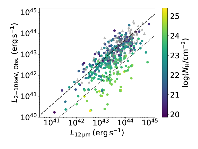
Comparing the observed X-ray 2–10 keV luminosities () to the luminosities (), we see in Figure 1 that unobscured Swift/BAT AGNs tend to follow the relation between the intrinsic (unabsorbed) 2–10 X-ray and nuclear luminosities (dashed black line) established by Asmus et al. (2015), whereas obscured AGNs appear X-ray suppressed when compared to . This decrease in compared to with increasing column density is expected, of course, since the X-ray emission will suffer greater attenuation than the mid-IR emission, and we color code the data in Figure 1 according to the column densities adopted in Section 2. As a population, CT AGNs are generally the furthest offset from the Asmus et al. (2015) relation, exhibiting luminosity ratios of log(/ (this was previously discussed in, e.g. Alexander et al., 2008); we plot this ratio between log() and log() as a dotted black line in Figure 1. As has been done in previous works (e.g. Alexander et al., 2008; Goulding et al., 2011; Asmus et al., 2015), we can use this ratio between and as a diagnostic tool to differentiate between less obscured and heavily obscured or CT AGNs.
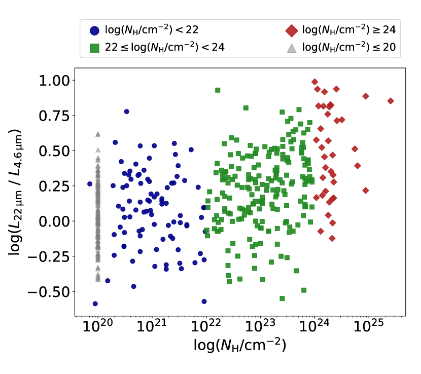
Ratios of two mid-IR luminosities, sufficiently separated in wavelength, could exhibit the same trend as is observed for the / ratio, in that the shorter wavelength mid-IR emission could appear suppressed compared to the longer wavelength emission due to the obscuring material surrounding the AGN. We test a new diagnostic tool based on the ratio of the WISE to luminosity (/) in Figure 2, and we find that the logarithmic ratio increases with column density, with the most significant increase in WISE ratio corresponding to the highest column densities (although with significant scatter). For example, we find a mean luminosity ratio and 1- uncertainty of log(/ for AGNs with log(, whereas we find a mean ratio and 1- uncertainty of log(/ for unobscured AGNs with column densities log(. This suggests that WISE colors can also be used as a diagnostic tool for identifying heavily absorbed AGNs.
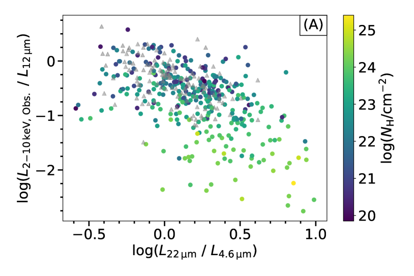
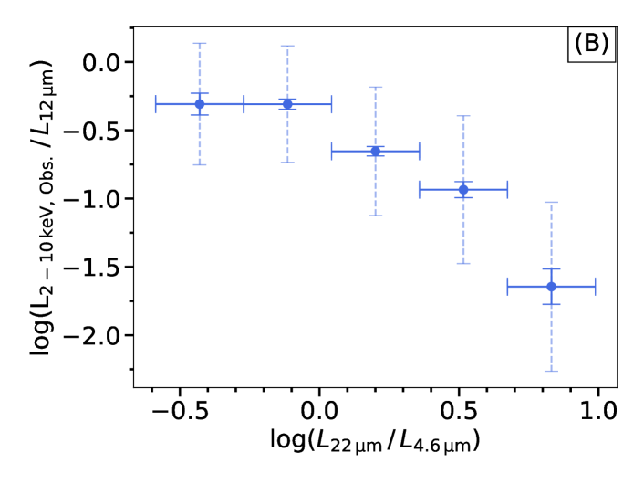
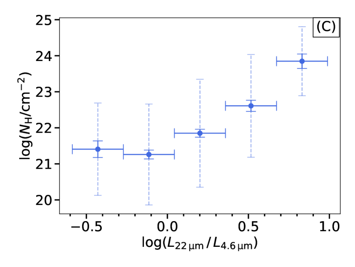
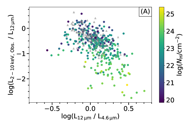
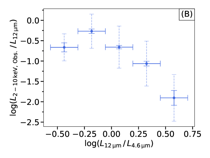
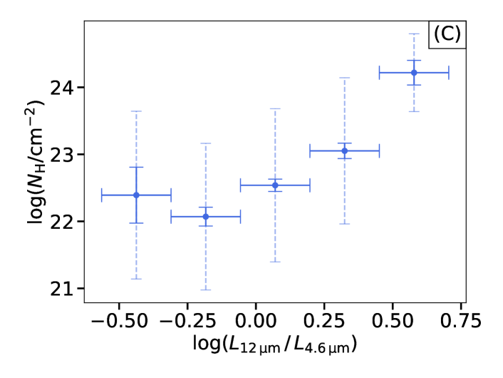
We combine the / and / ratio diagnostics in Figure 4, plotting the two diagnostic ratios against one another in Panel A and color coding the data points by column density on the auxiliary axis. As the column density increases, the AGNs tend to exhibit lower values of / and higher values of /, and thus we find that the most heavily obscured AGNs predominantly occupy the lower right portion of the parameter space (i.e. the largest X-ray deficits and highest / ratios). In Panel B of Figure 4 we show this same result after binning the data by /. In Panel C we bin by / and examine the scatter in the column density by bin; we notice a positive correlation between the column density and the mid-IR luminosity ratio. All solid error bars in Panels B and C represent the standard error of the mean while dashed error bars represent the standard deviation computed for the respective bin. Considering these three panels together, we may define a parameter space using the / and the / luminosity ratio, which could be used to identify the most heavily absorbed AGNs. We repeated this analysis for an alternative WISE luminosity ratio of / and found very similar results (see Figure 4). We explored several AGN selection methods to potentially mitigate or at least account for the scatter observed, which we discuss in the Appendix. Ultimately, we did not apply any selection criteria to our sample of Swift/BAT AGNs during the analysis described below. Of important note, however, is the interesting result that the correlation between the mid-IR color and holds true for both WISE (selected via ; Stern et al., 2012) as well as non-WISE AGNs.
3.1 A Relation for as a Function of /
Since the / ratio is known to correlate with obscuring column (e.g. Ichikawa et al., 2012; Asmus et al., 2015; Yan et al., 2019), we derived an expression to describe this relationship using the Swift/BAT sample studied here. Note that, in contrast to Asmus et al. (2015) (see Section 4.2 for further details), we do not exclude sources with log( from the fitting process.
For our fitting process, we incorporate the luminosity ratios and the associated uncertainties. We pull the uncertainties in the mid-IR fluxes from Ichikawa et al. (2017) and Ichikawa et al. (2019); while uncertainties in the observed X-ray luminosities were not available in the Ricci et al. (2017a) catalog, we conservatively adopt uncertainties of log( for AGNs with log( and log( for AGNs with log(. In order to take into account the asymmetric uncertainties associated with log() and log(/), we employed the following Monte Carlo fitting routine:
-
1.
Bootstrap: To fully account for the effect of outliers, we generated a new data set as a sample of the original, allowing repeats.
-
2.
Monte Carlo: For each point in the bootstrapped data set, we generate a new point given the uncertainties in log() and log(/). We incorporate asymmetric error bars by randomly drawing from a Gaussian distribution separately for the negative and positive error bars. For upper limits in log()333Note there are no limits for log(/)., we generate a new point using a uniform distribution from the limit to an arbitrarily small log() value below it. After experimenting a number of different values, each giving similar results, we settled for a lower bound of log() = 19, which is only marginally lower than the smallest log() value through the Milky Way according to the maps by (Kalberla et al., 2005).
-
3.
Orthogonal Distance Regression: We fit each Monte Carlo-bootstrapped data set with a function of the form using orthogonal distance regression (from the Python scipy package odr (Brown et al., 1990, pp. 186; Virtanen et al., 2020). This ensures we account for minimisation in both variables during the fitting procedure.
-
4.
Parameter Estimation: Steps 1 – 3 were performed many times, giving a distribution for the parameters a, b and c. For each parameter we report the percentile and uncertainties derived from the the and percentiles.
The relationship between / and can be expressed as:
| (1) | |||
We plot the Swift/BAT sample and Equation 1 (orange line) in Figure 5. To visualize the uncertainty in this relation, we show the 1000 realizations of the best fit as grey lines.
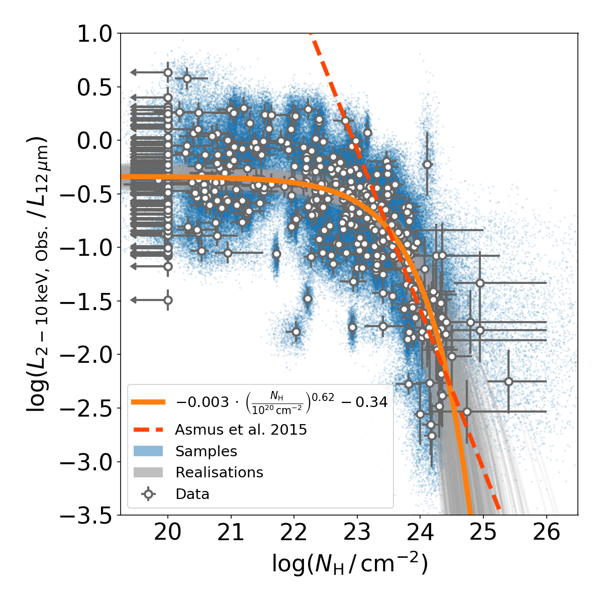
We attempted to fit directly for log() as a function of log(/) but the fitting routine could not successfully converge on a reasonable fit to the data. Instead, we chose to invert Equation 1 to recover the obscuring column density as a function of the X-ray to mid-IR luminosity ratio:
| (2) | |||
To better quantify the uncertainty in log() associated with this relation, we tabulated values of log() and the uncertainty for specific values of log(/), as shown in Table 1. Using the parameter distributions calculated during the MC fitting routine, we derived a distribution of log() values using an expression of the form shown in Equation 2 (inverted from Equation 1) and use the , , and percentiles of the distribution to list the median column density and associated uncertainty for each chosen value of log(/). While strictly empirical, Equations 1 and 2 reproduce the observed trend of decreasing values of log(/) with increasing column density. We do note that this relation is largely insensitive to ratios of log(/, with the relation appearing nearly flat for column densities of log(. Equations 1 and 2 are most effective for obscured AGNs with column densities of log(, and readers should keep this in mind when using these expressions to derive estimates for column densities.
3.2 Relation between and the Mid-Infrared Colors
Given the correlation between / and , as shown in Figure 4, we followed the same fitting procedure as discussed above to develop an expression relating the mid-IR luminosity ratio and . The equation relating these properties can be expressed as:
| (3) | |||
In Figure 6 we plot the Swift/BAT sample and the best-fitting trendline (orange line) along with 1000 realizations of the best fit found during the fitting procedure (shown as gray lines).
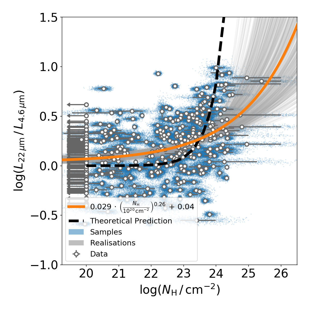
As mentioned in Section 3.1, we attempted to fit directly for as a function of /, but the fitting routine could not successfully converge on a reasonable line of best fit. We therefore simply invert Equation 3 like before to recover the column density as a function of the mid-IR luminosity ratio:
| (4) | |||
In an identical fashion to the calculations in Section 3.1, we tabulated values of log() and the associated uncertainties for specific values of log(/) in Table 2. Equation 4 is not sensitive to values of log(/ and, as in the case of Equation 2, readers should use this relation cautiously and bear in mind that it is really only effective for obscured AGNs with log(.
| log(/) | log() |
|---|---|
| 0.0 | |
| 0.1 | |
| 0.2 | |
| 0.25 | |
| 0.3 | |
| 0.4 | |
| 0.5 | |
| 0.75 | |
| 1.0 |
.
3.3 Diagnostic Regions for Heavily Absorbed AGNs
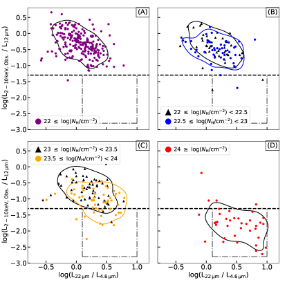
The correlations between /, /, and discussed above suggest that these relationships may be combined to help differentiate between Swift/BAT AGNs according to the levels of obscuration. We probed this potential diagnostic for heavily absorbed AGNs by plotting / vs. / and binning the full sample by absorbing column as shown in Figure 7. The sample was divided into four bins in obscuration corresponding to:
-
•
unobscured
[, Panel A] -
•
Compton-thin “lightly obscured”
[, Panel B] -
•
Compton-thin “moderately obscured”
[, Panel C] -
•
“heavily obscured” to Compton-thick
[, Panel D]
We also split the two Compton-thin bins into two sub-bins each in increments of log(, as summarized in Table 3.
Contours were computed for each bin and/or sub-bin and in each case are designed to encompass of the population of each respective bin. The binned subplots shown in Figure 7 demonstrate much more clearly that, in general, the heavily obscured sources (Panel D) tend to occupy a separate region of space than the unobscured (Panel A) or Compton-thin ‘lightly obscured’ (Panel B) sources. While there is some overlap between the CT and Compton-thin ‘moderately obscured’ populations, this is predominantly due to Compton-thin ‘moderately obscured’ sources with . In light of this, appropriate selection criteria can be used to construct diagnostic regions in this parameter space which separate heavily obscured and less obscured AGN populations. Here we define the completeness of selection criteria as ‘the fraction of true heavily obscured AGNs selected,’ while we define purity as ‘the fraction of selected AGNs which are heavily obscured,’ i.e. the fractional contribution of heavily obscured AGNs to a diagnostic region. These definitions can be extended in an analogous fashion to the other column density bins.
Defining a horizontal cut in this parameter space:
| (5) |
which is shown as a black dashed line in Figure 7, provides a simple yet robust method of differentiating between the most heavily obscured AGNs and less obscured AGNs in the Swift/BAT sample. We report the sample statistics for this cut in Table 3. To derive the population statistics for Table 3 (and all percentages quoted hereafter), we calculated the median ( percentile) value for each population in question, while the uncertainties on the fractions are the and quantiles of a binomial distribution, all computed following Cameron (2011). The criterion in Equation 5 yields completeness for the heavily obscured AGNs, a % pure sample, and a mean column density of log( for the diagnostic region. It is important to note that the majority of impurities selected with Equation 5 arise from AGNs with column densities ; the diagnostic region is in fact % pure for AGNs with and suffers minimal impurities from AGNs with lower column densities.
| Completeness | Purity | |
|---|---|---|
| Completeness | Purity | |
|---|---|---|
In a similar fashion, we could define a vertical cut based on the WISE colors in this space:
| (6) |
and while this criterion also yields a highly complete sample (%) of heavily obscured AGN, the selected sample is only % pure for heavily obscured AGNs and is greatly contaminated by moderately obscured, lightly obscured, and even unobscured AGNs. This is not at all surprising, given the scatter in the mid-IR ratio as demonstrated in Figures 4 and 5. Mid-IR selection alone is therefore not sufficient when attempting to select both a highly complete and fairly pure sample of heavily obscured sources.
Next we defined a slightly more stringent box region (gray dash-dotted line and black dotted line in Panels A–D of Figure 7), which encompasses the majority of the most heavily absorbed sources with minimal overlap with the unobscured and Compton-thin bins, using the following relations:
| (7) | |||
We report the population statistics for this diagnostic box in Table 5. This box offers a completeness of for the heavily obscured AGN population, a pure sample, and a mean column density of log(. As with Equation 5, the largest source of impurities within this region are AGNs with ; the region is % pure for AGNs with log( and suffers few impurities from AGNs of lower column densities.
| Completeness | Purity | |
|---|---|---|
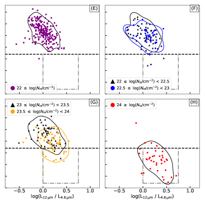
We repeated this analysis for the alternative / luminosity ratio, and we show the contoured populations binned by column density along with an alternative diagnostic box for heavily absorbed sources in Panels E–H of Figure 7. We construct this box with the following relations:
| (8) | |||
and we find that this box yields a completeness of for heavily absorbed AGNs, a purity of %, and a median column density of log(. Again, AGNs with column densities contribute the most to the impurity of the sample, while AGNs with lower column densities do not contribute as significantly.
The diagnostic metrics defined above — developed using the well-constrained X-ray and mid-IR properties previously found for Swift/BAT AGNs (e.g. Ricci et al., 2017a; Ichikawa et al., 2017) — carve out parameter spaces that yield fairly complete and fairly pure samples of heavily obscured AGNs, offering an efficient and effective method for identifying heavily obscured or CT AGN candidates, particularly in large samples of AGNs.
4 Discussion
4.1 The physical origin of the trend in WISE ratios as a function of
The observed trend of the and WISE ratios increasing with column density can be readily understood from dust absorption and emission properties and basics of the radiation transfer. For media optically thin to the mid-IR radiation, the shape of the resulting SED will be determined predominantly by the dust temperature and its gradient throughout the dusty structure. If the dusty medium is optically thick to its own radiation, the outgoing emission will be reshaped due to a number of reasons: (i) Warm dust emission at shorter wavelengths will be absorbed and re-emitted at longer wavelengths. (ii) Dust emission at shorter wavelengths will suffer more extinction than the long-wavelength emission, owing to the wavelength-dependent extinction for typical AGN dust (Laor & Draine, 1993). (iii) Warm dust emission originates closer to the inner rim of the torus, while colder emission originates farther out. As a consequence, longer wavelength mid-IR radiation has to travel a shorter path through the dust before reaching us and thus, suffers even less extinction than the emission of shorter wavelengths. These three effects result in an increased ratio of longer-to-shorter wavelength mid-IR emission and scale with the column density of the medium through which the X-ray radiation is traversing. (iv) Additionally, a disk-like molecular structure in hydrostatic equilibrium is expected to have a vertical gradient (Hönig, 2019). In this case, the observed trend of increasing WISE ratios with increasing can be explained simply as an inclination effect: the closer our viewing angle is to the equator, the higher is the column density along the line-of-sight and, at the same time, the dust emission becomes “redder”. All these effects contribute to the observed trend of increasing WISE ratios with and also explain why the effect is more pronounced in the than at luminosity ratio (for illustration, see torus model SEDs in, e.g., Hönig & Kishimoto, 2010; Stalevski et al., 2012).
There are a few caveats: The dust emission is often degenerate, as SEDs of similar shape can be produced by different combinations of the geometrical and physical parameters of the torus, some of which can conspire to work against or hide the trend in luminosity ratios. However, the above reasoning should hold in general since it relies on universal radiative transfer effects. Another deviation can be introduced by the presence of silicate dust grains which exhibit a strong increase of absorption efficiency around and . The apparent strength of these features appear in an SED depends on several factors, including the amount of silicates, grain size distribution, and radiative transfer effects.
We illustrate these effects in Figure 6 with a black dashed line, which represents a theoretical expectation for a very simple model: monochromatic radiation passing through a homogeneous screen of dust. For this example, we assumed a typical Galactic interstellar dust mixture of silicates and graphite (e.g., Stalevski et al. 2016). The grain size distribution are from Mathis et al. (1977) and optical properties from Laor & Draine (1993) and Li & Draine (2001). The conversion between the optical depth and assumes Galactic relation between extinction and column density found by Predehl & Schmitt (1995). We see that the theoretical curve is following the trend of the data at lower column densities, but is reaching the breaking point sooner. This is because the simple dust screen model does not account for a number of radiative transfer effects (self-consistent absorption and re-emission of the thermal IR radiation), which together with geometry of the dusty medium and orientation shape the resulting SED, and thus, the observed trend of luminosity ratios with column density.
4.2 Comparison to Asmus et al. (2015)
Using sub-arcsecond resolution mid-IR observations – which enabled the isolation of the nuclear mid-IR emission () – Asmus et al. (2015) found a significant correlation between and for 53 AGNs with reliable X-ray observations and column densities log(, which was expressed as (see Equation 6 in Asmus et al., 2015):
| (9) | |||
This expression is plotted in Figure 5 (dashed red line) along with our Equation 2 (solid orange line) and the Swift/BAT sample. Along with values of log() derived using Equation 2 in Section 3.1, we use the relation from Asmus et al. (2015) to derive values of log() and the uncertainties for specific values of log(/) in order to compare to our own results. Despite the fact that Asmus et al. (2015) removed AGNs with and utilized subarcsecond-resolution mid-IR emission (whereas in this work we utilized lower angular resolution mid-IR photometry for the Swift/BAT sample), it does appear that the two relations generally agree (within the uncertainties) for ratios of (/. The two relations differ more severely for higher ratios of log(/), though this is expected due to (1) the wide range of ratios that unobscured AGNs exhibit and (2) the fact that our relation turns over to account for less obscured sources while the Asmus et al. (2015) relation does not take into account less obscured sources.
4.3 Diagnosing Column Densities with Uncertain Dust Heating Sources
While the diagnostic boxes defined in Section 3 provide a reliable way to identify the most heavily obscured AGNs, star formation activity can contribute non-negligibly to the mid-IR colors of an AGN host. The mid-IR colors assumed to originate from the AGN itself could therefore be overestimated without performing detailed spectral energy decomposition (SED) fitting to differentiate between the AGN and star formation contributions to the mid-IR continuum. Furthermore, Satyapal et al. (2018) demonstrated, using Cloudy (Ferland et al., 2013, 2017) radiative transfer models, that heavily obscured star formation activity can actually mimic the mid-IR colors of AGNs. These two points suggest that our diagnostic boxes defined in Section 3 may (1) misdiagnose the column density of an AGN if significant star formation is present, as the contaminating stellar emission could lead to much redder colors than the AGN intrinsically exhibits, or (2) mislead us to think an AGN is present in cases where the dominant dust heating sources are actually stellar-related rather than AGN-related (Satyapal et al., 2018). To investigate this potential contamination of the diagnostic boxes, we constructed a catalog of optically-selected galaxies whose optical spectroscopic line ratios suggest star formation dominates the observed emission, and we examined methods – for example mid-IR or X-ray selection criteria – through which this contamination could be mitigated.
Beginning with the MPA-JHU catalog of galaxy properties (from the SDSS data release 8, Aihara et al., 2011), we first selected systems with redshifts and included only systems which are classified as star forming systems (“BPTClass” = 1) based upon their Baldwin, Phillips, Telervich (BPT; Baldwin et al., 1981) optical spectroscopic emission line ratios. We also removed any systems with QSO and AGN flags within the “TARGETTYPE,” “SPECTROTYPE,” and “SUBCLASS” columns, and then narrowed the sample to only systems with WISE counterparts and X-ray counterparts from the 4XMM point source catalog (Webb et al., submitted). These criteria yielded a full parent sample of 448 galaxies which we assume are ‘purely’ star forming systems based upon optical spectroscopic measurements. We make no distinction between morphological classes of galaxies.
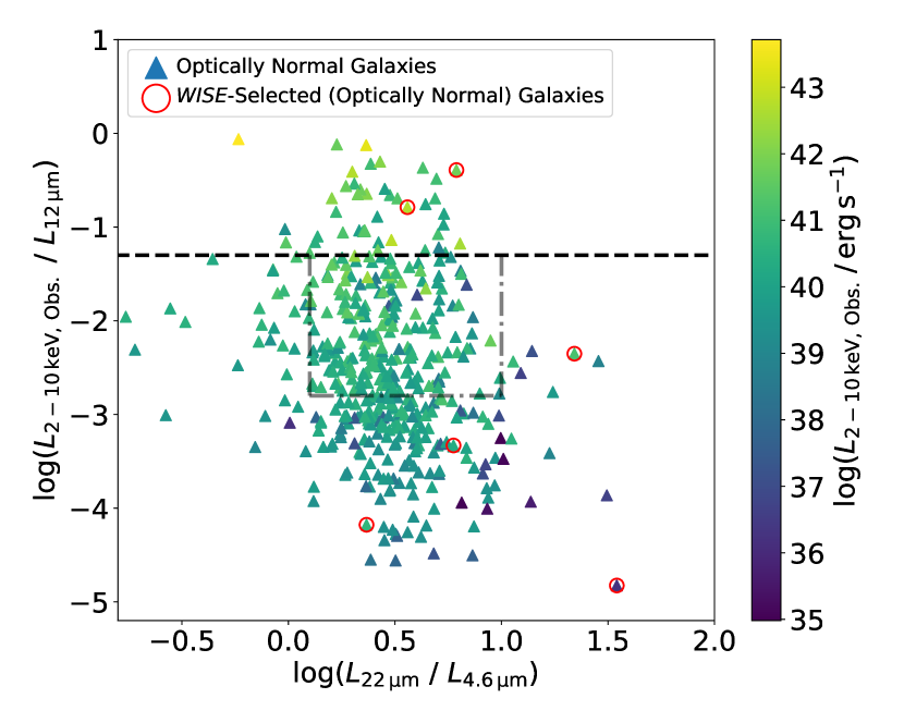
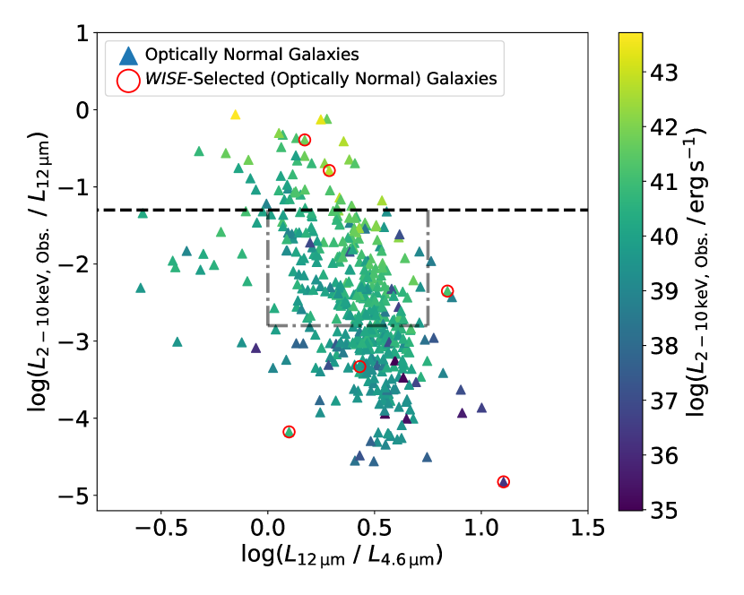
We plot our population of optically-selected star forming galaxies (color coded according to the observed X-ray luminosity) along with the / and / diagnostic boxes in Figure 8. While star formation dominated galaxies tend to exhibit lower ratios of log(/) than the majority of the Swift/BAT sample, they do tend to exhibit similar X-ray deficits as well as / and / mid-IR colors as those exhibited by the heavily obscured Swift/BAT AGNs; in fact, of this star forming population overlaps the / diagnostic region, while of the population overlaps the / region. We therefore caution that this diagnostic is emphatically not designed to differentiate between star forming and AGN-dominated systems and should not be used as a diagnosis of the dominant dust heating source. Nevertheless, the contamination from optically-selected star forming systems can be mitigated through the use of reliable mid-IR and X-ray selection criteria traditionally used for identifying AGNs.
We applied the two band WISE AGN selection cut (–) from Stern et al. (2012) to the sample of star forming galaxies, which removed all but six systems (red empty circles, shown in Figure 8). As expected, requiring traditional mid-IR AGN selection criteria eliminates virtually all contamination by optically-selected star forming systems within the diagnostic boxes. While six star forming galaxies (% of the total population) succeed in meeting the Stern et al. (2012) cut, these do still fall outside of our diagnostic boxes.4444/6 sources do fall below our cut in /: (1) a compact star forming region in a galaxy Mpc away, and (2) a galaxy at , (3) a pair of merging galaxies at , (4) a pair of merging galaxies which actually host a candidate dual AGN at (Pfeifle et al., 2019). Thus, use of mid-IR AGN selection tools could be used to avoid misdiagnosing the dominant photoionization process of the sources within the diagnostic regions. However, it is important to bear in mind that the relation between /, / (and /), and holds true for both WISE and non-WISE selected AGNs (see Appendix), and therefore requiring a WISE cut could in general remove true AGNs as well as star forming systems. For example, imposing the – cut on the Swift/BAT sample examined in this work would remove 240 systems (or % of the parent sample of 456 AGNs); in the parent sample of 456, there are 71 AGNs which possess column densities in excess of cm-2, and 40 of these would be removed with this mid-IR cut.
We also found that requiring an observed X-ray luminosity of erg s-1 removes nearly all of the optically star forming population from the diagnostic region (5 galaxies, or %, remain within the / diagnostic box), though this method must also be used judiciously to avoid removing heavily obscured AGNs, which could exhibit lower X-ray luminosities.
Ideally, the usage of this diagnostic should be limited to systems whose dominant photoionization processes are unambiguous or for which detailed SED fitting can be performed to differentiate between AGN and host emission. Otherwise, we recommend proceeding cautiously, taking into account the various caveats outlined above to avoid inaccurate estimations of the obscuration along the line-of-sight.
4.4 Mid-IR Emission Contributions from Galaxies Hosting Obscured AGNs
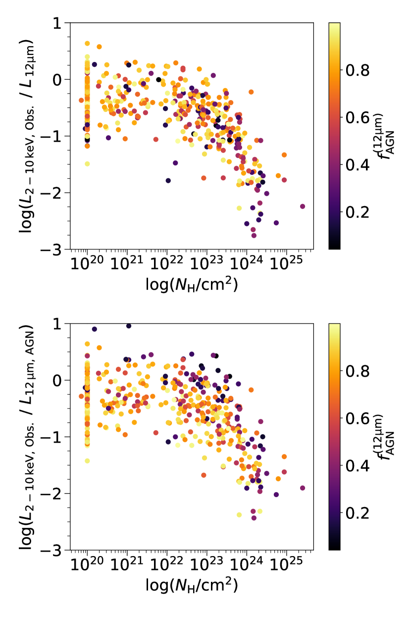
The realization in Section 4.3 that optically star forming galaxies, which presumably do not host AGNs, can exhibit luminosity ratios similar to those exhibited by more heavily obscured or CT Swift/BAT AGNs raises the intriguing point of how much host galaxies may contribute to the observed luminosity ratios derived for the Swift/BAT AGNs. Figure 9 shows the log(/) and log(/) ratios of the Swift/BAT AGNs and is color-coded according to the fractional contribution by the AGN to the observed 12 emission () derived through detailed SED fitting in Ichikawa et al. (2019). While host-dominated systems at 12 () can be found across this parameter space, a significant fraction (%, 22 out of 51) of AGNs within the diagnostic region (Equation 7) reside in host-dominated systems. This suggests that the host galaxies could contribute significantly to the observed mid-IR colors of the heavily obscured AGN population in particular, presumably via dust emission heated through star formation.

Ichikawa et al. (2019) provided decomposed logarithmic AGN 12 luminosities for the Swift/BAT AGNs, which we can use here to examine how the log(/) ratios may change if we use the AGN 12 luminosity () instead of the total observed 12 luminosity (). Figure 10 (top panel) shows that host-dominated systems are predominantly occupied by AGNs with log(; half of the CT Swift/BAT AGNs reside in host dominated systems. After recalculating the luminosity ratio using instead (bottom panel), host-dominated systems exhibit a shift toward higher luminosity ratios, with an average difference in ratio of log(/ for AGNs with , although we note that these shifts are not limited only to heavily obscured AGNs. Here we have assumed that the X-ray emission is AGN-dominated, rather than host-dominated; in reality, if some portion of the X-ray emission is due to the host as well, the observed ratio shifts will not be as large.
Figure 9 demonstrates that host galaxies do indeed contribute significantly to the diagnostic ratios probed in this work, at least for systems in which the host dominates the mid-IR emission at 12 . In these cases, the host contribution to the mid-IR leads to a perceived larger X-ray deficit for the AGN at a given column density. It does appear, though, that generally this effect actually works in our favor when attempting to identify CT AGNs, as these more severe X-ray deficits and presumably ‘redder’ mid-IR colors aid in separating this population from less obscured populations in color space. Decomposed AGN 22 and 4.6 luminosities were not included in Table 1 of Ichikawa et al. (2019) and therefore could not be examined in a similar fashion here. While it is beyond the scope of this paper, an analysis of the interplay between the mid-IR colors, host galaxy emission, and AGN emission with regard to the selection diagnostics presented in this work should be performed more rigorously in a future study.
4.5 Comparison to Kilerci-Eser et al. (2020)
In a very recent study, Kilerci-Eser et al. (2020) selected a subsample of the 105 month Swift/BAT catalog (Oh et al., 2018) and proposed a new selection method for CT AGNs using mid-IR and far-IR photometry. They report, as we do here in Section 3 of this study, a shift in infrared colors (specifically mid-IR and far-IR) toward ‘redder’ colors with increasing column density, and they define a physically motivated color-color diagram (see Figure 11, henceforth , in Kilerci-Eser et al., 2020) and selection method using the []–[] and []–[] colors. Of the 32 CT Swift/BAT AGN for which there exists the relevant photometry, this selection criteria identifies four CT AGNs (a success rate of ). However, it is evident from that these color cuts cannot reliably distinguish between unobscured, obscured, and CT AGNs, as the AGNs from these three different obscuration bins largely occupy the same []–[] and []–[] parameter space. In the case of Swift/BAT, the color-color criteria proposed by Kilerci-Eser et al. (2020) yields a far lower success rate of identifying heavily obscured and CT AGNs than the criteria set forth in this work (e.g. Equations 7 and 8; see Tables 3, 5, and 6).
To further test their diagnostic, they applied this color selection criteria to the AKARI infrared galaxy catalog developed in Kilerci Eser & Goto (2018), which contains over 17,000 galaxies, and recover one known CT AGN (NGC 4418, e.g. Sakamoto et al., 2013).555The selection criteria also recovers two other sources: NGC 7714, an unobscured AGN (Gonzalez-Delgado et al., 1995; Smith et al., 2005), and NGC 1614, which has no clear evidence of an AGN (e.g. Xu et al., 2015; Pereira-Santaella et al., 2011; Herrero-Illana et al., 2014). The remainder of the infrared galaxy sample of Kilerci Eser & Goto (2018) is represented with blue contours in that partially overlap a significant number of Swift/BAT CT, obscured, and unobscured AGNs, suggesting that some portion of these infrared galaxies may in fact host heavily obscured AGNs. Despite finding a few cases of CT AGNs between the Swift/BAT and Kilerci Eser & Goto (2018) samples, the diagnostic criteria set forth in Kilerci-Eser et al. (2020) does not appear to provide a complete or reliable (see Section 5.4 of Kilerci-Eser et al., 2020) method of selecting CT AGNs.
As an additional comparison between our selection method and that proposed by Kilerci-Eser et al. (2020), we turned our attention to the infrared galaxy catalog from Kilerci Eser & Goto (2018). We matched this sample to the AllWISE catalog and the 4XMM DR9 XMM-Newton Serendipitous Source Catalog (Webb et al. submitted), using a match radius of 10′′ for each, which yielded a sample of 401 local () infrared galaxies with XMM-Newton and WISE detections. In Figure 11, we show the resulting sample of infrared galaxies (red stars), along with our diagnostic criteria from Equations 5 and 7. As in Section 4.3, it is impossible to discern whether or not any of these galaxies host AGNs without a reliable method for removing star formation dominated systems. We tried four different mid-IR AGN selection criteria, defined in Jarrett et al. (2011), Stern et al. (2012), Assef et al. (2018), and Satyapal et al. (2018) (with the understanding that some heavily obscured AGNs will be missed with this simple approach), and in all four cases we recover a significant number of candidate heavily obscured or CT AGNs. We show mid-IR AGNs selected as a result of the Stern et al. (2012) cut in Figure 11 (blue squares); these candidate CT AGNs likely inhabited the blue contoured prominence that overlapped the Swift/BAT AGNs in , but were missed due to fact that they did not satisfy the criteria proposed by Kilerci-Eser et al. (2020).

Table 7 in the Appendix lists the 36 candidate CT AGNs selected from Kilerci Eser & Goto (2018) using the / diagnostic region and at least one of the mid-IR selection cuts listed above. We include in the table the source coordinates, redshifts, luminosity ratios, and alternative identifiers, and we also categorize the column densities of the sources (using the column density bins defined in Section 3.3) based upon any available measurements in the literature. Of the candidates that have inferred or directly measured column densities in the literature (24/36), we find eight CT AGNs, six moderately obscured AGNs, two lightly obscured AGNs, and three unobscured AGN, while a remaining five AGNs have conflicting measurements of in the literature (all five of which have been reported as CT at least once in the past).666There are other moderately and heavily obscured WISE AGNs in this sample which did exhibit log(/) but fall outside of our more stringent diagnostic region. Therefore, we conclude that our diagnostic criteria proposed in Equations 5, 7, and 8 offer a more reliable method for identifying candidate CT AGNs than the mid-IR to far-IR color criteria proposed by Kilerci-Eser et al. (2020).
In light of Section 4.4, we caution that some portion of these AGNs may not dominate the observed emission and, therefore, may exhibit larger X-ray deficits and redder mid-IR colors than might be expected for the AGN alone due to additional mid-IR contributions from the host galaxy.
4.6 Diagnosis of in the XXM-XXL Field
To test the power of our absorption diagnostic, we turn our attention to its application in the XMM XXL North field (Pierre et al., 2016, 2017). Menzel et al. (2016) presented a rigorous multiwavelength analysis of 8445 X-ray sources detected by XMM-Newton in an 18 deg2 area of the XMM XXL North field (hereafter XXL-N), with a limiting flux of erg cm-2 s-1, providing optical Sloan Digital Sky Survey (SDSS) and mid-IR WISE counterparts to the XMM-Newton sources. In a complementary investigation, Liu et al. (2016) presented a thorough X-ray spectral analysis of the 2512 XXL-N AGNs, deriving the spectral properties (e.g. photon index , , ) for those AGNs using a Bayesian statistical approach contained within the Bayesian X-ray Astronomy (BXA) software package (Buchner et al., 2014).
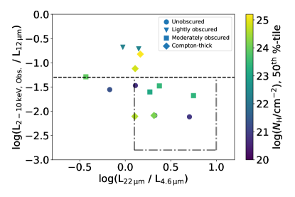

We combined the catalogs from Menzel et al. (2016) and Liu et al. (2016) to obtain the observed 2–10 keV luminosities and mid-IR WISE magnitudes, from which we derived the relevant luminosity ratios examined in Section 3. Initially we limited the XXL-N sample to only local () AGNs, and as with the Swift/BAT AGNs, we did not employ any mid-IR or X-ray selection criteria. We plot the resulting luminosity ratios of the low redshift AGNs from the XXL-N field in the left panel of Figure 12 along with our / diagnostic box (Equation 7) and horizontal cut in / (Equation 5). The data and auxiliary axis in Figure 12 are color coded to represent the derived -percentile values from the Liu et al. (2016) catalog and the markers denote the obscuration bin for each AGN. In the right panel of Figure 12 we plot the / ratio against the derived log() values from Liu et al. (2016), where the error bars represent the and percentiles and the data points use the same marker and color scheme as the left panel. A dearth of low redshift AGNs in the XXL-N field is immediately apparent, and while it appears that most of the more obscured AGNs do exhibit “redder” colors, there is some overlap in / ratios exhibited by AGNs of starkly different obscuration bins, e.g. heavily obscured and unobscured AGNs. Unfortunately, we cannot draw definitive conclusions about the reliability of our diagnostic for the XXL-N field with such poor AGN statistics.
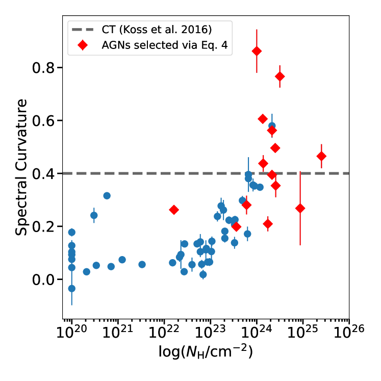
We repeated this analysis for the entire sample of XXL-N AGNs, breaking the sample into redshift bins of each. While a small number of obscured AGNs overlap with the diagnostic region defined by Equation 7, the majority of the heavily absorbed AGNs still occupy the same parameter space as the Compton-thin and unobscured AGNs, even in the local () redshift bin, in stark contrast to the results found with the Swift/BAT AGNs. We find a very similar result when examining the / diagnostic ratio. Due to the fact that at higher redshift the / and / diagnostics do not correspond to the same wavelength ranges as they do at local redshifts, we then turned to the luminosity ratio of . Yet again the heavily absorbed AGNs generally occupy the same parameter space as unobscured AGNs. The spectral curvature method (Koss et al., 2016) may provide a more effective means of selecting heavily obscured AGNs at higher redshift in the XXL-N field, and indeed Baronchelli et al. (2017) demonstrated its effectiveness in selecting high redshift () CT AGNs in both the Chandra Deep Field South and the Chandra COSMOS legacy survey.
There are a few explanations for why the luminosity ratios of the XXL-N AGNs do not as clearly differentiate between obscuration levels like that seen for the Swift/BAT AGNs. For one, there may simply not be enough local redshift XXL-N AGNs for a proper statistical comparison to the results found for the Swift/BAT AGNs. Secondly, it is possible that the chosen redshift bins are not fine enough and we are including AGNs across too large of redshift ranges. After splitting the bin into five sub-bins, however, we find the same result as before: the unobscured and heavily obscured AGNs coexist within the parameter space.
Another explanation lies in the reliability of the results of the X-ray spectral fitting performed in Liu et al. (2016): while the Bayesian statistical framework employed in that work is a powerful method for constraining the spectral properties for AGNs with low counts, our results suggest that the column densities derived for the AGNs may still be inaccurate due to the low counts acquired. For example, for all AGNs detected in the bin, the median number of counts detected in the epic pn and in the two epic mos detectors is only and counts, respectively. Furthermore, identification of Compton-thick AGNs via XMM-Newton spectroscopy is quite difficult due to the softer X-ray passband (0.3-10 keV) probed with the XMM-Newton imaging. It can be very difficult to distinguish between the scenario in which the source is heavily obscured, and the X-ray emission is dominated by reprocessed radiation from the circumnuclear material, and that in which the source is unobscured but the emission is dominated by relativistic reflection from the accretion disk when using low signal-to-noise X-ray spectra alone due to the strong model-dependent degeneracies involved (see e.g., Gandhi et al., 2009, Treister et al., 2009). Our mid-IR ratio predictions for the highest X-ray column densities can hence be very complementary to help classify sources in which unobscured and obscured reflection models can fit an observed X-ray spectrum equally well.
Future, deeper XMM-Newton or NuSTAR follow-up observations could improve upon the current photon statistics and could provide robust constraints on the column densities for at least the local XXL-N AGNs which lie within the diagnostic boxes. For now, we identify these systems as candidate heavily obscured or CT AGNs, and we list their spectral properties in Table 8.
5 Conclusions
Using the well-studied Swift/BAT sample of ultra hard X-ray selected AGNs, we have presented an analysis of the AGN / luminosity ratio and two different mid-IR luminosity ratios: / and /. Using the well constrained X-ray (Ricci et al., 2017a) and mid-IR (Ichikawa et al., 2017) properties of the Swift/BAT AGNs, we probed the utility of these luminosity ratios as tools for inferring line-of-sight column densities and identifying the most heavily obscured AGNs in the local Universe (. We summarize the results of our analysis as follows:
- •
-
•
We have demonstrated that unobscured and heavily obscured AGNs tend to exhibit different /, /, and
/ luminosity ratios. All three of our diagnostic regions (Equations 5, 7, and 8) identify (in general) the most heavily absorbed AGNs, with average column densities of for each defined parameter space. These regions are all % complete and % pure for AGNs with log(. The greatest impurities arise due to AGNs with ; these regions are % pure for AGNs with . -
•
While optically star forming systems can fall within our diagnostic regions, this contamination can be virtually eliminated via mid-IR or X-ray selection criteria. Such selection criteria should be used judiciously to avoid removing non-mid-IR AGNs. These diagnostic regions should not be used to differentiate between AGNs and galaxies dominated by star formation.
-
•
Swift/BAT AGNs which do not dominate the total observed emission tend to exhibit redder colors and larger X-ray deficits with increasing column density, suggesting that host galaxy contributions to at least the mid-IR emission can be a significant factor in the luminosity ratios examined here, particularly in the case of mildly obscured and CT AGNs selected with our diagnostics. However, it appears that this effect actually aids in the identification of CT AGNs, as the host contributions result in a larger separation in color space between less obscured and more obscured AGNs.
-
•
We find that the selection criteria proposed here are more reliable at identifying obscured and CT AGNs than the mid-IR and far-IR selection criteria proposed by Kilerci-Eser et al. (2020). We identify several known obscured and CT AGNs, as well as several candidate CT AGNs, within the IR galaxy catalog of Kilerci Eser & Goto (2018) (see Table 7).
-
•
We applied our diagnostics to the XMM-Newton XXL-N field and found, in contrast to Swift/BAT AGNs, that obscured and unobscured XXL-N AGNs do not appear to exhibit distinctly different luminosity ratios. This disparity could be due to poor photon statistics or the softer X-ray energies probed for the XXL-N AGNs, which could lead to inaccurate column density values. Although, given the small number of XXL-N AGNs and the large errors associated with several values, this comparison should be viewed with caution.
Identifying heavily obscured AGNs remains an important yet difficult task, though the study of such AGNs is an important step in the development of our understanding of the evolution of AGNs. In a future study, we could expand our analysis to include diagnostic regions appropriately modified to differentiate between unobscured and heavily obscured sources at higher redshift, although it is difficult to speculate at the moment how the emission ratios may change with redshift, as both star formation activity and AGN activity are expected to increase with redshift.
The selection criteria presented here offers a complementary approach to the spectral curvature method developed in Koss et al. (2016), which is very effective at selecting heavily obscured AGNs at local-, with the caveats that one must already have hard X-ray ( keV) measurements with NuSTAR or Swift/BAT and that it is most effective for brighter AGNs. Softer X-ray missions can only be utilized for higher redshift sources () for which the hard X-ray emission has shifted into the rest frame 10–30 keV passband. The diagnostics presented here, on the other hand, do not require higher energy passbands in order to select local- sources and can take advantage of softer X-ray missions such as Chandra and XMM-Newton. The synergy between these two approaches is best summed up by the fact that they select many of the same sources using different passbands, and that they select heavily obscured AGNs missed by one another (see Figure 15 in the Appendix), yielding a more complete census of heavily obscured Swift/BAT AGNs overall.
The diagnostic regions proposed in this study, as well as the expressions derived relating to the / and / luminosity ratios, could be used to differentiate between unobscured and heavily obscured AGNs in future, large samples of AGNs, such as those now being detected by the eROSITA all-sky survey (Predehl et al., 2010; Merloni et al., 2012). In particular, the eROSITA survey will provide the first all-sky X-ray imaging survey at energies up to 10 keV, yielding a highly complementary catalog to those of other all-sky missions, such as WISE. Future works could cross-match the WISE and eROSITA catalogs and use the diagnostics presented here to identify many more cases of CT AGN candidates, select targets for deeper follow-up multiwavelength observations, and to compute the CT fraction for the future sample, all of which will be crucial in the quest to construct a more complete census of CT AGNs and gain a better understanding of obscured AGNs.
6 Appendix
6.1 Exploring the Origin of the Scatter in the / vs. Correlation
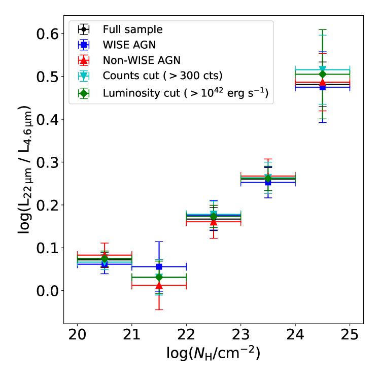
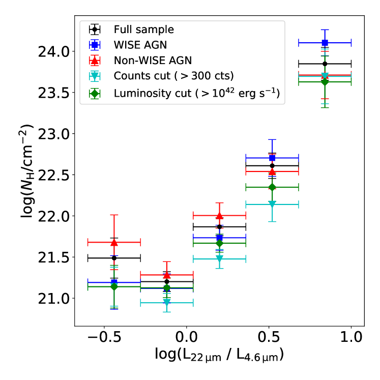
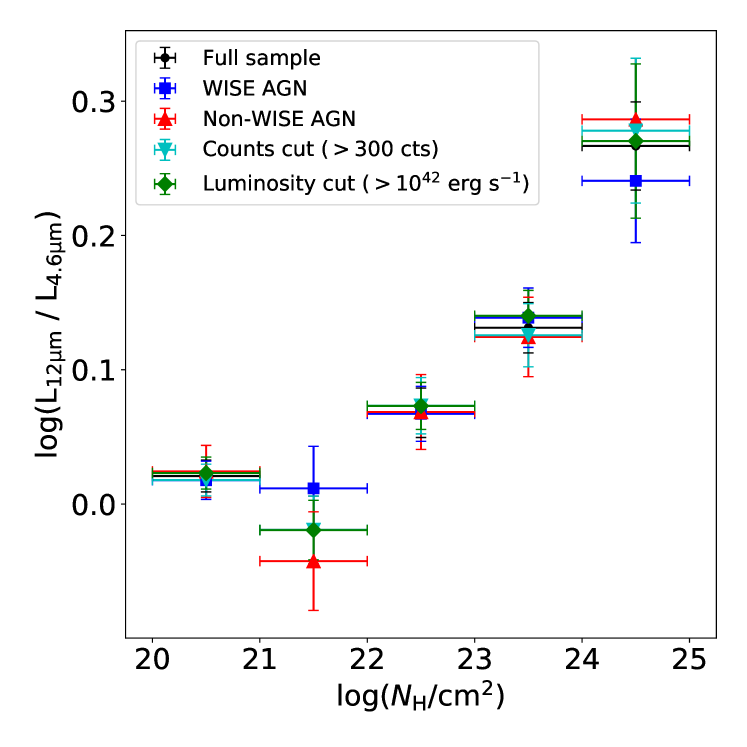
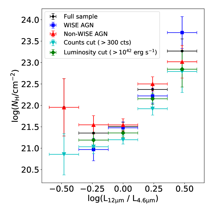
In the process of our analysis, we explored whether any quality cuts or selection cuts could be applied to the data to reduce the scatter observed in Panel A of both Figures 4 and 4. Our parent sample was divided into four sub-samples as shown in Figure 14:
-
•
AGN-dominated systems with – (Stern et al., 2012, blue squares).
-
•
AGNs not selected using the aforementioned WISE cut, i.e. – (red triangles).
-
•
AGNs with spectral counts in the X-ray spectra, which provides a statistically significant number of counts to constrain in the X-ray spectral fitting analysis (Ricci et al., 2017a, inverted cyan triangles).
-
•
AGNs with observed 2–10 keV luminosities in excess of erg s-1 (green diamonds).
In Figures 14 and 14 we compare these sub-samples for the / and / luminosity ratios, respectively, and how they correlate with . The resulting mean values per bin for each different sub-sample are consistent with the values (the error bars represent the standard deviation of each subsample) originally found for the parent sample; interestingly, the observed correlation between WISE color and column density holds for AGNs that satisfy the Stern et al. (2012) criterion as well as AGNs which do not satisfy that criterion. We observe a larger difference in the / ratios when moving to higher column densities than for the / ratios. Additionally, as shown previously in Figure 4, while there is a large amount of scatter in the lowest- bin of the bottom panel of Figure 14, this scatter is likely due to the low number of sources within that bin, and this still does not overlap the bin probing the highest obscuring columns. Due to the consistency between the results for the sub-samples and that found for the parent sample, we do not implement any of these cuts during our analysis.
From Figure 14 and 14, it becomes clear that there a number of WISE AGNs (W1-W2 > 0.8) within the Swift/BAT sample which exhibit extremely red mid-IR colors, with log(/) , suggesting significant obscuration. We tabulate these WISE AGNs in Table 9. Indeed, the majority of these AGNs (18/23) are moderately to heavily obscured with log() , though there are a few exceptions, notably:
-
•
HS0328+0528, an unobscured Seyfert 1.
-
•
IRAS05189-2524, a lightly obscured Seyfert 2.
-
•
2MASXJ09172716-6456271, an unobscured Seyfert 2.
-
•
MCG-1-24-12, a lightly obscured Seyfert 2.
-
•
NGC4253, an unobscured Seyfert 1.
WISE selection based on the cut defined in Stern et al. (2012) is not, however, a necessarily good method for selecting obscured over unobscured AGNs. As we discussed in Section 4.3, 40/71 of AGNs with log() cm-2 in the Swift/BAT sample studied here do not meet a color cut of W1-W2 > 0.8, reinforcing our choice to not invoke such a cut on the parent sample.
| Completeness | Purity | |
|---|---|---|
| AKARI I.D. | RA | Dec | Selection | log | log | Alternate | Obscuration | ||
|---|---|---|---|---|---|---|---|---|---|
| Method | I.D. | Class | Ref. | ||||||
| 0041533+402120 | 10.473 | 40.355 | 0.071 | 3, 4 | 0.62 | -1.52 | Mrk 957 | … | … |
| 0138053-125210 | 24.522 | -12.87 | 0.04 | 1, 2, 3, 4 | 0.47 | -2.47 | IRAS 01356-1307 | Heavily Obscured | 1 |
| 0143576+022059 | 25.991 | 2.35 | 0.017 | 1, 2, 3, 4 | 0.35 | -2.29 | Mrk 573 / UGC 1214 | Heavily Obscured | 2 |
| 0150029-072549 | 27.511 | -7.43 | 0.018 | 1, 2, 3, 4 | 0.64 | -1.44 | IRAS 01475-0740 | Unobscured or Heavily Obscured | 3, 4 |
| 0222435-084305 | 35.682 | -8.719 | 0.045 | 1, 2, 3, 4 | 0.37 | -1.72 | NGC 905 | … | … |
| 0325256-060832 | 51.356 | -6.144 | 0.034 | 4 | 0.36 | -1.45 | Mrk 609 | Unobscured777Despite a lack of broad optical lines, Mrk 609 shows no sign of obscuration at X-ray wavelengths (LaMassa et al., 2014) | 5 |
| 0330407-030814 | 52.670 | -3.138 | 0.021 | 4 | 0.52 | -1.73 | Mrk 612 | Moderately Obscured | 2 |
| 0452447-031256 | 73.186 | -3.216 | 0.016 | 1, 2, 3, 4 | 0.64 | -2.35 | IRAS 04502-0317 | … | … |
| 0453257+040341 | 73.357 | 4.062 | 0.029 | 1, 2, 3, 4 | 0.18 | -1.78 | 2MASX J04532576+0403416 | Moderately or Heavily Obscured | 6, 7 |
| 0518178-344536 | 79.575 | -34.761 | 0.066 | 4 | 0.49 | -1.43 | IRAS 05164-3448 | … | … |
| 0521013-252146 | 80.256 | -25.363 | 0.043 | 1, 2, 3, 4 | 0.36 | -1.44 | IRAS 05189-2524 | Lightly obscured888Based upon current measurements, it is believed that IRAS 05189-2524 is currently lightly obscured, although it is possible that it may have been heavily obscured in the past (Teng et al., 2015). | 8, 7 |
| 0525179-460023 | 81.325 | -46.006 | 0.042 | 1, 2, 3, 4 | 0.42 | -1.56 | ESO 253-3 | Moderately obscured | 9 |
| 0742406+651031 | 115.674 | 65.177 | 0.037 | 1, 2, 3, 4 | 0.49 | -1.58 | Mrk 78 | Heavily or moderately obscured | 10, 7, 11 |
| 0759401+152314 | 119.917 | 15.387 | 0.016 | 4 | 0.41 | -2.74 | UGC 4145 | … | … |
| 0807411+390015 | 121.921 | 39.004 | 0.023 | 4 | 0.83 | -2.04 | Mrk 622 | Heavily Obscured | 7 |
| 0810401+481233 | 122.668 | 48.209 | 0.077 | 3, 4 | 0.74 | -2.11 | 2MASX J08104028+4812335 | Moderately Obscured | 1 |
| 0904011+012733 | 136.004 | 1.458 | 0.054 | 4 | 0.6 | -2.54 | IRAS 09014+0139 | … | … |
| 0935514+612112 | 143.965 | 61.353 | 0.039 | 1, 2, 3, 4 | 0.12 | -2.28 | UGC 5101 | Heavily Obscured | 7, 12 |
| 1010432+061157 | 152.681 | 6.2 | 0.098 | 1, 2, 3, 4 | 0.57 | -2.39 | 2MASS J10104334+0612013 | … | … |
| 1021428+130655 | 155.428 | 13.115 | 0.076 | 4 | 0.92 | -2.71 | 3XMM J102142.6+130654 | Unobscured | 13, 1 |
| 1034080+600152 | 158.536 | 60.031 | 0.051 | 1, 2, 3, 4 | 0.47 | -1.97 | Mrk 34 | Heavily Obscured | 14 |
| 1034381+393820 | 158.661 | 39.641 | 0.043 | 1, 2, 3, 4 | 0.15 | -1.32 | 7C 103144.10+395402.00 | Unobscured | 15 |
| 1100183+100255 | 165.075 | 10.049 | 0.036 | 3, 4 | 0.68 | -2.28 | LEDA 200263 | Lightly Obscured | 16 |
| 1219585-355743 | 184.996 | -35.960 | 0.058 | 1, 2, 3, 4 | 0.22 | -2.74 | 6dFGS gJ121959.0-355735 | … | … |
| 1307059-234033 | 196.775 | -23.677 | 0.01 | 4 | 0.55 | -2.46 | NGC 4968 | Heavily Obscured | 17 |
| 1344421+555316 | 206.175 | 55.887 | 0.037 | 1, 2, 3, 4 | 0.89 | -1.97 | Mrk 273 | Moderately obscured | 18, 8 |
| 1347044+110626 | 206.768 | 11.106 | 0.023 | 1, 2, 3, 4 | 0.5 | -1.81 | Mrk 1361 | … | … |
| 1356027+182222 | 209.012 | 18.372 | 0.051 | 1, 2, 3, 4 | 0.17 | -2.29 | Mrk 463 | Moderately Obscured | 19 |
| 1550415-035314 | 237.673 | -3.888 | 0.03 | 1, 2, 3, 4 | 0.53 | -1.97 | IRAS 15480-0344 | Heavily Obscured | 18, 10 |
| 1651053-012747 | 252.774 | -1.463 | 0.041 | 4 | 0.38 | -1.58 | LEDA 1118057 | … | … |
| 1847441-630920 | 281.934 | -63.157 | 0.015 | 3, 4 | 0.52 | -2.43 | IC 4769 | Heavily Obscured | 10 |
| 1931212-723919 | 292.839 | -72.656 | 0.062 | 1, 2, 3, 4 | 0.52 | -2.23 | ‘Superantennae’ | Unobscured or Heavily Obscured | 20, 8 |
| 2019593-523716 | 304.996 | -52.622 | 0.017 | 4 | 0.34 | -1.8 | IC 4995 | Moderately or Heavily Obscured | 2, 21, 10 |
| 2059127-520024 | 314.804 | -52.006 | 0.05 | 1, 2, 3, 4 | 0.33 | -2.48 | ESO 235-26 | … | … |
| 2316006+253326 | 349.003 | 25.557 | 0.027 | 1, 2, 3, 4 | 0.73 | -2.23 | IC 5298 | Moderately Obscured | 22 |
| 2351135+201349 | 357.808 | 20.230 | 0.044 | 4 | 0.63 | -1.37 | MCG+03-60-031 | … | … |
| UXID | z | log(/cm-2) | log(/) | log(/) | |||
|---|---|---|---|---|---|---|---|
| (erg cm-2 s-1) | |||||||
| N_96_28 | 33.3335 | -3.48755 | 0.0754 | -1.6 | 0.27 | ||
| N_42_10 | 34.7902 | -5.42083 | 0.0987 | -2.11 | 0.71 | ||
| N_97_13 | 35.7049 | -5.56736 | 0.0687 | -2.09 | 0.33 | ||
| N_35_14 | 36.0105 | -5.22831 | 0.0843 | -1.48 | 0.37 | ||
| N_45_48 | 36.4573 | -4.00696 | 0.0433 | -1.68 | 0.75 | ||
| N_30_7 | 36.5185 | -4.99197 | 0.0539 | -2.11 | 0.11 | ||
| N_113_19 | 37.3037 | -5.18955 | 0.0736 | -2.09 | 0.32 | ||
| N_105_14 | 37.5322 | -4.53268 | 0.0444 | -1.47 | 0.11 |
| SWIFT I.D. | RA | Dec | z | log | log | Alternate I.D. | log(/cm-2) |
|---|---|---|---|---|---|---|---|
| SWIFTJ0107.7-1137B | 16.9152 | -11.65320 | 0.0475 | 0.51 | -1.10 | 2MASXJ01073963-1139117 | |
| SWIFTJ0122.8+5003 | 20.6435 | 50.05500 | 0.0204 | 0.76 | -1.44 | MCG+8-3-18 | |
| SWIFTJ0308.2-2258 | 47.0449 | -22.96080 | 0.0360 | 0.89 | -1.78 | NGC1229 | |
| SWIFTJ0331.3+0538 | 52.7174 | 5.64040 | 0.0460 | 0.62 | -0.35 | HS0328+0528 | |
| SWIFTJ0521.0-2522 | 80.2561 | -25.36260 | 0.0426 | 0.51 | -1.74 | IRAS05189-2524 | |
| SWIFTJ0615.8+7101 | 93.9015 | 71.03750 | 0.0135 | 0.82 | -1.20 | Mrk3 | |
| SWIFTJ0656.4-4921 | 104.0498 | -49.33060 | 0.0410 | 0.58 | -1.79 | LEDA478026 | |
| SWIFTJ0743.0+6513 | 115.6739 | 65.17710 | 0.0371 | 0.66 | -1.82 | Mrk78 | |
| SWIFTJ0804.2+0507 | 121.0244 | 5.11380 | 0.0135 | 0.77 | -1.09 | Mrk1210 | |
| SWIFTJ0843.5+3551 | 130.9375 | 35.82830 | 0.0540 | 0.58 | -1.09 | CASG218 | |
| SWIFTJ0917.2-6457 | 139.3634 | -64.94090 | 0.0860 | 0.55 | -0.07 | 2MASXJ09172716-6456271 | |
| SWIFTJ0920.8-0805 | 140.1927 | -8.05610 | 0.0196 | 0.54 | -0.28 | MCG-1-24-12 | |
| SWIFTJ1214.3+2933 | 183.5741 | 29.52860 | 0.0632 | 0.53 | -0.94 | Was49b | |
| SWIFTJ1218.5+2952 | 184.6105 | 29.81290 | 0.0129 | 0.56 | -0.81 | NGC4253 | |
| SWIFTJ1225.8+1240 | 186.4448 | 12.66210 | 0.0084 | 0.61 | -0.77 | NGC4388 | |
| SWIFTJ1238.6+0928 | 189.6810 | 9.46017 | 0.0829 | 0.64 | -0.93 | SDSSJ123843.43+092736.6 | |
| SWIFTJ1322.2-1641 | 200.6019 | -16.72860 | 0.0165 | 0.63 | -1.86 | MCG-3-34-64 | |
| SWIFTJ1717.1-6249 | 259.2478 | -62.82060 | 0.0037 | 0.51 | -1.16 | NGC6300 | |
| SWIFTJ1800.3+6637 | 270.0304 | 66.61510 | 0.0265 | 0.94 | -1.62 | NGC6552 | |
| SWIFTJ2052.0-5704 | 313.0098 | -57.06880 | 0.0114 | 0.73 | -1.45 | IC5063 | |
| SWIFTJ2207.3+1013 | 331.7582 | 10.23340 | 0.0267 | 0.71 | -1.70 | UGC11910 | |
| SWIFTJ2304.9+1220 | 346.2361 | 12.32290 | 0.0079 | 0.82 | -2.65 | NGC7479 | |
| SWIFTJ2343.9+0537 | 355.9982 | 5.64000 | 0.0560 | 0.52 | -0.62 | LEDA3092070 |
References
- Aihara et al. (2011) Aihara, H., Allende Prieto, C., An, D., et al. 2011, ApJS, 193, 29, doi: 10.1088/0067-0049/193/2/29
- Akylas et al. (2012) Akylas, A., Georgakakis, A., Georgantopoulos, I., Brightman, M., & Nandra, K. 2012, A&A, 546, A98, doi: 10.1051/0004-6361/201219387
- Alexander & Hickox (2012) Alexander, D. M., & Hickox, R. C. 2012, New A Rev., 56, 93, doi: 10.1016/j.newar.2011.11.003
- Alexander et al. (2008) Alexander, D. M., Chary, R. R., Pope, A., et al. 2008, ApJ, 687, 835, doi: 10.1086/591928
- Ananna et al. (2019) Ananna, T. T., Treister, E., Urry, C. M., et al. 2019, ApJ, 871, 240, doi: 10.3847/1538-4357/aafb77
- Antonucci (1993) Antonucci, R. 1993, ARA&A, 31, 473, doi: 10.1146/annurev.aa.31.090193.002353
- Asmus et al. (2015) Asmus, D., Gandhi, P., Hönig, S. F., Smette, A., & Duschl, W. J. 2015, MNRAS, 454, 766, doi: 10.1093/mnras/stv1950
- Asmus et al. (2016) Asmus, D., Hönig, S. F., & Gandhi, P. 2016, ApJ, 822, 109, doi: 10.3847/0004-637X/822/2/109
- Assef et al. (2018) Assef, R. J., Stern, D., Noirot, G., et al. 2018, ApJS, 234, 23, doi: 10.3847/1538-4365/aaa00a
- Baldwin et al. (1981) Baldwin, J. A., Phillips, M. M., & Terlevich, R. 1981, PASP, 93, 5, doi: 10.1086/130766
- Baron & Netzer (2019a) Baron, D., & Netzer, H. 2019a, MNRAS, 482, 3915, doi: 10.1093/mnras/sty2935
- Baron & Netzer (2019b) —. 2019b, MNRAS, 486, 4290, doi: 10.1093/mnras/stz1070
- Baronchelli et al. (2017) Baronchelli, L., Koss, M., Schawinski, K., et al. 2017, MNRAS, 471, 364, doi: 10.1093/mnras/stx1561
- Bauer et al. (2015) Bauer, F. E., Arévalo, P., Walton, D. J., et al. 2015, ApJ, 812, 116, doi: 10.1088/0004-637X/812/2/116
- Baumgartner et al. (2013) Baumgartner, W. H., Tueller, J., Markwardt, C. B., et al. 2013, ApJS, 207, 19, doi: 10.1088/0067-0049/207/2/19
- Bianchi et al. (2008) Bianchi, S., Chiaberge, M., Piconcelli, E., Guainazzi, M., & Matt, G. 2008, MNRAS, 386, 105, doi: 10.1111/j.1365-2966.2008.13078.x
- Blecha et al. (2018) Blecha, L., Snyder, G. F., Satyapal, S., & Ellison, S. L. 2018, ArXiv e-prints. https://arxiv.org/abs/1711.02094
- Braito et al. (2009) Braito, V., Reeves, J. N., Della Ceca, R., et al. 2009, A&A, 504, 53, doi: 10.1051/0004-6361/200811516
- Brenneman et al. (2013) Brenneman, L. W., Risaliti, G., Elvis, M., & Nardini, E. 2013, MNRAS, 429, 2662, doi: 10.1093/mnras/sts555
- Brightman & Nandra (2008) Brightman, M., & Nandra, K. 2008, MNRAS, 390, 1241, doi: 10.1111/j.1365-2966.2008.13841.x
- Brightman & Nandra (2011) —. 2011, MNRAS, 413, 1206, doi: 10.1111/j.1365-2966.2011.18207.x
- Brown et al. (1990) Brown, P. J., Fuller, W. A., et al. 1990, Statistical analysis of measurement error models and applications: Proceedings of the AMS-IMS-SIAM joint summer research conference held June 10-16, 1989, with support from the National Science Foundation and the US Army Research Office, Vol. 112 (American Mathematical Soc.)
- Buchner et al. (2014) Buchner, J., Georgakakis, A., Nandra, K., et al. 2014, A&A, 564, A125, doi: 10.1051/0004-6361/201322971
- Buchner et al. (2015) —. 2015, ApJ, 802, 89, doi: 10.1088/0004-637X/802/2/89
- Burlon et al. (2011) Burlon, D., Ajello, M., Greiner, J., et al. 2011, ApJ, 728, 58, doi: 10.1088/0004-637X/728/1/58
- Cameron (2011) Cameron, E. 2011, PASA, 28, 128, doi: 10.1071/AS10046
- Dutta et al. (2018) Dutta, R., Srianand, R., & Gupta, N. 2018, MNRAS, 480, 947, doi: 10.1093/mnras/sty1872
- Elvis et al. (1978) Elvis, M., Maccacaro, T., Wilson, A. S., et al. 1978, MNRAS, 183, 129, doi: 10.1093/mnras/183.2.129
- Fabian et al. (2009) Fabian, A. C., Zoghbi, A., Ross, R. R., et al. 2009, Nature, 459, 540, doi: 10.1038/nature08007
- Ferland et al. (2013) Ferland, G. J., Porter, R. L., van Hoof, P. A. M., et al. 2013, Rev. Mexicana Astron. Astrofis., 49, 137. https://arxiv.org/abs/1302.4485
- Ferland et al. (2017) Ferland, G. J., Chatzikos, M., Guzmán, F., et al. 2017, Rev. Mexicana Astron. Astrofis., 53, 385. https://arxiv.org/abs/1705.10877
- Ferrarese & Merritt (2000) Ferrarese, L., & Merritt, D. 2000, ApJ, 539, L9, doi: 10.1086/312838
- Gandhi et al. (2009) Gandhi, P., Horst, H., Smette, A., et al. 2009, A&A, 502, 457, doi: 10.1051/0004-6361/200811368
- Gandhi et al. (2014) Gandhi, P., Lansbury, G. B., Alexander, D. M., et al. 2014, ApJ, 792, 117, doi: 10.1088/0004-637X/792/2/117
- Georgantopoulos et al. (2011) Georgantopoulos, I., Rovilos, E., Akylas, A., et al. 2011, A&A, 534, A23, doi: 10.1051/0004-6361/201117400
- Gilli et al. (2007) Gilli, R., Comastri, A., & Hasinger, G. 2007, A&A, 463, 79, doi: 10.1051/0004-6361:20066334
- Gilli et al. (2010) Gilli, R., Vignali, C., Mignoli, M., et al. 2010, A&A, 519, A92, doi: 10.1051/0004-6361/201014039
- Gonzalez-Delgado et al. (1995) Gonzalez-Delgado, R. M., Perez, E., Diaz, A. I., et al. 1995, ApJ, 439, 604, doi: 10.1086/175201
- González-Martín (2018) González-Martín, O. 2018, ApJ, 858, 2, doi: 10.3847/1538-4357/aab7ec
- Goulding et al. (2011) Goulding, A. D., Alexander, D. M., Mullaney, J. R., et al. 2011, MNRAS, 411, 1231, doi: 10.1111/j.1365-2966.2010.17755.x
- Guainazzi et al. (2005) Guainazzi, M., Matt, G., & Perola, G. C. 2005, A&A, 444, 119, doi: 10.1051/0004-6361:20053643
- Haardt & Maraschi (1991) Haardt, F., & Maraschi, L. 1991, ApJ, 380, L51, doi: 10.1086/186171
- Haardt & Maraschi (1993) —. 1993, ApJ, 413, 507, doi: 10.1086/173020
- Herrero-Illana et al. (2014) Herrero-Illana, R., Pérez-Torres, M. Á., Alonso-Herrero, A., et al. 2014, ApJ, 786, 156, doi: 10.1088/0004-637X/786/2/156
- Hönig (2019) Hönig, S. F. 2019, ApJ, 884, 171, doi: 10.3847/1538-4357/ab4591
- Hönig & Kishimoto (2010) Hönig, S. F., & Kishimoto, M. 2010, A&A, 523, A27, doi: 10.1051/0004-6361/200912676
- Hönig & Kishimoto (2017) —. 2017, ApJ, 838, L20, doi: 10.3847/2041-8213/aa6838
- Hönig et al. (2012) Hönig, S. F., Kishimoto, M., Antonucci, R., et al. 2012, ApJ, 755, 149, doi: 10.1088/0004-637X/755/2/149
- Hönig et al. (2013) Hönig, S. F., Kishimoto, M., Tristram, K. R. W., et al. 2013, ApJ, 771, 87, doi: 10.1088/0004-637X/771/2/87
- Hopkins et al. (2008) Hopkins, P. F., Cox, T. J., Kereš, D., & Hernquist, L. 2008, ApJS, 175, 390, doi: 10.1086/524363
- Huang et al. (2011) Huang, X.-X., Wang, J.-X., Tan, Y., Yang, H., & Huang, Y.-F. 2011, ApJ, 734, L16, doi: 10.1088/2041-8205/734/1/L16
- Hunter (2007) Hunter, J. D. 2007, Computing in Science & Engineering, 9, 90, doi: 10.1109/MCSE.2007.55
- Ichikawa et al. (2017) Ichikawa, K., Ricci, C., Ueda, Y., et al. 2017, ApJ, 835, 74, doi: 10.3847/1538-4357/835/1/74
- Ichikawa et al. (2012) Ichikawa, K., Ueda, Y., Terashima, Y., et al. 2012, ApJ, 754, 45, doi: 10.1088/0004-637X/754/1/45
- Ichikawa et al. (2019) Ichikawa, K., Ricci, C., Ueda, Y., et al. 2019, ApJ, 870, 31, doi: 10.3847/1538-4357/aaef8f
- Jarrett et al. (2011) Jarrett, T. H., Cohen, M., Masci, F., et al. 2011, ApJ, 735, 112, doi: 10.1088/0004-637X/735/2/112
- Kalberla et al. (2005) Kalberla, P. M. W., Burton, W. B., Hartmann, D., et al. 2005, A&A, 440, 775, doi: 10.1051/0004-6361:20041864
- Kilerci Eser & Goto (2018) Kilerci Eser, E., & Goto, T. 2018, MNRAS, 474, 5363, doi: 10.1093/mnras/stx3110
- Kilerci-Eser et al. (2020) Kilerci-Eser, E., Goto, T., Guver, T., Tuncer, A., & Atas, O. H. 2020, arXiv e-prints, arXiv:2004.01273. https://arxiv.org/abs/2004.01273
- Kocevski et al. (2015) Kocevski, D. D., Brightman, M., Nandra, K., et al. 2015, ApJ, 814, 104, doi: 10.1088/0004-637X/814/2/104
- Kormendy & Ho (2013) Kormendy, J., & Ho, L. C. 2013, ARA&A, 51, 511, doi: 10.1146/annurev-astro-082708-101811
- Koss et al. (2017) Koss, M., Trakhtenbrot, B., Ricci, C., et al. 2017, ApJ, 850, 74, doi: 10.3847/1538-4357/aa8ec9
- Koss et al. (2016) Koss, M. J., Assef, R., Baloković, M., et al. 2016, ApJ, 825, 85, doi: 10.3847/0004-637X/825/2/85
- LaMassa et al. (2019) LaMassa, S. M., Yaqoob, T., Boorman, P. G., et al. 2019, ApJ, 887, 173, doi: 10.3847/1538-4357/ab552c
- LaMassa et al. (2014) LaMassa, S. M., Yaqoob, T., Ptak, A. F., et al. 2014, ApJ, 787, 61, doi: 10.1088/0004-637X/787/1/61
- Lamperti et al. (2017) Lamperti, I., Koss, M., Trakhtenbrot, B., et al. 2017, MNRAS, 467, 540, doi: 10.1093/mnras/stx055
- Lansbury et al. (2014) Lansbury, G. B., Alexander, D. M., Del Moro, A., et al. 2014, ApJ, 785, 17, doi: 10.1088/0004-637X/785/1/17
- Lansbury et al. (2015) Lansbury, G. B., Gandhi, P., Alexander, D. M., et al. 2015, ApJ, 809, 115, doi: 10.1088/0004-637X/809/2/115
- Laor & Draine (1993) Laor, A., & Draine, B. T. 1993, ApJ, 402, 441, doi: 10.1086/172149
- Levenson et al. (2009) Levenson, N. A., Radomski, J. T., Packham, C., et al. 2009, ApJ, 703, 390, doi: 10.1088/0004-637X/703/1/390
- Li & Draine (2001) Li, A., & Draine, B. T. 2001, ApJ, 554, 778, doi: 10.1086/323147
- Liu et al. (2016) Liu, Z., Merloni, A., Georgakakis, A., et al. 2016, Monthly Notices of the Royal Astronomical Society, 459, 1602, doi: 10.1093/mnras/stw753
- Lutz et al. (2004) Lutz, D., Maiolino, R., Spoon, H. W. W., & Moorwood, A. F. M. 2004, A&A, 418, 465, doi: 10.1051/0004-6361:20035838
- Maiolino et al. (2010) Maiolino, R., Risaliti, G., Salvati, M., et al. 2010, A&A, 517, A47, doi: 10.1051/0004-6361/200913985
- Marchesi et al. (2018) Marchesi, S., Ajello, M., Marcotulli, L., et al. 2018, ApJ, 854, 49, doi: 10.3847/1538-4357/aaa410
- Mateos et al. (2015) Mateos, S., Carrera, F. J., Alonso-Herrero, A., et al. 2015, MNRAS, 449, 1422, doi: 10.1093/mnras/stv299
- Mathis et al. (1977) Mathis, J. S., Rumpl, W., & Nordsieck, K. H. 1977, ApJ, 217, 425, doi: 10.1086/155591
- McKinney (2010) McKinney, W. 2010, in Proceedings of the 9th Python in Science Conference, ed. S. van der Walt & J. Millman, 51 – 56
- Menzel et al. (2016) Menzel, M. L., Merloni, A., Georgakakis, A., et al. 2016, Monthly Notices of the Royal Astronomical Society, 457, 110, doi: 10.1093/mnras/stv2749
- Merloni et al. (2012) Merloni, A., Predehl, P., Becker, W., et al. 2012, arXiv e-prints. https://arxiv.org/abs/1209.3114
- Netzer (2015) Netzer, H. 2015, ARA&A, 53, 365, doi: 10.1146/annurev-astro-082214-122302
- Noguchi et al. (2009) Noguchi, K., Terashima, Y., & Awaki, H. 2009, ApJ, 705, 454, doi: 10.1088/0004-637X/705/1/454
- Oda et al. (2017) Oda, S., Tanimoto, A., Ueda, Y., et al. 2017, ApJ, 835, 179, doi: 10.3847/1538-4357/835/2/179
- Oh et al. (2018) Oh, K., Koss, M., Markwardt, C. B., et al. 2018, ApJS, 235, 4, doi: 10.3847/1538-4365/aaa7fd
- Oliphant (2006) Oliphant, T. E. 2006, A guide to NumPy, Vol. 1 (Trelgol Publishing USA)
- Oliphant (2015) —. 2015, Guide to NumPy, 2nd edn. (North Charleston, SC, USA: CreateSpace Independent Publishing Platform)
- Pereira-Santaella et al. (2011) Pereira-Santaella, M., Alonso-Herrero, A., Santos-Lleo, M., et al. 2011, A&A, 535, A93, doi: 10.1051/0004-6361/201117420
- Pfeifle et al. (2019) Pfeifle, R. W., Satyapal, S., Secrest, N. J., et al. 2019, ApJ, 875, doi: 10.3847/1538-4357/ab07bc
- Pierre et al. (2016) Pierre, M., Pacaud, F., Adami, C., et al. 2016, A&A, 592, A1, doi: 10.1051/0004-6361/201526766
- Pierre et al. (2017) Pierre, M., Adami, C., Birkinshaw, M., et al. 2017, Astronomische Nachrichten, 338, 334, doi: 10.1002/asna.201713352
- Predehl & Schmitt (1995) Predehl, P., & Schmitt, J. H. M. M. 1995, A&A, 500, 459
- Predehl et al. (2010) Predehl, P., Böhringer, H., Brunner, H., et al. 2010, in American Institute of Physics Conference Series, Vol. 1248, X-ray Astronomy 2009; Present Status, Multi-Wavelength Approach and Future Perspectives, ed. A. Comastri, L. Angelini, & M. Cappi, 543–548, doi: 10.1063/1.3475336
- Puccetti et al. (2016) Puccetti, S., Comastri, A., Bauer, F. E., et al. 2016, A&A, 585, A157, doi: 10.1051/0004-6361/201527189
- Ramos Almeida & Ricci (2017) Ramos Almeida, C., & Ricci, C. 2017, Nature Astronomy, 1, 679, doi: 10.1038/s41550-017-0232-z
- Ricci et al. (2015) Ricci, C., Ueda, Y., Koss, M. J., et al. 2015, ApJ, 815, L13, doi: 10.1088/2041-8205/815/1/L13
- Ricci et al. (2017a) Ricci, C., Trakhtenbrot, B., Koss, M. J., et al. 2017a, ApJS, 233, 17, doi: 10.3847/1538-4365/aa96ad
- Ricci et al. (2017b) Ricci, C., Bauer, F. E., Treister, E., et al. 2017b, MNRAS, 468, 1273, doi: 10.1093/mnras/stx173
- Risaliti et al. (2005) Risaliti, G., Elvis, M., Fabbiano, G., Baldi, A., & Zezas, A. 2005, ApJ, 623, L93, doi: 10.1086/430252
- Risaliti et al. (2009a) Risaliti, G., Miniutti, G., Elvis, M., et al. 2009a, ApJ, 696, 160, doi: 10.1088/0004-637X/696/1/160
- Risaliti et al. (2009b) Risaliti, G., Salvati, M., Elvis, M., et al. 2009b, MNRAS, 393, L1, doi: 10.1111/j.1745-3933.2008.00580.x
- Risaliti et al. (2009c) Risaliti, G., Braito, V., Laparola, V., et al. 2009c, ApJ, 705, L1, doi: 10.1088/0004-637X/705/1/L1
- Rovilos et al. (2014) Rovilos, E., Georgantopoulos, I., Akylas, A., et al. 2014, MNRAS, 438, 494, doi: 10.1093/mnras/stt2228
- Sakamoto et al. (2013) Sakamoto, K., Aalto, S., Costagliola, F., et al. 2013, ApJ, 764, 42, doi: 10.1088/0004-637X/764/1/42
- Satyapal et al. (2018) Satyapal, S., Abel, N. P., & Secrest, N. J. 2018, ApJ, 858, 38, doi: 10.3847/1538-4357/aab7f8
- Severgnini et al. (2012) Severgnini, P., Caccianiga, A., & Della Ceca, R. 2012, A&A, 542, A46, doi: 10.1051/0004-6361/201118417
- Smith et al. (2005) Smith, B. J., Struck, C., & Nowak, M. A. 2005, AJ, 129, 1350, doi: 10.1086/427858
- Stalevski et al. (2018) Stalevski, M., Asmus, D., & Tristram, K. R. W. 2018, Publications de l’Observatoire Astronomique de Beograd, 98, 203
- Stalevski et al. (2012) Stalevski, M., Fritz, J., Baes, M., Nakos, T., & Popović, L. Č. 2012, MNRAS, 420, 2756, doi: 10.1111/j.1365-2966.2011.19775.x
- Stalevski et al. (2016) Stalevski, M., Ricci, C., Ueda, Y., et al. 2016, MNRAS, 458, 2288, doi: 10.1093/mnras/stw444
- Stern et al. (2012) Stern, D., Assef, R. J., Benford, D. J., et al. 2012, ApJ, 753, 30, doi: 10.1088/0004-637X/753/1/30
- Teng & Veilleux (2010) Teng, S. H., & Veilleux, S. 2010, ApJ, 725, 1848, doi: 10.1088/0004-637X/725/2/1848
- Teng et al. (2015) Teng, S. H., Rigby, J. R., Stern, D., et al. 2015, ApJ, 814, 56, doi: 10.1088/0004-637X/814/1/56
- Terashima et al. (2015) Terashima, Y., Hirata, Y., Awaki, H., et al. 2015, ApJ, 814, 11, doi: 10.1088/0004-637X/814/1/11
- Toba et al. (2020) Toba, Y., Yamada, S., Ueda, Y., et al. 2020, ApJ, 888, 8, doi: 10.3847/1538-4357/ab5718
- Torres-Albà et al. (2018) Torres-Albà, N., Iwasawa, K., Díaz-Santos, T., et al. 2018, A&A, 620, A140, doi: 10.1051/0004-6361/201834105
- Treister et al. (2009) Treister, E., Urry, C. M., & Virani, S. 2009, ApJ, 696, 110, doi: 10.1088/0004-637X/696/1/110
- Tristram et al. (2014) Tristram, K. R. W., Burtscher, L., Jaffe, W., et al. 2014, A&A, 563, A82, doi: 10.1051/0004-6361/201322698
- Ueda et al. (2014) Ueda, Y., Akiyama, M., Hasinger, G., Miyaji, T., & Watson, M. G. 2014, ApJ, 786, 104, doi: 10.1088/0004-637X/786/2/104
- Urry & Padovani (1995) Urry, C. M., & Padovani, P. 1995, PASP, 107, 803, doi: 10.1086/133630
- van der Walt et al. (2011) van der Walt, S., Colbert, S. C., & Varoquaux, G. 2011, Computing in Science and Engineering, 13, 22. http://dblp.uni-trier.de/db/journals/cse/cse13.html#WaltCV11
- Virtanen et al. (2020) Virtanen, P., Gommers, R., Oliphant, T. E., et al. 2020, Nature Methods, doi: https://doi.org/10.1038/s41592-019-0686-2
- Walton et al. (2010) Walton, D. J., Reis, R. C., & Fabian, A. C. 2010, MNRAS, 408, 601, doi: 10.1111/j.1365-2966.2010.17148.x
- Xu et al. (2015) Xu, C. K., Cao, C., Lu, N., et al. 2015, ApJ, 799, 11, doi: 10.1088/0004-637X/799/1/11
- Yan et al. (2019) Yan, W., Hickox, R. C., Hainline, K. N., et al. 2019, ApJ, 870, 33, doi: 10.3847/1538-4357/aaeed4