Parameters of the type-IIP supernova SN 2012aw

Abstract

We present the results the photometric observations of the Type IIP supernova SN 2012aw obtained for the time interval from 7 till 371 days after the explosion. Using the previously published values of the photospheric velocities we’ve computed the hydrodynamic model which simultaneously reproduced the photometry observations and velocity measurements. We found the parameters of the pre-supernova: radius $R=500R_{\odot}$, nickel mass $M(^{56}$Ni$)$ $\sim 0.06M_{\odot}$, pre-supernova mass $25M_{\odot}$, mass of ejected envelope $23.6M_{\odot}$, explosion energy $E\sim{\color[rgb]{0,0,0}2\times 10^{51}}$ erg. The model progenitor mass $M=25M_{\odot}$ significantly exceeds the upper limit mass $M=17M_{\odot}$, obtained from analysis the pre-SNe observations. This result confirms once more that the ’Red Supergiant Problem’ must be resolved by stellar evolution and supernova explosion theories in interaction with observations.

1 Introduction

Type IIP supernovae (SNe IIP) are characterized by the presence of the “plateau” (region of almost constant luminosity) in the light curve, in contrast to types IIL and IIn, where the brightness decreases almost linearly after the maximum. Hydrogen lines and P-Cygni profiles are observed in the spectra of SNe IIP (as well as in the entire type II supernovae).

SNe IIP are an important subject for research for a number of reasons. Supernovae play a critical role in the production and distribution of metals in galaxies, regulating star formation and galaxy evolution (Nomoto et al., 2006). The correlation between the parameters of the progenitor star and the observed parameters after a supernova explosion is not fully understood. The main factor why the slope changes during the plateau is not precisely defined, there are only assumptions (Martinez & Bersten, 2019). SNe IIP have been proposed as indicators of cosmological distances as an alternative to SNe Ia (Hamuy & Pinto, 2002). There is a problem of progenitor masses, also known as ”RSG problem”, which is that the mass estimated in hydrodynamic modeling ($15-25M_{\odot}$) is usually more than the mass estimate taken from direct archived images of the progenitor ($9-17M_{\odot}$) (Smartt et al., 2009; Utrobin & Chugai, 2009; Bersten et al., 2011; Smartt, 2009).

Hydrodynamic modeling of light curves is currently one of the most frequently used indirect methods for obtaining physical properties. We focused our attention on finding parameters using hydrodynamic modeling of one of the SNe IIP, and also analyzed the results of calculations for this supernova that were published earlier.

We selected for research a bright supernova SN 2012aw. There is a quite detailed observational series for this supernova. We also present our observations in this article Section 2. Estimates of the parameters for the pre-supernova 2012aw were obtained in a number of works (Dall’Ora et al., 2014; Bose et al., 2013; Martinez & Bersten, 2019; Fraser et al., 2012; Van Dyk et al., 2013) and in others. To calculate the model and determine the parameters of the pre-supernova, we used the STELLA code (Blinnikov et al., 2000, 1998). The details of our modeling are given in Section 3.

SN 2012aw was discovered March 16, 2012 by Fagotti et al. (2012) in the galaxy M 95 (NGC 3351). At that time, its $R$ magnitude reached $R\approx 15^{m}$ (Dall’Ora et al., 2014). We adopt an explosion epoch ($t_{0}$) of March 16.1, 2012 (JD=$2456002.6\pm 0.8$ days) Bose et al. (2013).

NGC 3351 is a SB(r)b spiral galaxy. There were no other supernovae detected in this galaxy before SN 2012aw.

The distance estimates for NGC 3351 by different authors are rather similar. Dall’Ora et al. (2014) adopt the distance modulus $29.96\pm 0.04$ mag, as the average value obtained by two methods: with Cepheids and the top of the branch of red supergiants. In the work of Bose et al. (2013) the distance was taken equal to $9.9\pm 0.1$ Mpc, distance modulus $29.97\pm 0.03$. As in the previous case, the authors averaged the results from several assessment methods. Munari et al. (2013) took the distance modulus as $30.0\pm 0.1$ mag, obtained by Cepheids. It can be seen that the values are very close to each other. For our calculations, we adopt a distance modulus equal to $29.96\pm 0.04$ mag.

Total extinction from Dall’Ora et al. (2014) was taken $A(B)_{tot}=0.36\pm 0.07$ mag according to the excess color in our Galaxy $E(B-V)=0.028$ mag, in the host galaxy $E(B-V)=0.058\pm 0.016$ mag. In an article of Bose et al. (2013) the total extinction was estimated as $A_{v}=0.23\pm 0.03$ mag, the total color excess as $E(B-V)=0.074\pm 0.008$ mag. Van Dyk et al. (2013) estimate total reddening as $E(B-V)=0.077$ mag. Fraser et al. (2012) obtained an estimate $E(B-V)=0.10\pm 0.05$ mag, noting that the value can be overestimated. We take the total extinction value equal to $E(B-V)=0.074\pm 0.008$ mag (Bose et al., 2013), since the result was obtained by averaging of several methods.

2 OBSERVATIONS

2.1 Observations and data reduction

Observational data were obtained for the time interval from 7 till 371 days after the explosion.

The observations have been performed within the program of photometric and polaririmetric monitoring of variable sources carried in the Laboratory of Observational Astrophysics at St. Petersburg State University. The characteristics of the telescopes are presented in Table 1.

Table 1: Characteristics of telescopes.

Telescope	AZT-8	LX200
Diameter of the main mirror	700 mm	406 mm
Focal length	2780 mm	4060 mm
Field of view	$8^{\prime}.1\times 5^{\prime}.4$	$14^{\prime}.3\times 9^{\prime}.5$
Optical scheme	The main focus of the parabolic mirror	Schmidt - Cassegrain
CCD camera	ST-7 XME	ST-7 XME
Location	Crimean AO, P/O Nauchny, 600 m above sea level	AI, SPSU, 50 m above sea level

The data have been processed using the standard utilities of IRAF. The field stars used for the differential photometry are marked in Figure 1. Their magnitudes listed in Table 2 have been adopted from Dall’Ora et al. (2014).

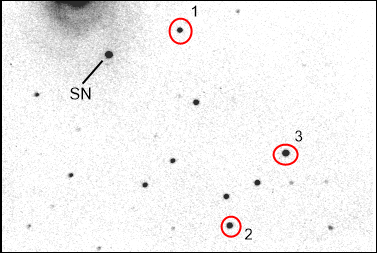
Figure 1: Supernova region of SN 2012aw. Circles indicate standard stars used for the photometry.

The light curves in four filters ($I$, $R$, $V$, $B$), obtained as a result of photometry, are shown in Figure 2. A comparison of the results of our photometry with data from the literature (Dall’Ora et al., 2014; Bose et al., 2013) is shown in Figure 3. The data are in quite good agreement with each other; our late time data complementing declining part of the light curves.

Table 2: Magnitudes of the standard stars marked in Figure 1.

Star	$\alpha_{J2000}$	$\delta_{J2000}$	B (mag)	V (mag)	R (mag)	I (mag)
1	$10^{h}43^{m}44^{s}.79$	$+11^{\circ}41^{\prime}03^{\prime\prime}.84$	15.351	14.972	14.706	14.450
2	$10^{h}43^{m}38^{s}.49$	$+11^{\circ}35^{\prime}02^{\prime\prime}.17$	15.551	14.669	14.145	13.670
3	$10^{h}43^{m}31^{s}.42$	$+11^{\circ}37^{\prime}16^{\prime\prime}.60$	14.992	13.932	13.248	12.717

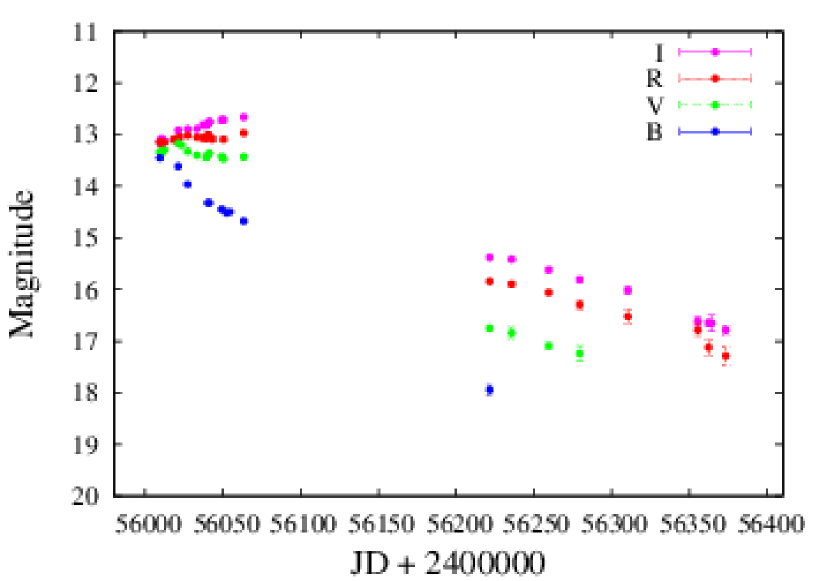
Figure 2: Light curve of SN 2012aw according to the results of our photometry. Observations performed on telescopes AZT-8 and LX200 (see Table 1). The Y axis shows the apparent magnitude.

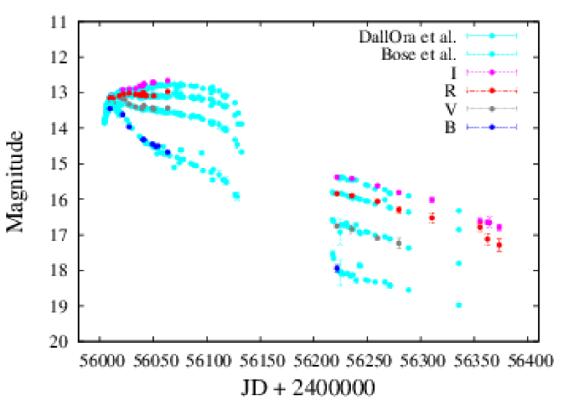
Figure 3: Comparison of the obtained light curve with photometric data from the literature (Dall’Ora et al., 2014; Bose et al., 2013). Blue dots indicate the results of photometry from the literature, other dots indicate the results of our photometry.

The Figure 4 shows a comparison of the light curve in $V$ band of supernova 2012aw with other SNe IIP: SN 1999em, SN 2004et, SN 2013ab, SN 2008in (Elmhamdi et al., 2003; Maguire et al., 2010; Bose et al., 2015; Roy et al., 2011). It can be seen that the studied supernova fits well into the general picture of the light curves of its type: there is a long region of the ”plateau”, followed by a sharp decline in brightness, which then goes on to the smooth and longest phase of the “tail”. Good agreement with other supernovae of that type can also be seen when comparing the SN 2012aw color indices with other SNe IIP (Figure 5).

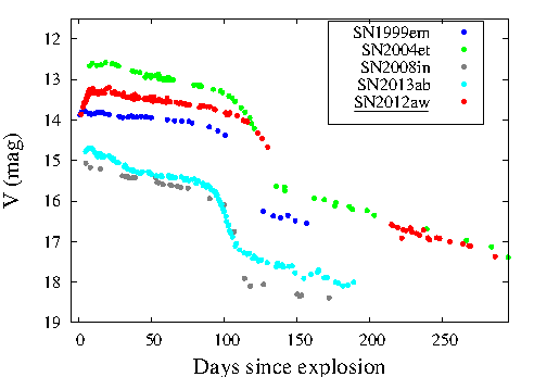
Figure 4: Comparison of the light curve of SN 2012aw with SNe IIP: SN 1999em, SN 2004et, SN 2013ab and SN 2008in. The Y axis represents the apparent magnitude in filter $V$.

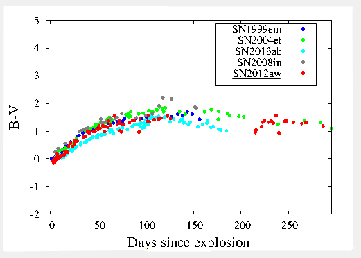
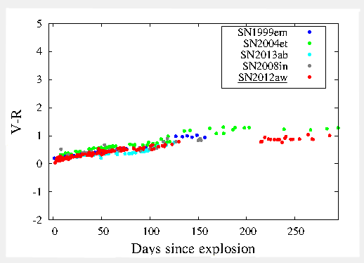
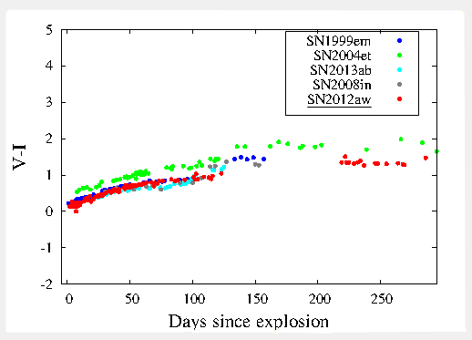
Figure 5: Comparison of color indices of SN 2012aw and other SNe IIP.

Table 3: Results of photometry of SN 2012aw obtained from AZT-8 and LX200 telescopes. The date $t_{0}$ is accepted as $JD=2456002.5$.

$JD+\footnotesize{2400000}$	Day	B(mag)	errB(mag)	V(mag)	errV(mag)	R(mag)	errR(mag)	I(mag)	errI(mag)	Telescope
56009.45	6.95	13.449	0.020	13.334	0.014	13.144	0.013	13.130	0.013	AZT-8
56010.48	7.98	-	-	13.332	0.026	13.156	0.017	13.078	0.017	AZT-8
56012.29	9.79	-	-	13.299	0.022	13.153	0.017	13.112	0.014	LX200
56018.41	15.91	-	-	-	-	13.096	0.021	-	-	LX200
56019.34	16.84	-	-	-	-	13.082	0.032	-	-	LX200
56021.35	18.85	13.611	0.044	13.166	0.038	-	-	12.911	0.032	AZT-8
56022.31	19.80	-	-	13.041	0.039	13.020	0.004	-	-	LX200
56023.38	20.84	-	-	13.201	0.031	-	-	-	-	LX200
56027.38	24.88	13.964	0.027	13.323	0.025	13.011	0.023	12.895	0.021	LX200
56033.30	30.80	-	-	13.398	0.021	13.048	0.018	12.887	0.028	LX200
56039.39	36.89	-	-	13.440	0.042	13.075	0.029	12.823	0.028	AZT-8
56040.39	36.90	-	-	-	-	13.014	0.023	12.782	0.024	LX200
56041.25	38.75	14.319	0.019	13.355	0.016	13.022	0.028	12.754	0.017	AZT-8
56043.320	40.82	-	-	-	-	13.087	0.038	-	-	LX200
56049.29	46.79	14.441	0.022	13.424	0.038	-	-	12.715	0.050	AZT-8
56050.41	47.91	-	-	13.465	0.025	13.089	0.031	12.713	0.032	LX200
56063.36	60.86	14.674	0.022	13.431	0.010	12.970	0.014	12.659	0.011	AZT-8
56221.61	219.11	17.941	0.098	16.748	0.058	15.843	0.020	15.376	0.040	AZT-8
56235.64	233.14	-	-	16.840	0.110	15.894	0.029	15.411	0.027	AZT-8
56259.59	257.09	-	-	17.093	0.053	16.058	0.032	15.620	0.036	AZT-8
56279.61	257.09	-	-	17.240	0.152	16.293	0.086	15.804	0.036	AZT-8
56310.54	308.039	-	-	-	-	16.520	0.133	16.015	0.064	LX200
56355.37	352.871	-	-	-	-	16.783	0.123	16.613	0.089	LX200
56362.39	359.891	-	-	-	-	17.119	0.160	16.648	0.058	LX200
56364.40	361.898	-	-	-	-	-	-	16.654	0.157	LX200
56373.45	370.949	-	-	-	-	17.284	0.170	16.786	0.093	LX200

2.2 Supernova Parameters from Observations

Photometry results for the SN 2012aw are presented in a number of works (Dall’Ora et al., 2014; Bose et al., 2013; Munari et al., 2013; Bayless et al., 2013). Bose et al. (2013) estimate the plateau duration $\approx 110$ days, Dall’Ora et al. (Dall’Ora et al., 2014) $\approx 100$ days.

We get an absolute magnitude in the middle of the plateau in the $V$ band equal to $-16.92$ mag, which is consistent with estimates from other works: $M_{v}=-16.67\pm 0.04$ mag (Bose et al., 2013). The luminosity peak at the early light curve of SN 2012aw in $U$, $B$, $V$, $R$, $I$ is reached at 8, 11, 15, 22, 24 days, respectively, thereby the supernova is similar to SN 1999em and SN 2004et (Bose et al., 2013).

The observed photospheric velocities for SN 2012aw ( $v=3.68(\times 10^{3})km/s$) were taken from Bose et al. (2013).

2.3 Estimation of observable parameters

We have estimated the observable parameters (the plateau duration $\Delta t$, the absolute magnitude $M_{V}$, and the photospheric velocity $u_{ph}$ at the middle of the plateau) from physical parameters (the explosion energy $E$, the mass of the envelope expelled $M$, and the pre-supernova radius $R$) using the relations found by Litvinova & Nadezhin (1985). Assuming $E=2.0$ foe, $M=25M_{\odot}$, $R=500R_{\odot}$ corresponding to our model R500M25Ni006E20 we obtained: $\Delta t=124$ days, $M_{V}=-17.5$, and $u_{ph}=4.26\times 10^{3}$ km s^-1. These results are not too different from the values described in the Section 2.2.

3 Hydrodynamic model

SNe IIP, like other type II supernovae, exhibit a wide variety of shapes of light curves. The shape of the light curve is mainly influenced by such parameters as the mass of the ejected supernova envelope $M$, the radius of the pre-supernova $R$, the explosion energy $E$ and the chemical composition of the star (Litvinova & Nadezhin, 1985).

We calculated a model which describes observational data of the SN 2012aw, using the multi-energy group radiation hydrodynamics code STELLA (Blinnikov et al., 2000, 1998). The advantage of the STELLA is that it can simultaneously calculate hydrodynamics and energy transfer. The non-stationary transport equation is solved assuming LTE simultaneously with the hydrodynamic equations. We calculated a grid of models in the parameter space $M$, $R$, ${}^{56}Ni$, $E$ to search for a model describing observational data for the 2012aw supernova.

For pre-SN we use a non-evolutionary polytropic model, like SN 1999em in the work of Baklanov et al. (2005). Figure 6 shows the density distribution and the mass fraction of chemical elements as a function of interior mass within the pre-supernova. It is assumed power-law dependence of the temperature on the density (Baklanov et al., 2005). In the center we isolate a dense core with the mass of 1.4 $M_{\odot}$, which collapses to a proto-neutron star. The explosion is initialized in STELLA as a thermal bomb just above the core mass.

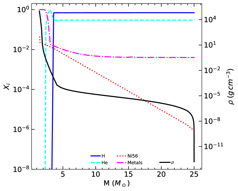
Figure 6: Distribution of chemical elements within the pre-supernova. The Y axis(right) displays the density, the Y axis(left) displays the relative content of the elements. Here ”Metals” means the fraction of all elements heavier than He.

The chemical composition of the host galaxy NGC 3351 is close to solar (Van Dyk et al., 2013; Fraser et al., 2012), therefore, for the outer layers of the pre-supernova shell, we adopt mass fractions of hydrogen $\mathrm{X}=0.735$, helium $\mathrm{Y}=0.248$, and the metallicity $\mathrm{Z}=0.17$.

The importance of joint fitting of light curves and expansion velocities of a supernova shell has been repeatedly emphasized in works with detailed modeling of supernovae (Blinnikov et al., 2000; Baklanov et al., 2005; Utrobin, 2007). This statement can be illustrated by fitting in two ways: first, the light curve only and, second, the light curve in combination with photospheric velocities.

In the first approach we come to the model R750M25Ni006E20 shown in Figure 7. This model, however, demonstrates a poor agreement between the observed and calculated photospheric velocities. It can be seen from the graph that the explosion energy in this model is not enough, and the shell scatters more slowly than was observed for SN 2012aw.

The observed photospheric velocities for SN 2012aw were taken from Bose et al. (2013). They were calculated from the absorption lines of Fe II in the late epochs and He I in the early epochs after the supernova explosion.

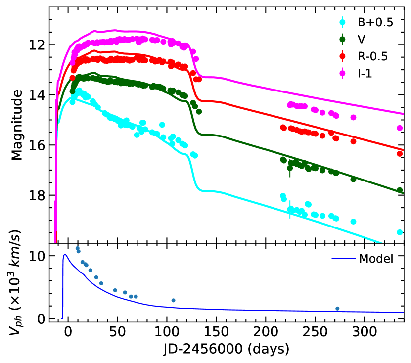
Figure 7: The model R750M25Ni006E20, accounting for photospheric velocities. Dots indicate observational data, four light curve lines indicate calculated curve, blue line below indicate calculated photospheric velocities. Light curves show good agreement between observations and modeling, but photospheric velocities from observations and modeling do not match.

We applied the fitting procedure, which takes into account both the light curves and the photospheric velocities of the supernova. We selected the R500M25Ni006E20 model, which provides a best fit to observational data of SN 2012aw (Figure 8) among other models.

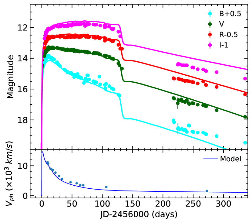
Figure 8: The best fit model when we are taking into account both light curves and photospheric velocities: R500M25Ni006E20

The pre-supernova radius in our model ($500R_{\odot}$) is comparable to the value of $430R_{\odot}$ reported by Dall’Ora et al. (2014). The mass of the ejected shell ($M_{ej}=23.6M_{\odot},M_{tot}=25M_{\odot}$) in our model is larger than that estimated by Dall’Ora et al. (2014) ($20M_{\odot}$). Our estimate of ⁵⁶Ni mass ($0.06M_{\odot}$) is consistent with values reported in previous works ($0.05-0.06M_{\odot}$). The mass of the ⁵⁶Ni in our model is also equal to $0.06M_{\odot}$. Previous estimates of SN 2012aw explosion energy — 1 foe (Bose et al., 2013), 1.5 foe (Dall’Ora et al., 2014), and 2 foe (Bose et al., 2014) — are close to our value of explosion energy (2 foe).

4 Discussion

A possible pre-supernova of the SN 2012aw was investigated by Van Dyk et al. (2013). They identified the object PTF12bvh as the progenitor of the SN 2012aw from archives of the Hubble Space Telescope, as well as from the ground-based observations in the near-infrared region. This field has been observed by the Hubble telescope at $F439W$, $F555W$ and $F814W$ between December 1994 and January 1995. Van Dyk et al. (2013) estimated the magnitude of the pre-supernova as $V=26.59$ mag.

Investigating the nature of the pre-supernova, Van Dyk et al. (2013) found that PTF12bvh is a red supergiant of class M3 with an effective temperature $T_{\rm eff}=$ 3600 K and a bolometric luminosity of $M_{\rm bol}=-8.29$ mag [$\log(L_{\rm bol}/L_{\odot})=5.21\pm 0.03$], effective radius $R_{\sim}1040\pm 100R_{\odot}$. The initial mass of the star was estimated as $\sim 17\div 18M_{\odot}$. Near the progenitor star, a significant amount of dust was noted.

The same object was identified as a pre-supernova in an earlier paper by Fraser et al. (2012). The bolometric luminosity was estimated as $\log(L/L_{\odot})=5.0\div 5.6$, according to a mass of $14-26M_{\odot}$. The temperature estimate range is $3300-4500$ K, which gives a radius of $R>500R_{\odot}$.

Estimates of pre-supernova parameters of the SN 2012aw differ in different studies. Our task is to put together all the previous results, to compare them with our results and to analyze them.

Estimates of the radius of the SN 2012aw pre-supernova star are as follows. Dall’Ora et al. (2014) obtained the radius of the progenitor $\sim 430R_{\odot}$ as a result of semi-analytical and hydrodynamic modelling. Based on analytical relations, Bose et al. (2013) obtained a not much different value $\sim 337\pm 67R_{\odot}$. A constraint on the radius of the pre-supernova star is also obtained from an analytical estimate $R>500R_{\odot}$ in (Fraser et al., 2012). According to Van Dyk et al. (2013), the pre-supernova had a radius $R=1040\pm 100R_{\odot}$. Martinez & Bersten (2019) derived $R=800\pm 100R_{\odot}$ from hydrodynamic modelling. We have got $R=500R_{\odot}$, which is close to the estimates found by Dall’Ora et al. (2014) and Fraser et al. (2012).

The initial mass of ⁵⁶Ni and the energy of the explosion do agree much better in the estimates of different studies: $M(^{56}$Ni$)\sim 0.06M_{\odot}$ (Dall’Ora et al., 2014), $M(^{56}$Ni$)\sim 0.06M_{\odot}$ (Hillier & Dessart, 2019), $M(^{56}$Ni$)$ $\sim 0.058\pm 0.002M_{\odot}$ (Bose et al., 2013), $M(^{56}$Ni$)$ $\sim 0.066\pm 0.006M_{\odot}$ (Martinez & Bersten, 2019). Our estimate of $M(^{56}$Ni$)\sim 0.06M_{\odot}$ is consistent with others.

Explosion energy from other studies: $E\sim 1.5\times 10^{51}$ erg (Dall’Ora et al., 2014), $E\sim 1\div 2\times 10^{51}$ erg (Bose et al., 2013), $E\sim 2\times 10^{51}$ erg (Bose et al., 2014), $E\sim 1.4\times 10^{51}$ erg (Martinez & Bersten, 2019), $E\sim 1.2\times 10^{51}$ erg (Hillier & Dessart, 2019). We have got the value $E={\color[rgb]{0,0,0}2.0}\times 10^{51}$ erg.

The initial mass of the star is estimated from $12.5\pm 1.5M_{\odot}$ (Fraser, 2016) to $21M_{\odot}$ (Dall’Ora et al., 2014). Van Dyk et al. (2013) estimated the initial mass of a star in the range of $15-20M_{\odot}$. Hillier & Dessart (2019) calculated the mass of progenitor as $15M_{\odot}$.

The most important result of our model is on the mass of the envelope ejected during the explosion. According to previous estimates we have rather high numbers for our object. Dall’Ora et al. (2014) rated the ejecta mass as $\sim 20M_{\odot}$. Bose et al. (2013) obtained a value of $14\pm 5M_{\odot}$ with large error estimate. Martinez & Bersten (2019) obtained $23_{-2}^{+1}M_{\odot}$. Our simulations with STELLA have the most detailed physics in comparison with all cited papers and they yield the best pre-supernova mass $23.6M_{\odot}$. The latter number is appreciably higher than the upper limit $17M_{\odot}$, which means the ‘Red Supergiant Problem’ problem persists (Smartt, 2009; Davies & Beasor, 2020; Kochanek, 2020). Moreover, recently there are more and more supernova models constructed for other objects with estimates of the ejecta mass appreciably larger than the Smartt’s limit: see, e.g. Utrobin & Chugai (2017), Utrobin & Chugai (2019). Thus, our results give one more confirmation that the theory of pre-supernova evolution is not yet fully understood, and this question deserves further investigation.

5 Conclusions

We report the results of our photometric observations of the SN 2012aw and compare it with the published data for this object.

To build our model we took into account both the light curves and the photospheric velocities of SN 2012aw. This is an important point that allows us to find the most suitable model among others.

We performed hydrodynamic modeling of both photometric and spectral data using the package STELLA and showed that the best agreement of the model with observations is found for the model R500M25Ni006E20. In this model the presupernova mass is $25M_{\odot}$ with the ejected $23.6M_{\odot}$, the explosion energy is 2.0 foe, the pre-supernova radius is $500R_{\odot}$, and the ⁵⁶Ni mass is $0.06M_{\odot}$. The total mass of SN 2012aw is higher by a factor of 1.5 compared with the upper Smartt’s limit, which emphasizes the RSG Problem.

Data availability

The photometric data are presented in Table  3. The details on calibrations are available from the first author upon request.

References

- Baklanov et al. (2005) Baklanov P. V., Blinnikov S. I., Pavlyuk N. N., 2005, Astronomy Letters, 31, 429
- Bayless et al. (2013) Bayless A. J., et al., 2013, ApJ, 764, L13
- Bersten et al. (2011) Bersten M. C., Benvenuto O., Hamuy M., 2011, ApJ, 729, 61
- Blinnikov et al. (1998) Blinnikov S. I., Eastman R., Bartunov O. S., Popolitov V. A., Woosley S. E., 1998, ApJ, 496, 454
- Blinnikov et al. (2000) Blinnikov S., Lundqvist P., Bartunov O., Nomoto K., Iwamoto K., 2000, ApJ, 532, 1132
- Bose et al. (2013) Bose S., et al., 2013, MNRAS, 433, 1871
- Bose et al. (2014) Bose S., Kumar B., Sutaria F., Roy R., Kumar B., Bhatt V. K., Chakraborti S., 2014, in Ray A., McCray R. A., eds, IAU Symposium Vol. 296, Supernova Environmental Impacts. pp 334–335, doi:10.1017/S1743921313009691
- Bose et al. (2015) Bose S., et al., 2015, MNRAS, 450, 2373
- Dall’Ora et al. (2014) Dall’Ora M., et al., 2014, ApJ, 787, 139
- Davies & Beasor (2020) Davies B., Beasor E. R., 2020, MNRAS, 493, 468
- Elmhamdi et al. (2003) Elmhamdi A., et al., 2003, MNRAS, 338, 939
- Fagotti et al. (2012) Fagotti P., et al., 2012, Central Bureau Electronic Telegrams, 3054, 1
- Fraser (2016) Fraser M., 2016, MNRAS, 456, L16
- Fraser et al. (2012) Fraser M., et al., 2012, ApJ, 759, L13
- Hamuy & Pinto (2002) Hamuy M., Pinto P. A., 2002, ApJ, 566, L63
- Hillier & Dessart (2019) Hillier D. J., Dessart L., 2019, A&A, 631, A8
- Kochanek (2020) Kochanek C. S., 2020, MNRAS, 493, 4945
- Litvinova & Nadezhin (1985) Litvinova I. Y., Nadezhin D. K., 1985, Soviet Astronomy Letters, 11, 145
- Maguire et al. (2010) Maguire K., et al., 2010, MNRAS, 404, 981
- Martinez & Bersten (2019) Martinez L., Bersten M. C., 2019, A&A, 629, A124
- Munari et al. (2013) Munari U., Henden A., Belligoli R., Castellani F., Cherini G., Righetti G. L., Vagnozzi A., 2013, New Astron., 20, 30
- Nomoto et al. (2006) Nomoto K., Tominaga N., Umeda H., Kobayashi C., Maeda K., 2006, Nuclear Phys. A, 777, 424
- Roy et al. (2011) Roy R., et al., 2011, ApJ, 736, 76
- Smartt (2009) Smartt S. J., 2009, ARA&A, 47, 63
- Smartt et al. (2009) Smartt S. J., Eldridge J. J., Crockett R. M., Maund J. R., 2009, MNRAS, 395, 1409
- Utrobin (2007) Utrobin V. P., 2007, A&A, 461, 233
- Utrobin & Chugai (2009) Utrobin V. P., Chugai N. N., 2009, A&A, 506, 829
- Utrobin & Chugai (2017) Utrobin V. P., Chugai N. N., 2017, MNRAS, 472, 5004
- Utrobin & Chugai (2019) Utrobin V. P., Chugai N. N., 2019, MNRAS, 490, 2042
- Van Dyk et al. (2013) Van Dyk S. D., Cenko S. B., Poznanski D., Arcavi I., Gal-Yam A., Filippenko A. V., et al. 2013, in American Astronomical Society Meeting Abstracts #221. p. 410.01