Abstract

Contemporary state-of-the-art approaches to Zero-Shot Learning (ZSL) train generative nets to synthesize examples conditioned on the provided metadata. Thereafter, classifiers are trained on these synthetic data in a supervised manner. In this work, we introduce Z2FSL, an end-to-end generative ZSL framework that uses such an approach as a backbone and feeds its synthesized output to a Few-Shot Learning (FSL) algorithm. The two modules are trained jointly. Z2FSL solves the ZSL problem with a FSL algorithm, reducing, in effect, ZSL to FSL. A wide class of algorithms can be integrated within our framework. Our experimental results show consistent improvement over several baselines. The proposed method, evaluated across standard benchmarks, shows state-of-the-art or competitive performance in ZSL and Generalized ZSL tasks.

1 Introduction

Deep Learning has seen great success in various settings and disciplines, like Computer Vision Krizhevsky et al. (2012); Zhou et al. (2017); Chen et al. (2019), Speech and Language Processing Devlin et al. (2019); Brown et al. (2020), Computer Graphics Starke et al. (2019); Park et al. (2019) and Medical Science Ronneberger et al. (2015); Rajpurkar et al. (2017). Despite the variety of applications, there is a common denominator: resources. The overwhelming majority of applications not only benefit from but necessitate voluminous data along with the associated hardware resources to achieve their reported results. This is evident both from their unprecedented, “superhuman” performance in many narrow tasks compared to traditional algorithms He et al. (2015); Silver et al. (2017) and their surprising deficiencies in low-data regimes. Consequently, resource requirements have skyrocketed. For instance, BERT’s Devlin et al. (2019) training requirements reach 256 TPU days.

A class of problems that deal with small and medium-sized data sets and distributions shifts are Zero-Shot Learning (ZSL) and Few-Shot Learning (FSL). These can prove interesting testing grounds for efficient learning. In these problems, and particularly in ZSL for Computer Vision tasks, Deep Learning has failed to have an immediate impact. It has only been applied in indirect ways, most notably by replacing image features extracted with traditional Computer Vision algorithms, like Bag of Visual Words Weston et al. (2010), with features extracted by deep nets such as ResNet He et al. (2016). Further integration of Deep Learning techniques is important to advance these settings.

A step towards that direction has been made with the inclusion of generative models. For FSL, various forms of autoencoders have been leveraged to provide additional, synthetic examples given the actual support set Antoniou et al. (2017); Wang et al. (2018); Xian et al. (2019). In ZSL, generative networks conditioned on some form of class descriptions are trained so as to generate synthetic samples of the test classes. In this way, the classification task is transformed into a standard supervised classification task. As a result, classifiers can be trained in a supervised manner Xian et al. (2018b); Zhu et al. (2018). More elaborate training techniques have been proposed Li et al. (2019b); Xian et al. (2019); Li et al. (2019a); Keshari et al. (2020); Narayan et al. (2020), yet without much progress on extending the basic approach.

In this work, we combine these two low-data regimes, namely ZSL and FSL. Specifically, we use the generative ZSL pipeline as a backbone and feed its synthesized output to a FSL classifier. The two modules can be trained jointly, rendering the overall process end-to-end. Formally, the FSL classifier’s loss is combined with the prior loss of the generative ZSL framework to form our proposed framework, Z2FSL. Z2FSL conceptually reduces ZSL to FSL by structuring the generator’s output as a support set for the FSL algorithm. Using the same FSL classifier during both training and testing is possible because of the flexibility of its output label space. This property holds because the FSL classifier can classify input patterns based on the examples and the classes present in its support set.

Our motivation and rationale for making the process end-to-end is threefold. First, the generative net gains access to the classification loss of the final classifier. This is beneficial because sample generation becomes more discriminative in a manner that explicitly helps the FSL classifier, since the latter’s loss drives the generation. Secondly, thanks to the aforementioned FSL property, the FSL classifier’s training is not reliant on the generated samples of the generator, so the former can be pre-trained on real examples. Additionally, this pre-training is not restricted to the corresponding training set of each task. For example, we can do so on ImageNet Deng et al. (2009). Lastly, Few-shot learners perform favorably compared to other alternatives in low-shot classification tasks Vinyals et al. (2016); Snell et al. (2017); Wang et al. (2018).

Our contributions to the study of ZSL are:

1. The coupling of two standard research benchmarks, ZSL and FSL, by our novel framework, Z2FSL, which makes generative ZSL approaches end-to-end by using a FSL classifier.

2. Formulating our framework in a manner that allows for a wide class of ZSL and FSL algorithms to be seamlessly integrated.

3. Achieving state-of-the-art or competitive performance on ZSL and Generalized ZSL benchmarks and analyzing the contributions of each component of our framework.

We have open-sourced our code.

2 Related Work

Earlier works address ZSL by splitting inference into two stages, inferring the attributes – the auxiliary description – of an image and then assigning the image to the closest given attribute vector. Examples are DAP Lampert et al. (2013) and the technique presented by Al-Halah et al. (2016). Alternatively, IAP Lampert et al. (2013) predicts the class posteriors and these are used to calculate the attribute posteriors of any image. Word2Vec Mikolov et al. (2013) descriptions have also been used instead of attributes, an example being CONSE Norouzi et al. (2013).

More recent research concentrates on learning a linear mapping from the image-feature space to a semantic space. ALE Akata et al. (2015a) learns a compatibility function between attributes and image features that is a bilinear form. SJE Akata et al. (2015b), DEVISE Frome et al. (2013), ESZSL Romera-Paredes & Torr (2015) and Qiao et al. (2016) learn a bilinear form as a compatibility function as well. SAE Kodirov et al. (2017) tackles ZSL with a linear autoencoder. Extending linear mappings, Xian et al. (2016) introduced LATEM, which is a piecewise-linear compatibility function.

Other recent approaches can be categorized as prototypical, because, at least conceptually, a prototype per class is computed. SYNC Changpinyo et al. (2016) align graphs in semantic and image-feature space, calculating prototypes in the process. CVCZSL Li et al. (2019b) learns a neural net that maps directly from attributes to image features, to class prototypes that is.

Currently, generative ZSL stands as the state of the art. The inaugural works of Xian et al. (2018b); Zhu et al. (2018) laid out the foundation, the basic generative approach, which can be broken down into three stages: first, a generative network is trained to generate instances of seen classes conditioned on the provided class descriptions. A differentiable classifier (e.g. pre-trained linear classifier, AC-GAN Odena et al. (2017)) can also be used to drive discriminative generation. In the second stage, given the description of every test class, the generative net is used to create a synthetic data set, transforming the problem into a supervised one. Then, a supervised classifier (SVM, linear, etc.) is trained on this data set. In the last stage, the classifier is tasked with classifying the actual test samples.

This basic approach has been somewhat enriched to improve performance. CIZSL Elhoseiny & Elfeki (2019) uses creative generation during training. LisGAN Li et al. (2019a) borrows from prototypical approaches and utilizes class representatives to anchor generation. f-VAEGAN Xian et al. (2019) shares weights between the decoder of a VAE and the generator of a WGAN to leverage the better aspects of both. GDAN Huang et al. (2019) uses cycle consistency. ZSML Verma et al. (2020) introduces meta-learning techniques. OCD Keshari et al. (2020) uses an over-complete distribution to generate hard examples and render the synthetic data set more informative. TF-VAEGAN Narayan et al. (2020) uses feedback to augment the f-VAEGAN.

In all cases, the proposed algorithms deviate from the basic approach mainly in the training regime of the generative net. In this paper, we describe Z2FSL, a generative ZSL framework which, via FSL, allows for improvements to the whole pipeline. In the next section, we describe in detail how this is achieved.

3 Preliminaries

In this section, we give all the necessary definitions, introduce notation and briefly discuss the necessary background.

3.1 Problem Definition

Let $\mathcal{X}_{tr}$ be the training samples and $\mathcal{X}_{ts}$ be the test samples. Let $\mathcal{Y}_{tr}$ be the corresponding set of training labels and $\mathcal{Y}_{ts}$ be the corresponding set of test labels.

In the ZSL setting, we have ${\mathcal{Y}_{tr}\cap\mathcal{Y}_{ts}=\emptyset}$, i.e. there are no common classes between training and testing, leading to the terms seen and unseen to describe the classes of the train and test setting respectively. In the Generalized ZSL (GZSL) setting, that restriction becomes ${\mathcal{Y}_{tr}\subset\mathcal{Y}_{ts}}$, meaning that there are samples from both unseen classes and every seen class during testing. Both in ZSL and GZSL, an auxiliary description of each class is provided to counterbalance the absence of training examples for unseen test classes. Such a description can be the Word2Vec representation of the class, an attribute vector or the Wikipedia article for the class.

In a FSL setting, it is sufficient to impose the restriction ${\mathcal{Y}_{tr}\subset\mathcal{Y}_{ts}}$, same as GZSL. However, no descriptions are provided. Rather, during testing, we are provided with a set of examples per test class, named support set. A support set essentially consists of labeled examples from all $n_{W}$ test classes, with $n_{S}$ examples each, where $n_{W}$ and $n_{S}$ are arbitrary natural numbers referred to as way and shot respectively. Also, let $S_{k}$ denote the set of examples of class $k$ in a support set. Given a support set, we are tasked with classifying a set of unlabeled samples of the same $n_{W}$ classes called query set. For convenience, we consider query sets to contain $n_{Q}$ samples per class, which is also an arbitrary natural number. Randomly sampling a support set and a corresponding query set from a (usually significantly) larger test data set constitutes an episode. The purpose of an episode is to test the ability of a model to generalize to possibly unseen classes given only a small number of examples of each class, seen or unseen, and its classification accuracy on the episode is naturally used as the metric of success. It is customary to report the average accuracy over many episodes to capture a more robust metric for a particular data set, where the way and the shot of the episodes remain constant. That is to say, a specific FSL setting is characterized by its way and shot and described as $n_{W}$-way $n_{S}$-shot, e.g. 25-way 4-shot refers to the regime where the support sets contain ${n_{W}=25}$ classes, with ${n_{S}=4}$ samples each.

3.2 Background

Wasserstein Generative Adversarial Net: Wasserstein Generative Neural Nets (WGAN) Arjovsky et al. (2017), an evolution of Generative Adversarial Nets Goodfellow et al. (2014), are a framework to train a generator $G$, formulating $p(x|z)$ of real samples $x$ with noise inputs $z$, in a minimax fashion with another network, a discriminator $D$. Gulrajani et al. (2017) added a regularization term to improve performance. We present the formulation of $p(x|a,z)$, which includes a conditioning variable $a$, namely

$$\begin{split}\mathcal{L}_{WGAN}&(G,D;p_{R},p_{Z})=\\ &\mathop{\mathbb{E}}_{(x,a)\sim p_{R},z\sim p_{Z}}\left[D(x,a)-D(G(a,z),a)\right]\\ &-\lambda\mathop{\mathbb{E}}_{(\hat{x},a)\sim p_{\hat{X}}}\left[(\|\nabla_{\hat{x}}D(\hat{x},a)\|_{2}-1)^{2}\right],\end{split}$$ (1)

where $p_{R}$ is the distribution of the real data, $p_{Z}$ a “noise” distribution, $p_{\hat{X}}$ the joint distribution of the conditioning variable and the uniform distribution on the line between $x$ and $G(a,z)$, $(x,a)\sim p_{R}$, $z\sim p_{Z}$ (intuitively $\hat{x}=ux+(1-u)G(a,z)$, $u\sim U(0,1)$) and $\lambda$ is a hyperparameter. The minimax game is defined as:

$$\begin{split}\min_{G}\max_{D}\mathcal{L}_{WGAN}(G,D;p_{R},p_{Z}).\end{split}$$ (2)

We use generator and generative net interchangeably.

Variational Autoencoder: The Variational Autoencoder (VAE), introduced by Kingma & Welling (2014), is an autoencoder that maximizes the variational lower bound of the marginal likelihood. An autoencoder consists of an encoder $E$, which compresses its input to a “latent” variable $z$, and a decoder $D$, which reconstructs the original input of $E$ based on $z$. We present the formulation of the VAE with a conditioning variable $a$,

$$\begin{split}\mathcal{L}_{VAE}&(E,D;p_{R},p_{\theta})=\\ &-\mathbb{E}_{(x,a)\sim p_{R}}[x\cdot\log{D(E(x,a),a)}\\ &\qquad+(1-x)\log{(1-D(E(x,a),a))}]\\ &+\mathbb{E}_{(x,a)\sim p_{R}}\left[D_{KL}(p_{E}(z|x,a)\|p_{\theta}(z))\right],\end{split}$$ (3)

where $D_{KL}$ is the Kullback-Leibler (KL) divergence, $p_{R}$ the distribution of the real data, $p_{E}$ the output distribution of $E$, which is a Gaussian Feedforward Neural Network (FFNN), i.e. it outputs the mean and the diagonal elements of the covariance of a Gaussian distribution, which makes the KL divergence analytical, and $p_{\theta}$ is the prior distribution of the “latent” variable. For practical purposes, the prior is set to $\mathcal{N}(.\ ;0,I)$, and the reparameterization trick Bengio et al. (2013) is used to sample from the encoder as ${z=\mu(x,a)+\epsilon\odot\sigma(x,a)}$, ${\epsilon\sim\mathcal{N}(\epsilon;0,I)}$, where $\odot$ is the Hadamard product and $\mu,\ \sigma$ the encoder’s outputs.

f-VAEGAN: f-VAEGAN Xian et al. (2019) is a generative ZSL approach that deploys both a WGAN and a VAE to train the generator, by sharing its weights between the VAE’s decoder and the WGAN’s generator. The overall loss function of the approach is

$$\begin{split}\mathcal{L}_{VAEGAN}&(G,E,D;p_{R},p_{Z},\beta)=\\ &\mathcal{L}_{VAE}(E,G;p_{R},p_{Z})\\ &+\beta\cdot\mathcal{L}_{WGAN}(G,D;p_{R},p_{Z}),\end{split}$$ (4)

where $E$ is the encoder of the VAE, $D$ the discriminator of the WGAN, $G$ the generator of the WGAN and the decoder of the VAE and $\beta$ a hyperparameter.

Prototypical Network: Prototypical Networks (PN) Snell et al. (2017) present a simple, differentiable framework for FSL. A neural network, $f_{\phi}$, is used to map the input samples to a metric space. The support set is mapped and the embeddings are averaged per class so as to get a prototype $c_{k}$ for each. Then, each sample in the query set is mapped to the metric space and classified to the nearest prototype based on the Euclidean distance $d(\cdot\ ,\cdot)$. The formulation is

$$\begin{split}c_{k}=\ &\frac{1}{|S_{k}|}\sum_{x_{i}\in S_{k}}f_{\phi}(x_{i}),\\ p_{\phi}(y=k|x)=\ &\frac{\exp{(-d(f_{\phi}(x),c_{k}))}}{\sum_{k^{\prime}}\exp{(-d(f_{\phi}(x),c_{k^{\prime}}))}},\\ \mathcal{L}_{PN}(f_{\phi};S,Q)=\ &\frac{1}{|Q|}\sum_{(x_{i},y_{i})\in Q}\log{p_{\phi}(y=y_{i}|x)},\\ \end{split}$$ (5)

where $p_{\phi}(y|x)$ is the softmax output distribution of $x$ belonging to some class. To compute $\mathcal{L}_{PN}$, we have to sample episodes instead of batches. In this manner, training resembles testing. We refer to that manner of training as episodic.

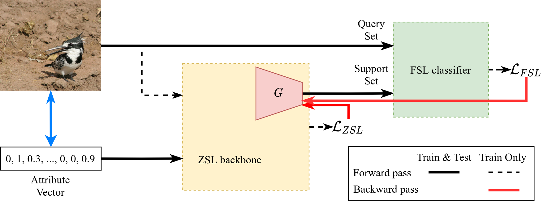
Figure 1: Graphical representation of the Z2FSL framework and pipeline. We use a generative Zero-shot Learning backbone with a Few-shot Learning classifier. During training, we train the generator $G$ with a combination of its training within the backbone and the Few-shot Learning classification task. During testing, the forward pass is only altered in that real examples are not provided to the backbone and no backward pass is performed.

4 Method

We now describe the proposed Z2FSL framework in detail. In Z2FSL, a generative ZSL pipeline, used as a backbone, is coupled with a FSL classifier. We can train the two modules jointly by conceptually reducing ZSL to FSL, which simply means that the backbone generates the classifier’s support set. To get an episode, real examples of the classes that are present in this support set can be used as the query set. During testing, the test samples become the query and the support is again provided by the backbone. The framework is also presented in Figure 1, where a graphical representation of how the novel component of our framework, the FSL classifier, affects the pipeline can be seen. The backbone provides the support set of the FSL classifier in all settings. During training, this allows the back-propagation of the FSL loss to the generator. During testing, synthesized examples of the test classes are provided in order to enable the classification of unseen classes.

This is possible because the FSL algorithm can classify its input dynamically, in the sense that its output distribution is based on the classes present in the support set. This allows us to train the classifier on classes other than the unseen classes and simply provide the necessary synthetic support set during testing. Another advantage is that the FSL algorithm can actually be pre-trained before the joint training with the backbone and/or fine-tuned afterwards, or even trained completely separately of the backbone.

4.1 Training

We train all the components for multiple iterations. As an example, the components in this work, other than the generator and the FSL classifier, which are also visible in Figure 1, include the discriminator of a WGAN and the encoder of a VAE. In each iteration, we take steps training the components: training the FSL classifier, training the generator and training all the other components as necessary.

First, when training the FSL algorithm, we randomly sample query sets from the training set and support sets are generated by the backbone, conditioned on the metadata of the classes that appear in the query set. The FSL loss, denoted $\mathcal{L}_{FSL}$, remains intact (e.g. Equation 5 for PNs). This is a slightly modified version of the episodic training we defined in Section 3.1, since the support set is now synthetic. Episodes during training, $n_{W}$, $n_{S}$ and $n_{Q}$ in particular, can be set arbitrarily, similar to batches. The process can be seen indirectly in Figure 1. For this step, we would have to simply back-propagate $\mathcal{L}_{FSL}$ only to the FSL classifier.

Second, when training the generator of the ZSL backbone, we use the loss within the generative framework of the backbone, which we denote as $\mathcal{L}_{ZSL}$ (e.g. Equation 4 if the backbone is the f-VAEGAN). By feeding the generated samples to the FSL algorithm, we can back-propagate $\mathcal{L}_{FSL}$ to the generator. This also requires sampling a query set based on the classes the generator provides. The overall objective of the ZSL generator is then described as:

$$\mathcal{L}_{Z2FSL}=\mathcal{L}_{ZSL}+\gamma\mathcal{L}_{FSL},$$ (6)

where $\gamma$ is a hyperparameter. This is the step depicted in Figure 1 if we take into account all arrows.

The rest of the components can be trained before or after the two aforementioned steps. In this work, for example, we update the discriminator multiple times before each generator update, as suggested by Goodfellow et al. (2014); Arjovsky et al. (2017).

However, components of the backbone can even be trained along with the generator. A component that does not affect the generation of the support set in the forward pass can be trained along with the generator, but it remains unaffected by $\mathcal{L}_{FSL}$. Such a component is the encoder of a VAE, which we also use in our work, or a regressor for cycle consistency Huang et al. (2019). A component that affects generation in the forward pass, such as a feedback module Narayan et al. (2020), can be trained along with the generator and updated based on the objective in Equation 6 rather than $\mathcal{L}_{ZSL}$ alone.

In Figure 1, we can more generally see that both real examples and corresponding descriptions are provided to the backbone, while only real and generated examples to the classifier. Real samples are useful to the backbone only during training, e.g. to compute the VAE reconstruction loss.

4.2 Evaluation

For the evaluation, the pipeline is modified in two ways. First, as shown in Figure 1, we stop providing real samples to the backbone. Only the descriptions are necessary so as to generate the test support set. Second, episodes are restricted by the test setting. The number of classes in each set, $n_{W}$, is fixed and equal to the number of test classes. $n_{Q}$ is equal, for each test class, to the number of test samples available. $n_{S}$ remains a hyperparameter, as we can choose the number of samples to generate per class. In this manner, the query set contains all test samples and the FSL classification accuracy is exactly the final ZSL accuracy.

4.3 Assumptions

We make three assumptions about the backbone and the classifier altogether. First, the backbone is a generative ZSL approach. Second, the classifier is trained through a differentiable process. Third, the classifier can classify its input dynamically, by matching support and query classes Vinyals et al. (2016); Snell et al. (2017); Wang et al. (2018). This fact allows the usage of the classifier during testing without any training on unseen classes as long as corresponding supporting examples are provided at that time. This means that the classifier is not reliant on the generator and, consequently, the modules can be trained separately or jointly.

As a result, our framework is suitable for a wide class of ZSL and FSL algorithms. We formulate our framework as agnostic to the generative ZSL and the FSL algorithm, and refer to a specific implementation of it by the following macro: Z2FSL(z, f), where z is the generative ZSL backbone and f the FSL classifier.

5 Experiments

We first present the datasets, followed by implementation details and finally present our experimental results along with comparison to state ot the art.

5.1 Data sets

We use the Caltech UCSD Bird 200 (CUB, Wah et al. 2011), which consists of 11788 images of birds belonging to 200 species. One 312-dimensional attribute vector per class is provided as well. We also use Animals with Attributes 2 (AwA2, Xian et al. 2018a). It contains 37322 images from 50 categories and 85-dimensional attributes. Our last data set is the SUN Scene Classification (SUN, Patterson & Hays 2012) data set, with 14340 images of 717 categories and 102-dimensional attributes.

We use the provided attributes as our auxiliary descriptions, and in particular the continuous attributes after normalizing them w.r.t. their L2 norm. We use 10 crops per image (original image, top-right, top-left, bottom-right, bottom-left and their horizontally flipped counterparts) as augmentation. We use the original image for testing. Instead of images, we use features extracted by the ResNet-101 He et al. (2016) trained on ImageNet Deng et al. (2009). We choose the 2048-dimensional output of its adaptive average pooling layer. Additionally, we perform min-max normalization of the features to $[0,1]$ and use the train-test and seen-unseen splits proposed by Xian et al. (2018a).

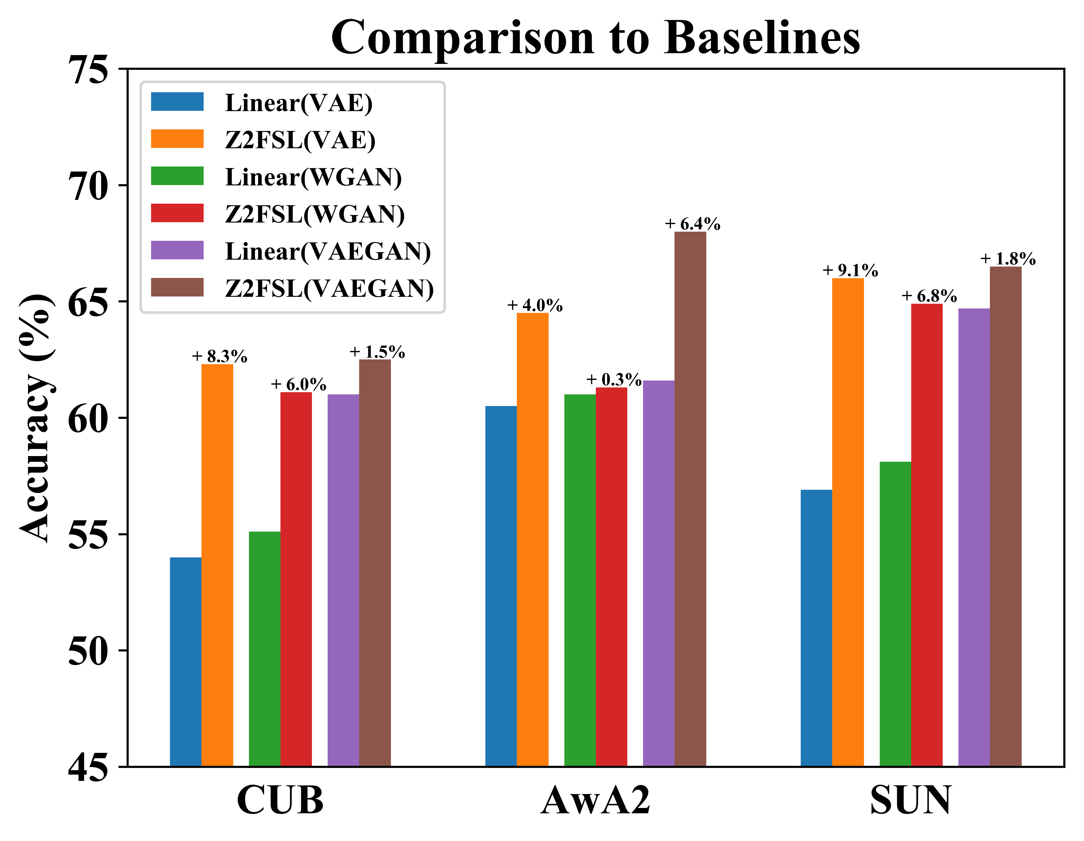
Figure 2: Comparison of Z2FSL to baseline generative ZSL backbones. Linear(z) describes the setting where the generative ZSL approach z is used with a linear classifier trained on the generated data. We skip the second argument of the Z2FSL macro for convenience, since it is the PN in all cases. Linear(VAEGAN) results for CUB and SUN reported from Xian et al. (2019). The metric presented is the average per class top-1 accuracy. Performance gains denote absolute improvement compared to the corresponding baseline.

5.2 Implementation Details

Since we present the results of Z2FSL(f-VAEGAN, PN) in comparison to the state of the art, we present details for that specific architecture in this section.

We pre-train the PN in an episodic manner as suggested by Snell et al. (2017), where support and query sets are sampled from the real training data of the corresponding data set. The PN is implemented as a FFNN with $n_{h}$ hidden layers with square weight matrices and ReLU activations. The FSL classifier’s learning rate is kept the same in pre-training and the joint training with the generator.

The generator and the encoder are FFNNs with 2 hidden layers each, 4096 followed by 8192 units for the generator and the reverse for the encoder, Leaky ReLU hidden activations (0.2 slope), linear output for the encoder and sigmoid for the generator. The noise dimension is chosen to be equal to the dimension of the attributes. The discriminator is a FFNN with one hidden layer of 4096 neurons and Leaky ReLU hidden activations (0.2 slope). We set the coefficient of the regularization term of WGAN $\lambda=10$ and the training updates of the discriminator per generator update equal to 5.

When we sample support sets from the generative net, we set $n_{S}=5$ during training. During testing, we set it to $n_{S}=1800$ for unseen classes. For seen classes in the GZSL test setting, we experiment with both seen and unseen support and select the better alternative for each benchmark. We also consider the shot of the test support set for seen classes a different hyperparameter $m_{S}$.

The optimizer in all cases is Adam Kingma & Ba (2015) with $\beta_{1}=0.5$ and $\beta_{2}=0.999$. We apply gradient clipping, restricting the gradient for each parameter within $[-5,5]$. Our implementation is in PyTorch Paszke et al. (2019).

The tunable hyperparameters that we either search for or vary by data set are presented in the Supplementary Material.

Table 1: Comparison of our approach, Z2FSL(f-VAEGAN, PN), to previous work. The metric presented is the average per class top-1 accuracy.

	Zero-shot Learning
Approach	CUB	AwA2	SUN
CVCZSL Li et al. (2019b)	54.4	71.1	62.6
f-CLSWGAN Xian et al. (2018b)	57.3	-	60.8
LisGAN Li et al. (2019a)	58.8	-	61.7
f-VAEGAN Xian et al. (2019)	61.0	-	64.7
OCD Keshari et al. (2020)	60.3	71.3	63.5
TF-VAEGAN Narayan et al. (2020)	64.9	72.2	66.0
Z2FSL(f-VAEGAN, PN)	62.5	68.0	66.5

5.3 Backbone Baselines

In this section, we present the performance of our framework using various generative ZSL approaches as backbones and compare that with the plain generative ZSL approaches, i.e. without the FSL algorithm, as baselines. The comparison can be seen in Figure 2. The baselines we have chosen are a VAE, a WGAN and a f-VAEGAN. Z2FSL improves the performance of all baselines consistently across all benchmarks. It is interesting to see that, in most cases, the simple backbones, the VAE and the WGAN, enhanced by our framework, exceed the performance of the more elaborate and superior – on its own – plain f-VAEGAN.

5.4 State of the art

In this section, we present our results in comparison with the current state-of-the-art approaches that use the same test setting as our approach (feature extractor, dimensionality of features, splits, etc. described in Sections 5.1 and 5.2).

Table 2: Comparison of our approach, Z2FSL(f-VAEGAN, PN), to previous work. The metrics presented are: $\mathbf{u}$ is the average per class top-1 accuracy of unseen classes, $\mathbf{s}$ is the average per class top-1 accuracy of seen class and $\mathbf{H}$ their harmonic mean. $\mathbf{H}$ is considered the main metric of this setting.

	Generalized Zero-shot Learning
	CUB			AwA2			SUN
Approach	u	s	H	u	s	H	u	s	H
CVCZSL Li et al. (2019b)	47.4	47.6	47.5	56.4	81.4	66.7	36.3	42.8	39.3
f-CLSWGAN Xian et al. (2018b)	43.7	57.7	49.7	-	-	-	42.6	36.6	39.4
LisGAN Li et al. (2019a)	46.5	57.9	51.6	-	-	-	42.9	37.8	40.2
f-VAEGAN Xian et al. (2019)	48.4	60.1	53.6	-	-	-	45.1	38.0	41.3
OCD Keshari et al. (2020)	44.8	59.9	51.3	59.5	73.4	65.7	44.8	42.9	43.8
TF-VAEGAN Narayan et al. (2020)	52.8	64.7	58.1	59.8	75.1	66.6	45.6	40.7	43.0
Z2FSL(f-VAEGAN, PN)	47.2	61.2	53.3	57.4	80.0	66.8	44.0	32.9	37.6

5.4.1 Zero-shot Learning

For ZSL, our experimental evaluation in Section 5.3 shows that Z2FSL(f-VAEGAN, PN) outperforms the f-VAEGAN. This performance compares favorably to the rest of the state-of-the-art approaches as well, as can be seen in Table 1. In particular, even though the TF-VAEGAN itself builds on top of the f-VAEGAN and improves performance, our approach outperforms that on SUN, where it achieves state-of-the-art performance, improving the previous one by an absolute margin of $0.5\%$.

5.4.2 Generalized Zero-shot Learning

For GZSL, results can be seen in Table 2. Performance in AwA2 is marginally better than the previous state of the art, CVCZSL and TF-VAEGAN. In contrast, in CUB and SUN it is harder to balance seen and unseen accuracies, as decreasing the $s$ metric, which is partly controlled by $m_{S}$, is required to achieve the best $H$ possible. This leads to inferior performance compared to our specific backbone in SUN and marginally worse accuracy in CUB. The state-of-the-art results in AwA2 can be partly explained by the small number of classes, which are 50 in total, only 10 of which are unseen.

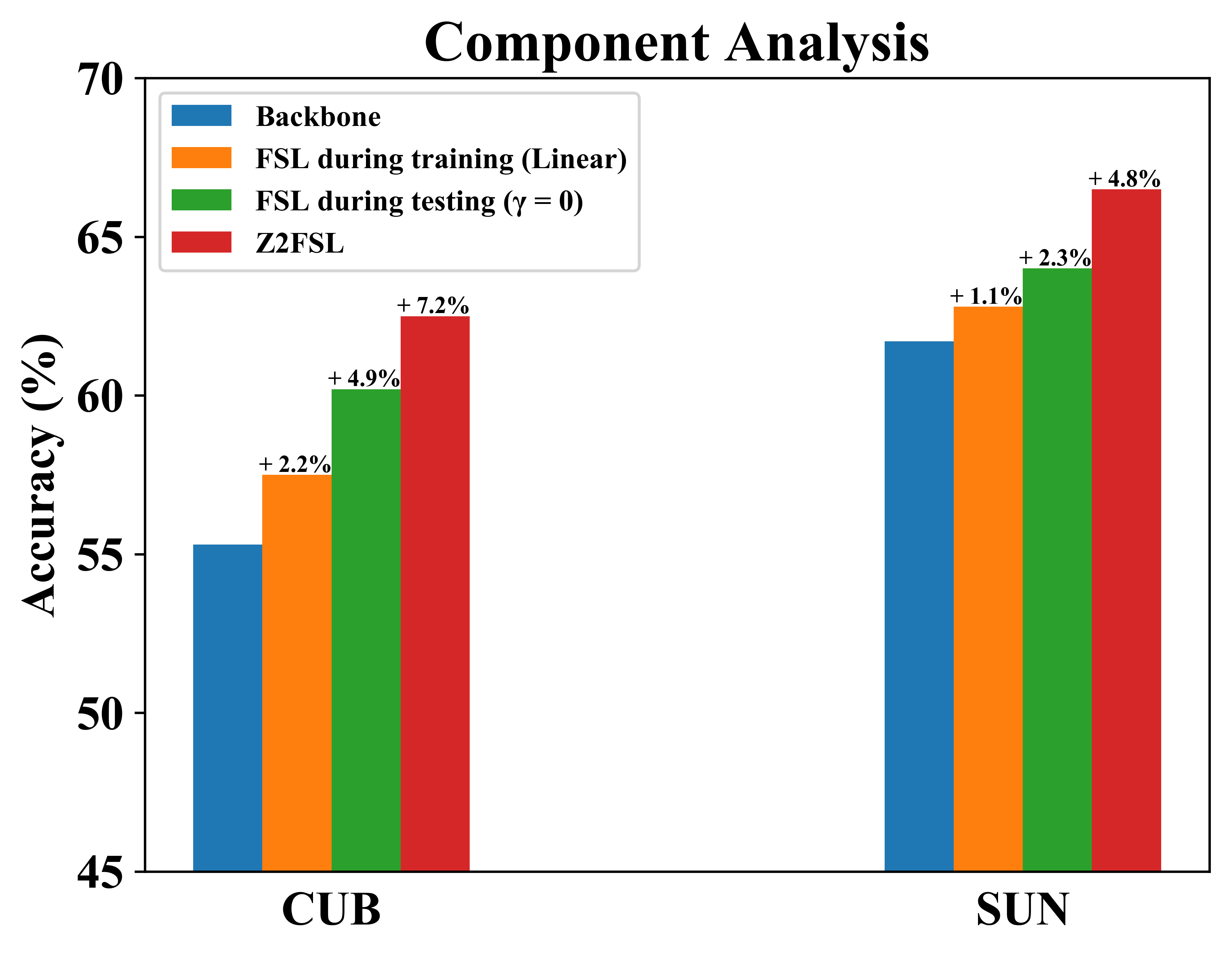
Figure 3: FSL classifier’s effects on performance. We compare the performance of the f-VAEGAN, the backbone generative ZSL approach, to the performance of Z2FSL(f-VAEGAN, PN) when we discard the FSL classifier during the evaluation and use a linear classifier instead, the performance of Z2FSL(f-VAEGAN, PN) when $\gamma=0$ (Equation 6), i.e. discarding the FSL classifier during training only, and the complete Z2FSL(f-VAEGAN, PN) (with the FSL classifier in both settings). The metric presented is the average per class top-1 accuracy. Performance gains denote absolute improvement compared to the backbone.

Table 3: Comparison of our approach, Z2FSL(f-VAEGAN, PN) with real and synthetic support for seen classes. The metrics presented are: $\mathbf{u}$ is the average per class top-1 accuracy of unseen classes, $\mathbf{s}$ is the average per class top-1 accuracy of seen class and $\mathbf{H}$ their harmonic mean.

	Generalized Zero-shot Learning
	CUB			AwA2			SUN
Approach	u	s	H	u	s	H	u	s	H
Z2FSL(f-VAEGAN, PN) (with real support)	47.2	61.2	53.3	49.4	77.7	60.4	48.1	27.4	34.9
Z2FSL(f-VAEGAN, PN)	44.4	58.0	50.3	57.4	80.0	66.8	44.0	32.9	37.6

5.5 Ablation studies

5.5.1 Component Analysis

We perform a more detailed analysis of how the usage of the novel component of our approach, the FSL classifier, affects performance. We experiment with using the FSL classifier solely during the training of the backbone. During testing, we follow the standard practise of training a linear classifier on the synthetic data. We also experiment with using the FSL classifier only during testing, i.e. simply setting $\gamma=0$ in Equation 6. Results are presented in Figure 3. We can observe that both regimes yield improvement compared to the plain backbone. Additionally, regarding the gains in performance compared to the backbone, the gain of Z2FSL is greater than the sum of the gains of the two ablation studies. This shows that end-to-end training yields a significant improvement and validates that this process renders the generation discriminative in a manner that explicitly helps the classifier.

Table 4: Comparison of our approach, Z2FSL(f-VAEGAN, PN), with and without pre-training the FSL classifier. The metric presented is the average per class top-1 accuracy.

	ZSL
Approach	CUB	SUN
Z2FSL (no pre-training)	58.0	61.3
Z2FSL	62.5	66.5

5.5.2 Synthetic vs. Real Support Set

We also examine the performance of Z2FSL when using real supporting examples of seen classes compared to performance with synthetic ones. Results are presented in Table 3. In AwA2 and SUN, the synthetic support results in a better harmonic mean. On the other hand, in CUB, real support leads to an increase in performance. Moreover, as we noted in Section 5.2, the shot for seen classes in the test support set is controlled by a different hyperparameter than that of unseen classes, $m_{S}$ and $n_{S}$ (for testing) respectively . These facts clearly demonstrate the bias towards seen classes the naive approaches of using all the available training data in the support set or too many synthetic ones could lead to.

5.5.3 Pre-training

We also test the effects of pre-training the FSL classifier of our framework. It makes sense, intuitively, to pre-train it in an actual FSL setting before the joint training with the generator, where we choose to train it with a combination of real and synthetic data. Table 4 shows a decrease in performance without pre-training, 5.2% absolute decrease in SUN and 4.5% in CUB to be exact. This illustrates that training in the FSL setting is essential to avoid overfitting.

6 Conclusions

In this paper, we introduce a novel, end-to-end generative ZSL framework, Z2FSL. Z2FSL uses the same supervised classifier during both training and testing. We choose a FSL algorithm to fill that role, since the choice of classifier is restricted by the ZSL setting. In this manner, we also couple the two low-data regimes. We formulate our framework so as to allow a broad class of generative ZSL approaches and FSL classifiers to be integrated. Empirically, we show that our framework improves upon the results of the plain generative approach. Extensive ablation studies reveal that the improvement originates from the fact that the generated samples of the generative net are rendered more discriminative in a way that explicitly helps the classifier. In addition, these studies demonstrate the advantages of being able to use a pre-trained classifier. Our results are state of the art or competitive across all benchmarks. We also show that using synthetic samples for seen classes as well as decreasing the number of samples of these classes compared to unseen ones can improve performance in GZSL.

Our future plans include further investigating and mitigating the bias towards seen classes in the GZSL. Another research direction we plan to investigate are techniques to better train the FSL classifier separately of the generator. Initial thoughts include consistent fine-tuning on generated samples of unseen classes after the joint training and extensive pre-training on other data sets. Since we now have an end-to-end process to train the generative net, it is possible to completely dispose of the generative framework and, therefore, we also plan to investigate this training regime.

Table 5: Hyperparameter configuration per setting and data set for the Prototypical Network’s pre-training. From top to bottom, the hyperparameters presented are the learning rate of the FSL algorithm $\alpha_{h}$, the number of episodes $N_{h}$, the number of hidden layers $n_{h}$, the number of classes in an episode $n_{W}$, the number of support examples per class $n_{S}$, and the number of queries per class $n_{Q}$.

	ZSL			GZSL
Hyperparameter	CUB	AwA2	SUN	CUB	AwA2	SUN
$\alpha_{h}$	$5\cdot 10^{-5}$	$10^{-5}$	$10^{-5}$	$10^{-3}$	$10^{-5}$	$5\cdot 10^{-5}$
$N_{h}$	12000	15000	10000	10000	12000	8000
$n_{h}$	0	1	1	0	1	1
$n_{W}$	25	10	40	25	10	50
$n_{S}$	5	5	5	5	5	5
$n_{Q}$	10	15	5	10	15	2

Table 6: Hyperparameter configuration per setting and data set for our main experiments. We have the ZSL learning rate $\alpha_{f}$, the coefficient of the WGAN loss $\beta$, the coefficient of the FSL loss $\gamma$, the number of classes in a training episode $n_{W}$, the number of generations per class in during training $n_{S}$, the number of generations per seen class during testing $m_{S}$, the number of “queries” per class in a training episode $n_{Q}$, and the number of episodes $N$.

	ZSL			GZSL
Hyperparameter	CUB	AwA2	SUN	CUB	AwA2	SUN
$\alpha_{f}$	$10^{-4}$	$10^{-4}$	$10^{-4}$	$10^{-4}$	$10^{-4}$	$10^{-4}$
$\beta$	100	100	100	100	100	100
$\gamma$	100	100	100	10	10	10
$n_{W}$	25	10	80	25	10	80
$n_{S}$	5	5	5	5	5	5
$m_{S}$	-	-	-	5	2	5
$n_{Q}$	10	15	5	10	15	5
$N$	8000	8000	6500	6500	8500	8000

Appendix A Evaluation Metrics

For the sake of completeness, we formally define the the Zero-Shot Learning (ZSL) and Generalized Zero-Shot Learning (GZSL) metrics we use. We evaluate our framework with the average per-class [top-1] accuracy for ZSL, defined as

$$\begin{split}acc_{\mathcal{Y}}=\frac{1}{\|\mathcal{Y}\|}\sum_{y\in\mathcal{Y}}\frac{\text{\# correct predictions in y}}{\text{\# samples in y}},\end{split}$$ (7)

where in the case of ZSL $\mathcal{Y}$ are the unseen classes. For GZSL, we use the harmonic mean of the average per-class accuracy of seen classes and that of unseen classes, defined as

$$\begin{split}H=2\frac{u\cdot s}{u+s},\end{split}$$ (8)

where we define $u=acc_{\mathcal{Y}}$ for unseen classes and $s=acc_{\mathcal{Y}}$ for seen classes for convenience and adherence to established notation.

Appendix B Hyperparameters

We present the rest of the hyperparameters for the pre-training of the Few-Shot Learning (FSL) algorithm, the Prototypical Network (PN), in Table 5 and for the training within our framework, Z2FSL(f-VAEGAN, PN), in Table 6, both for Zero-Shot Learning (ZSL) and Generalized Zero-shot Learning (GZSL).

Appendix C Classifier Fine-tuning

After the joint training of the FSL classifier and the generator of the backbone, we fine-tune the FSL classifier on samples generated by the generator conditioned on attributes of the unseen classes. This basically means that the generator provides both the support and the query set. We train for 25 episodes, using the same learning rate as in the other two settings the classifier is trained. We also retain the hyperparameters of the episode in this training regime the same as in the joint training of the FSL classifier and the generator. This process provides marginal improvement, if any, and is generally inconsistent. Further work is required to stabilize it.

Appendix D Prototypical Network initialization

We initialize the weight matrices of the PN by setting all the diagonal elements equal to 1, while the rest are randomly sampled i.i.d. from $\mathcal{N}(.\ ;0,0.01)$. We do so to bias the PN to preserve its input space structure as much as possible, which we expect to be somewhat discriminative due to ResNet-101. Notice that we can do so because ResNet-101 yields non-negative values and we use ReLU activations. This structure can be thought of as similar to a residual layer He et al. (2016) routinely used in Convolutional Neural nets. It is for this reason that all weight matrices in the PN are square. We observed an increase in validation accuracy in all settings using this clever initialization trick. We are unaware of another similar approach in the literature, so further investigation may be warranted.

Appendix E Data Augmentation

For the extra crops besides the original image, we crop the original image starting from the desired corner and extending up to 80% of each dimension and finally resize the crop to match the original image’s dimensions.

References

- Akata et al. (2015a) Akata, Z., Perronnin, F., Harchaoui, Z., and Schmid, C. Label-embedding for image classification. IEEE Trans. Pattern Anal. Mach. Intell., 38(7):1425–1438, 2015a.
- Akata et al. (2015b) Akata, Z., Reed, S., Walter, D., Lee, H., and Schiele, B. Evaluation of output embeddings for fine-grained image classification. In IEEE Conf. Comput. Vis. Pattern Recog., pp. 2927–2936, 2015b.
- Al-Halah et al. (2016) Al-Halah, Z., Tapaswi, M., and Stiefelhagen, R. Recovering the missing link: Predicting class-attribute associations for unsupervised zero-shot learning. In IEEE Conf. Comput. Vis. Pattern Recog., pp. 5975–5984, 2016.
- Antoniou et al. (2017) Antoniou, A., Storkey, A., and Edwards, H. Data Augmentation Generative Adversarial Networks. arXiv preprint arXiv:1711.04340, 2017.
- Arjovsky et al. (2017) Arjovsky, M., Chintala, S., and Bottou, L. Wasserstein gan. In Int. Conf. Mach. Learn., pp. 214–223, 2017.
- Bengio et al. (2013) Bengio, Y., Léonard, N., and Courville, A. Estimating or propagating gradients through stochastic neurons for conditional computation. arXiv preprint arXiv:1308.3432, 2013.
- Brown et al. (2020) Brown, T. B., Mann, B., Ryder, N., Subbiah, M., Kaplan, J., Dhariwal, P., Neelakantan, A., Shyam, P., Sastry, G., Askell, A., et al. Language models are Few-shot Learners. arXiv preprint arXiv:2005.14165, 2020.
- Changpinyo et al. (2016) Changpinyo, S., Chao, W.-L., Gong, B., and Sha, F. Synthesized Classifiers for Zero-shot Learning. In IEEE Conf. Comput. Vis. Pattern Recog., pp. 5327–5336, 2016.
- Chen et al. (2019) Chen, W., Ling, H., Gao, J., Smith, E., Lehtinen, J., Jacobson, A., and Fidler, S. Learning to predict 3d objects with an interpolation-based differentiable renderer. In Adv. Neural Inform. Process. Syst., pp. 9609–9619, 2019.
- Deng et al. (2009) Deng, J., Dong, W., Socher, R., Li, L.-J., Li, K., and Fei-Fei, L. ImageNet: A large-scale hierarchical image database. In IEEE Conf. Comput. Vis. Pattern Recog., pp. 248–255, 2009.
- Devlin et al. (2019) Devlin, J., Chang, M.-W., Lee, K., and Toutanova, K. BERT: Pre-training of deep bidirectional transformers for language understanding. In Proceedings of the Conference of the North American Chapter of the Association for Computational Linguistics: Human Language Technologies, volume 1, pp. 4171–4186. Association for Computational Linguistics, 2019.
- Elhoseiny & Elfeki (2019) Elhoseiny, M. and Elfeki, M. Creativity inspired Zero-shot Learning. In Int. Conf. Comput. Vis., pp. 5784–5793, 2019.
- Frome et al. (2013) Frome, A., Corrado, G. S., Shlens, J., Bengio, S., Dean, J., Ranzato, M., and Mikolov, T. Devise: A deep visual-semantic embedding model. In Adv. Neural Inform. Process. Syst., pp. 2121–2129, 2013.
- Goodfellow et al. (2014) Goodfellow, I., Pouget-Abadie, J., Mirza, M., Xu, B., Warde-Farley, D., Ozair, S., Courville, A., and Bengio, Y. Generative adversarial nets. In Adv. Neural Inform. Process. Syst., pp. 2672–2680, 2014.
- Gulrajani et al. (2017) Gulrajani, I., Ahmed, F., Arjovsky, M., Dumoulin, V., and Courville, A. C. Improved training of wasserstein gans. In Adv. Neural Inform. Process. Syst., pp. 5767–5777, 2017.
- He et al. (2015) He, K., Zhang, X., Ren, S., and Sun, J. Delving deep into rectifiers: Surpassing human-level performance on ImageNet classification. In Int. Conf. Comput. Vis., pp. 1026–1034, 2015.
- He et al. (2016) He, K., Zhang, X., Ren, S., and Sun, J. Deep Residual Learning for image recognition. In IEEE Conf. Comput. Vis. Pattern Recog., pp. 770–778, 2016.
- Huang et al. (2019) Huang, H., Wang, C., Yu, P. S., and Wang, C.-D. Generative Dual Adversarial network for Generalized Zero-shot Learning. In IEEE Conf. Comput. Vis. Pattern Recog., pp. 801–810, 2019.
- Keshari et al. (2020) Keshari, R., Singh, R., and Vatsa, M. Generalized Zero-Shot Learning Via Over-Complete Distribution. In IEEE Conf. Comput. Vis. Pattern Recog., pp. 13300–13308, 2020.
- Kingma & Ba (2015) Kingma, D. P. and Ba, J. Adam: A method for stochastic optimization. In Int. Conf. Learn. Represent., 2015.
- Kingma & Welling (2014) Kingma, D. P. and Welling, M. Auto-encoding variational bayes. In Int. Conf. Learn. Represent., 2014.
- Kodirov et al. (2017) Kodirov, E., Xiang, T., and Gong, S. Semantic Autoencoder for Zero-shot Learning. In IEEE Conf. Comput. Vis. Pattern Recog., pp. 3174–3183, 2017.
- Krizhevsky et al. (2012) Krizhevsky, A., Sutskever, I., and Hinton, G. E. Imagenet classification with deep convolutional neural networks. In Adv. Neural Inform. Process. Syst., pp. 1097–1105, 2012.
- Lampert et al. (2013) Lampert, C. H., Nickisch, H., and Harmeling, S. Attribute-based classification for Zero-shot visual object categorization. IEEE Trans. Pattern Anal. Mach. Intell., 36(3):453–465, 2013.
- Li et al. (2019a) Li, J., Jing, M., Lu, K., Ding, Z., Zhu, L., and Huang, Z. Leveraging the invariant side of Generative Zero-shot Learning. In IEEE Conf. Comput. Vis. Pattern Recog., pp. 7402–7411, 2019a.
- Li et al. (2019b) Li, K., Min, M. R., and Fu, Y. Rethinking Zero-shot Learning: A conditional visual classification perspective. In Int. Conf. Comput. Vis., pp. 3583–3592, 2019b.
- Mikolov et al. (2013) Mikolov, T., Chen, K., Corrado, G., and Dean, J. Efficient estimation of word representations in vector space. In Int. Conf. Learn. Represent., 2013.
- Narayan et al. (2020) Narayan, S., Gupta, A., Khan, F. S., Snoek, C. G., and Shao, L. Latent embedding feedback and discriminative features for zero-shot classification. arXiv preprint arXiv:2003.07833, 2020.
- Norouzi et al. (2013) Norouzi, M., Mikolov, T., Bengio, S., Singer, Y., Shlens, J., Frome, A., Corrado, G. S., and Dean, J. Zero-shot learning by convex combination of semantic embeddings. In Int. Conf. Learn. Represent., 2013.
- Odena et al. (2017) Odena, A., Olah, C., and Shlens, J. Conditional image synthesis with Auxiliary Classifier GANs. In Int. Conf. Mach. Learn., pp. 2642–2651, 2017.
- Park et al. (2019) Park, S., Ryu, H., Lee, S., Lee, S., and Lee, J. Learning predict-and-simulate policies from unorganized human motion data. ACM Trans. Graph., 38(6):1–11, 2019.
- Paszke et al. (2019) Paszke, A., Gross, S., Massa, F., Lerer, A., Bradbury, J., Chanan, G., Killeen, T., Lin, Z., Gimelshein, N., Antiga, L., et al. Pytorch: An imperative style, high-performance deep learning library. In Adv. Neural Inform. Process. Syst., pp. 8026–8037, 2019.
- Patterson & Hays (2012) Patterson, G. and Hays, J. Sun attribute database: Discovering, annotating, and recognizing scene attributes. In IEEE Conf. Comput. Vis. Pattern Recog., pp. 2751–2758. IEEE, 2012.
- Qiao et al. (2016) Qiao, R., Liu, L., Shen, C., and Van Den Hengel, A. Less is more: Zero-shot Learning from online textual documents with noise suppression. In IEEE Conf. Comput. Vis. Pattern Recog., pp. 2249–2257, 2016.
- Rajpurkar et al. (2017) Rajpurkar, P., Irvin, J., Zhu, K., Yang, B., Mehta, H., Duan, T., Ding, D., Bagul, A., Langlotz, C., Shpanskaya, K., et al. Chexnet: Radiologist-level pneumonia detection on chest X-rays with Deep Learning. arXiv preprint arXiv:1711.05225, 2017.
- Romera-Paredes & Torr (2015) Romera-Paredes, B. and Torr, P. An embarrassingly simple approach to Zero-shot Learning. In Int. Conf. Mach. Learn., pp. 2152–2161, 2015.
- Ronneberger et al. (2015) Ronneberger, O., Fischer, P., and Brox, T. U-net: Convolutional networks for biomedical image segmentation. In International Conference on Medical Image Computing and Computer-Assisted Intervention, pp. 234–241. Springer, 2015.
- Silver et al. (2017) Silver, D., Schrittwieser, J., Simonyan, K., Antonoglou, I., Huang, A., Guez, A., Hubert, T., Baker, L., Lai, M., Bolton, A., et al. Mastering the game of Go without human knowledge. Nature, 550(7676):354–359, 2017.
- Snell et al. (2017) Snell, J., Swersky, K., and Zemel, R. Prototypical networks for few-shot learning. In Adv. Neural Inform. Process. Syst., pp. 4077–4087, 2017.
- Starke et al. (2019) Starke, S., Zhang, H., Komura, T., and Saito, J. Neural state machine for character-scene interactions. In ACM Trans. Graph., volume 38, pp. 209–1, 2019.
- Verma et al. (2020) Verma, V. K., Brahma, D., and Rai, P. Meta-Learning for Generalized Zero-Shot Learning. In AAAI, pp. 6062–6069, 2020.
- Vinyals et al. (2016) Vinyals, O., Blundell, C., Lillicrap, T., Wierstra, D., et al. Matching networks for One shot learning. In Adv. Neural Inform. Process. Syst., pp. 3630–3638, 2016.
- Wah et al. (2011) Wah, C., Branson, S., Welinder, P., Perona, P., and Belongie, S. The Caltech-UCSD Birds-200-2011 dataset. 2011.
- Wang et al. (2018) Wang, Y.-X., Girshick, R., Hebert, M., and Hariharan, B. Low-shot learning from imaginary data. In IEEE Conf. Comput. Vis. Pattern Recog., pp. 7278–7286, 2018.
- Weston et al. (2010) Weston, J., Bengio, S., and Usunier, N. Large scale image annotation: Learning to rank with joint word-image embeddings. Machine learning, 81(1):21–35, 2010.
- Xian et al. (2016) Xian, Y., Akata, Z., Sharma, G., Nguyen, Q., Hein, M., and Schiele, B. Latent embeddings for zero-shot classification. In IEEE Conf. Comput. Vis. Pattern Recog., pp. 69–77, 2016.
- Xian et al. (2018a) Xian, Y., Lampert, C. H., Schiele, B., and Akata, Z. Zero-shot Learning—A comprehensive evaluation of the good, the bad and the ugly. IEEE Trans. Pattern Anal. Mach. Intell., 41(9):2251–2265, 2018a.
- Xian et al. (2018b) Xian, Y., Lorenz, T., Schiele, B., and Akata, Z. Feature generating networks for zero-shot learning. In IEEE Conf. Comput. Vis. Pattern Recog., pp. 5542–5551, 2018b.
- Xian et al. (2019) Xian, Y., Sharma, S., Schiele, B., and Akata, Z. f-VAEGAN-D2: A feature generating framework for any-shot learning. In IEEE Conf. Comput. Vis. Pattern Recog., pp. 10275–10284, 2019.
- Zhou et al. (2017) Zhou, T., Brown, M., Snavely, N., and Lowe, D. G. Unsupervised learning of depth and ego-motion from video. In IEEE Conf. Comput. Vis. Pattern Recog., pp. 1851–1858, 2017.
- Zhu et al. (2018) Zhu, Y., Elhoseiny, M., Liu, B., Peng, X., and Elgammal, A. A Generative Adversarial approach for Zero-shot Learning from noisy texts. In IEEE Conf. Comput. Vis. Pattern Recog., pp. 1004–1013, 2018.