Partition-Based Formulations for Mixed-Integer Optimization of Trained ReLU Neural Networks

Abstract

This paper introduces a class of mixed-integer formulations for trained ReLU neural networks. The approach balances model size and tightness by partitioning node inputs into a number of groups and forming the convex hull over the partitions via disjunctive programming. At one extreme, one partition per input recovers the convex hull of a node, i.e., the tightest possible formulation for each node. For fewer partitions, we develop smaller relaxations that approximate the convex hull, and show that they outperform existing formulations. Specifically, we propose strategies for partitioning variables based on theoretical motivations and validate these strategies using extensive computational experiments. Furthermore, the proposed scheme complements known algorithmic approaches, e.g., optimization-based bound tightening captures dependencies within a partition.

1 Introduction

Many applications use mixed-integer linear programming (MILP) to optimize over trained feed-forward ReLU neural networks (NNs) [5, 14, 18, 23, 33, 37]. A MILP encoding of a ReLU-NN enables network properties to be rigorously analyzed, e.g., maximizing a neural acquisition function [34] or verifying robustness of an output (often classification) within a restricted input domain [6]. MILP encodings of ReLU-NNS have also been used to determine robust perturbation bounds [9], compress NNs [28], count linear regions [27], and find adversarial examples [17]. The so-called big-M formulation is the main approach for encoding NNs as MILPs in the above references. Optimizing the resulting MILPs remains challenging for large networks, even with state-of-the-art software.

Effectively solving a MILP hinges on the strength of its continuous relaxation [10]; weak relaxations can render MILPs computationally intractable. For NNs, Anderson et al. [3] showed that the big-M formulation is not tight and presented formulations for the convex hull (i.e., the tightest possible formulation) of individual nodes. However, these formulations require either an exponential (w.r.t. inputs) number of constraints or many additional/auxiliary variables. So, despite its weaker continuous relaxation, the big-M formulation can be computationally advantageous owing to its smaller size.

Given these challenges, we present a novel class of MILP formulations for ReLU-NNs. The formulations are hierarchical: their relaxations start at a big-M equivalent and converge to the convex hull. Intermediate formulations can closely approximate the convex hull with many fewer variables/constraints. The formulations are constructed by viewing each ReLU node as a two-part disjunction. Kronqvist et al. [21] proposed hierarchical relaxations for general disjunctive programs. This work develops a similar hierarchy to construct strong and efficient MILP formulations specific to ReLU-NNs. In particular, we partition the inputs of each node into groups and formulate the convex hull over the resulting groups. With fewer groups than inputs, this approach results in MILPs that are smaller than convex-hull formulations, yet have stronger relaxations than big-M.

Three optimization tasks evaluate the new formulations: optimal adversarial examples, robust verification, and $\ell_{1}$-minimally distorted adversaries. Extensive computation, including with convex-hull-based cuts, shows that our formulations outperform the standard big-M approach with 25% more problems solved within a 1h time limit (average 2.2X speedups for solved problems).

Related work. Techniques for obtaining strong relaxations of ReLU-NNs include linear programming [16, 35, 36], semidefinite programming [12, 25], Lagrangian decomposition [7], combined relaxations [31], and relaxations over multiple nodes [30]. Recently, Tjandraatmadja et al. [32] derived the tightest possible convex relaxation for a single ReLU node by considering its multivariate input space. These relaxation techniques do not exactly represent ReLU-NNs, but rather derive valid bounds for the network in general. These techniques might fail to verify some properties, due to their non-exactness, but they can be much faster than MILP-based techniques. Strong MILP encoding of ReLU-NNs was also studied by Anderson et al. [3], and a related dual algorithm was later presented by De Palma et al. [13]. Our approach is fundamentally different, as it constructs computationally cheaper formulations that approximate the convex hull, and we start by deriving a stronger relaxation instead of strengthening the relaxation via cutting planes. Furthermore, our formulation enables input node dependencies to easily be incorporated.

Contributions of this paper. We present a new class of strong, yet compact, MILP formulations for feed-forward ReLU-NNs in Section 3. Section 3.1 observes how, in conjunction with optimization-based bound tightening, partitioning input variables can efficiently incorporate dependencies into MILP formulations. Section 3.2 builds on the observations of Kronqvist et al. [21] to prove the hierarchical nature of the proposed ReLU-specific formulations, with relaxations spanning between big-M and convex-hull formulations. Sections 3.3–3.4 show that formulation tightness depends on the specific choice of variable partitions, and we present efficient partitioning strategies based on both theoretical and computational motivations. The advantages of the new formulations are demonstrated via extensive computational experiments in Section 4.

2 Background

2.1 Feed-forward Neural Networks

A feed-forward neural network (NN) is a directed acyclic graph with nodes structured into $k$ layers. Layer $k$ receives the outputs of nodes in the preceding layer $k-1$ as its inputs (layer $0$ represents inputs to the NN). Each node in a layer computes a weighted sum of its inputs (known as the preactivation), and applies an activation function. This work considers the ReLU activation function:

$$y =\text{max}(0,\boldsymbol{w}^{T}\boldsymbol{x}+b)$$ (1)

where $\boldsymbol{x}\in\mathbb{R}^{\eta}$ and $y\in[0,\infty)$ are, respectively, the inputs and output of a node ($\boldsymbol{w}^{T}\boldsymbol{x}+b$ is termed the preactivation). Parameters $\boldsymbol{w}\in\mathbb{R}^{\eta}$ and $b\in\mathbb{R}$ are the node weights and bias, respectively.

2.2 ReLU Optimization Formulations

In contrast to the training of NNs (where parameters $\boldsymbol{w}$ and $b$ are optimized), optimization over a NN seeks extreme cases for a trained model. Therefore, model parameters $(\boldsymbol{w},b)$ are fixed, and the inputs/outputs of nodes in the network $(\boldsymbol{x},y)$ are optimization variables instead.

Big-M Formulation. The ReLU function (1) is commonly modeled [9, 23]:

$$y \geq(\boldsymbol{w}^{T}\boldsymbol{x}+b)$$ (2)

$$y \leq(\boldsymbol{w}^{T}\boldsymbol{x}+b)-(1-\sigma)\mathit{LB}^{0}$$ (3)

$$y \leq\sigma\mathit{UB}^{0}$$ (4)

where $y\in[0,\infty)$ is the node output and $\sigma\in\{0,1\}$ is a binary variable corresponding to the on-off state of the neuron. The formulation requires the bounds (big-M coefficients) $\mathit{LB}^{0},\mathit{UB}^{0}\in\mathbb{R}$, which should be as tight as possible, such that $(\boldsymbol{w}^{T}\boldsymbol{x}+b)\in[\mathit{LB}^{0},\mathit{UB}^{0}]$.

Disjunctive Programming [4]. We observe that (1) can be modeled as a disjunctive program:

$$\left[\begin{array}[]{c}y=0\\ \boldsymbol{w}^{T}\boldsymbol{x}+b\leq 0\end{array}\right]\lor\left[\begin{array}[]{c}y=\boldsymbol{w}^{T}\boldsymbol{x}+b\\ \boldsymbol{w}^{T}\boldsymbol{x}+b\geq 0\end{array}\right]$$ (9)

The extended formulation for disjunctive programs introduces auxiliary variables for each disjunction. Instead of directly applying the standard extended formulation, we first define $z:=\boldsymbol{w}^{T}\boldsymbol{x}$ and assume $z$ is bounded. The auxiliary variables $z^{a}\in\mathbb{R}$ and $z^{b}\in\mathbb{R}$ can then be introduced to model (9):

$$\boldsymbol{w}^{T}\boldsymbol{x}=z^{a}+z^{b}$$ (10)

$$z^{a}+\sigma b\leq 0$$ (11)

$$z^{b}+(1-\sigma)b\geq 0$$ (12)

$$y=z^{b}+(1-\sigma)b$$ (13)

$$\sigma\mathit{LB}^{a}\leq z^{a}\leq\sigma\mathit{UB}^{a}$$ (14)

$$(1-\sigma)\mathit{LB}^{b}\leq z^{b}\leq(1-\sigma)\mathit{UB}^{b}$$ (15)

where again $y\in[0,\infty)$ and $\sigma\in\{0,1\}$. Bounds $\mathit{LB}^{a},\mathit{UB}^{a},\mathit{LB}^{b},\mathit{UB}^{b}\in\mathbb{R}$ are required for this formulation, such that $z^{a}\in\sigma[\mathit{LB}^{a},\mathit{UB}^{a}]$ and $z^{b}\in(1-\sigma)[\mathit{LB}^{b},\mathit{UB}^{b}]$. Note that the inequalities in (9) may cause the domains of $z^{a}$ and $z^{b}$ to differ. The summation in (10) can be used to eliminate either $z^{a}$ or $z^{b}$; therefore, in practice, only one auxiliary variable is introduced by formulation (10)–(15).

Importance of relaxation strength. MILP is often solved with branch-and-bound, a strategy that bounds the objective function between the best feasible point and its tightest optimal relaxation. The integral search space is explored by “branching” until the gap between bounds falls below a given tolerance. A tighter, or stronger, relaxation can reduce this search tree considerably.

3 Disaggregated Disjunctions: Between Big-M and the Convex Hull

Our proposed formulations split the sum $z=\boldsymbol{w}^{T}\boldsymbol{x}$ into partitions: we will show these formulations have tighter continuous relaxations than (10)–(15). In particular, we partition the set $\{1,...,\eta\}$ into subsets $\mathbb{S}_{1}\cup\mathbb{S}_{2}\cup...\cup\mathbb{S}_{N}=\{1,...,\eta\}$; $\mathbb{S}_{n}\cap\mathbb{S}_{n^{\prime}}=\emptyset\ \forall n\neq n^{\prime}$. An auxiliary variable is then introduced for each partition, i.e., $z_{n}=\sum_{i\in\mathbb{S}_{n}}w_{i}x_{i}$. Replacing $z=\boldsymbol{w}^{T}\boldsymbol{x}$ with $\sum_{n=1}^{N}z_{n}$, the disjunction (9) becomes:

$$\left[\begin{array}[]{c}y=0\\ \sum_{n=1}^{N}z_{n}+b\leq 0\end{array}\right]\lor\left[\begin{array}[]{c}y=\sum_{n=1}^{N}z_{n}+b\\ y\geq 0\end{array}\right]$$ (20)

Assuming now that each $z_{n}$ is bounded, the extended formulation can be expressed using auxiliary variables $z_{n}^{a}$ and $z_{n}^{b}$ for each $z_{n}$. Eliminating $z_{n}^{a}$ via the summation $z_{n}=z_{n}^{a}+z_{n}^{b}$ results in our proposed formulation (complete derivation in appendix A.1):

$$\sum_{n}\left(\sum_{i\in\mathbb{S}_{n}}w_{i}x_{i}-z_{n}^{b}\right)+\sigma b\leq 0$$ (21)

$$\sum_{n}z_{n}^{b}+(1-\sigma)b\geq 0$$ (22)

$$y=\sum_{n}z_{n}^{b}+(1-\sigma)b$$ (23)

$$\sigma\mathit{LB}_{n}^{a}\leq\sum_{i\in\mathbb{S}_{n}}w_{i}x_{i}-z_{n}^{b}\leq\sigma\mathit{UB}_{n}^{a}, \forall n=1,...,N$$ (24)

$$(1-\sigma)\mathit{LB}_{n}^{b}\leq z_{n}^{b}\leq(1-\sigma)\mathit{UB}_{n}^{b}, \forall n=1,...,N$$ (25)

where $y\in[0,\infty)$ and $\sigma\in\{0,1\}$. We observe that (21)–(25) exactly represents the ReLU node (given that the partitions $z_{n}$ are bounded in the original disjunction): the sum $z_{n}=\sum_{i\in\mathbb{S}_{n}}w_{i}x_{i}$ is substituted in the extended convex hull formulation [4] of disjunction (20). Note that, compared to the general case presented by Kronqvist et al. [21], both sides of disjunction (20) can be modeled using the same partitions, resulting in fewer auxiliary variables. We further note that domains $[\mathit{LB}_{n}^{a},\mathit{UB}_{n}^{a}]$ and $[\mathit{LB}_{n}^{b},\mathit{UB}_{n}^{b}]$ may not be equivalent, owing to inequalities in (20).

3.1 Obtaining and Tightening Bounds

The big-M formulation (2)–(4) requires valid bounds $(\boldsymbol{w}^{T}\boldsymbol{x}+b)\in[\mathit{LB}^{0},\mathit{UB}^{0}]$. Given bounds for each input variable, $x_{i}\in[\text{\@text@baccent{$x$}}_{i},\bar{x}_{i}]$, interval arithmetic gives valid bounds:

$$\mathit{LB}^{0} =\sum_{i}\left(\text{\@text@baccent{$x$}}_{i}\mathrm{max}(0,w_{i})+\bar{x}_{i}\mathrm{min}(0,w_{i})\right)+b$$ (26)

$$\mathit{UB}^{0} =\sum_{i}\left(\bar{x}_{i}\mathrm{max}(0,w_{i})+\text{\@text@baccent{$x$}}_{i}\mathrm{min}(0,w_{i})\right)+b$$ (27)

But (26)–(27) do not provide the tightest valid bounds in general, as dependencies between the input nodes are ignored. Propagating the resulting over-approximated bounds from layer to layer leads to increasingly large over-approximations, i.e., propagating weak bounds through layers results in a significantly weakened model. These bounds remain in the proposed formulation (21)–(25) in the form of bounds on both the output $y$ and the original variables $\boldsymbol{x}$ (i.e., outputs of the previous layer).

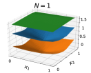
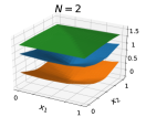
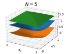
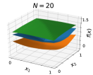
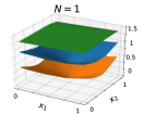
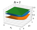
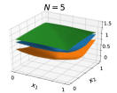
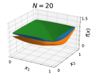
Figure 1: Hierarchical relaxations from $N=1$ (equiv. big-M) to $N=20$ (convex hull of each node over a box domain) for a two-input ($x_{1},x_{2}$) NN trained on scaled Ackley function, with output $f(\boldsymbol{x})$. Top row: $z_{n}^{b}$ bounds obtained using interval arithmetic; Bottom row: $z_{n}^{b}$ bounds obtained by optimization-based bound tightening. The partitions are formed using the equal size strategy.

Optimization-Based Bound Tightening (OBBT) or progressive bounds tightening [33], tightens variable bounds and constraints [15]. For example, solving the optimization problem with the objective set to minimize/maximize $(\boldsymbol{w}^{T}\boldsymbol{x}+b)$ gives bounds: $\mathrm{min}(\boldsymbol{w}^{T}\boldsymbol{x}+b)\leq\boldsymbol{w}^{T}\boldsymbol{x}+b\leq\mathrm{max}(\boldsymbol{w}^{T}\boldsymbol{x}+b)$. To simplify these problems, OBBT can be performed using the relaxed model (i.e., $\sigma\in[0,1]$ rather than $\sigma\in\{0,1\}$), resulting in a linear program (LP). In contrast to (26)–(27), bounds from OBBT incorporate variable dependencies. We apply OBBT by solving one LP per bound.

The partitioned formulation (21)–(25) requires bounds such that $z_{n}^{a}\in\sigma[\mathit{LB}_{n}^{a},\mathit{UB}_{n}^{a}]$, $z_{n}^{b}\in(1-\sigma)[\mathit{LB}_{n}^{b},\mathit{UB}_{n}^{b}]$. In other words, $[\mathit{LB}_{n}^{a},\mathit{UB}_{n}^{a}]$ is a valid domain for $z_{n}^{a}$ when the node is inactive ($\sigma=1$) and vice versa. These bounds can also be obtained via OBBT: $\mathrm{min}(\sum_{i\in\mathbb{S}_{n}}w_{i}x_{i})\leq z_{n}^{a}\leq\mathrm{max}(\sum_{i\in\mathbb{S}_{n}}w_{i}x_{i});\boldsymbol{w}^{T}\boldsymbol{x}+b\leq 0$. The constraint on the right-hand side of disjunction (20) can be similarly enforced in OBBT problems for $z_{n}^{b}$. In our framework, OBBT additionally captures dependencies within each partition $\mathbb{S}_{n}$. Specifically, we observe that the partitioned OBBT problems effectively form the convex hull over a given polyhedron of the input variables, in contrast to the convex hull formulation, which only considers the box domain defined by the min/max of each input node [3]. Since $\sum_{i\in\mathbb{S}_{n}}w_{i}x_{i}$ $=z_{n}^{a}+z_{n}^{b}$ and $z_{n}^{a}z_{n}^{b}=0$, the bounds $[\mathrm{min}(\sum_{i\in\mathbb{S}_{n}}w_{i}x_{i})$, $\mathrm{max}(\sum_{i\in\mathbb{S}_{n}}w_{i}x_{i})]$ are valid for both $z_{n}^{a}$ and $z_{n}^{b}$. These bounds can be from (26)–(27), or by solving two OBBT problems for each partition ($2N$ LPs total). This simplification uses equivalent bounds for $z_{n}^{a}$ and $z_{n}^{b}$, but tighter bounds can potentially be found by performing OBBT for $z_{n}^{a}$ and $z_{n}^{b}$ separately ($4N$ LPs total).

Figure 1 compares the proposed formulation with bounds from interval arithmetic (top row) vs OBBT (bottom row). The true model outputs (blue), and minimum (orange) and maximum (green) outputs of the relaxed model are shown over the input domain. The NNs comprise two inputs, three hidden layers with 20 nodes each, and one output. As expected, OBBT greatly improves relaxation tightness.

3.2 Tightness of the Proposed Formulation

Proposition 1.

(21)–(25) has the equivalent non-lifted (i.e., without auxiliary variables) formulation:

$$y\leq\sum_{i\in\mathcal{I}_{j}}w_{i}x_{i}+\sigma(b+\sum_{i\in\mathcal{I}\setminus\mathcal{I}_{j}}\mathit{UB}_{i})+(\sigma-1)(\sum_{i\in\mathcal{I}_{j}}\mathit{LB}_{i}), \forall j=1,...,2^{N}$$ (28)

$$y\geq\boldsymbol{w}^{T}\boldsymbol{x}+b$$ (29)

$$y\leq\sigma\mathit{UB}^{0}$$ (30)

where $\mathit{UB}_{i}$ and $\mathit{LB}_{i}$ denote the upper and lower bounds of $w_{i}x_{i}$. The set $\mathcal{I}$ denotes the input indices $\{1,...,\eta\}$, and the subset $\mathcal{I}_{j}$ denotes the indices contained by the union of the $j$-th combination of partitions in $\{\mathbb{S}_{1},...,\mathbb{S}_{N}\}$.

Proof.

Formulation (21)–(25) introduces $N$ auxiliary variables $z_{n}^{b}$, which can be projected out using Fourier-Motzkin elimination (appendix A.2), resulting in combinations $\mathcal{I}_{1},...,\mathcal{I}_{J},J=2^{N}$. ∎

Remark.

When $N<\eta$, the family of constraints in (28) represent a subset of the inequalities used to define the convex hull by Anderson et al. [3], where $\mathit{UB}_{i}$ and $\mathit{LB}_{i}$ would be obtained using interval arithmetic. Therefore, though a lifted formulation is proposed in this work, the proposed formulations have non-lifted relaxations equivalent to pre-selecting a subset of the convex hull inequalities.

Proposition 2.

Formulation (21)–(25) is equivalent to the big-M formulation (2)–(4) when $N=1$ .

Proof.

When $N=1$, it follows that $\mathbb{S}_{1}=\{1,..,\eta\}$. Therefore, $z_{1}=\sum_{i=1}^{\eta}w_{i}x_{i}=\boldsymbol{w}^{T}\boldsymbol{x}$, and $\sum_{n}z_{n}=z_{1}=z$. Conversely, big-M can be seen as the convex hull over a single aggregated “variable,” $z=\boldsymbol{w}^{T}\boldsymbol{x}$. ∎

Proposition 3.

Formulation (21)–(25) represents the convex hull of (1), given the inputs $\boldsymbol{x}$ are bounded, for the case of $N=\eta$.

Proof.

When $N=\eta$, it follows that $\mathbb{S}_{n}=\{n\},\forall n=1,..,\eta$, and, consequently, $z_{n}=w_{n}x_{n}$. Since $z_{n}$ are linear transformations of each $x_{n}$ (as are their respective bounds), forming the convex hull over $z_{n}$ recovers the convex hull over $\boldsymbol{x}$. An extended proof is provided in appendix A.3. ∎

Proposition 4.

A formulation with $N$ partitions is strictly tighter than any formulation with $(N-1)$ partitions that is derived by combining two partitions in the former.

Proof.

When combining two partitions, i.e., $\mathbb{S}^{\prime}_{N-1}:=\mathbb{S}_{N-1}\cup\mathbb{S}_{N}$, constraints in (28) where $\mathbb{S}^{\prime}_{N-1}\subseteq\mathcal{I}_{j}$ are also obtained by $\{\mathbb{S}_{N-1},\mathbb{S}_{N}\}\subseteq\mathcal{I}_{j}$. In contrast, those obtained by $\mathbb{S}_{N-1}\lor\mathbb{S}_{N}\subseteq\mathcal{I}_{j}$ cannot be modeled by $\mathbb{S}^{\prime}_{N-1}$. Since each constraint in (28) is facet-defining [3] and distinct from each other, omissions result in a less tight formulation. ∎

Remark.

The convex hull can be formulated with $\eta$ auxiliary variables (74)–(79), or $2^{\eta}$ constraints (28). While these formulations have tighter relaxations, they can perform worse than big-M due to having more difficult branch-and-bound subproblems. Our proposed formulation balances this tradeoff by introducing a hierarchy of relaxations with increasing tightness and size. The convex hull is created over partitions $z_{n},n=1,...,N$, rather than the input variables $x_{n},n=1,...,\eta$. Therefore, only $N$ auxiliary variables are introduced, with $N\leq\eta$. The results in this work are obtained using this lifted formulation (21)–(25); Appendix A.5 compares the computational performance of equivalent non-lifted formulations, i.e., involving $2^{N}$ constraints.

Figure 1 shows a hierarchy of increasingly tight formulations from $N=1$ (equiv. big-M ) to $N=20$ (convex hull of each node over a box input domain). The intermediate formulations approximate the convex-hull ($N=20$) formulation well, but need fewer auxiliary variables/constraints.

3.3 Effect of Input Partitioning Choice

Formulation (21)–(25) creates the convex hull over $z_{n}=\sum_{i\in\mathbb{S}_{n}}w_{i}x_{i},n=1,...,N$. The hyperparameter $N$ dictates model size, and the choice of subsets, $\mathbb{S}_{1},...,\mathbb{S}_{N}$, can strongly impact the strength of its relaxation. By Proposition 4, (21)–(25) can in fact give multiple hierarchies of formulations. While all hierarchies eventually converge to the convex hull, we are primarily interested in those with tight relaxations for small $N$.

Bounds and Bounds Tightening. Bounds on the partitions play a key role in the proposed formulation. For example, consider when a node is inactive: $\sigma=1$, $z_{n}^{b}=0$, and (24) gives the bounds $\sigma LB_{n}^{a}\leq\sum_{i\in\mathbb{S}_{n}}w_{i}x_{i}\leq\sigma UB_{n}^{a}$. Intuitively, the proposed formulation represents the convex hull over the auxiliary variables, $z_{n}=\sum_{i\in\mathbb{S}_{n}}w_{i}x_{i}$, and their bounds play a key role in model tightness. We hypothesize these bounds are most effective when partitions $\mathbb{S}_{n}$ are selected such that $w_{i}x_{i},\forall i\in\mathbb{S}_{n}$ are of similar orders of magnitude. Consider for instance the case of $\boldsymbol{w}=[1,1,100,100]$ and $x_{i}\in[0,1],i=1,...,4$. As all weights are positive, interval arithmetic gives $0\leq\sum x_{i}w_{i}\leq\sum\bar{x}_{i}w_{i}$. With two partitions, the choices of $\mathbb{S}_{1}=\{1,2\}$ vs $\mathbb{S}_{1}=\{1,3\}$ give:

$$\left[\begin{array}[]{c}x_{1}+x_{2}\leq\sigma 2\\ x_{3}+x_{4}\leq\sigma 2\end{array}\right]\mathrm{vs.}\left[\begin{array}[]{c}x_{1}+100x_{3}\leq\sigma 101\\ x_{2}+100x_{4}\leq\sigma 101\end{array}\right]$$ (31)

where $\sigma$ is a binary variable. The constraints on the right closely approximate the $\eta$-partition (i.e., convex hull) bounds: $x_{3}\leq\sigma$ and $x_{4}\leq\sigma$. But $x_{1}$ and $x_{2}$ are relatively unaffected by a perturbation $\sigma=1-\delta$ (when $\sigma$ is relaxed). Whereas the formulation on the left constrains the four variables equivalently. If the behavior of the node is dominated by a few inputs, the formulation on the right is strong, as it approximates the convex hull over those inputs ($z_{1}\approx x_{3}$ and $z_{2}\approx x_{4}$ in this case). For the practical case of $N<<\eta$, there are likely fewer partitions than dominating variables.

The size of the partitions can also be selected to be uneven:

$$\left[\begin{array}[]{c}x_{1}\leq\sigma 1\\ x_{2}+100x_{3}+100x_{4}\leq\sigma 201\end{array}\right]\mathrm{vs.}\left[\begin{array}[]{c}x_{3}\leq\sigma 1\\ x_{1}+x_{2}+100x_{4}\leq\sigma 102\end{array}\right]$$ (32)

Similar tradeoffs are seen here: the first formulation provides the tightest bound for $x_{1}$, but $x_{2}$ is effectively unconstrained and $x_{3},x_{4}$ approach “equal treatment.” The second formulation provides the tightest bound for $x_{3}$, and a tight bound for $x_{4}$, but $x_{1},x_{2}$ are effectively unbounded for fractional $\sigma$. The above analyses also apply to the case of OBBT. For the above example, solving a relaxed model for $\mathrm{max}(x_{1}+x_{2})$ obtains a bound that affects the two variables equivalently, while the same procedure for $\mathrm{max}(x_{1}+100x_{3})$ obtains a bound that is much stronger for $x_{3}$ than for $x_{1}$. Similarly, $\mathrm{max}(x_{1}+x_{2})$ captures dependency between the two variables, while $\mathrm{max}(x_{1}+100x_{3})\approx\mathrm{max}(100x_{3})$.

Relaxation Tightness. The partitions (and their bounds) also directly affect the tightness of the relaxation for the output variable $y$. The equivalent non-lifted realization (28) reveals the tightness of the above simple example. With two partitions, the choices of $\mathbb{S}_{1}=\{1,2\}$ vs $\mathbb{S}_{1}=\{1,3\}$ result in the equivalent non-lifted constraints:

$$\left[\begin{array}[]{c}y\leq x_{1}+100x_{3}+\sigma(b+101)\\ y\leq x_{2}+100x_{4}+\sigma(b+101)\end{array}\right]\mathrm{vs.}\left[\begin{array}[]{c}y\leq x_{1}+x_{2}+\sigma(b+200)\\ y\leq 100x_{3}+100x_{4}+\sigma(b+2)\end{array}\right]$$ (33)

Note that combinations $\mathcal{I}_{j}=\emptyset$ and $\mathcal{I}_{j}=\{1,2,3,4\}$ in (28) are not analyzed here, as they correspond to the big-M/1-partition model and are unaffected by choice of partitions. The 4-partition model is the tightest formulation and (in addition to all possible 2-partition constraints) includes:

$$y \leq x_{i}+\sigma(b+201),i=1,2$$ (34)

$$y \leq 100x_{i}+\sigma(b+102),i=3,4$$ (35)

The unbalanced 2-partition, i.e., the left of (33), closely approximates two of the $4$-partition (i.e., convex hull) constraints (35). Analogous to the tradeoffs in terms of bound tightness, we see that this formulation essentially neglects the dependence of $y$ on $x_{1},x_{2}$ and instead creates the convex hull over $z_{1}=x_{1}+100x_{3}\approx x_{3}$ and $z_{2}\approx x_{4}$. For this simple example, the behavior of $y$ is dominated by $x_{3}$ and $x_{4}$, and this turns out to be a relatively strong formulation. However, when $N<<\eta$, we expect neglecting the dependence of $y$ on some input variables to weaken the model.

The alternative formulation, i.e., the right of (33), handles the four variables similarly and creates the convex hull in two new directions: $z_{1}=x_{1}+x_{2}$ and $z_{2}=100(x_{3}+x_{4})$. While this does not model the individual effect of either $x_{3}$ or $x_{4}$ on $y$ as closely, it includes dependency between $x_{3}$ and $x_{4}$. Furthermore, $x_{1}$ and $x_{2}$ are modeled equivalently (i.e., less tightly than individual constraints). Analyzing partitions with unequal size reveals similar tradeoffs. This section shows that the proposed formulation has a relaxation equivalent to selecting a subset of constraints from (28), with a tradeoff between modeling the effect of individual variables well vs the effect of many variables weakly.

Deriving Cutting Planes from Convex Hull. The convex-hull constraints (28) not implicitly modeled by a partition-based formulation can be viewed as potential tightening constraints, or cuts. Anderson et al. [3] provide a linear-time method for selecting the most violated of the exponentially many constraints (28), which is naturally compatible with our proposed formulation (some constraints will be always satisfied). Note that the computational expense can still be significant for practical instances; Botoeva et al. [5] found adding cuts to $<$0.025% of branch-and-bound nodes to balance their expense and tightening, while De Palma et al. [13] proposed adding cuts at the root node only.

Remark.

While the above 4-D case may seem to favor “unbalanced” partitions, it is difficult to illustrate the case where $N<<\eta$. Our experiments confirm “balanced” partitions perform better.

3.4 Strategies for Selecting Partitions

The above rationale motivates selecting partitions that result in a model that treats input variables (approximately) equivalently for the practical case of $N<<\eta$. Specifically, we seek to evenly distribute tradeoffs in model tightness among inputs. Section 3.3 suggests a reasonable approach is to select partitions such that weights in each are approximately equal (weights are fixed during optimization). We propose two such strategies below, as well as two strategies in red for comparison.

Equal-Size Partitions. One strategy is to create partitions of equal size, i.e., $|\mathbb{S}_{1}|=|\mathbb{S}_{2}|=...=|\mathbb{S}_{N}|$ (note that they may differ by up to one if $\eta$ is not a multiple of $N$). Indices are then assigned to partitions to keep the weights in each as close as possible. This is accomplished by sorting the weights $\boldsymbol{w}$ and distributing them evenly among partitions (array_split(argsort($\boldsymbol{w}$), $N$) in Numpy).

Equal-Range Partitions. A second strategy is to partition with equal range, i.e., $\underset{i\in\mathbb{S}_{1}}{\mathrm{range}}(w_{i})=...=\underset{i\in\mathbb{S}_{N}}{\mathrm{range}}(w_{i})$. We define thresholds $\boldsymbol{v}\in\mathbb{R}^{N+1}$ such that $v_{1}$ and $v_{N+1}$ are $\mathrm{min}(\boldsymbol{w})$ and $\mathrm{max}(\boldsymbol{w})$. To reduce the effect of outliers, we define $v_{2}$ and $v_{N}$ as the 0.05 and 0.95 quantiles of $\boldsymbol{w}$, respectively. The remaining elements of $\boldsymbol{v}$ are distributed evenly in $(v_{2},v_{N})$. Indices $i\in\{1,...,\eta\}$ are then assigned to $\mathbb{S}_{n}:w_{i}\in[v_{n},v_{n+1})$. This strategy requires $N\geq 3$, but, for a symmetrically distributed weight vector, $\boldsymbol{w}$, two partitions of equal size are also of equal range.

We compare our proposed strategies against the following:

Random Partitions. Input indices $\{1,...,\eta\}$ are assigned randomly to partitions $\mathbb{S}_{1},...,\mathbb{S}_{N}$.

Uneven Magnitudes. Weights are sorted and “dealt” in reverse to partitions in snake-draft order.

4 Experiments

Computational experiments were performed using Gurobi v 9.1 [19]. The computational set-up, solver settings, and models for MNIST [22] and CIFAR-10 [20] are described in appendix A.4.

4.1 Optimal Adversary Results

The optimal adversary problem takes a target image $\bar{\boldsymbol{x}}$, its correct label $j$, and an adversarial label $k$, and finds the image within a range of perturbations maximizing the difference in predictions. Mathematically, this is formulated as $\underset{\boldsymbol{x}}{\mathrm{max}}(f_{k}(\boldsymbol{x})-f_{j}(\boldsymbol{x}));x\in\mathcal{X}$, where $f_{k}$ and $f_{j}$ correspond to the $k$- and $j$-th elements of the NN output layer, respectively, and $\mathcal{X}$ defines the domain of perturbations. We consider perturbations defined by the $\ell_{1}$-norm ($||\boldsymbol{x}-\bar{\boldsymbol{x}}||_{1}\leq\epsilon_{1}\in\mathbb{R}$), which promotes sparse perturbations [8]. For each dataset, we use the first 100 test-dataset images and randomly selected adversarial labels (the same 100 instances are used for models trained on the same dataset).

Table 1: Number of solved (in 3600s) optimal adversary problems and average solve times for big-M vs $N=\{2,4\}$ equal-size partitions. Average times computed for problems solved by all 3 formulations. Grey indicates partition formulations strictly outperforming big-M.

Dataset	Model	$\epsilon_{1}$	Big-M		2 Partitions		4 Partitions
			solved	avg.time(s)	solved	avg.time(s)	solved	avg.time(s)
MNIST	$2\times 50$	5	100	57.6	100	42.7	100	83.9
	$2\times 50$	10	97	431.8	98	270.4	98	398.4
	$2\times 100$	2.5	92	525.2	100	285.1	94	553.9
	$2\times 100$	5	38	1587.4	59	587.8	48	1084.7
	CNN1*	0.25	68	1099.7	86	618.8	87	840.0
	CNN1*	0.5	2	2293.2	16	1076.0	11	2161.2
CIFAR-10	$2\times 100$	5	62	1982.3	69	1083.4	85	752.8
	$2\times 100$	10	23	2319.0	28	1320.2	34	1318.1

*OBBT performed on all NN nodes

Table 1 gives the optimal adversary results. Perturbations $\epsilon_{1}$ were selected such that some big-M problems were solvable within 3600s (problems become more difficult as $\epsilon_{1}$ increases). While our formulations consistently outperform big-M in terms of problems solved and solution times, the best choice of $N$ is problem-dependent. For instance, the 4-partition formulation performs best for the $2\times 100$ network trained on CIFAR-10; Figure 2 (right) shows the number of problems solved for this case. The 2-partition formulation is best for easy problems, but is soon overtaken by larger values of $N$. Intuitively, simpler problems are solved with fewer branch-and-bound nodes and benefit more from smaller subproblems. Performance declines again near $N\geq 7$, supporting observations that the convex-hull formulation ($N=\eta$) is not always best [3].

Convex-Hull-Based Cuts. The cut-generation strategy for big-M by Anderson et al. [3] is compatible with our formulations (Section 3.3), i.e., we begin with a partition-based formulation and apply cuts during optimization. Figure 2 (left) gives results with these cuts added (via Gurobi callbacks) at various cut frequencies. Specifically, a cut frequency of $1/k$ corresponds to adding the most violated cut (if any) to each NN node at every $k$ branch-and-bound nodes. Performance is improved at certain frequencies; however, our formulations consistently outperform even the best cases using big-M with cuts. Moreover, cut generation is not always straightforward to integrate with off-the-shelf MILP solvers, and our formulations often perform just as well (if not better) without added cuts. Appendix A.5 gives results with most-violated cuts directly added to the model, as in De Palma et al. [13].

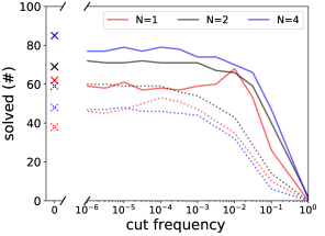
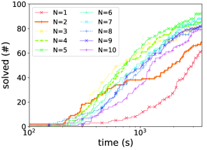
Figure 2: Number solved vs convex-hull-cut frequency/run time for optimal adversary problems ($\epsilon=5$) for $2\times 100$ models, without OBBT. Left: $N=1$ (equivalent to big-M) performs worst on MNIST (dotted) and CIFAR-10 (solid) models for most cut frequencies. Right: each line shows 100 runs of CIFAR-10 model (no convex-hull cuts). $N=1$ performs the worst; $N=2$ performs well for easier problems; and intermediate values of $N$ balance model size and tightness well.

Partitioning Strategies. Figure 3 shows the result of the input partitioning strategies from Section 3.4 on the MNIST $2\times 100$ model for varying $N$. Both proposed strategies ( blue) outperform formulations with random and uneven partitions ( red). With OBBT, big-M ($N=1$) outperforms partition-based formulations when partitions are selected poorly. Figure 3 again shows that our formulations perform best for some intermediate $N$; random/uneven partitions worsen with increasing $N$.

   

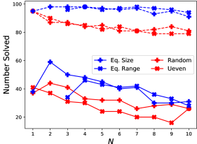
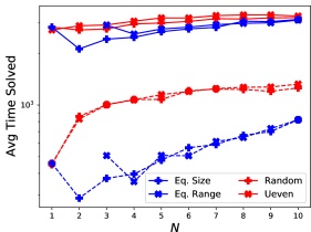
Figure 3: Number solved (left) and solution times (right) for optimal adversary problems for MNIST $2\times 100$ ($\epsilon=5$). Each point shows 100 runs, max time of 3600s. Dashed lines show runs with OBBT. The equal range strategy requires $N\geq 3$. Our proposed ( blue) partitioning strategies solve more problems (top) faster (bottom) than random and uneven partitions ( red)

Optimization-Based Bounds Tightening. OBBT was implemented by tightening bounds for all $z_{n}^{b}$. We found that adding the bounds from the 1-partition model (i.e., bounds on $\sum z_{n}^{b}$) improved all models, as they account for dependencies among all inputs. Therefore these bounds were used in all models, resulting in $2N+2$ LPs per node ($N\geq 2$). We limited the OBBT LPs to 5s; interval bounds were used if an LP was not solved. Figure 3 shows that OBBT greatly improves the optimization performance of all formulations. OBBT problems for each layer are independent and could, in practice, be solved in parallel. Therefore, at a minimum, OBBT requires the sum of max solution times found in each layer (5s $\times$ # layers in this case). This represents an avenue to significantly improve MILP optimization of NNs via parallelization. In contrast, parallelizing branch-and-bound is known to be challenging and may have limited benefits [1, 26].

Table 2: Number of verification problems solved in 3600s and average solve times for big-M vs $N=\{2,\,4\}$ equal-size partitions. Average times computed for problems solved by all 3 formulations. OBBT was performed for all problems. Grey indicates formulations strictly outperforming big-M.

Dataset	Model	$\epsilon_{\infty}$	Big-M		2 Partitions		4 Partitions
			sol.(#)	avg.time(s)	sol.(#)	avg.time(s)	sol.(#)	avg.time(s)
MNIST	CNN1	0.050	82	198.5	92	27.3	90	52.4
	CNN1	0.075	30	632.5	52	139.6	42	281.6
	CNN2	0.075	21	667.1	36	160.7	31	306.0
	CNN2	0.100	1	505.3	5	134.7	5	246.3
CIFAR-10	CNN1	0.007	99	100.6	100	25.9	99	45.4
	CNN1	0.010	98	119.1	100	25.7	100	45.0
	CNN2	0.007	80	300.5	95	85.1	68	928.6
	CNN2	0.010	40	743.6	72	176.4	35	1041.3

4.2 Verification Results

The verification problem is similar to the optimal adversary problem, but terminates when the sign of the objective function is known (i.e., the lower/upper bounds of the MILP have the same sign). This problem is typically solved for perturbations defined by the $\ell_{\infty}$-norm ($||\boldsymbol{x}-\bar{\boldsymbol{x}}||_{\infty}\leq\epsilon_{\infty}\in\mathbb{R}$). Here, problems are difficult for moderate $\epsilon_{\infty}$: at large $\epsilon_{\infty}$ a mis-classified example (positive objective) is easily found. Several verification tools rely on an underlying big-M formulation, e.g., MIPVerify [33], NSVerify [2], making big-M an especially relevant point of comparison. Owing to the early termination, larger NNs can be tested compared to the optimal adversary problems. We turned off cuts (cuts$=0$) for the partition-based formulations, as the models are relatively tight over the box-domain perturbations and do not seem to benefit from additional cuts. On the other hand, removing cuts improved some problems using big-M and worsened others. Results are presented in Table 2. Our formulations again generally outperform big-M ($N$=1), except for a few of the 4-partition problems.

Table 3: Number of $\ell_{1}$-minimally distorted adversary problems solved in 3600s and average solve times for big-M vs $N=\{2,\,4\}$ equal-size partitions. Average times and $\epsilon_{1}$ are computed for problems solved by all 3 formulations. OBBT was performed for all problems. Grey indicates partition formulations strictly outperforming big-M.

Dataset	Model	$\mathrm{avg}(\epsilon_{1})$	Big-M		2 Partitions		4 Partitions
			solved	avg.time(s)	solved	avg.time(s)	solved	avg.time(s)
MNIST	$2\times 50$	6.51	52	675.0	93	150.9	89	166.6
	$2\times 75$	4.41	16	547.3	37	310.5	31	424.0
	$2\times 100$	2.73	7	710.8	13	572.9	10	777.9

4.3 Minimally Distorted Adversary Results

In a similar vein as Croce and Hein [11], we define the $\ell_{1}$-minimally distorted adversary problem: given a target image $\bar{\boldsymbol{x}}$ and its correct label $j$, find the smallest perturbation over which the NN predicts an adversarial label $k$. We formulate this as $\underset{\epsilon_{1},\boldsymbol{x}}{\mathrm{min}}\ \epsilon_{1};||\boldsymbol{x}-\bar{\boldsymbol{x}}||_{1}\leq\epsilon_{1};f_{k}(\boldsymbol{x})\geq f_{j}(\boldsymbol{x})$. The adversarial label $k$ is selected as the second-likeliest class of the target image. Figure 4 provides examples illustrating that the $\ell_{1}$-norm promotes sparse perturbations, unlike the $\ell_{\infty}$-norm. Note that the sizes of perturbations $\epsilon_{1}$ are dependent on input dimensionality; if it were distributed evenly, $\epsilon_{1}=5$ would correspond to an $\ell_{\infty}$-norm perturbation $\epsilon_{\infty}\approx 0.006$ for MNIST models.

Figure 4: Sample $\ell_{1}$- vs $\ell_{\infty}$-based minimally distorted adversaries for the MNIST $2\times 50$ model. The true label ($j$) is ‘9,’ and the adversarial label ($k$) is ‘4.’

Table 3 presents results for the minimally distorted adversary problems. As input domains are unbounded, these problems are considerably more difficult than the above optimal adversary problems. Therefore, only smaller MNIST networks were manageable (with OBBT) for all formulations. Again, partition-based formulations consistently outperform big-M, solving more problems and in less time.

5 Conclusions

This work presented MILP formulations for ReLU NNs that balance having a tight relaxation and manageable size. The approach forms the convex hull over partitions of node inputs; we presented theoretical and computational motivations for obtaining good partitions for ReLU nodes. Furthermore, our approach expands the benefits of OBBT, which, unlike conventional MILP tools, can easily be parallelized. Results on three classes of optimization tasks show that the proposed formulations consistently outperform standard MILP encodings, allowing us to solve 25% more of the problems (average $>$2X speedup for solved problems). Implementations of the proposed formulations and partitioning strategies are available at https://github.com/cog-imperial/PartitionedFormulations_NN.

Appendix A Appendix

A.1 Derivation of Proposed Formulation

Given the disjunction:

$$\left[\begin{array}[]{c}y=0\\ \sum_{n=1}^{N}z_{n}+b\leq 0\end{array}\right]\lor\left[\begin{array}[]{c}y=\sum_{n=1}^{N}z_{n}+b\\ y\leq 0\end{array}\right]$$ (40)

The extended, or “multiple choice,” formulation for disjunctions [4] introduces auxiliary variables $z_{n}^{a}$ and $z_{n}^{b}$ for each $z_{n}$:

$$\sum_{i\in\mathbb{S}_{n}}w_{i}x_{i}=z_{n}^{a}+z_{n}^{b}$$ (41)

$$\sum_{n}z_{n}^{a}+\sigma b\leq 0$$ (42)

$$\sum_{n}z_{n}^{b}+(1-\sigma)b\geq 0$$ (43)

$$y=\sum_{n}z_{n}^{b}+(1-\sigma)b$$ (44)

$$\sigma\mathit{LB}_{n}^{a}\leq z_{n}^{a}\leq\sigma\mathit{UB}_{n}^{a}, \forall n=1,...,N$$ (45)

$$(1-\sigma)\mathit{LB}_{n}^{b}\leq z_{n}^{b}\leq(1-\sigma)\mathit{UB}_{n}^{b}, \forall n=1,...,N$$ (46)

where again $\sigma\in\{0,1\}$. We observe that (41)–(46) exactly represents the ReLU node described by (20): substituting $z_{n}=\sum_{i\in\mathbb{S}_{n}}w_{i}x_{i}$ in the extended convex hull formulation [4] of the original disjunction (9), directly gives (41)–(46). Eliminating $z_{n}^{a}$ via (41) results in our proposed formulation:

$$\sum_{n}\left(\sum_{i\in\mathbb{S}_{n}}w_{i}x_{i}-z_{n}^{b}\right)+\sigma b\leq 0$$ (47)

$$\sum_{n}z_{n}^{b}+(1-\sigma)b\geq 0$$ (48)

$$y=\sum_{n}z_{n}^{b}+(1-\sigma)b$$ (49)

$$\sigma\mathit{LB}_{n}^{a}\leq\sum_{i\in\mathbb{S}_{n}}w_{i}x_{i}-z_{n}^{b}\leq\sigma\mathit{UB}_{n}^{a}, \forall n=1,...,N$$ (50)

$$(1-\sigma)\mathit{LB}_{n}^{b}\leq z_{n}^{b}\leq(1-\sigma)\mathit{UB}_{n}^{b}, \forall n=1,...,N$$ (51)

A.2 Derivation of Equivalent Non-Extended Formulation

We seek an equivalent (non-lifted) formulation to (47)–(51) without $z_{n}^{b}$. The term $\sum_{n}z_{n}^{b}$ can be isolated in (47)–(49), giving:

$$\sum_{n}z_{n}^{b} \geq\boldsymbol{w}^{T}\boldsymbol{x}+\sigma b$$ (52)

$$\sum_{n}z_{n}^{b} \geq-(1-\sigma)b$$ (53)

$$\sum_{n}z_{n}^{b} =y-(1-\sigma)b$$ (54)

We observed in Section 3.1 that $[\mathrm{min}(\sum_{i\in\mathbb{S}_{n}}w_{i}x_{i})$, $\mathrm{max}(\sum_{i\in\mathbb{S}_{n}}w_{i}x_{i})]$ are valid for both $z_{n}^{a}$ and $z_{n}^{b}$. Let $\mathit{UB}_{i}$ and $\mathit{LB}_{i}$ denote, respectively, valid upper and lower bounds of weighted input $w_{i}x_{i}$. Isolating $z_{n}^{b}$ in the bounds (50)–(51) gives:

$$z_{n}^{b} \leq\sum_{i\in\mathbb{S}_{n}}w_{i}x_{i}-\sigma\sum_{i\in\mathbb{S}_{n}}\mathit{LB}_{i}$$ (55)

$$z_{n}^{b} \geq\sum_{i\in\mathbb{S}_{n}}w_{i}x_{i}-\sigma\sum_{i\in\mathbb{S}_{n}}\mathit{UB}_{i}$$ (56)

$$z_{n}^{b} \leq(1-\sigma)\sum_{i\in\mathbb{S}_{n}}\mathit{UB}_{i}$$ (57)

$$z_{n}^{b} \geq(1-\sigma)\sum_{i\in\mathbb{S}_{n}}\mathit{LB}_{i}$$ (58)

Fourier-Motzkin Elimination. We will now eliminate the auxiliary variables using the above inequalities. Equations that appear in the non-extended formulation are marked in green. First, we examine the equations containing $\sum_{n}z_{n}^{b}$. Combining (52)+(54) and (53)+(54) gives, respectively:

$$\color[rgb]{0.1953125,0.51171875,0.1953125}y \color[rgb]{0.1953125,0.51171875,0.1953125}\geq\boldsymbol{w}^{T}\boldsymbol{x}+b$$ (59)

$$\color[rgb]{0.1953125,0.51171875,0.1953125}y \color[rgb]{0.1953125,0.51171875,0.1953125}\geq 0$$ (60)

Secondly, we examine equations containing only $z_{n}^{b}$. Combining (55)+(56) gives the trivial constraint $\sum_{i\in\mathbb{S}_{n}}UB_{i}\geq\sum_{i\in\mathbb{S}_{n}}LB_{i}$. Combining (57)+(58) gives the same constraint. The other combinations (55)+(58) and (56)+(57) recover the definition of lower and upper bounds on the partitions:

$$\sum_{i\in\mathbb{S}_{n}}\mathit{LB}_{i} \leq\sum_{i\in\mathbb{S}_{n}}w_{i}x_{i}\leq\sum_{i\in\mathbb{S}_{n}}\mathit{UB}_{i}$$ (61)

Now examining both equations containing $z_{n}^{b}$ and those containing $\sum_{n}z_{n}^{b}$, the combinations between (54) and (55)–(58) are most interesting. Here, each $z_{n}^{b}$ can be eliminated using either inequality (55) or (57). Note that combining these with (52) or (53) results in trivially redundant constraints. Defining $\mathcal{A}$ as the indices of partitions for which (55) is used, and $\mathcal{B}$ as the remaining indices:

$$y-(1-\sigma)b\leq\sum_{n\in\mathcal{A}}\sum_{i\in\mathcal{S}_{n}}w_{i}x_{i}-\sigma\sum_{n\in\mathcal{A}}\sum_{i\in\mathcal{S}_{n}}\mathit{LB}_{i}+(1-\sigma)\sum_{n\in\mathcal{B}}\sum_{i\in\mathcal{S}_{n}}UB_{i}$$ (62)

Similarly, the inequalities of opposite sign can be chosen from either (56) or (58). Defining now $\mathcal{A}^{\prime}$ as the indices of partitions for which (56) is used, and $\mathcal{B}^{\prime}$ as the remaining indices:

$$y-(1-\sigma)b\geq\sum_{n\in\mathcal{A}^{\prime}}\sum_{i\in\mathcal{S}_{n}}w_{i}x_{i}-\sigma\sum_{n\in\mathcal{A}^{\prime}}\sum_{i\in\mathcal{S}_{n}}\mathit{UB}_{i}+(1-\sigma)\sum_{n\in\mathcal{B}}\sum_{i\in\mathcal{S}_{n}}LB_{i}$$ (63)

Defining $\mathcal{I}_{j}$ as the union of $\mathbb{S}_{n}\forall n\in\mathcal{A}$ and $\mathcal{I}_{j}^{\prime}$ as the union of $\mathbb{S}_{n}\forall n\in\mathcal{A}^{\prime}$, (62)–(63) become:

$$y \leq\sum_{i\in\mathcal{I}_{j}}w_{i}x_{i}-\sigma\sum_{i\in\mathcal{I}_{j}}\mathit{LB}_{i}+(1-\sigma)(b+\sum_{i\in\mathcal{I}\setminus\mathcal{I}_{j}}\mathit{UB}_{i})$$ (64)

$$y \geq\sum_{i\in\mathcal{I}_{j}^{\prime}}w_{i}x_{i}-\sigma\sum_{i\in\mathcal{I}_{j}^{\prime}}\mathit{UB}_{i}+(1-\sigma)(b+\sum_{i\in\mathcal{I}\setminus\mathcal{I}_{j}^{\prime}}\mathit{LB}_{i})$$ (65)

The lower inequality (65) is redundant. Consider that $\sigma\in\{0,1\}$. For $\sigma=0$ and $\sigma=1$, we recover:

$$y \geq\sum_{i\in\mathcal{I}_{j}^{\prime}}w_{i}x_{i}+(b+\sum_{i\in\mathcal{I}\setminus\mathcal{I}_{j}^{\prime}}\mathit{LB}_{i})$$ (66)

$$y \geq\sum_{i\in\mathcal{I}_{j}^{\prime}}(w_{i}x_{i}-\mathit{UB}_{i})$$ (67)

The former is less tight than $y\geq\boldsymbol{w}^{T}\boldsymbol{x}+b$, while the latter is less tight than $y\geq 0$. Finally, setting $\sigma^{\prime}=1-\sigma$ in (64) gives:

$$\color[rgb]{0.1953125,0.51171875,0.1953125}y \color[rgb]{0.1953125,0.51171875,0.1953125}\leq\sum_{i\in\mathcal{I}_{j}}w_{i}x_{i}+(\sigma^{\prime}-1)\sum_{i\in\mathcal{I}_{j}}\mathit{LB}_{i}+\sigma^{\prime}(b+\sum_{i\in\mathcal{I}\setminus\mathcal{I}_{j}}\mathit{UB}_{i})$$ (68)

The combination $\mathcal{I}_{j}=\emptyset$ removes all $x_{i}$, giving an upper bound for $y$:

$$\color[rgb]{0.1953125,0.51171875,0.1953125}y\leq\sigma^{\prime}(b+\sum_{i\in\mathcal{I}}\mathit{UB}_{i})$$ (69)

Combining all remaining equations gives a nonextended formulation:

$$y \leq\sum_{i\in\mathcal{I}_{j}}w_{i}x_{i}+\sigma^{\prime}(b+\sum_{i\in\mathcal{I}\setminus\mathcal{I}_{j}}\mathit{UB}_{i})+(\sigma^{\prime}-1)(\sum_{i\in\mathcal{I}_{j}}\mathit{LB}_{i})$$ (70)

$$y \geq\boldsymbol{w}^{T}\boldsymbol{x}+b$$ (71)

$$y \leq\sigma^{\prime}\mathit{UB}^{0}$$ (72)

$$y \in[0,\infty)$$ (73)

A.3 Equivalence of $\eta$-Partition Formulation to Convex Hull

When $N=\eta$, it follows that $\mathbb{S}_{n}=\{n\},\forall n=1,..,\eta$, and, consequently, $z_{n}=w_{n}x_{n}$. The auxiliary variables can be expressed in terms of $x_{n}$, rather of $z_{n}$ (i.e., $z_{n}^{a}=w_{n}x_{n}^{a}$ and $z_{n}^{b}=w_{n}x_{n}^{b}$). Rewriting (41)–(46) in this way gives:

$$x_{n}=x_{n}^{a}+x_{n}^{b}$$ (74)

$$\boldsymbol{w}^{T}\boldsymbol{x}^{a}+\sigma b\leq 0$$ (75)

$$\boldsymbol{w}^{T}\boldsymbol{x}^{b}+(1-\sigma)b\geq 0$$ (76)

$$y=\boldsymbol{w}^{T}\boldsymbol{x}^{b}+(1-\sigma)b$$ (77)

$$\sigma\frac{\mathit{LB}_{n}^{a}}{w_{n}}\leq x_{n}^{a}\leq\sigma\frac{\mathit{UB}_{n}^{a}}{w_{n}}, \forall n=1,...,\eta$$ (78)

$$(1-\sigma)\frac{\mathit{LB}_{n}^{b}}{w_{n}}\leq x_{n}^{b}\leq(1-\sigma)\frac{\mathit{UB}_{n}^{b}}{w_{n}}, \forall n=1,...,\eta$$ (79)

This formulation with a copy of each input—sometimes referred to as a “multiple choice” formulation—represents the convex hull of the node, e.g., see [3]; however, the overall model tightness still hinges on the bounds used for $x_{n},n=1,...,\eta$. We note that (78)–(79) are presented here with $x_{n}^{a}$ and $x_{n}^{b}$ isolated for clarity. In practice, the bounds can be written without $w_{n}$ in their denominators, as in (21)–(25).

A.4 Experiment Details

Computational Set-Up. All computational experiments were performed on a 3.2 GHz Intel Core i7-8700 CPU (12 threads) with 16 GB memory. Models were implemented and solved using Gurobi v 9.1 [19] (academic license). The LP algorithm was set to dual simplex, cuts $=1$ (moderate cut generation), TimeLimit $=3600s$, and default termination criteria were used. We set parameter MIPFocus $=3$ to ensure consistent solution approaches across formulations. Average times were computed as the arithmetic mean of solve times for instances solved by all formulations for a particular problem class. Thus, no time outs are included in the calculation of average solve times.

Neural Networks. We trained several NNs on MNIST [22] and CIFAR-10 [20], including both fully connected NNs and convolutional NNs (CNNs). MNIST (CC BY-SA 3.0) comprises a training set of 60,000 images and a test set of 10,000 images. CIFAR-10 (MIT License) comprises a training set of 50,000 images and a test set of 10,000 images. Dense models are denoted by $n_{\mathrm{Layers}}\times n_{\mathrm{Hidden}}$ and comprise $n_{\mathrm{Layers}}\times n_{\mathrm{Hidden}}$ hidden plus $10$ output nodes. CNN2 is based on ‘ConvSmall’ of the ERAN dataset [29]: {Conv2D(16, (4,4), (2,2)), Conv2D(32, (4,4), (2,2)), Dense(100), Dense(10)}. CNN1 halves the channels in each convolutional layer: {Conv2D(8, (4,4), (2,2)), Conv2D(16, (4,4), (2,2)), Dense(100), Dense(10)}. The implementations of CNN1/CNN2 have 1,852/3,604 and 2,476/4,852 nodes for MNIST and CIFAR-10, respectively. NNs are implemented in PyTorch [24] and obtained using standard training (i.e., without regularization or methods to improve robustness). MNIST models were trained for ten epochs, and CIFAR-10 models were trained for 20 epochs, all using the Adadelta optimizer with default parameters.

A.5 Additional Computational Results

Comparing formulations. Proposition 1 suggests an equivalent, non-lifted formulation for each partition-based formulation. In contrast to our proposed formulation (21)–(25), which adds a linear (w.r.t. number of partitions $N$) number of variables, this non-lifted formulation involves adding an exponential (w.r.t. $N$) number of constraints. Table 4 computationally compares our proposed formulations against non-lifted formulations with equivalent relaxations on 100 optimal adversary instances of medium difficulty. These results clearly show the advantages of the proposed formulations; a non-lifted formulation equivalent to 20-partitions (2²⁰ constraints per node) cannot even be fully generated on our test machines due to its computational burden. Additionally, our formulations naturally enable OBBT on partitions. As described in Section 3.1, this captures dependencies among each partition without additional constraints.

Table 4: Number of solved (in 3600s) optimal adversary problems for $N=\{2,5,10,20\}$ equal-size partitions for MNIST 2$\times$100 model, $\epsilon_{1}$=5. Performance is compared between proposed formulations and non-lifted formulations with equivalent relaxations.

Partitions	Proposed Formulation		Non-Lifted Formulation
$N$	solved	avg.time(s)	solved	avg.time(s)
2	59	530.1	41	1111.4
5	45	792.5	7	2329.8
10	31	-	0	-
20	22	-	0*	-

*The non-lifted formulation cannot be generated on our test machines.

As suggested in Proposition 1, the convex hull for a ReLU node involves an exponential (in terms of number of inputs) number of non-lifted constraints:

$$y \leq\sum_{i\in\mathcal{I}_{j}}w_{i}x_{i}+\sigma(b+\sum_{i\in\mathcal{I}\setminus\mathcal{I}_{j}}\mathit{UB}_{i})+(\sigma-1)(\sum_{i\in\mathcal{I}_{j}}\mathit{LB}_{i}), \forall j=1,...,2^{\eta}$$ (80)

where $\mathit{UB}_{i}$ and $\mathit{LB}_{i}$ denote the upper and lower bounds of $w_{i}x_{i}$. The set $\mathcal{I}$ denotes the input indices $\{1,...,\eta\}$, and the subset $\mathcal{I}_{j}$ contains the union of the $j$-th combination of partitions $\{\mathbb{S}_{1},...,\mathbb{S}_{\eta}\}$.

Anderson et al. [3] provide a linear-time method for identifying the most-violated constraint in (80). First, the subset $\hat{\mathcal{I}}$ is defined:

$$\hat{\mathcal{I}}=\Big{\{}i\in\mathcal{I}\ |\ w_{i}x_{i}<w_{i}\big{(}\mathit{LB}_{x_{i}}(1-\sigma)+\mathit{UB}_{x_{i}}\sigma\big{)}\Big{\}}$$ (81)

where $\mathit{LB}_{x_{i}}$ and $\mathit{UB}_{x_{i}}$ are, respectively, the lower and upper bounds of input $x_{i}$. Then, the constraint in (80) corresponding to the subset $\hat{\mathcal{I}}$ is checked:

$$y \leq\sum_{i\in\hat{\mathcal{I}}}w_{i}x_{i}+\sigma(b+\sum_{i\in\mathcal{I}\setminus\hat{\mathcal{I}}}\mathit{UB}_{i})+(\sigma-1)(\sum_{i\in\hat{\mathcal{I}}}\mathit{LB}_{i})$$ (82)

If this constraint (82) is violated, then it is the most violated in the family (80). If it is not, then no constraints in (80) are violated. This method can be used to solve the separation problem and generate cutting planes during optimization.

Figure 2 (left) shows that dynamically generated, convex-hull-based cuts only improve optimization performance when added at relatively low frequencies, if at all. Alternatively, De Palma et al. [13] only add the most violated cut (if one exists) at the initial LP solution to each node in the NN. Adding the cut before solving the MILP may produce different performance than dynamic cut generation: the De Palma et al. [13] approach to adding cuts includes the cut in the solver (Gurobi) pre-processing. Tables 5–8 give the results of the optimal adversary problem (cf. Table 1) with these single “most-violated” cuts added to each node. These cuts sometimes improve the big-M performance, but partition-based formulations still consistently perform best.

Table 5: Number of solved (in 3600s) optimal adversary problems for big-M vs $N=\{2,4\}$ equal-size partitions. Columns marked “w/cuts” denote most violated convex-hull cut at root MILP node added to each NN node. Most solved for each set of problems is in bold. Green text indicates more solved compared to no convex-hull cuts.

Dataset	Model	$\epsilon_{1}$	Big-M		2 Partitions		4 Partitions
			w/ cuts	w/o cuts	w/ cuts	w/o cuts	w/ cuts	w/o cuts
MNIST	$2\times 50$	5	100	100	100	100	100	100
	$2\times 50$	10	98	97	98	98	98	98
	$2\times 100$	2.5	95	92	100	100	97	94
	$2\times 100$	5	51	38	55	59	45	48
	CNN1*	0.25	91	68	85	86	83	87
	CNN1*	0.5	7	2	18	16	9	11
CIFAR-10	$2\times 100$	5	45	62	65	69	61	85
	$2\times 100$	10	11	23	30	28	26	34

*OBBT performed on all NN nodes

Table 6: Average solve times of optimal adversary problems for big-M vs $N=\{2,4\}$ equal-size partitions. Columns marked “w/cuts” denote most violated convex-hull cut at root MILP node added to each NN node. Average times computed for problems solved by all 6 formulations. Lowest average time for each set of problems is in bold. Green text indicates lower time compared to no convex-hull cuts.

Dataset	Model	$\epsilon_{\infty}$	Big-M		2 Partitions		4 Partitions
			w/ cuts	w/o cuts	w/ cuts	w/o cuts	w/ cuts	w/o cuts
MNIST	$2\times 50$	5	45.3	57.6	60.3	42.7	86.0	83.9
	$2\times 50$	10	285.2	431.8	305.0	270.4	404.5	398.4
	$2\times 100$	2.5	505.2	525.2	309.3	285.1	597.4	553.9
	$2\times 100$	5	930.5	1586.0	691.7	536.9	1131.4	1040.3
	CNN1*	0.25	420.7	1067.9	567.2	609.4	784.6	817.1
	CNN1*	0.5	1318.2	2293.2	1586.7	1076.0	1100.9	2161.2
CIFAR-10	$2\times 100$	5	1739.2	1914.6	595.1	1192.4	834.8	538.4
	$2\times 100$	10	1883.3	1908.9	1573.4	1621.4	1767.44	2094.5

*OBBT performed on all NN nodes

Table 7: Number of solved (in 3600s) verification problems for big-M vs $N=\{2,4\}$ equal-size partitions. OBBT was performed for all partitions, and columns marked “w/cuts” denote most violated convex-hull cut at root MILP node added to each NN node.. Most solved for each set of problems is in bold. Green text indicates more solved compared to no convex-hull cuts.

Dataset	Model	$\epsilon_{\infty}$	Big-M		2 Partitions		4 Partitions
			w/ cuts	w/o cuts	w/ cuts	w/o cuts	w/ cuts	w/o cuts
MNIST	CNN1	0.050	78	82	91	92	89	90
	CNN1	0.075	25	30	53	52	45	42
	CNN2	0.075	16	21	34	36	11	31
	CNN2	0.100	1	1	5	5	0	5
CIFAR-10	CNN1	0.007	98	99	100	100	99	99
	CNN1	0.010	80	98	94	100	89	100
	CNN2	0.007	78	80	94	95	73	68
	CNN2	0.010	29	40	74	72	34	35

Table 8: Average solve times of verification problems for big-M vs $N=\{2,4\}$ equal-size partitions. OBBT was performed for all partitions, and columns marked “w/cuts” denote most violated convex-hull cut at root MILP node added to each NN node. Average times computed for problems solved by all 6 formulations. Lowest average time for each set of problems is in bold. Green text indicates lower time compared to no convex-hull cuts.

Dataset	Model	$\epsilon_{1}$	Big-M		2 Partitions		4 Partitions
			w/ cuts	w/o cuts	w/ cuts	w/o cuts	w/ cuts	w/o cuts
MNIST	CNN1	0.050	133.7	92.2	20.4	19.3	37.2	33.3
	CNN1	0.075	504.7	239.0	155.8	84.4	178.2	161.2
	CNN2	0.075	637.8	414.8	101.9	95.4	901.3	175.1
	CNN2	0.100	-	-	-	-	-	-
CIFAR-10	CNN1	0.007	102.5	74.7	18.7	21.4	30.6	38.1
	CNN1	0.010	599.4	66.5	68.5	19.1	137.1	33.9
	CNN2	0.007	308.3	262.7	69.5	74.5	380.9	812.2
	CNN2	0.010	525.9	394.2	100.6	147.4	657.0	828.2

*OBBT performed on all NN nodes

References

- Achterberg and Wunderling [2013] Tobias Achterberg and Roland Wunderling. Mixed integer programming: Analyzing 12 years of progress. In Facets of Combinatorial Optimization, pages 449–481. Springer, 2013.
- Akintunde et al. [2018] Michael Akintunde, Alessio Lomuscio, Lalit Maganti, and Edoardo Pirovano. Reachability analysis for neural agent-environment systems. In International Conference on Principles of Knowledge Representation and Reasoning., pages 184–193, 2018.
- Anderson et al. [2020] Ross Anderson, Joey Huchette, Will Ma, Christian Tjandraatmadja, and Juan Pablo Vielma. Strong mixed-integer programming formulations for trained neural networks. Mathematical Programming, pages 1–37, 2020.
- Balas [2018] Egon Balas. Disjunctive Programming. Springer International Publishing, 2018. doi: 10.1007/978-3-030-00148-3.
- Botoeva et al. [2020] Elena Botoeva, Panagiotis Kouvaros, Jan Kronqvist, Alessio Lomuscio, and Ruth Misener. Efficient verification of ReLU-based neural networks via dependency analysis. In Proceedings of the AAAI Conference on Artificial Intelligence, volume 34, pages 3291–3299, 2020.
- Bunel et al. [2017] Rudy Bunel, Ilker Turkaslan, Philip HS Torr, Pushmeet Kohli, and M Pawan Kumar. A unified view of piecewise linear neural network verification. arXiv preprint arXiv:1711.00455, 2017.
- Bunel et al. [2020] Rudy Bunel, Alessandro De Palma, Alban Desmaison, Krishnamurthy Dvijotham, Pushmeet Kohli, Philip Torr, and M Pawan Kumar. Lagrangian decomposition for neural network verification. In Conference on Uncertainty in Artificial Intelligence, pages 370–379. PMLR, 2020.
- Chen et al. [2018] Pin-Yu Chen, Yash Sharma, Huan Zhang, Jinfeng Yi, and Cho-Jui Hsieh. Ead: elastic-net attacks to deep neural networks via adversarial examples. In Proceedings of the AAAI Conference on Artificial Intelligence, volume 32, 2018.
- Cheng et al. [2017] Chih-Hong Cheng, Georg Nührenberg, and Harald Ruess. Maximum resilience of artificial neural networks. In International Symposium on Automated Technology for Verification and Analysis, pages 251–268. Springer, 2017.
- Conforti et al. [2014] Michele Conforti, Gérard Cornuéjols, and Giacomo Zambelli. Integer Programming, volume 271 of Graduate Texts in Mathematics, 2014.
- Croce and Hein [2020] Francesco Croce and Matthias Hein. Minimally distorted adversarial examples with a fast adaptive boundary attack. In International Conference on Machine Learning, pages 2196–2205. PMLR, 2020.
- Dathathri et al. [2020] Sumanth Dathathri, Krishnamurthy Dvijotham, Alexey Kurakin, Aditi Raghunathan, Jonathan Uesato, Rudy Bunel, Shreya Shankar, Jacob Steinhardt, Ian Goodfellow, Percy Liang, et al. Enabling certification of verification-agnostic networks via memory-efficient semidefinite programming. arXiv preprint arXiv:2010.11645, 2020.
- De Palma et al. [2021] Alessandro De Palma, Harkirat Singh Behl, Rudy Bunel, Philip HS Torr, and M Pawan Kumar. Scaling the convex barrier with sparse dual algorithms. In International Conference on Learning Representations, 2021.
- Dutta et al. [2018] Souradeep Dutta, Susmit Jha, Sriram Sankaranarayanan, and Ashish Tiwari. Output range analysis for deep feedforward neural networks. In NASA Formal Methods Symposium, pages 121–138. Springer, 2018.
- Dvijotham et al. [2018] Krishnamurthy Dvijotham, Robert Stanforth, Sven Gowal, Timothy A Mann, and Pushmeet Kohli. A dual approach to scalable verification of deep networks. In UAI, volume 1, page 3, 2018.
- Ehlers [2017] Ruediger Ehlers. Formal verification of piece-wise linear feed-forward neural networks. In International Symposium on Automated Technology for Verification and Analysis, pages 269–286. Springer, 2017.
- Fischetti and Jo [2018] Matteo Fischetti and Jason Jo. Deep neural networks and mixed integer linear optimization. Constraints, 23(3):296–309, 2018.
- Grimstad and Andersson [2019] Bjarne Grimstad and Henrik Andersson. ReLU networks as surrogate models in mixed-integer linear programs. Computers & Chemical Engineering, 131:106580, 2019.
- Gurobi Optimization, LLC [2020] Gurobi Optimization, LLC. Gurobi optimizer reference manual, 2020. URL http://www.gurobi.com.
- Krizhevsky [2009] Alex Krizhevsky. Learning multiple layers of features from tiny images. Master’s thesis, The University of Toronto, 2009.
- Kronqvist et al. [2021] Jan Kronqvist, Ruth Misener, and Calvin Tsay. Between steps: Intermediate relaxations between big-M and convex hull formulations. In International Conference on Integration of Constraint Programming, Artificial Intelligence, and Operations Research, pages 299–314. Springer, 2021.
- LeCun et al. [2010] Yann LeCun, Corinna Cortes, and CJ Burges. MNIST handwritten digit database. ATT Labs [Online]. Available: http://yann.lecun.com/exdb/mnist, 2, 2010.
- Lomuscio and Maganti [2017] Alessio Lomuscio and Lalit Maganti. An approach to reachability analysis for feed-forward ReLU neural networks. arXiv preprint arXiv:1706.07351, 2017.
- Paszke et al. [2019] Adam Paszke, Sam Gross, Francisco Massa, Adam Lerer, James Bradbury, Gregory Chanan, Trevor Killeen, Zeming Lin, Natalia Gimelshein, Luca Antiga, Alban Desmaison, Andreas Kopf, Edward Yang, Zachary DeVito, Martin Raison, Alykhan Tejani, Sasank Chilamkurthy, Benoit Steiner, Lu Fang, Junjie Bai, and Soumith Chintala. Pytorch: An imperative style, high-performance deep learning library. In Advances in Neural Information Processing Systems, pages 8024–8035. 2019.
- Raghunathan et al. [2018] Aditi Raghunathan, Jacob Steinhardt, and Percy S Liang. Semidefinite relaxations for certifying robustness to adversarial examples. In Advances in Neural Information Processing Systems, volume 31, pages 10877–10887, 2018.
- Ralphs et al. [2018] Ted Ralphs, Yuji Shinano, Timo Berthold, and Thorsten Koch. Parallel solvers for mixed integer linear optimization. In Handbook of Parallel Constraint Reasoning, pages 283–336. Springer, 2018.
- Serra et al. [2018] Thiago Serra, Christian Tjandraatmadja, and Srikumar Ramalingam. Bounding and counting linear regions of deep neural networks. In International Conference on Machine Learning, pages 4558–4566. PMLR, 2018.
- Serra et al. [2020] Thiago Serra, Abhinav Kumar, and Srikumar Ramalingam. Lossless compression of deep neural networks. In Integration of Constraint Programming, Artificial Intelligence, and Operations Research, pages 417–430. Springer, 2020.
- [29] Gagandeep Singh, Jonathan Maurer, Christoph Müller, Matthew Mirman, Timon Gehr, Adrian Hoffmann, Petar Tsankov, Dana Drachsler Cohen, Markus Püschel, and Martin Vechev. ERAN verification dataset. URL https://github.com/eth-sri/eran.
- Singh et al. [2019a] Gagandeep Singh, Rupanshu Ganvir, Markus Püschel, and Martin Vechev. Beyond the single neuron convex barrier for neural network certification. In Advances in Neural Information Processing Systems, pages 15098–15109, 2019a.
- Singh et al. [2019b] Gagandeep Singh, Timon Gehr, Markus Püschel, and Martin T Vechev. Boosting robustness certification of neural networks. In International Conference on Learning Representations, 2019b.
- Tjandraatmadja et al. [2020] Christian Tjandraatmadja, Ross Anderson, Joey Huchette, Will Ma, Krunal Kishor Patel, and Juan Pablo Vielma. The convex relaxation barrier, revisited: Tightened single-neuron relaxations for neural network verification. In H. Larochelle, M. Ranzato, R. Hadsell, M. F. Balcan, and H. Lin, editors, Advances in Neural Information Processing Systems, volume 33, pages 21675–21686, 2020.
- Tjeng et al. [2017] Vincent Tjeng, Kai Xiao, and Russ Tedrake. Evaluating robustness of neural networks with mixed integer programming. arXiv preprint arXiv:1711.07356, 2017.
- Volpp et al. [2019] Michael Volpp, Lukas P Fröhlich, Kirsten Fischer, Andreas Doerr, Stefan Falkner, Frank Hutter, and Christian Daniel. Meta-learning acquisition functions for transfer learning in bayesian optimization. In International Conference on Learning Representations, 2019.
- Weng et al. [2018] Lily Weng, Huan Zhang, Hongge Chen, Zhao Song, Cho-Jui Hsieh, Luca Daniel, Duane Boning, and Inderjit Dhillon. Towards fast computation of certified robustness for ReLU networks. In International Conference on Machine Learning, pages 5276–5285. PMLR, 2018.
- Wong and Kolter [2018] Eric Wong and Zico Kolter. Provable defenses against adversarial examples via the convex outer adversarial polytope. In International Conference on Machine Learning, pages 5286–5295. PMLR, 2018.
- Wu et al. [2020] Ga Wu, Buser Say, and Scott Sanner. Scalable planning with deep neural network learned transition models. Journal of Artificial Intelligence Research, 68:571–606, 2020.