Hierarchical a posteriori error estimation of Bank–Weiser type in the FEniCS Project

Abstract. In the seminal paper of Bank and Weiser [Math. Comp., 44 (1985), pp. 283–301] a new a posteriori estimator was introduced. This estimator requires the solution of a local Neumann problem on every cell of the finite element mesh. Despite the promise of Bank–Weiser type estimators, namely locality, computational efficiency, and asymptotic sharpness, they have seen little use in practical computational problems. The focus of this contribution is to describe a novel implementation of hierarchical estimators of the Bank–Weiser type in a modern high-level finite element software with automatic code generation capabilities. We show how to use the estimator to drive (goal-oriented) adaptive mesh refinement and to mixed approximations of the nearly-incompressible elasticity problems. We provide comparisons with various other used estimators. An open source implementation based on the FEniCS Project finite element software is provided as supplementary material.

1 Introduction

A posteriori error estimation [3] is the de facto tool for assessing the discretization error of finite element method (FEM) simulations, and iteratively reducing that error using adaptive mesh refinement strategies [60].

This paper is concerned with the description and justification of an implementation of an error estimator introduced in the seminal paper of Bank and Weiser [15, Section 6]. In that paper an error estimate was derived involving the solution of local Neumann problems on a special finite element built on nested or hierarchical spaces. Despite its excellent performance and low computational cost, this estimator has seen relatively sparse use in practical computational problems. The overarching goal of this contribution is to provide access to an efficient, generic and extensible implementation of Bank–Weiser type estimators in a modern and widely used finite element software, specifically, the FEniCS Project [5].

1.1 Background

The literature on a posteriori error estimation and adaptive finite element methods is vast, so we focus on articles on practical software implementations of adaptive finite element methods and comparative performance studies.

The T-IFISS [24] software package, based on the existing IFISS [37] package, is a finite element software written in MATLAB/Octave with a focus on a posteriori error estimation and adaptive finite element methods. Recently [23], T-IFSS has been extended to solve adaptive stochastic Galerkin finite element methods. The stated emphasis of T-IFISS [24] is on being a laboratory for experimentation and exploration, and also to enable the rapid prototyping and testing of new adaptive finite element methods. A number of estimation and marking strategies are implemented in T-IFISS, although not the Bank–Weiser estimator we consider in this paper. T-IFISS only works for two-dimensional problems and it was never intended to be a high-performance code suitable for large-scale computations e.g. high-performance computing systems using the Message Passing Interface (MPI).

The PLTMG package [16] is one of the oldest open finite element softwares for solving elliptic problems that is still under active maintenance, and includes many advanced features such as $hp$-adaptive refinement, a posteriori error estimation, domain decomposition and multigrid preconditioning. The a posteriori error estimation is based on a superconvergent patch recovery estimation technique introduced in [17]. PLTMG only works in two dimensions and is naturally limited from a usability perspective due to the programming tools available at its inception (Fortran and ANSI C).

In [39] an adaptive first-order polynomial finite element method was implemented in a code called p1afem using MATLAB. The primary goal was to show how the basic finite element algorithm could be implemented efficiently using MATLAB’s vectorization capabilities. A standard residual estimator [12] is used to drive an adaptive mesh refinement algorithm. Again, like T-IFISS, p1afem only works in two dimensions.

In [68] a novel methodology for automatically deriving adaptive finite element methods from the high-level specification of the goal functional and (potentially non-linear) residual equation was implemented in the FEniCS Project. The emphasis of the paper [68], in contrast with the T-IFISS toolbox [24], is on the automatic construction of goal-oriented adaptive finite element methods, without much knowledge required on the part of the user. The implicit residual problems are automatically localised using bubble functions living on the interior and facets of the cell, and the dual problem [41] is derived and solved automatically on the same finite element space as the primal problem, before being extrapolated to a higher-order finite element space using a patch-wise extrapolation operator. In practice the automatically derived estimators seem to be able to effectively drive adaptive mesh refinement for a range of different PDEs.

Explicit residual estimators are also commonly employed by users of high-level finite element software packages as they can usually be expressed straightforwardly in a high-level form language, e.g. [5, 64]. For example, [45] used the FEniCS Project to implement an explicit residual error estimator for the Reissner-Mindlin plate problem from [22]. The authors of [34] used the FEniCS Project to implement an explicit residual estimator for elasticity problems within a dual-weighted residual framework. The dual problem is solved on a higher-order finite element space in order to ensure that the weighting by the dual residual solution does not vanish [68]. In [50] the authors use an explicit dual-weighted residual strategy for adaptive mesh refinement of discontinuous Galerkin finite element methods. In addition, as the name suggests, they can be explicitly computed as they involve only functions of the known finite element solution and the problem data.

In the present work, aside of the Bank–Weiser estimator we will consider an explicit residual estimator [13] named residual estimator in the following, a flux reconstruction based on averaging technique estimator [76], referred to as Zienkiewicz–Zhu estimator, and a variant of the Bank–Weiser estimator introduced in [73] and referred to as the bubble Bank–Weiser estimator. The residual estimator was proved to be both reliable and (locally) efficient in [73] for any finite element order and in any dimension. The proof of reliability and (local) efficiency of Zienkiewicz–Zhu estimator has been derived in [67], for linear finite elements in dimension two and generalised to any averaging technique in any dimension in [31] and any finite element order in [19]. The bubble Bank–Weiser estimator was proved to be reliable and locally efficient in [73] for any dimension and any finite element order.

A proof of the equivalence between the Bank–Weiser estimator and the exact error was derived in the original paper [15]. However, this proof requires a saturation assumption [15, 36, 59] asking for the best approximation with higher order finite elements to be strictly smaller than that of lower order elements and which is known to be tricky to assert in practice. Some progress has been made in [59] removing the saturation assumption from the analysis. However, this progress was made at the price of restricting the framework to linear polynomial finite elements and dimension two only. The equivalence proof between Bank–Weiser and residual estimators have been improved by the authors in [25] where it was extended to dimension three.

1.2 Contribution

We show how robust and cheap hierarchical error estimation strategies can be implemented in a high-level finite element framework, e.g. the FEniCS Project [5], Firedrake [40, 65], freefem++ [47], Feel++ [64], GetFEM [66] or Concha [33]. Specifically, the contribution of our paper to the existing literature is:

• A generic and efficient implementation of the Bank–Weiser estimator in the open source FEniCS Project finite element software that works for Lagrange finite elements of arbitrary polynomial order and in two and three spatial dimensions. We provide implementations for the popular but legacy DOLFIN finite element solver [5], and the new DOLFINx solver [44]. The two versions are functionally identical, although in terms of overall speed and parallel scaling the DOLFINx version is superior due to underlying architectural improvements. Hence we only show parallel scaling results with this new version. The code is released under an open source (LGPLv3) license [26]. Because the code utilises the existing automatic code generation capabilities of FEniCS along with a custom finite element assembly routine, the packages are very compact (a few hundred lines of code, plus documentation and demos). Additionally, the estimators are implemented in near mathematical notation using the Unified Form Language, see the Appendices for code snippets.

• A numerical comparison of the Bank–Weiser estimator with various estimators mentioned earlier. We examine the relative efficiency, and their performance within an adaptive mesh refinement loop on various test problems. Unlike [30], we do not aim at running a competition of error estimators but at stressing the potential of the Bank–Weiser estimator since, as the authors of [30] point out, a single error estimation strategy is not sufficient to cover the particulars of all possible problems.

• Relying on results in [20], we show a goal-oriented adaptive mesh refinement algorithm can be driven by weighted sum of estimators, computed separately on primal and dual problems discretized on the same finite element space. This avoids the extrapolation operation of [68] or the need to compute the dual solution in a higher-order finite element space [21].

• Using the same basic methodology as for the Poisson problem, we extend our approach to estimating errors in mixed approximation of nearly incompressible elasticity problems. This idea was originally introduced in [3] and is still an active research topic, see e.g. [51] for a parameter-robust implicit residual estimator for nearly-incompressible elasticity.

1.3 Outline

An outline of this paper is as follows; in section 1.4 we outline the main notation and definitions used in this paper. In sections 2 and 3 we show the derivation of the primal problem and the Bank–Weiser error estimator. In section 4 we derive a new method for computing the Bank–Weiser estimator and discuss its implementation in FEniCS. In section 5 we discuss the use of the approach for various applications such as goal-oriented adaptive mesh refinement and for mixed approximations of PDEs. Then, in section 6 we show some results on two and three dimensional Poisson test problems as well as on linear elasticity problems, before concluding in section 8.

1.4 Notation

In this section we outline the main notations used in the rest of the paper. Let $\Omega$ be an bounded open domain of $\mathbb{R}^{d}$ ($d=1,2$ or $3$), with polygonal/polyhedral boundary denoted by $\Gamma:=\partial\Omega$. We consider $\Gamma=\Gamma_{D}\cup\Gamma_{N}$ a partition of the boundary. We assume $\Gamma_{D}$ is of positive measure. We denote by $n:\Gamma\rightarrow\mathbb{R}^{d}$ the outward unit normal vector along $\Gamma$. Let $\omega$ be a subset of $\overline{\Omega}$. For $l\in\mathbb{R}$ we denote by $H^{l}(\omega)$ the Sobolev space of order $l$. The space $H^{0}(\omega)=L^{2}(\omega)$ is the Lebesgue space of square integrable functions over $\omega$. The space $H^{l}(\omega)$ is endowed with the usual inner product $\left(\cdot,\cdot\right)_{l,\omega}$ and norm $\lVert\cdot\rVert_{l,\omega}$. We omit the subscript $l$ when $l=0$ and subscript $\omega$ when $\omega=\Omega$. We denote $H^{1}_{D}(\Omega)$ the subspace of $H^{1}(\Omega)$ of functions with zero trace on $\Gamma_{D}$. We make use of the notation $\partial_{n}v:=\nabla v\cdot n$ for the normal derivative of a smooth enough function $v$. For $l\in\mathbb{R}$ and for a $d$-dimensional subset $\omega$ of $\Omega$, we also define the following vector fields spaces $\bm{L}^{2}(\omega):=\left(L^{2}(\omega)\right)^{d}$ and $\bm{H}^{l}(\omega):=\left(H^{l}(\omega)\right)^{d},$ with respective inner products defined as their scalar counterparts, replacing the scalar product by the Euclidean inner product or the Frobenius double dot product. The space $\bm{H}^{1}_{D}(\Omega)$ is the subspace of $\bm{H}^{1}(\Omega)$ of functions with zero trace on $\Gamma_{D}$. From now on, the bold font notation will be reserved to vector fields. With these notations at hand we can proceed with the rest of the paper.

2 Primal problem statement and finite element discretization

We consider the Poisson problem with mixed Dirichlet and Neumann boundary conditions. Let $\Gamma=\Gamma_{D}\cup\Gamma_{N}$ be a partition of the boundary. We apply a Dirichlet boundary condition on $\Gamma_{D}$ and a Neumann boundary condition on $\Gamma_{N}$. Let $f\in L^{2}(\Omega)$, $u_{D}\in H^{1/2}(\Gamma_{D})$ and $g\in L^{2}(\Gamma_{N})$ be known data. We seek a function $u$:

$$-\Delta u=f\text{ in }\Omega,\qquad u=u_{D}\text{ on }\Gamma_{D},\qquad{\partial_{n}u}=g\text{ on }\Gamma_{N}.$$ (1)

Problem eq. 1 can be written in an equivalent weak form: Find $u\in H^{1}(\Omega)$ of trace $u_{D}$ on $\Gamma_{D}$ such that

$$\left(\nabla u,\nabla v\right)=\left(f,v\right)+\left(g,v\right)_{\Gamma_{N}},\quad\forall v\in H^{1}_{D}(\Omega).$$ (2)

The weak problem eq. 2 can be discretized using the Lagrange finite element method. We take a mesh $\mathcal{T}$ of the domain $\Omega$, consisting of cells $\mathcal{T}=\left\{T\right\}$, facets $\mathcal{E}=\left\{E\right\}$ (we call facets the edges in dimension two and the faces in dimension three), and vertices $\mathcal{N}=\left\{\chi\right\}$. The mesh $\mathcal{T}$ is supposed to be regular in Ciarlet’s sense: $h_{T}/\rho_{T}\leqslant\gamma,\ \forall T\in\mathcal{T}$, where $h_{T}$ is the diameter of a cell $T$, $\rho_{T}$ the diameter of its inscribed ball, and $\gamma$ is a positive constant fixed once and for all. The subset of facets in the interior of the mesh (i.e. those that are not coincident with the boundary $\Gamma$) is denoted $\mathcal{E}_{I}$. The subset of facets lying on $\Gamma_{D}$ is denoted $\mathcal{E}_{D}$. The subset of facets lying on $\Gamma_{N}$ is denoted $\mathcal{E}_{N}$. The subset of facets lying on the boundary of the domain $\Gamma$ is denoted $\mathcal{E}_{B}=\mathcal{E}_{D}\cup\mathcal{E}_{N}$. Until the end of this work we assume that the mesh resolves the boundary conditions, in other words for any edge $E\in\Gamma$ then $E\in\Gamma_{D}$ or $E\in\Gamma_{N}$. Let $n^{+}\in\mathbb{R}^{d}$ and $n^{-}\in\mathbb{R}^{d}$ be the outward unit normals to a given edge as seen by two cells $T^{+}$ and $T^{-}$ incident to a common edge $E$. If we denote $\mathcal{P}_{k}(T)$ the space of polynomials of order $k$ on a cell $T$, the continuous Lagrange finite element space of order $k$ on the mesh $\mathcal{T}$ is defined by

$$V^{k}:=\left\{v_{k}\in H^{1}(\Omega),v_{k|T}\in\mathcal{P}_{k}(T)\;\forall T\in\mathcal{T}\right\}.$$ (3)

We denote $V_{D}^{k}$ the finite element space composed of functions of $V^{k}$ vanishing on the boundary $\Gamma_{D}$. We consider the finite element problem: Find $u_{k}\in V^{k}$ such that $u_{k}=u_{D,k}$ on $\Gamma_{D}$ and:

$$\left(\nabla u_{k},\nabla v_{k}\right)=\left(f,v_{k}\right)+\left(g,v_{k}\right)_{\Gamma_{N}},\quad\forall v_{k}\in V_{D}^{k},$$ (4)

and where $u_{D,k}$ is a discretization of $u_{D}$ on $V^{k}$ (for example the Laplace interpolation or a $L^{2}$ orthogonal projection).

3 The Bank–Weiser estimator

In this section we derive the general definition of the Bank–Weiser estimator from the equation of the error as it was given in the original paper [15]. We also give a concrete example of the Bank–Weiser estimator for linear finite elements.

3.1 The global error equation

We are interested in estimating the error we commit by approximating the solution $u$ by $u_{k}\in V^{k}_{D}$. We define this error by the function $e:=u-u_{k}$ and we want to estimate its norm $\lVert e\rVert_{1}$. The first step towards this will be to derive a new variational problem for which the exact error $e$ is the solution. For a cell $T$ of the mesh, we introduce the interior residual as

$$r_{T}:=(f+\Delta u_{k})_{|T},$$ (5)

and for an edge $E$, the edge residual

$$J_{E}=\left\{\begin{array}[]{l l}0&\text{if }E\in\mathcal{E}_{D},\\ \left[\![\partial_{n}u_{k}\right]\!]_{E}&\text{if }E\in\mathcal{E}_{I},\\ (g-\partial_{n}u_{k})_{|E}&\text{if }E\in\mathcal{E}_{N}.\end{array}\right.$$ (6)

where the notation $\left[\![v\right]\!]_{E}:=v^{+}-v^{-}$ denotes the jump in the value of the function across an interior facet $E\in\mathcal{E}_{I}$. Here, $v^{+}$ and $v^{-}$ denote the values of $v$ on the facet $E$ as seen by the two incident cells $T^{+}$ and $T^{-}$, respectively. The error function $e$ satisfies what we call the global error equation

$$\left(\nabla e,\nabla v\right)=\sum_{T\in\mathcal{T}}\left(r_{T},v\right)_{T}+\sum_{E\in\mathcal{E}_{I}}\left(J_{E},v\right)_{E}+\sum_{E\in\mathcal{E}_{N}}\left(J_{E},v\right)_{E},\quad\forall v\in H^{1}_{D}(\Omega),$$ (7)

and $e=u_{D}-u_{k}$ on the Dirichlet boundary $\Gamma_{D}$.

3.2 The local Bank–Weiser space and the Bank–Weiser estimator

We introduce now local finite element spaces in order to derive the finite element approximation of the error. For a cell $T$ of the mesh we define

$$V^{k}_{T,D}:=\left\{v_{k,T}\in\mathcal{P}_{k}(T),\ v_{k,T}=0\ \text{in}\ (\Omega\setminus\overline{T})\cup(\overline{T}\cap\Gamma_{D})\right\},$$ (8)

as well as

$$V^{k}_{T}:=\left\{v_{k,T}\in\mathcal{P}_{k}(T)\right\}.$$ (9)

A key idea in the Bank–Weiser estimator derivation is to introduce an appropriate finite element space for the discretization of error. This non-standard space has two roles. Firstly, for the local problems involving the cells with facets only in the interior of the domain or on the Neumann boundary, it should remove the constant functions, giving a unique solution. Secondly, and as we will notice in section 6, solving the local error equation on the finite element space $V^{k}_{T,D}/\mathbb{R}$ does not necessary lead to an accurate estimation of the error. However, in some cases, the estimation of the error can be surprisingly accurate when the space is judiciously chosen. We refer the reader to [1] for a full discussion.

Before introducing this non-standard space, we need some more notations. Let $k_{+}$ and $k_{-}$ be two non-negative integers such that $k_{+}>k_{-}\geqslant 0$. Let $\widetilde{T}$ be the reference cell fixed once for all (independent from the mesh $\mathcal{T}$). We denote

$$\mathcal{L}_{\widetilde{T}}:\ V_{\widetilde{T}}^{k_{+}}\longrightarrow V_{\widetilde{T}}^{k_{+}},\quad\operatorname{Im}(\mathcal{L}_{\widetilde{T}})=V_{\widetilde{T}}^{k_{-}},$$ (10)

the Lagrange interpolation operator between the local spaces $V_{\widetilde{T}}^{k_{+}}$ and $V_{\widetilde{T}}^{k_{-}}\subset V_{\widetilde{T}}^{k_{+}}$. Moreover, for any cell $T$ of the mesh, there exists an affine bijection

$$\begin{array}[]{r c c l}S:&\widetilde{T}&\longrightarrow&T\\ &\widetilde{x}&\longmapsto&S(\widetilde{x})=:x\end{array}$$ (11)

mapping $\widetilde{T}$ onto $T$. From the mapping $S$ we deduce another mapping given by

$$\begin{array}[]{r c c l}\mathcal{S}:&V_{T}^{k_{+}}&\longrightarrow&V_{\widetilde{T}}^{k_{+}}\\ &v(x)&\longmapsto&\mathcal{S}(v)(\widetilde{x}):=v(S(\widetilde{x})).\end{array}$$ (12)

If we denote $d_{+}$ the dimension of $V_{\widetilde{T}}^{k_{+}}$ and $d_{-}$ the dimension of $V_{\widetilde{T}}^{k_{-}}$, given $\mathcal{B}_{\widetilde{T}}^{+}:=\{\widetilde{\varphi}_{1},\cdots,\widetilde{\varphi}_{d_{+}}\}$ the basis of shape functions of $V_{\widetilde{T}}^{k_{+}}$ and $\mathcal{B}_{T}^{+}:=\{\varphi_{1},\cdots,\varphi_{d_{+}}\}$ the basis of $V_{T}^{k_{+}}$, we can always find a mapping $S$ (and a mapping $\mathcal{S}$) such that

$$\mathcal{S}(\varphi_{T,i})=\widetilde{\varphi}_{T,i},\quad\forall i\in\{1,\cdots,d_{+}\},$$ (13)

We choose $S$ and $\mathcal{S}$ so. For a given cell $T$ of the mesh, we define the Lagrange interpolation operator on $T$ as follows

$$\mathcal{L}_{T}:=\mathcal{S}^{-1}\circ\mathcal{L}_{\widetilde{T}}\circ\mathcal{S}.$$ (14)

Note, due to (13), the matrix of $\mathcal{S}$ in the couple of basis $(\mathcal{B}_{T}^{+},\mathcal{B}_{\widetilde{T}}^{+})$ is the identity matrix of size $d_{+}\times d_{+}$. Consequently, if we denote $G$ the matrix of $\mathcal{L}_{T}$ in the basis $\mathcal{B}_{T}^{+}$ and $\widetilde{G}$ the matrix of $\mathcal{L}_{\widetilde{T}}$ in the basis $\mathcal{B}_{\widetilde{T}}^{-}$, we have

$$G=\operatorname{Id}^{-1}\widetilde{G}\operatorname{Id}=\widetilde{G}.$$ (15)

For a cell $T$ of the mesh, the local Bank–Weiser space $V_{T}^{\mathrm{bw}}$ is defined as the null space of $\mathcal{L}_{T}$, in other words

$$V_{T}^{\mathrm{bw}}:=\ker(\mathcal{L}_{T})=\left\{v_{T}^{\mathrm{bw}}\in V_{T}^{k_{+}},\ \mathcal{L}_{T}v_{T}^{\mathrm{bw}}=0\right\}.$$ (16)

Similarly, we define

$$V_{T,D}^{\mathrm{bw}}:=\left\{v_{T}^{\mathrm{bw}}\in V^{\mathrm{bw}}_{T},\ v_{T}^{\mathrm{bw}}=0\ \text{on }\overline{T}\cap\Gamma_{D}\right\}.$$ (17)

With these new spaces in hands, we can derive a local discrete counterpart of equation eq. 7 on any cell $T$: Find $e_{T}\in V_{T}^{\mathrm{bw}}$ such that:

$$\left(\nabla e_{T}^{\mathrm{bw}},\nabla v_{T}^{\mathrm{bw}}\right)=\left(r_{T},v_{T}^{\mathrm{bw}}\right)+\frac{1}{2}\sum_{E\in\partial T}\left(J_{E},v_{T}^{\mathrm{bw}}\right)_{E},\quad\forall v_{T}^{\mathrm{bw}}\in V_{T,D}^{\mathrm{bw}},$$ (18)

and $e_{T}=\pi_{T}^{\mathrm{bw}}\left(u_{D}-u_{k}\right)$ on $\Gamma_{D}$, where $\pi_{T}^{\mathrm{bw}}:L^{2}(T)\rightarrow V^{\mathrm{bw}}_{T}$ is a proper projection operator (the way this projection is implemented is detailed in section 4.1).

Note, the definition of the edge residual $J$ takes into account the error on the Neumann boundary data approximation. The Dirichlet boundary data approximation has to be incorporated to the linear system during the solve of eq. 18, as well will see later. For a detailed discussion on a priori and a posteriori error estimation with inhomogeneous Dirichlet boundary conditions see [11, 18].

Finally, on the cell $T$ the local Bank–Weiser estimator $\eta_{\mathrm{bw},T}$ is defined by

$$\eta_{\mathrm{bw},T}:=\lVert\nabla e_{T}^{\mathrm{bw}}\rVert_{T},$$ (19)

where $e_{T}$ is defined in eq. 18 and the global Bank–Weiser estimator by the sum of local estimates

$$\eta^{2}_{\mathrm{bw}}:=\sum_{T\in\mathcal{T}}\eta_{\mathrm{bw},T}^{2}.$$ (20)

Note, althought it is not shown in this study, it is straightforward to generalize the Bank–Weiser estimator for other kind of elliptic operators by changing the energy norm in eq. 19 accordingly.

3.3 A particular example

If we assume $k=1$ (i.e. we solve eq. 4 using linear finite elements) one can define the space $V_{T}^{\mathrm{bw}}$ from the choice of $k_{+}=2$, $k_{-}=k=1$. This example was the case considered in the numerical tests of the original paper [15]. The space $V_{T}^{\mathrm{bw}}$ consists of quadratic polynomial functions (in $V_{T}^{2}$) vanishing at the degrees of freedom of the standard linear finite element functions (in $V_{T}^{1}$) i.e. the degrees of freedom associated with the vertices of $T$.

4 Algorithms and implementation details

The linear system corresponding to eq. 18 is not accessible in FEniCS. This prevent us from directly solving the Bank–Weiser equation. We propose to bypass the problem by constructing the linear system corresponding to eq. 18 from another linear system derived from finite element spaces that are accessible directly in FEniCS.

4.1 Method outline

1. We consider the following singular value decomposition (SVD) of $G$

   $$G=U\Sigma V^{\text{T}},$$ (21)

   where $\Sigma$ is a diagonal matrix composed of the singular values of $G$. The columns of the matrix $V$ are singular vectors of $G$, associated with singular values. The columns associated with singular values zero span the null space of $G$. We take the submatrix $N$ made of the columns of $V$ spanning the null space of $G$. Note that, since $G$ does not depend on any cell $T$, the same property holds for $N$.

2. We build the matrix $A_{T}^{+}$ and vector $b_{T}^{+}$ of the local linear system corresponding to the following variational formulation in the space $V_{T}^{k_{+}}$, available in FEniCS:

   $$\left(\nabla e_{T}^{+},\nabla v_{T}^{+}\right)=\left(r_{T},v_{T}^{+}\right)+\frac{1}{2}\sum_{E\in\partial T}\left(J_{E},v_{T}^{+}\right)_{E},\quad\forall v_{T}^{+}\in V_{T}^{k_{+}}.$$ (22)

   We integrate the Dirichlet boundary condition directly into $A_{T}^{+}$ and $b_{T}^{+}$, by considering the vector associated to $\pi^{+}_{T}(u_{D}-u_{k})$, where $\pi^{+}_{T}$ is the $L^{2}$ projection onto $V_{T}^{k_{+}}$. More precisely, the rows and columns of $A_{T}^{+}$ corresponding to degrees of freedom on the Dirichlet boundary are zeroed and the corresponding diagonal entries are replaced by ones. The entries of $b_{T}^{+}$ corresponding to these degrees of freedom are replaced by the corresponding entries in the vector of $\pi^{+}_{T}(u_{D}-u_{k})$.

3. We construct the matrix $A_{T}^{\mathrm{bw}}$ and vector $b_{T}^{\mathrm{bw}}$ as follow

   $$A_{T}^{\mathrm{bw}}=N^{\text{T}}A_{T}^{+}N\quad\text{and}\quad b_{T}^{\mathrm{bw}}=N^{\text{T}}b_{T}^{+},$$ (23)

   where $A_{T}^{\mathrm{bw}}$ and $b_{T}^{\mathrm{bw}}$ are the matrix and vector which allow to recover the bilinear and linear forms of eq. 18 in a basis of $V_{T}^{\mathrm{bw}}$.

4. We solve the linear system

   $$A_{T}^{\mathrm{bw}}x_{T}^{\mathrm{bw}}=b_{T}^{\mathrm{bw}},$$ (24)

5. We bring the solution back to $V_{T}^{k_{+}}$, considering $Nx_{T}^{\mathrm{bw}}$, in order to post-process it and compute the local contribution of the Bank–Weiser estimator eq. 19.

4.2 Computational details

We now give more details specific to our implementation in FEniCS of each one of the above steps.

Figure 1: Overall process of the Bank–Weiser estimator algorithm.

1. Computation of $N$. This is the key point of our implementation. The operator $\mathcal{L}_{T}$ can be written as follows:

   $$\begin{array}[]{r c c c c l}\mathcal{L}_{T}:&V_{T}^{k_{+}}&\longrightarrow&V_{T}^{k_{-}}&\longrightarrow&V_{T}^{k_{+}}\\ &v^{+}&\longmapsto&\mathcal{G}_{1}(v^{+})&\longmapsto&\mathcal{G}_{2}\big{(}\mathcal{G}_{1}(v^{+})\big{)}.\end{array}$$ (25)

   Then, the matrix $G$ is obtained via the following product

   $$G=G_{2}G_{1},$$ (26)

   where $G_{1}$ and $G_{2}$ are respectively the matrix in the couple of basis $(\mathcal{B}_{T}^{+},\mathcal{B}_{T}^{-})$ of the Lagrange interpolation operator from $V_{T}^{k_{+}}$ to $V_{T}^{k_{-}}$, denoted $\mathcal{G}_{1}$ and the matrix in the same couple of basis of the canonical injection of $V_{T}^{k_{-}}$ into $V_{T}^{k_{+}}$, denoted $\mathcal{G}_{2}$. The matrices $G_{1}$ and $G_{2}$ can be calculated either using the Finite Element Automatic Tabulator (FIAT) [52] or, as we choose to do, using the interpolator construction functions of the DOLFIN/x finite element library [55]. The next step consists in computing the unitary matrix $V$ of right singular vectors of $G$. This computation is done using the singular value decomposition (SVD) algorithm available in the SciPy library [74]. We can write the matrix $V$ as follows,

   $$V=\big{(}\xi_{1}^{0}\ |\cdots|\ \xi_{d_{\mathrm{bw}}}^{0}\ |\ \xi_{1}\ |\cdots|\xi_{d_{-}}\big{)},$$ (27)

   where $\mathcal{B}_{T}^{\mathrm{bw}}:=\{\xi_{1}^{0},\cdots,\xi_{d_{\mathrm{bw}}}^{0}\}$ is the set of singular vectors of $G$ corresponding to a zero singular value, spanning $V_{T}^{\mathrm{bw}}$ and $\{\xi_{1},\cdots,\xi_{d_{-}}\}$ is spanning the supplementary space. The matrix $N$ is then chosen as the submatrix of $V$, keeping only the columns from $\mathcal{B}_{T}^{\mathrm{bw}}$:

   $$N:=\big{(}\xi_{1}^{0}\ |\cdots|\ \xi_{d_{\mathrm{bw}}}^{0}\big{)}.$$ (28)

   The linear algebra operations needed to form the submatrix $N$ from $V$ are performed using the NumPy library [71].

2. Computation of $A_{T}^{+}$ and $b_{T}^{+}$. The equation eq. 22 is expressed directly in the Unified Form Language (UFL) [6] and efficient C++ code for calculating the cell local tensors $A_{T}^{+}$ and $b_{T}^{+}$ for a given cell $T$ is then generated using the FEniCS Form Compiler (FFC) [53, 78]. If the cell $T$ has an edge on a Dirichlet boundary $\mathcal{E}_{D}$, the matrix $A_{T}^{+}$ and vector $b_{T}^{+}$ must be modified in order to enforce the boundary condition.

3. Computation of $A_{T}^{\mathrm{bw}}$ and $b_{T}^{\mathrm{bw}}$. The matrix $A_{T}^{\mathrm{bw}}$ and vector $b_{T}^{\mathrm{bw}}$ are constructed using eq. 23.

4. Solution of the linear system (24). The linear system eq. 24 is solved using a partial-pivot LU decomposition algorithm from the Eigen dense linear algebra library [43] in DOLFIN and xtensor-blas, which calls LAPACK’s dgesv in DOLFINx.

5. Computation of the Bank–Weiser estimator. Finally, the solution $x_{T}^{\mathrm{bw}}$ is sent back to $V_{T}^{k_{+}}$ using $N$ and the norm of the corresponding function, giving the local estimator eq. 19 is computed using standard high-level functions already available within FEniCS. The global estimator eq. 20 is computed using the information of all the local contributions.

4.3 Additional remarks

• The custom assembler composed of steps 2.-5. is performed by looping over every cell of the mesh and, by virtue of using the abstractions provided by DOLFINx, works in parallel on distributed memory computers using the Message Passing Interface (MPI) standard. For performance reasons these steps have been written in C++ and wrapped in Python using the pybind11 library so that they are available from the Python interface to DOLFIN/x. In contrast, the first step must only be performed once since the matrix $N$ is the same for every cell of the mesh.

• A posteriori error estimation methods such as the one we are considering here assume that the linear system associted with the primal problem eq. 2 is solved exactly. However for performance reasons, here we use PETSc conjugate gradient iterative method. Using inexact solutions can have an influence on the total error but also on the a posteriori error estimator itself. It is a known issue [10] and several authors have proposed ways to estimate the algebraic error, see e.g. [9, 61]. Since algebraic error estimation is beyond the scope of this work, in all our numerical results we set PETSc residual tolerance small enough to neglect this part of the error.

• Because we use the automatic code generation capabilities of FEniCS, our approach can be readily applied to other definitions for the spaces $V_{T}^{k_{+}}$ and $V_{T}^{k_{-}}$, and to vectorial problems like linear elasticity, as we will see in the next section.

• For large problems the storage of the global higher order space $V^{k_{+}}$ can be an issue since it requires a lot of memory space. However we avoid this problem by considering the local higher order spaces $V_{T}^{k_{+}}$ (and local lower order spaces $V_{T}^{k_{-}}$) only.

• In the numerical results secton we compare several versions of Bank–Weier estimator and especially the one we call bubble Bank–Weiser estimator and denote $\eta^{b}_{T}$ which can be obtained with our method by taking $V_{T}^{+}$ as the space $V_{T}^{2}+\mathrm{Span}\{\psi_{T}\}$ (the local space of quadratic functions enriched with the space spanned by the interior bubble function) and $V_{T}^{k_{-}}$ as $V_{T}^{1}$. The resulting space $V^{\mathrm{bw}}_{T}$ is spanned by the interior bubble function and the edges bubbles functions of the cell $T$.

5 Applications

In this section we show a number of applications, including adaptive mesh refinement, goal-oriented estimation and extensions to more complex mixed finite element formulations for the nearly-incompressible elasticity problems.

5.1 Adaptive mesh refinement

As well as simply providing an estimate of the global and local error, the estimator can be used to drive an adaptive mesh refinement strategies. In the following we compare different refinement strategy all based on the following loop:

… $\rightarrow$ SOLVE $\rightarrow$ ESTIMATE $\rightarrow$ MARK $\rightarrow$ REFINE $\rightarrow$ …

The loop can be terminated once a given criterion e.g. maximum number of iterations, or global error less than a given tolerance, has been reached. A detailed discussion on adaptive refinement methods can be found in [60]. In the following we expand on the specific algorithms used in our case.

5.1.1 Solve

The weak form eq. 2 is discretized using a standard finite element method implemented within FEniCS. The resulting linear systems are solved using the appropriate algorithms available within PETSc [14], e.g. conjugate gradient method preconditioned with Hypre BoomerAMG [38], or direct methods, e.g. MUMPS [7, 8].

5.1.2 Estimate

The Bank–Weiser estimator ${\eta_{\mathrm{bw}}}$ is formulated and implemented as described in section 4. The local contributions of the estimator provide an estimate of the local error for each cell in the mesh and are subsequently used to mark the mesh. In addition the global estimator can be used to determine when to stop iterating.

5.1.3 Mark

We have used two distinct marking strategies throughout the results section: the maximum strategy on the three-dimensional test cases and Dörfler strategy on the two-dimensional ones. We follow the presentation in [62]. In the maximum marking strategy [12], a cell is marked if its indicator is greater than a fixed fraction of the maximum indicator. More precisely, given a marking fraction $\theta\in(0,1]$, the marked set $\mathcal{M}\subset\mathcal{T}$ is the subset such that:

$$\eta_{\mathrm{bw},T}\geq\theta\max_{T\in\mathcal{T}}\eta_{\mathrm{bw},T},\quad\forall T\in\mathcal{T}.$$ (29)

In the Dörfler marking strategy [35] (sometimes referred to as the equilibrated marking strategy) enough elements must be marked such that the sum of their estimators is larger than a fixed fraction of the total error. Given a marking fraction $\theta\in(0,1]$, the marked set $\mathcal{M}$ is the subset with minimal cardinality $\#\mathcal{M}$ such that

$$\sum_{T\in\mathcal{M}}\eta_{\mathrm{bw},T}^{2}\geq\theta\sum_{T\in\mathcal{T}}\eta_{\mathrm{bw},T}^{2}.$$ (30)

We implement an $\mathcal{O}(N\log N)$ with $N:=\#\mathcal{T}$ complexity algorithm for finding the minimum cardinality set by sorting the indicators in decreasing order and finding the cutoff point such that eq. 30 is satisfied. Because of the ordering operation this set is guaranteed to have minimal cardinality. We note that recent work [48, 62] proposes a $\mathcal{O}(N)$ complexity algorithm for finding the set with minimum cardinality.

5.1.4 Refine

We use two-dimensional and three-dimensional variants of the algorithm proposed in [63], sometimes referred to as the Plaza algorithm. This algorithm works by subdividing the facets of each marked triangle or tetrahedron cell and then subdividing each triangle or tetrahedral cell so that it is compatible with the refinement on the facets. The algorithm has $\mathcal{O}(M)$ complexity in the number of added mesh vertices $M$. This algorithm already exists in DOLFIN [55] and was used for the numerical results in [68].

5.2 Goal-oriented adaptive mesh refinement

In many practical applications it is desirable to control the error in a specific quantity of interest, rather than the (global, i.e. across the entire domain $\Omega$) energy norm [21]. In this section we show how the basic Bank–Weiser estimator can be used to control error in a goal functional, rather than in the natural norm. To do this, we use a weighted marking strategy proposed in [20].

Let $\mathcal{J}:L^{2}(\Omega)\to\mathbb{R}$ be a given linear functional. Associated with $\mathcal{J}(u)$ and the primal problem eq. 2 is the dual or adjoint problem: Find the dual solution $z\in H^{1}_{D}(\Omega)$ such that

$$\left(\nabla v,\nabla z\right)=\mathcal{J}(v),\quad\forall v\in H^{1}_{D}(\Omega).$$ (31)

The dual problem, like the primal problem, can also be approximated using the finite element method. Find $z_{k}\in V^{k}$ such that

$$\left(\nabla v_{k},\nabla z_{k}\right)=\mathcal{J}(v_{k})=\left(c,v_{k}\right)+(h,v_{k})_{\Gamma},\quad\forall v_{k}\in V^{k}.$$ (32)

Using Galerkin orthogonality and Cauchy-Schwarz, it follows that

$$\lvert\mathcal{J}(u)-\mathcal{J}(u_{k})\rvert =\lvert\left(\nabla(u-u_{k}),\nabla z\right)\rvert$$ (33)

$$=\lvert\left(\nabla(u-u_{k}),\nabla(z-z_{k})\right)\rvert$$ (34)

$$\leq\lVert\nabla(u-u_{k})\rVert\lVert\nabla(z-z_{k})\rVert,$$ (35)

where the inequality holds due to Galerkin orthogonality.

Approximating the primal and dual errors $\lVert\nabla(u-u_{k})\rVert$ and $\lVert\nabla(z-z_{k})\rVert$ with any estimators $\eta_{u}$ and $\eta_{z}$ respectively, gives us an estimator for the error in the goal functional $|J(u)-J(u_{k})|$ as the product of $\eta_{u}$ and $\eta_{z}$, thanks to eq. 35:

$$\eta_{w}:=\eta_{u}\eta_{z}$$ (36)

In addition, if $\eta_{u}$ and $\eta_{z}$ are reliable estimators i.e. if there exist two constants $C_{u}$ and $C_{z}$ only depending on the mesh regularity such that

$$\lVert\nabla(u-u_{k})\rVert\leq C_{u}\eta_{u},\quad\text{and}\quad\lVert\nabla(z-z_{k})\rVert\leq C_{z}\eta_{z},$$ (37)

then, $\eta_{w}$ is reliable as well

$$|J(u)-J(u_{k})|\leqslant C_{u}C_{z}\eta_{w}.$$ (38)

Note that because the error in the goal functional is bounded by the product of two estimates, the element marking strategy must incorporate information from local indicators for both approximations to reduce the error on refinement. There are multiple strategies for doing this in the literature, see e.g. [58]. We have chosen to implement the weighted goal-oriented (WGO) marking strategy from [20]. The local WGO estimator is then defined as

$$\eta_{w,T}^{2}:=\frac{\eta_{z}^{2}}{\eta_{u}^{2}+\eta_{z}^{2}}\eta^{2}_{u,T}+\frac{\eta_{u}^{2}}{\eta_{u}^{2}+\eta_{z}^{2}}\eta^{2}_{z,T},\quad\forall T\in\mathcal{T}.$$ (39)

The marking and refinement using $\eta_{w,T}^{2}$ then follows in exactly the same manner as in the standard adaptive refinement strategy.

5.3 Extension to linear elasticity problems

Our implementation of the Bank–Weiser estimator can be directly applied to mixed formulations of (nearly-incompressible) linear elasticity problems using the results in [51]. In [2] a new a posteriori error estimator is introduced for mixed formulations of Stokes problems consisting in solving a local Poisson problem based on the local residuals on each cell. This estimator has been proved to be reliable and efficient in [2] under a saturation assumption. This assumption has been later removed in [54]. The reliability and efficiency of the estimator for mixed formulations of linear elasticity is proved in [51] without the need of a saturation assumption. In addition, they show that the estimator is robust in the incompressible limit.

5.3.1 Nearly-incompressible elasticity

We consider the problem of linear deformation of an isotropic elastic solid $\Omega$ using the Herrmann mixed formulation. We consider the stress tensor $\bm{\sigma}:\Omega\rightarrow\mathbb{R}^{d\times d}$, the strain tensor $\bm{\varepsilon}:\Omega\rightarrow\mathbb{R}^{d\times d}$, the load $\bm{f}:\Omega\rightarrow\mathbb{R}^{d}$ which belongs to $\left(L^{2}(\Omega)\right)^{d}$, the Dirichlet boundary data $\bm{u}_{D}$ in $\left(H^{1/2}(\Gamma_{D})\right)^{d}$, the Neumann boundary condition (traction) data $\bm{g}\in\left(L^{2}(\Gamma_{N})\right)^{d}$ and displacement field $\bm{u}:\Omega\rightarrow\mathbb{R}^{d}$. The stress and strain tensors are defined by

where $\operatorname{Id}$ is the $d\times d$ identity matrix and $\mu$ and $\lambda$ are the Lamé coefficients. The weak form of this linear elasticity problem reads: find $\bm{u}$ in $\bm{H}^{1}(\Omega)$ of trace $\bm{u}_{D}$ on $\Gamma_{D}$ and $p\in L^{2}(\Omega)$ such that

$$2\mu\left(\bm{\varepsilon}(\bm{u}),\bm{\varepsilon}(\bm{v})\right)-\left(p,\operatorname{div}(\bm{v})\right) =\left(\bm{f},\bm{v}\right)+\left(\bm{g},\bm{v}\right)_{\Gamma_{N}},\quad\forall\bm{v}\in\bm{H}^{1}_{D}(\Omega),$$ (41a)

$$\left(q,\operatorname{div}(\bm{u})\right)+\frac{1}{\lambda}\left(p,q\right) =0,\quad\forall q\in L^{2}(\Omega).$$ (41b)

The problem given by eqs. 41a and 41b admits a unique solution (see e.g. [51]). We introduce the finite element spaces $X_{D}\subset\bm{H}^{1}_{D}(\Omega)$ and $M\subset L^{2}(\Omega)$ such that

$$X_{D}:=\left(V^{2}_{D}\right)^{d},$$ (42)

and $M:=V^{1}$. Let $\bm{w}$ be a discretization of $\bm{u}_{D}\in X$. Considering the stable Taylor–Hood method of discretization, the mixed finite element approximation of eqs. 41a and 41b reads: find $\bm{u}_{2}\in X_{D}$ with $\bm{u}_{2}=\bm{w}$ on $\Gamma_{D}$ and $p_{1}\in M$ such that

$$2\mu\left(\bm{\varepsilon}(\bm{u}_{2}),\bm{\varepsilon}(\bm{v}_{2})\right)-\left(p_{1},\operatorname{div}(\bm{v}_{2})\right) =\left(\bm{f},\bm{v_{2}}\right)+\left(\bm{g},\bm{v}_{2}\right),\quad\forall\bm{v}_{2}\in X_{D},$$ (43a)

$$\left(q_{1},\operatorname{div}(\bm{u}_{2})\right)+\frac{1}{\lambda}\left(p_{1},q_{1}\right) =0,\quad\forall q_{1}\in M.$$ (43b)

Similarly to eqs. 41a and 41b transposed to the discrete context, eqs. 43a and 43b have a unique solution. If we denote $\bm{e}:=\bm{u}-\bm{u}_{2}$ and $\varepsilon:=p-p_{1}$ the discretization error is measured by $2\mu\lVert\nabla\bm{e}_{T}\rVert+\lVert r_{T}\rVert$.

For a cell $T$ and an edge $E$ the residuals are defined by

$$\bm{R}_{E}=\left\{\begin{array}[]{l l}\frac{1}{2}\left[\![\left(p_{1}\operatorname{Id}-2\mu\bm{\varepsilon}(\bm{u}_{2})\right)\bm{n}\right]\!]&\text{if }E\in\mathcal{E}_{I},\\ 0&\text{if }E\in\mathcal{E}_{D},\\ \bm{g}-(p_{1}\operatorname{Id}-2\mu\varepsilon(\bm{u}_{2}))\bm{n}&\text{if }E\in\mathcal{E}_{N},\end{array}\right.$$ (44c)

Here, once again we derive the a posteriori error estimator from these residuals and a local Poisson problem, following [51]. Let $T$ be a cell of the mesh, the local Poisson problem read: find $\bm{e}_{T}\in\bm{V}_{T}^{\mathrm{bw}}$ such that

$$2\mu\left(\nabla\bm{e}_{T},\nabla\bm{v}_{T}\right)_{T}=\left(\bm{R}_{T},\bm{v}_{T}\right)_{T}-\sum_{E\in\partial T}\left(\bm{R}_{E},\bm{v}_{T}\right)_{E},\quad\forall\bm{v}_{T}\in\bm{V}_{T}^{\mathrm{bw}}.$$ (45)

The Poisson estimator is then defined by

This estimator has been proved to be reliable and locally efficient in [51] as well as robust in the incompressible limit.

6 Results

We illustrate our implementation first on several two dimensional problems as Poisson problems with solutions of different regularities and with different boundary conditions. Then, we also look at examples of linear elasticity, and goal-oriented problems. We now treat a three dimensional example: a linear elasticity problem on a mesh inspired by a human femur bone. One can find another example of three dimensional application in [25].

All the numerical results were produced within DOLFIN except the strong scaling tests in section 7.7 which were performed using the DOLFINx version of our code.

We apply different adaptive refinement methods as presented in section 5.1. For each method we perform the estimation step with a different estimator among the following: $\eta_{\mathrm{res}}$ the residual estimator, defined in section A, $\eta_{\mathrm{zz}}$ the Zienkiewicz–Zhu estimator, defined in section B. Note that we use the most basic version of the Zienkiewicz–Zhu estimator which is not defined for quadratic or cubic finite elements nor for linear elasticity problems, and consequently will be absent from the comparison in these cases (It is possible to extend the idea of the Zienkiewicz–Zhu estimator to higher-order polynomials via the definition of the Scott-Zhang interpolator, see [29, 70]). In addition we compare several versions of the Bank–Weiser estimator: the bubble Bank–Weiser estimator $\eta_{\mathrm{bw}}^{\mathrm{b}}$ defined from the enriched bubble functions space and $\eta_{\mathrm{bw}}^{k_{+},k_{-}}$ for multiple choices of the fine and coarse spaces orders $k_{+}$ and $k_{-}$.

For each one of the following test cases we will first give a comparison of all the refinement strategies by giving the efficiency of the a posteriori error estimator on the last mesh of the hierarchy, where the efficiency of an estimator $\eta$ is defined as follows:

$$\mathrm{eff}:=\frac{\eta}{\varepsilon_{\mathrm{err}}},$$ (47)

where $\varepsilon_{\mathrm{err}}$ is a higher order approximation of the exact error computed either from the knowledge of the analytical solution or from a higher-order finite element method on a fine mesh.

7 Poisson problems

7.1 L-shaped domain

We consider a 2D L-shaped domain $\Omega=(-1,1)^{2}\setminus[-1,0]^{2}$. We solve eq. 1 with $f=0$, $\Gamma_{D}=\Gamma$, $u_{D}$ given by the analytical solution defined below and $\Gamma_{N}=\varnothing$. In polar coordinates, the exact solution is given by $u_{\mathrm{exact}}(r,\theta)=r^{2/3}\sin\big{(}2/3(\theta+\pi/2)\big{)}$. The exact solution belongs to $H^{5/3-\varepsilon}(\Omega)$ for any $\varepsilon>0$ and its gradient admits a singularity at the vertex of the reentrant corner [42, Chapter 5]. L-shaped domains are widely used to test adaptive mesh refinement procedures [57]. In both linear and quadratic finite elements all the estimators reach an expected convergence rate ($\approx-0.5$ in the number of degrees of freedom for linear elements and $\approx-1$ for quadratic elements). The choice of a posteriori error estimator is not critical for mesh refinement purposes, every estimator leading to a hierarchy of meshes on which the corresponding errors $\varepsilon_{\mathrm{err}}$ are similar. For brevity we have not included the convergence plots of these results.

Linear elements. On fig. 2 we can see the initial mesh (top left) used to start the adaptive refinement strategies. Then, we can see the different refined meshes we obtain after seven refinement iterations

Figure 2: L-shaped Poisson problem with linear elements: On top left the initial mesh used to start all the adaptive strategies. From top middle to bottom right, the adaptive meshes obtained after seven iterations of refinement strategies steered respectively by $\eta_{\mathrm{res}}$, $\eta_{\mathrm{bw}}^{\mathrm{b}}$, $\eta_{\mathrm{zz}}$, $\eta_{\mathrm{bw}}^{2,1}$ and $\eta_{\mathrm{bw}}^{4,2}$

As we can see on fig. 3 the Zienkiewicz–Zhu estimator $\eta_{\mathrm{zz}}$ seems to perform the best in terms of efficiency while the second best estimator is $\eta_{\mathrm{bw}}^{2,1}$. The bubble Bank–Weiser estimator $\eta_{\mathrm{bw}}^{\mathrm{b}}$ is outperformed by almost all the other Bank–Weiser estimators. The residual estimator $\eta_{\mathrm{res}}$ largely overestimates the error while the estimators $\eta_{\mathrm{bw}}^{k_{+},k_{-}}$ for $k_{-}>1$ largely underestimates it, leading to poor error approximations. Among the poor estimators, $\eta_{\mathrm{bw}}^{3,2}$ is surprisingly off for linear elements on this test case. This behavior seems to be specific to the L-shaped test cases with linear finite elements as we will see below.

Quadratic elements. As shown on fig. 4, the best estimator in terms of efficiency is $\eta_{\mathrm{bw}}^{2,0}$ which nearly perfectly matches the error $\varepsilon_{\mathrm{err}}$. We can also notice the very good efficiencies of $\eta_{\mathrm{bw}}^{4,2}$ and $\eta_{\mathrm{bw}}^{3,2}$. Once again the Bank–Weiser estimators with $k_{-}>2$ drastically underestimate the error. We can notice that the residual estimator is less efficient as the finite element degree increases.

Figure 3: L-shaped Poisson problem with linear elements: efficiencies of $\eta_{\mathrm{bw}}^{k_{+},k_{-}}$ and other estimators on the last mesh of an adaptively refined hierarchy.

Figure 4: L-shaped Poisson problem with quadratic elements: efficiencies of $\eta_{\mathrm{bw}}^{k_{+},k_{-}}$ and other estimators on the last mesh of an adaptively refined hierarchy.

7.2 Mixed boundary conditions L-shaped domain

We solve eq. 1 on the same two-dimensional L-shaped boundary domain as in section 7.1 but with different boundary conditions. We consider $f=0$, $\Gamma_{N}=\{(x,y)\in\mathbb{R}^{2},\ x<0,\ y=0\}$ and $\Gamma_{D}=\Gamma\setminus\Gamma_{N}$. The boundary data are given by $g=0$ and $u_{D}=u_{\mathrm{exact}}=r^{1/3}\sin\big{(}1/3(\theta+\pi/2)\big{)}$. The exact solution belongs to $H^{4/3-\varepsilon}(\Omega)$ for any $\varepsilon>0$ and its gradient has a singularity located at the reentrant corner of $\Gamma$ (see [42, Chapter 5]). As before, each estimator is leading to a convergence rate close to the expected one ($\approx-0.5$ for linear elements, $\approx-1$ for quadratic elements) and the choice of the estimator does not impact the quality of the mesh hierarchy.

Linear elements. First thing we can notice from fig. 5 is that the estimators efficiencies are quite different from those in fig. 3. Most of the Bank–Weiser estimator efficiencies have improved, except when $k_{-}>1$. The Zienkiewicz–Zhu estimator $\eta_{\mathrm{zz}}$ is no longer the most efficient and has been outperformed by $\eta_{\mathrm{bw}}^{2,0}$, $\eta_{\mathrm{bw}}^{2,1}$ and $\eta_{\mathrm{bw}}^{3,0}$. The Bank–Weiser estimator $\eta_{\mathrm{bw}}^{3,2}$ still performs poorly as in fig. 3, while the residual estimator $\eta_{\mathrm{res}}$ once again largely overestimates the error.

Quadratic elements. As for linear elements, the efficiencies in fig. 6 are very different from fig. 4, many Bank–Weiser estimators are now underestimating the error. The most efficient estimator is $\eta_{\mathrm{bw}}^{2,1}$ closely followed by the bubble Bank–Weiser estimator $\eta_{\mathrm{bw}}^{\mathrm{b}}$. As for the previous test cases, the Bank–Weiser estimators with $k_{-}>2$ are largely underestimating the error.

Figure 5: Mixed boundary conditions L-shaped Poisson problem with linear elements: efficiencies of $\eta_{\mathrm{bw}}^{k_{+},k_{-}}$ and other estimators on the last mesh of an adaptively refined hierarchy.

Figure 6: Mixed boundary conditions L-shaped Poisson problem with quadratic elements: efficiencies of $\eta_{\mathrm{bw}}^{k_{+},k_{-}}$ and other estimators on the last mesh of an adaptively refined hierarchy.

7.3 Boundary singularity

We solve eq. 1 on a two-dimensional unit square domain $\Omega=(0,1)^{2}$ with $u=u_{\mathrm{exact}}$ on $\Gamma_{D}=\Gamma$, ($\Gamma_{N}=\varnothing$) and $f$ chosen in order to have $u(x,y)=u_{\mathrm{exact}}(x,y)=x^{\alpha},$ with $\alpha\geqslant 0.5$. In the following results we chose $\alpha=0.7$. The gradient of the exact solution $u$ admits a singularity along the left boundary of $\Omega$ (for $x=0$). The solution $u$ belongs to $H^{6/5-\varepsilon}$ for all $\varepsilon>0$ [49, 56]. Consequently, the value of $\alpha$ determines the strength of the singularity and the regularity of $u$.

Due to the presence of the edge singularity, all the estimators are achieving a convergence rate close to $-0.2$ for linear elements. Moreover, this rate does not improve for higher-order elements (for brevity, the results for higher-order elements are not shown here). The low convergence rate shows how computationally challenging such a problem can be. Once again the choice of estimator is not critical for mesh refinement purposes.

Linear elements. The best estimator in terms of efficiency is $\eta_{\mathrm{bw}}^{2,1}$ which slightly overestimates the error, closely followed by $\eta_{\mathrm{bw}}^{4,2}$ underestimating the error as we can see on fig. 7. Unlike the previous test case, here the Zienkiewicz–Zhu estimator $\eta_{\mathrm{zz}}$ grandly underestimates the error. The worst estimator is the residual estimator $\eta_{\mathrm{res}}$ which gives no precise information about the error. We can notice that the poor performance of the estimator $\eta_{\mathrm{bw}}^{3,2}$ on the L-shaped test case does not reproduce here.

Quadratic elements. Again, fig. 8 shows that the best estimator is $\eta_{\mathrm{bw}}^{2,1}$ closely followed by $\eta_{\mathrm{bw}}^{2,0}$ and the bubble estimator $\eta_{\mathrm{bw}}^{\mathrm{b}}$. The residual estimator is getting worse as the finite element degree increases.

Figure 7: Boundary singularity Poisson problem with linear elements: efficiencies of $\eta_{\mathrm{bw}}^{k_{+},k_{-}}$ and other estimators on the last mesh of an adaptively refined hierarchy.

Figure 8: Boundary singularity Poisson problem with quadratic elements: efficiencies of $\eta_{\mathrm{bw}}^{k_{+},k_{-}}$ and other estimators on the last mesh of an adaptively refined hierarchy.

7.4 Goal-oriented adaptive refinement using linear elements

We solve the L-shaped domain problem as described in section 7.1 but instead of controlling the error in the natural norm, we aim to control the error in the goal functional $J(u)=(c,u)$ with $c$ a smooth bump function

$$c(\bar{r}):=\left\{\begin{array}[]{l l}\varepsilon^{-2}\exp\left(-\frac{1}{\bar{r}^{2}}\right)&0\leq\bar{r}^{2}<1,\\ 0&\bar{r}^{2}\geq 1.\end{array}\right.$$ (48)

where $\bar{r}^{2}=\left(\left(x-\bar{x}\right)/\varepsilon\right)^{2}+\left(\left(y-\bar{y}\right)/\varepsilon\right)^{2}$, with $\varepsilon\in\mathbb{R}$ a parameter that controls the size of the bump function, and $\bar{x}\in\mathbb{R}$ and $\bar{y}\in R$ the position of the bumps function’s center. We set $\varepsilon=0.35$ and $\bar{x}=\bar{y}=0.2$. With these parameters the goal functional is isolated to a region close to the re-entrant corner.

We use the goal-oriented adaptive mesh refinement methodology outlined in section 5.2. We use a first-order polynomial finite element method for the primal and dual problem, and the Bank–Weiser error estimation procedure to calculate both $\eta_{u}$ and $\eta_{z}$.

The ‘exact’ value of the functional $J(u)$ was calculated on a very fine mesh using a fourth-order polynomial finite element space and was used to compute higher-order approximate errors for each refinement strategy.

The weighted goal-oriented strategy refines both the re-entrant corner and the broader region of interest defined by the goal functional. Relatively less refinement occurs in the regions far away from either of these important areas.

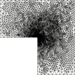
Figure 9: L-shaped goal-oriented Poisson problem with linear elements: On top left the initial mesh used to start all the adaptive strategies. From top middle to bottom right, the adaptive meshes obtained after seven iterations of refinement strategies steered by weighted estimators derived respectively from $\eta_{\mathrm{bw}}^{4,2}$, $\eta_{\mathrm{res}}$, $\eta_{\mathrm{bw}}^{\mathrm{b}}$ and $\eta_{\mathrm{zz}}$ for both primal and dual problems.

fig. 9 shows refined meshes after seven iterations of the weighted goal oriented method. We can see that the meshes are mainly refined in the re-entrant corner as well as in the region on the right top of it where the goal functional focuses. In fig. 10 we show the convergence curves of some of these adaptive strategies. For each strategy, $\eta_{u}=\eta_{z}$ is the estimator specified in the legend and $\eta_{w}=\eta_{u}\eta_{z}$. All the strategies we have tried led to very similar higher-order approximate errors. So for the sake of clarity we have replaced the approximate errors by an indicative line computed using a regression from the least squares method (lstsq error), leading to the line that fits the best the values of the different approximate errors. As we can see, these adaptive strategies are reaching an optimal convergence rate. Although it is also the case for all the other strategies we have tried, we do not show the other results for the sake of concision.

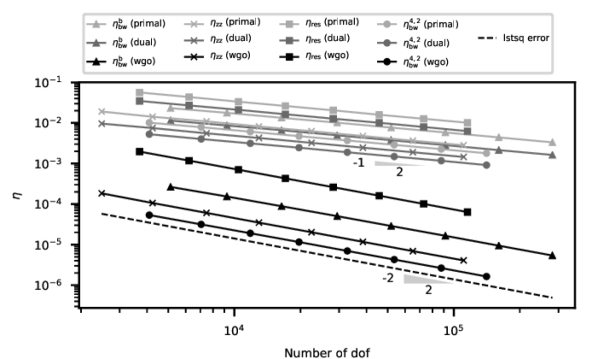
Figure 10: L-shaped goal-oriented Poisson problem with linear elements: plot comparing convergence of some goal-oriented adaptive strategies driven by four different estimators. Expected rates for primal and dual problems ($-0.5$) and goal functional ($-1$) shown by triangle markers. Comparison with an indicative line representing the higher order approximation of the errors of each strategy and obtained using least squares method.

In the left table of fig. 11 we show the efficiencies of the estimators $\eta_{w}$ where $\eta_{u}=\eta_{z}=\eta_{\mathrm{bw}}^{k_{+},k_{-}}$. On the right table of fig. 11 we take $\eta_{u}=\eta_{z}$ to be the estimators in the left column. As we can see on the efficiencies are not as good as in section 7.1. The two best estimators are those derived from $\eta_{\mathrm{bw}}^{4,0}$ and $\eta_{\mathrm{bw}}^{4,2}$. With $\eta_{\mathrm{bw}}^{3,0}$, they are the only cases where the goal-oriented estimator $\eta_{w}$ is performing better than the goal-oriented estimator derived from the Zienkiewicz–Zhu estimator. The estimators $\eta_{w}$ derived from the bubble Bank–Weiser estimator as well as from the residual estimator are poorly overestimating the error.

Figure 11: L-shaped goal-oriented Poisson problem with linear elements: efficiencies of the dual weighted estimators derived from $\eta_{\mathrm{bw}}^{k_{+},k_{-}}$ and other estimators on the last mesh of an adaptively refined hierarchy.

7.5 Nearly-incompressible elasticity

We consider the linear elasticity problem from [32] on the centered unit square domain $\Omega$ with homogeneous Dirichlet boundary conditions on $\Gamma_{D}=\Gamma$ ($u_{D}=0$). The first Lamé coefficient is set to $\mu=100$ and the Poisson ratio to $\nu=0.3$ and $\nu=0.499$. The problem data $\bm{f}$ is given by $\bm{f}=(f_{1},f_{2})$ with

$$\begin{array}[]{r c l}f_{1}(x,y)=-2\mu\pi^{3}\cos(\pi y)\sin(\pi y)\big{(}2\cos(2\pi x)-1\big{)},\\ f_{2}(x,y)=2\mu\pi^{3}\cos(\pi x)\sin(\pi x)\big{(}2\cos(2\pi y)-1\big{)}.\end{array}$$ (49)

The corresponding exact solution of the linear elasticity problem reads $\bm{u}=(u_{1},u_{2})$ with

$$u_{1}(x,y)=\pi\cos(\pi y)\sin^{2}(\pi x)\sin(\pi y),\ u_{2}(x,y)=-\pi\cos(\pi x)\sin(\pi x)\sin^{2}(\pi y),$$ (50)

the Herrmann pressure is zero everywhere on $\Omega$. In each case we discretize this problem using the Taylor–Hood element and an initial cartesian mesh and we apply our adaptive procedure driven by the Poisson estimator described in section 5.3.1. We compare the Poisson estimators derived from different Bank–Weiser estimators and the residual estimator.

As before, all the refinement strategies are achieving an optimal convergence rate no matter the value of $\nu$. fig. 12 shows the results for $\nu=0.3$. We notice that almost all the Poisson estimators derived from Bank–Weiser estimators have a very good efficiency. The best estimator in this case is $\eta_{\mathrm{bw}}^{2,0}$ closely followed by $\eta_{\mathrm{bw}}^{3,0}$, $\eta_{\mathrm{bw}}^{\mathrm{b}}$ and $\eta_{\mathrm{bw}}^{4,0}$. Although the residual estimator still performs the worst, it is sharper than in all the previous test cases. As we can notice on fig. 13, all the estimators are robust with respect to the incompressibility constraint. All the efficiencies have slightly increased and some estimators ($\eta_{\mathrm{bw}}^{2,0}$ and $\eta_{\mathrm{bw}}^{3,0}$) that where a lower bound of the error previously are now an upper bound.

Figure 12: Nearly-incompressible elasticity ($\nu=0.3$) problem with Taylor–Hood elements: efficiencies of the Poisson estimators derived from $\eta_{\mathrm{bw}}^{k_{+},k_{-}}$ and other estimators on the last mesh of an adaptively refined hierarchy.

Figure 13: Nearly-incompressible elasticity ($\nu=0.499$) problem with Taylor–Hood elements: efficiencies of the Poisson estimators derived from $\eta_{\mathrm{bw}}^{k_{+},k_{-}}$ and other estimators on the last mesh of an adaptively refined hierarchy.

7.6 Human femur modelled using linear elasticity

In this test case we consider a linear elasticity problem on a domain inspired by a human femur bone .

The goal of this test case is not to provide an accurate description of the behavior of the femur bone but to demonstrate the applicability of our implementation to 3D dimensional goal-oriented problem with large number of degrees of freedom: the linear elasticity problem to solve on the initial mesh, using Taylor-Hood element has 247,233 degrees of freedom while our last refinement step reaches 3,103,594 degrees of freedom.

The 3D mesh for analysis is build from the surface model using the C++ library CGAL [4] via the Python front-end pygalmesh. The material parameters, namely the Young’s modulus is set to $20$ GPa and the Poisson’s ratio to $0.42$ (see e.g. [69]). In addition, the load is given by $\mathbf{f}=(0,0,0)$, the Dirichlet data by $\bm{u}_{D}=0$ on $\Gamma_{D}\subsetneq\Gamma$ represented as the left dark gray region of the boundary in fig. 14 and $\bm{g}$ the traction data is defined as $\bm{g}=(0,0,0)$ on the center light gray region of the boundary and is constant on the right dark gray region of the boundary $\bm{g}=(-10^{-7},-10^{-7},10^{-6})$. The femur-shaped domain $\Omega$ as well as the initial and last meshes are shown in fig. 14. As we can see, the refinement occurs mainly in the central region of the femur, where the goal functional $J$ focus. Some artefacts can be seen as stains of refinement in the central region due to the fact that we use the initial mesh as our geometry and on the left due to the discontinuity in the boundary conditions.

In fig. 15 the primal solution is given by the couple $(\mathbf{u}_{2},p_{1})$ and the dual solution by $(\mathbf{z}_{2},\kappa_{1})$. As we can notice and as expected, the weighted estimator $\eta_{w}$ converges twice as fast as the primal and dual estimators.

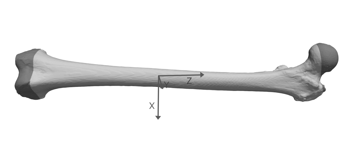
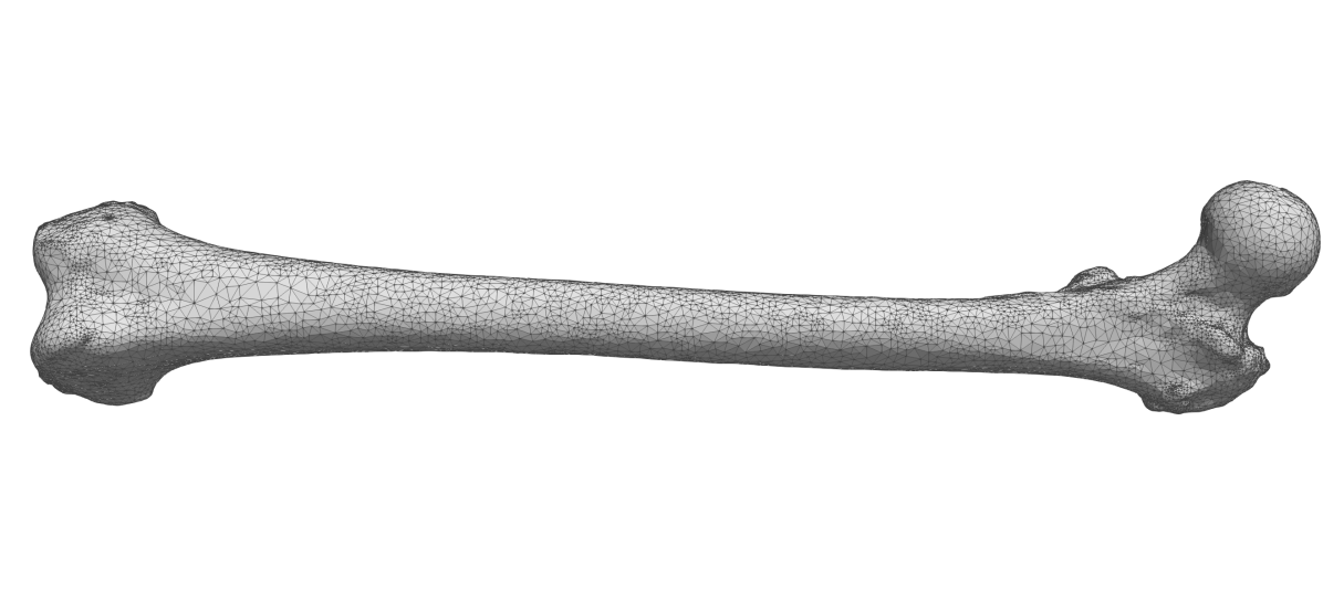
Figure 14: Femur bone linear elasticity problem with Taylor–Hood elements: on the top, the three different regions of the boundary corresponding to different boundary conditions: the left dark grey region is the non-zero Neumann boundary, the middle light grey region is the zero Neumann boundary and the right dark grey region is the Dirichlet boundary. In the middle, the initial mesh. On the bottom, the last mesh after several steps of adaptive refinement.

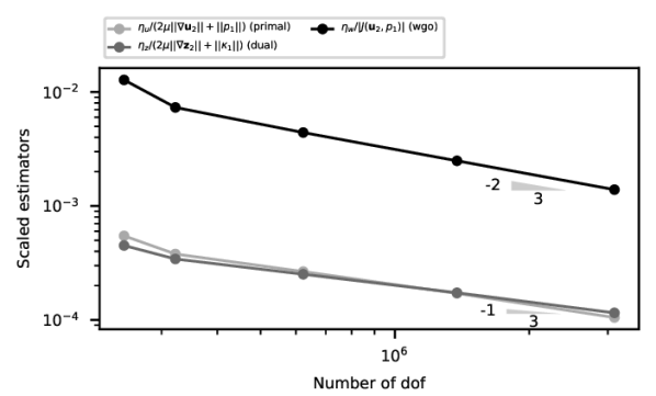
Figure 15: Femur bone linear elasticity problem with Taylor–Hood elements: convergence curves of the primal, dual and weighted estimators respectively scaled by the norm of the primal solution, dual solution and magnitude of the goal functional evaluated in the primal solution.

7.7 Strong scaling study

Finally, we provide results showing that our implementation scales strongly in parallel and that for a large-scale three-dimensional problem this error estimation takes significantly less time than the solution of the primal problem. In this section we use the new DOLFINx solver [44] with the matching implementation of our algorithm.

We briefly discuss some aspects that are important for interpretation of the results. For a given cell the computation of the Bank–Weiser estimator requires geometry and solution data on the current cell and on all cells attached across its facets. So in a parallel computing context, cells located on the boundary of a partition require data from cells owned by another process. Both DOLFIN and DOLFINx support facet–mode ghosting where all data owned by cells on a partition boundary that share a facet are duplicated by the other process (ghost data). After the solution of the primal linear system the ghost data is updated between processes, which requires parallel communication. After this update, each process has a local copy of all of the data from the other rank needed to compute the Bank–Weiser estimator, and so the computation of the estimator is entirely local to a rank, i.e. without further parallel communication.

Because of this locality a proper implementation of this algorithm should demonstrate strong scaling performance. Furthermore, it would be desirable that the error estimation takes significantly less time than the solution of the primal problem even when using state-of-the art linear solution strategies. The results in this section demonstrate that this is indeed the case.

We solve eq. 1 where $\Omega$ is the unit cube $[0,1]^{3}$, $\Gamma_{D}=\partial\Omega$ and $\Gamma_{N}=\varnothing$. The data of this problem are given by $f(x,y,z)=12\pi^{2}\sin(2\pi x)\sin(2\pi y)\sin(2\pi z)$ and $u_{D}(x,y,z)=0$. Given these data the solution $u$ of eq. 1 is given by $u(x,y,z)=\sin(2\pi x)\sin(2\pi y)\sin(2\pi z)$. We use continuous quadratic Lagrange finite elements and the Bank–Weiser error estimation is performed using the pair $V_{T}^{3}$/$V_{T}^{2}$. The primal linear system matrix and right-hand side vector are assembled using standard routines in DOLFINx. The resulting linear system is solved with PETSc [14] using the conjugate gradient method preconditioned with Hypre BoomerAMG algebraic multigrid [38].

The strong scaling study was carried out on the Aion cluster within the HPC facilities of the University of Luxembourg [72]. The Aion cluster is a Atos/Bull/AMD supercomputer composed of 318 compute nodes each containing two AMD Epyc ROME 7H12 processors with 64 cores per processor (128 cores per node). The nodes are connected through a Fast InfiniBand (IB) HDR 100Gbps interconnect in a ‘fat-tree’ topology. We invoke jobs using SLURM and ask for a contiguous allocation of nodes and exclusivity (no competing jobs) on each node. DOLFINx and PETSc are built using GCC 10.2.0 with Intel MPI and OpenBLAS. We use DOLFINx through its Python interface. The problem size is kept fixed at around 135 million degrees of freedom and the number of MPI ranks is increased from 128 (1 node, no interconnect communication) through to 2048 (16 nodes, interconnect communication) by doubling the number of nodes and ranks used in the previous computation.

In fig. 16 we show the results of the strong scaling study. We show wall time against MPI ranks and dof per rank for the primal linear system assembly, primal linear system solve, and the error estimation. For error estimation we are measuring steps 2 through 5 of section 4.1. Both the solve and estimation scale almost perfectly down to around 65 thousand dofs per rank. The primal system assembly does not scale as well as the estimation. This is because the primal system assembly is constrained by communication overheads and memory bandwidth, whereas the Bank–Weiser estimator computation is fully local and has much higher arithmetic intensity, so has not yet hit bandwidth limits of our system on the largest run. A further study (results not shown) using 96 MPI ranks per node yielded lower wall times and better strong scaling for primal linear system assembly, but the overall time for estimation and linear system solve increased and dominated any gains made in assembly. Comparing linear system assembly and solve with estimation time we can see that estimation is approximately one order of magnitude faster than solve time.

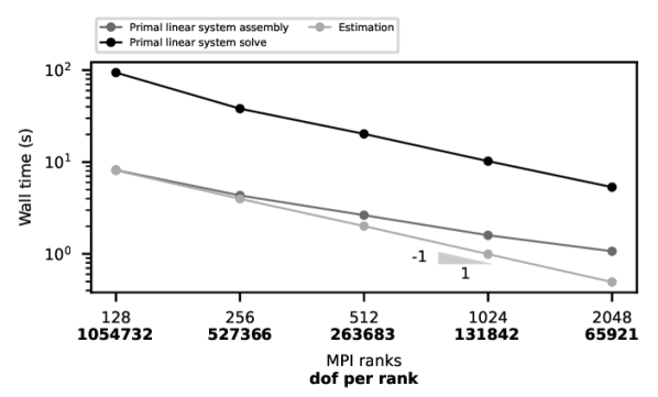
Figure 16: Strong scaling study on the University of Luxmebourg Aion HPC. Wall times for primal linear system assembly, primal linear system solve and error estimation of a three-dimensional Poisson finite element problem on the unit square, discretized with quadratic elements. $1/1$ triangle represents ideal strong scaling.

8 Conclusions

In this paper we have shown how the error estimator of Bank–Weiser, involving the solution of a local problem on a special finite element space, can be mathematically reformulated and implemented straightforwardly in a modern finite element software with the aid of automatic code generation techniques. Through a series of numerical results we have shown that the estimator is highly competitive in accurately predicting the total global error and in driving an adaptive mesh refinement strategy. Furthermore, the basic methodology and implementation for the Poisson problem can be extended to tackle more complex mixed discretizations of PDEs including nearly-incompressible elasticity or Stokes problems. We have also shown the (strong) scalability of our method when implemented in parallel and that the error estimation time is significantly lower than the primal solution time on a large problem.

Acknowledgements

The three-dimensional problems presented in this paper were carried out using the HPC facilities of the University of Luxembourg [72].

We would like to thank Nathan Sime and Chris Richardson for helpful discussions on FEniCS’s discontinuous Galerkin discretizations and PLAZA refinement strategy, respectively. We would also like to thank Prof. Roland Becker for the motivating and fruitful discussions.

Supplementary material

The DOLFINx version of the code can be found at https://github.com/jhale/fenicsx-error-estimation and the DOLFIN version at https://github.com/rbulle/fenics-error-estimation.

The appendices 1 and 2 in of supplementary material contain two snippets showing the implementation of the Poisson estimator and the Poisson estimator for the nearly-incompressible elasticity problem using the DOLFIN version of the code. A simplified version of the code (LGPLv3) used to produce the results in this paper is archived at https://doi.org/10.6084/m9.figshare.10732421. A Docker image [46] is provided in which this code can be executed.

Appendices

A The residual estimator

A.1 Poisson equation

The class of residual estimators, the explicit residual estimator is part of, have been introduced for the first time in [13]. Let $h_{T}$ be the diameter (see e.g. [70]) of the cell $T$ and $h_{E}$ be the diameter of the facet $E$. The explicit residual estimator [3] on a cell $T$ for the Poisson problems eqs. 2 and 4 is defined as

$$\eta_{\mathrm{res},T}^{2}:=h_{T}^{2}\lVert f_{T}+\Delta u_{k}\rVert_{T}^{2}+\sum_{E\in\mathcal{E}_{I}\cap\partial T}\frac{1}{2}h_{E}\lVert\left[\![\partial_{n}u_{k}\right]\!]_{E}\rVert^{2}_{E}+\sum_{E\in\mathcal{E}_{N}\cap\partial T}h_{E}\lVert g_{E}-\partial_{n}u_{k}\rVert^{2}_{E},$$ (1)

where $f_{h}$ and $g_{h}$ are the $L^{2}$ projections of $f$ and $g$ on $V^{k}$ respectively. In order to take into account inhomogeneous Dirichlet boundary conditions, we define in addition the Dirichlet oscillations. If $E:=\Gamma_{D}\cap T\neq\varnothing$, then

$$\mathrm{osc}_{D,E}^{2}:=h_{E}\lVert\nabla_{\Gamma}\left(g_{E}-u_{k}\right)\rVert^{2}_{L^{2}(E)},$$ (2)

where $\nabla_{\Gamma}$ is the surface gradient and $g_{E}:=\pi^{+}_{T}(g)$ is the $L^{2}$ projection of $g$ onto $V^{k+1}_{T}$ [11]. The global residual estimator reads

$$\eta_{\mathrm{res}}^{2}:=\sum_{T\in\mathcal{T}}\eta_{\mathrm{res},T}^{2}+\mathrm{osc}_{D,\overline{T}\cap\Gamma_{D}}^{2}.$$ (3)

A.2 Linear elasticity equations

The residual estimator for the linear elasticity problem eqs. 41a, 41b, 43a and 43b is given by

$$\eta_{\mathrm{res},T}^{2}:=\rho_{T}\lVert\bm{R}_{T}\rVert_{T}^{2}+\rho_{d}\lVert r_{T}\rVert_{T}^{2}+\sum_{E\in\partial T}\rho_{E}\lVert\bm{R}_{E}\rVert_{E}^{2},$$ (4)

where the residuals $\bm{R}_{T}$, $r_{T}$ and $\bm{R}_{E}$ are respectively defined in eqs. 44a, 44b and 44c and the constants $\rho_{T}$, $\rho_{d}$ and $\rho_{E}$ are given by

$$\rho_{T}:=\frac{h_{T}(2\mu)^{-1/2}}{2},\quad\rho_{d}:=\big{(}\lambda^{-1}+(2\mu)^{-1}\big{)}^{-1},\quad\rho_{E}:=\frac{h_{E}(2\mu)^{-1}}{2},$$ (5)

with $h_{T}$ the diameter of the cell $T$ and $h_{E}$ the length of the edge $E$. The global estimator reads

$$\eta_{\mathrm{res}}^{2}:=\sum_{T\in\mathcal{T}}\eta_{\mathrm{res},T}^{2}.$$ (6)

B The Zienkiewicz–Zhu estimator

The Zienkiewicz–Zhu estimator is a gradient recovery estimator based on an averaging technique introduced in [76]. This estimator belongs to a general class of recovery estimators, see [27, 28, 75] for recent surveys and a reformulation of the recovery procedure in an $H(\mathrm{div})$-conforming space that has superior performance for problems with sharp interfaces. Despite the fact that some recovery estimators, especially when based on least squares fitting, are available for higher order finite elements (see for example [77]) we only consider the original estimator, defined for a piecewise linear finite element framework.

Given the finite element solution $u_{1}\in V^{1}$ the numerical flux $\rho_{1}:=\nabla u_{1}$ is a piecewise constant vector field. For each vertex $\chi\in\mathcal{N}$ in the mesh we denote $\omega_{\chi}$ the domain covered by the union of cells $T$ having common vertex $\chi$. The recovered flux $G(\rho_{1})\in[V^{1}]^{2}$ has values at the degrees of freedom associated with the vertices $\mathcal{N}$ given by

$$G(\rho_{1})(\chi):=\frac{1}{|\omega_{\chi}|}\int_{\omega_{\chi}}\rho_{1}\text{ d$x$},\quad\forall\chi\in\mathcal{N}.$$ (7)

The local Zienkiewicz–Zhu estimator is then defined as the discrepancy between the recovered flux and the numerical flux

$$\eta_{\mathrm{zz},T}:=\lVert G(\rho_{1})-\rho_{1}\rVert_{T},\quad\forall T\in\mathcal{T}.$$ (8)

As for the residual estimator, we add Dirichlet oscillations (see eq. 2) to take into account the Dirichlet boundary error. The global Zienkiewicz–Zhu estimator is given by

$$\eta_{\mathrm{zz}}^{2}:=\sum_{T\in\mathcal{T}}\eta_{\mathrm{zz},T}^{2}+\mathrm{osc}_{D,\overline{T}\cap\Gamma_{D}}^{2}.$$ (9)

The code in the supplementary material contains a prototype implementation of the Zienkiewicz–Zhu estimator in FEniCS. We have implemented the local recovered flux calculation in Python rather than C++, so the runtime performance is far from optimal.

References

- [1] Mark Ainsworth. The influence and selection of subspaces for a posteriori error estimators. Numerische Mathematik, 73(4):399–418, June 1996.
- [2] Mark Ainsworth and J. Tinsley Oden. A Posteriori Error Estimators for the Stokes and Oseen Equations. SIAM Journal on Numerical Analysis, 34(1):228–245, February 1997.
- [3] Mark Ainsworth and J. Tinsley Oden. A Posteriori Error Estimation in Finite Element Analysis. 2011.
- [4] Pierre Alliez, Clément Jamin, Laurent Rineau, Stéphane Tayeb, Jane Tournois, and Mariette Yvinec. 3D mesh generation. In CGAL User and Reference Manual. CGAL Editorial Board, 5.1 edition, 2020.
- [5] Martin Alnæs, Jan Blechta, Johan Hake, August Johansson, Benjamin Kehlet, Anders Logg, Chris Richardson, Johannes Ring, Marie E Rognes, and Garth N Wells. The FEniCS Project Version 1.5. Archive of Numerical Software, Vol 3, 2015.
- [6] Martin S. Alnæs, Anders Logg, Kristian B. Ølgaard, Marie E. Rognes, and Garth N. Wells. Unified form language: A domain-specific language for weak formulations of partial differential equations. ACM Transactions on Mathematical Software, 40(2):1–37, February 2014.
- [7] Patrick R. Amestoy, Iain S. Duff, Jean-Yves L’Excellent, and Jacko Koster. A Fully Asynchronous Multifrontal Solver Using Distributed Dynamic Scheduling. SIAM Journal on Matrix Analysis and Applications, 23(1):15–41, January 2001.
- [8] Patrick R. Amestoy, Abdou Guermouche, Jean-Yves L’Excellent, and Stéphane Pralet. Hybrid scheduling for the parallel solution of linear systems. Parallel Computing, 32(2):136–156, February 2006.
- [9] A. Anciaux-Sedrakian, L. Grigori, Z. Jorti, J. Papež, and S. Yousef. Adaptive solution of linear systems of equations based on a posteriori error estimators. Numer. Algorithms, 84(1):331–364, 2020.
- [10] Mario Arioli, Jörg Liesen, Agnieszka Miçdlar, and Zdeněk Strakoš. Interplay between discretization and algebraic computation in adaptive numerical solutionof elliptic PDE problems. GAMM-Mitteilungen, 36(1):102–129, aug 2013.
- [11] M. Aurada, M. Feischl, J. Kemetmüller, M. Page, and D. Praetorius. Each H 1/2 –stable projection yields convergence and quasi–optimality of adaptive FEM with inhomogeneous Dirichlet data in R d. ESAIM Math. Model. Numer. Anal., 47(4):1207–1235, jul 2013.
- [12] I. Babuska and M. Vogelius. Feedback and adaptive finite element solution of one-dimensional boundary value problems. Numerische Mathematik, 44(1):75–102, February 1984.
- [13] I. Babuška and W. C. Rheinboldt. A-posteriori error estimates for the finite element method. International Journal for Numerical Methods in Engineering, 12(10):1597–1615, 1978.
- [14] Satish Balay, Shrirang Abhyankar, Mark F Adams, Jed Brown, Peter Brune, Kris Buschelman, Lisandro Dalcin, Victor Eijkhout, William D Gropp, Dinesh Kaushik, Matthew G Knepley, Lois Curfman McInnes, Karl Rupp, Barry F Smith, Stefano Zampini, Hong Zhang, and Hong Zhang. PETSc Users Manual. Technical Report ANL-95/11 - Revision 3.7, Argonne National Laboratory, 2016.
- [15] R. E. Bank and A. Weiser. Some a posteriori error estimators for elliptic partial differential equations. Mathematics of Computation, 44(170):283–283, May 1985.
- [16] Randolph E. Bank. PLTMG: A Software Package for Solving Elliptic Partial Differential Equations: Users’ Guide 8.0. Society for Industrial and Applied Mathematics, January 1998.
- [17] Randolph E Bank, Jinchao Xu, and Bin Zheng. Superconvergent Derivative Recovery for Lagrange Triangular Elements of Degree p on Unstructured Grids. SIAM J. Numer. Anal., 45(5):2032–2046, 2007.
- [18] S. Bartels, C. Carstensen, and G. Dolzmann. Inhomogeneous Dirichlet conditions in a priori and a posteriori finite element error analysis. Numerische Mathematik, 99(1):1–24, November 2004.
- [19] Sören Bartels and Carsten Carstensen. Each averaging technique yields reliable a posteriori error control in FEM on unstructured grids. Part II: Higher order FEM. Mathematics of Computation, 71(239):971–994, February 2002.
- [20] Roland Becker, Elodie Estecahandy, and David Trujillo. Weighted Marking for Goal-oriented Adaptive Finite Element Methods. SIAM Journal on Numerical Analysis, 49(6):2451–2469, January 2011.
- [21] Roland Becker and Rolf Rannacher. An optimal control approach to a posteriori error estimation in finite element methods. Acta Numer., 10:1–102, 2001.
- [22] L. Beirão da Veiga, C. Chinosi, C. Lovadina, and R. Stenberg. A-priori and a-posteriori error analysis for a family of Reissner–Mindlin plate elements. BIT Numerical Mathematics, 48(2):189–213, June 2008.
- [23] Alex Bespalov, Dirk Praetorius, Leonardo Rocchi, and Michele Ruggeri. Goal-oriented error estimation and adaptivity for elliptic PDEs with parametric or uncertain inputs. Computer Methods in Applied Mechanics and Engineering, 345:951–982, March 2019.
- [24] Alex Bespalov, Leonardo Rocchi, and David Silvester. T-IFISS: a toolbox for adaptive FEM computation. Computers & Mathematics with Applications, 2020.
- [25] Raphaël Bulle, Franz Chouly, Jack S. Hale, and Alexei Lozinski. Removing the saturation assumption in Bank–Weiser error estimator analysis in dimension three. Applied Mathematics Letters, 107:106429, September 2020.
- [26] Raphaël Bulle and Jack S Hale. An implementation of the Bank-Weiser error estimator in the FEniCS Project finite element software. December 2020.
- [27] Zhiqiang Cai, Cuiyu He, and Shun Zhang. Improved ZZ a posteriori error estimators for diffusion problems: Conforming linear elements. Computer Methods in Applied Mechanics and Engineering, 313:433–449, January 2017.
- [28] Zhiqiang Cai and Shun Zhang. Recovery-Based Error Estimator for Interface Problems: Conforming Linear Elements. SIAM Journal on Numerical Analysis, 47(3):2132–2156, January 2009.
- [29] C. Carstensen, M. Feischl, M. Page, and D. Praetorius. Axioms of adaptivity. Computers & Mathematics with Applications, 67(6):1195–1253, April 2014.
- [30] C. Carstensen and C. Merdon. Estimator Competition for Poisson Problems. Journal of Computational Mathematics, 28, 2010.
- [31] Carsten Carstensen and Sören Bartels. Each averaging technique yields reliable a posteriori error control in FEM on unstructured grids. Part I: Low order conforming, nonconforming, and mixed FEM. Mathematics of Computation, 71(239):945–969, February 2002.
- [32] Carsten Carstensen and Joscha Gedicke. Robust residual-based a posteriori Arnold–Winther mixed finite element analysis in elasticity. Computer Methods in Applied Mechanics and Engineering, 300:245–264, March 2016.
- [33] Concha INRIA Project-Team. Complex Flow Simulation Codes based on High-order and Adaptive methods.
- [34] Michel Duprez, Stéphane Pierre Alain Bordas, Marek Bucki, Huu Phuoc Bui, Franz Chouly, Vanessa Lleras, Claudio Lobos, Alexei Lozinski, Pierre-Yves Rohan, and Satyendra Tomar. Quantifying discretization errors for soft tissue simulation in computer assisted surgery: A preliminary study. Applied Mathematical Modelling, 77:709–723, January 2020.
- [35] Willy Dörfler. A Convergent Adaptive Algorithm for Poisson’s Equation. SIAM Journal on Numerical Analysis, 33(3):1106–1124, June 1996.
- [36] Willy Dörfler and Ricardo H. Nochetto. Small data oscillation implies the saturation assumption. Numerische Mathematik, 91(1):1–12, March 2002.
- [37] Howard C. Elman, Alison Ramage, and David J. Silvester. IFISS: A Computational Laboratory for Investigating Incompressible Flow Problems. SIAM Review, 56(2):261–273, January 2014.
- [38] Robert D Falgout and Ulrike Meier Yang. hypre: A Library of High Performance Preconditioners. In Peter M A Sloot, Alfons G Hoekstra, C J Kenneth Tan, and Jack J Dongarra, editors, Comput. Science — ICCS 2002, number 2331 in Lecture Notes in Computer Science, pages 632–641. Springer Berlin Heidelberg, apr 2002.
- [39] Stefan Funken, Dirk Praetorius, and Philipp Wissgott. Efficient implementation of adaptive P1-FEM in Matlab. Computational Methods in Applied Mathematics, 11(4):460–490, 2011.
- [40] Thomas H Gibson, Lawrence Mitchell, David A Ham, and Colin J Cotter. Slate: extending Firedrake’s domain-specific abstraction to hybridized solvers for geoscience and beyond. Geosci. Model Dev. Discuss., pages 1–40, apr 2019.
- [41] Michael B. Giles and Endre Süli. Adjoint methods for PDEs: a posteriori error analysis and postprocessing by duality. Acta Numerica, 11:145–236, January 2002.
- [42] P Grisvard. Elliptic problems in nonsmooth domains, volume 24 of Monographs and Studies in Mathematics. Pitman (Advanced Publishing Program), Boston, MA, 1985.
- [43] Gaël Guennebaud, Benoît Jacob, and Others. Eigen v3. 2010.
- [44] Michal Habera, Jack S. Hale, Chris Richardson, Johannes Ring, Marie Rognes, Nate Sime, and Garth N. Wells. FEniCSX: A sustainable future for the FEniCS Project. 2 2020.
- [45] Jack S. Hale, Matteo Brunetti, Stéphane P.A. Bordas, and Corrado Maurini. Simple and extensible plate and shell finite element models through automatic code generation tools. Computers & Structures, 209:163–181, October 2018.
- [46] Jack S. Hale, Lizao Li, Christopher N. Richardson, and Garth N. Wells. Containers for Portable, Productive, and Performant Scientific Computing. Computing in Science & Engineering, 19(6):40–50, November 2017.
- [47] Frédéric Hecht. New development in freefem++. J. Numer. Math., 20(3-4):1–14, jan 2012.
- [48] C. A. R. Hoare. Algorithm 65: find. Communications of the ACM, 4(7):321–322, July 1961.
- [49] P. Houston, B. Senior, and E. Süli. Sobolev regularity estimation for hp-adaptive finite element methods. In Numer. Math. Adv. Appl., pages 631–656. Springer Milan, Milano, 2003.
- [50] Paul Houston and Nathan Sime. Automatic Symbolic Computation for Discontinuous Galerkin Finite Element Methods. SIAM Journal on Scientific Computing, 40(3):C327–C357, January 2018.
- [51] Arbaz Khan, Catherine E. Powell, and David J. Silvester. Robust a posteriori error estimators for mixed approximation of nearly incompressible elasticity. International Journal for Numerical Methods in Engineering, 119(1):18–37, July 2019.
- [52] Robert C. Kirby. Algorithm 839: FIAT, a new paradigm for computing finite element basis functions. ACM Transactions on Mathematical Software, 30(4):502–516, December 2004.
- [53] Robert C. Kirby and Anders Logg. A compiler for variational forms. ACM Transactions on Mathematical Software, 32(3):417–444, September 2006.
- [54] Qifeng Liao and David Silvester. A simple yet effective a posteriori estimator for classical mixed approximation of Stokes equations. Applied Numerical Mathematics, 62(9):1242–1256, September 2012.
- [55] Anders Logg and Garth N. Wells. DOLFIN: Automated finite element computing. ACM Transactions on Mathematical Software, 37(2):1–28, April 2010.
- [56] William F. Mitchell. A collection of 2D elliptic problems for testing adaptive grid refinement algorithms. Appl. Math. Comput., 220(February):350–364, sep 2013.
- [57] William F. Mitchell. A collection of 2D elliptic problems for testing adaptive grid refinement algorithms. Applied Mathematics and Computation, 220:350–364, September 2013.
- [58] Mario S. Mommer and Rob Stevenson. A Goal-Oriented Adaptive Finite Element Method with Convergence Rates. SIAM Journal on Numerical Analysis, 47(2):861–886, January 2009.
- [59] Ricardo H. Nochetto. Removing the saturation assumption in a posteriori error analysis. Istit. Lomb. Accad. Sci. Lett. Rend. A, 127(1):67–82 (1994), 1993.
- [60] Ricardo H Nochetto, Kunibert G Siebert, and Andreas Veeser. Theory of adaptive finite element methods: An introduction. In Ronald DeVore and Angela Kunoth, editors, Multiscale, Nonlinear Adapt. Approx., pages 409–542, Berlin, Heidelberg, 2009. Springer Berlin Heidelberg.
- [61] J. Papež, Z. Strakoš, and M. Vohralík. Estimating and localizing the algebraic and total numerical errors using flux reconstructions. Numer. Math., 138(3):681–721, mar 2018.
- [62] Carl-Martin Pfeiler and Dirk Praetorius. Dörfler marking with minimal cardinality is a linear complexity problem. arXiv1907.13078 [cs, math], July 2019.
- [63] A. Plaza and G.F. Carey. Local refinement of simplicial grids based on the skeleton. Applied Numerical Mathematics, 32(2):195–218, February 2000.
- [64] Christophe Prud’homme, Vincent Chabannes, Vincent Doyeux, Mourad Ismail, Abdoulaye Samake, and Goncalo Pena. Feel++ : A computational framework for Galerkin Methods and Advanced Numerical Methods. ESAIM: Proceedings, 38:429–455, December 2012.
- [65] Florian Rathgeber, David A. Ham, Lawrence Mitchell, Michael Lange, Fabio Luporini, Andrew T. T. Mcrae, Gheorghe-Teodor Bercea, Graham R. Markall, and Paul H. J. Kelly. Firedrake: Automating the Finite Element Method by Composing Abstractions. ACM Transactions on Mathematical Software, 43(3):1–27, January 2017.
- [66] Yves Renard and K Poulios. GetFEM: Automated FE modeling of multiphysics problems based on a generic weak form language. (Submitted), 2020.
- [67] Rodolfo Rodríguez. Some remarks on Zienkiewicz-Zhu estimator. Numerical Methods for Partial Differential Equations, 10(5):625–635, September 1994.
- [68] Marie E. Rognes and Anders Logg. Automated Goal-Oriented Error Control I: Stationary Variational Problems. SIAM Journal on Scientific Computing, 35(3):C173–C193, January 2013.
- [69] Fabienne Rupin, Amena Saied, Davy Dalmas, Françoise Peyrin, Sylvain Haupert, Etienne Barthel, Georges Boivin, and Pascal Laugier. Experimental determination of Young modulus and Poisson ratio in cortical bone tissue using high resolution scanning acoustic microscopy and nanoindentation. J. Acoust. Soc. Am., 123(5):3785–3785, May 2008.
- [70] L. Ridgway Scott and Shangyou Zhang. Finite element interpolation of nonsmooth functions satisfying boundary conditions. Mathematics of Computation, 54(190):483–483, May 1990.
- [71] Stéfan van der Walt, S Chris Colbert, and Gaël Varoquaux. The NumPy Array: A Structure for Efficient Numerical Computation. Computing in Science & Engineering, 13(2):22–30, March 2011.
- [72] Sebastien Varrette, Pascal Bouvry, Hyacinthe Cartiaux, and Fotis Georgatos. Management of an academic HPC cluster: The UL experience. In 2014 International Conference on High Performance Computing & Simulation (HPCS), pages 959–967, Bologna, Italy, July 2014. IEEE.
- [73] R. Verfürth. A posteriori error estimation and adaptive mesh-refinement techniques. Journal of Computational and Applied Mathematics, 50(1-3):67–83, May 1994.
- [74] Pauli Virtanen, Ralf Gommers, Travis E. Oliphant, Matt Haberland, Tyler Reddy, David Cournapeau, Evgeni Burovski, Pearu Peterson, Warren Weckesser, Jonathan Bright, Stéfan J. van der Walt, Matthew Brett, Joshua Wilson, K. Jarrod Millman, Nikolay Mayorov, Andrew R. J. Nelson, Eric Jones, Robert Kern, Eric Larson, C. J. Carey, Ilhan Polat, Yu Feng, Eric W. Moore, Jake VanderPlas, Denis Laxalde, Josef Perktold, Robert Cimrman, Ian Henriksen, E. A. Quintero, Charles R. Harris, Anne M. Archibald, Antônio H. Ribeiro, Fabian Pedregosa, Paul van Mulbregt, and Contributors. SciPy 1.0–Fundamental Algorithms for Scientific Computing in Python. Nature Methods, 17(3):261–272, March 2020.
- [75] Zhimin Zhang and Ningning Yan. Recovery type a posteriori error estimates in finite element methods. J. Appl. Math. Comput., 8(2):235–251, 2001.
- [76] O. C. Zienkiewicz and J. Z. Zhu. A simple error estimator and adaptive procedure for practical engineering analysis. International Journal for Numerical Methods in Engineering, 24(2):337–357, February 1987.
- [77] O. C. Zienkiewicz and J. Z. Zhu. The superconvergent patch recovery (SPR) and adaptive finite element refinement. Computer Methods in Applied Mechanics and Engineering, 101(1):207–224, December 1992.
- [78] Kristian B. Ølgaard, Anders Logg, and Garth N. Wells. Automated Code Generation for Discontinuous Galerkin Methods. SIAM Journal on Scientific Computing, 31(2):849–864, January 2009.