Axisymmetric dynamo action
produced by differential rotation,
with anisotropic electrical conductivity
and anisotropic magnetic permeability

Abstract

The effect on dynamo action of an anisotropic electrical conductivity conjugated to an anisotropic magnetic permeability is considered. Not only is the dynamo fully axisymmetric, but it requires only a simple differential rotation, which twice challenges the well-established dynamo theory. Stability analysis is conducted entirely analytically, leading to an explicit expression of the dynamo threshold. The results show a competition between the anisotropy of electrical conductivity and that of magnetic permeability, the dynamo effect becoming impossible if the two anisotropies are identical. For isotropic electrical conductivity, Cowling’s neutral point argument does imply the absence of an azimuthal component of current density, but does not prevent the dynamo effect as long as the magnetic permeability is anisotropic.

1 Introduction

The dynamo effect is a magnetic instability produced by the displacement of an electrically conducting medium, without the aid of a magnet or a remanent magnetic field. A part of the kinetic energy of the moving medium is thus transferred into magnetic energy. This process is the most likely candidate to explain the ubiquity of magnetic fields observed in astrophysical objects (Rincon, 2019). The increasing resolution of numerical simulations of dynamo equations makes it possible to reproduce, ever better, the magnetic features measured in natural objects (Schaeffer et al., 2017). Experiments have also successfully demonstrated the possibility of dynamo action (Gailitis et al., 2001; Stieglitz & Müller, 2001; Monchaux et al., 2007), although it remains difficult to replicate in the laboratory processes occurring on a geophysical or astrophysical scale (Alboussière et al., 2011; Tigrine et al., 2019). This is why, since the very first dynamo experiments (Lowes & Wilkinson, 1963, 1968), the use of materials with the highest product of electrical conductivity and magnetic permeability, has been favoured. In most cases it led to the choice of solid iron alloys (high permeability) or liquid sodium (high conductivity) for the moving parts. In the VKS experiment, in which liquid sodium was driven by impellers, the high magnetic permeability of the impellers was revealed to be crucial to achieve a dynamo effect (Miralles et al., 2013; Kreuzahler et al., 2017; Nore et al., 2018). The choice of materials for the static parts, like the walls of the container, has also been proved to be crucial in relation to the electromagnetic boundary conditions (Avalos-Zuñiga et al., 2003; Avalos-Zuñiga & Plunian, 2005), leading for example to the use of copper walls (Monchaux et al., 2007).

The role in the dynamo effect of an anisotropic electrical conductivity has been studied for different geometries: Cartesian (Ruderman & Ruzmaikin, 1984; Alboussière et al., 2020), cylindrical (Plunian & Alboussière, 2020) and toroidal (Lortz, 1989). Although at first glance it is difficult to imagine such an anisotropic electrical conductivity in natural objects, it is far from impossible. For example, in a plasma subjected to a magnetic field, it is known that the electrical conductivity in the direction parallel to the magnetic field is twice that in the direction perpendicular to the magnetic field (Braginskii, 1965). In the case of the Earth, seismic observations provide strong evidence that the elastic response of the solid inner core is anisotropic. This is most likely due to the alignment of hexagonal close-packed iron crystals, occurring during the solidification of the inner core (Deuss, 2014). Incidentally it has been shown that, in hexagonal close-packed iron, the thermal conductivity and the electrical conductivity, which are directly related, are anisotropic (Ohta et al., 2018). Eventually, this suggests that the electrical conductivity of the inner core is anisotropic. Finally, in a turbulent electrically conducting fluid, the interaction between the small scales of the velocity field and those of the magnetic field can generate a large-scale magnetic field by dynamo action. Such a process can be modeled using the so-called mean-field approach (Krause & Rädler, 1980), possibly leading to a large-scale anisotropic electrical conductivity (Brandenburg, 2018).

From a theoretical point of view, an interesting consequence of considering an anisotropic conductivity is the possibility of obtaining an axisymmetric dynamo effect (Plunian & Alboussière, 2020), allowing one to bypass the well-known Cowling’s antidynamo theorem (Cowling, 1934; Kaiser & Tilgner, 2014). Indeed, if it is anisotropic, then the electrical conductivity becomes a tensor, instead of being a scalar, which defeats Cowling’s neutral point argument. In addition, the use of an anisotropic conductivity leads to dynamo action for a motion as simple as shear (Ruderman & Ruzmaikin, 1984; Alboussière et al., 2020; Plunian & Alboussière, 2020), which is otherwise impossible to achieve.

Here we investigate the role of an anisotropic electrical conductivity conjugated to an anisotropic magnetic permeability. An anisotropic magnetic permeability is not expected in natural objects. However, as explained above, this may be of interest for dynamo experiments, in order to reduce the dynamo threshold. In contrast to previous dynamo studies (Busse & Wicht, 1992; Kaiser & Tilgner, 1999), here the electrical conductivity and magnetic permeability do not depend on time or space coordinates. In addition, they are stationary and axisymmetric.

2 Conductivity and permeability anisotropy

We consider a material such that the electrical conductivity and magnetic permeability are denoted $\sigma^{\parallel}$ and $\mu^{\parallel}$ in a given direction q, and $\sigma^{\perp}$ and $\mu^{\perp}$ in the directions perpendicular to q.

Writing Ohm’s law, ${\bf J}=\sigma^{\parallel}{\bf E}$ in the direction of q and ${\bf J}=\sigma^{\perp}{\bf E}$ in the directions perpendicular to q, leads to the following conductivity tensor:

$$[\sigma_{ij}]=\sigma^{\perp}\delta_{ij}+(\sigma^{\parallel}-\sigma^{\perp})q_{i}q_{j}.$$ (1)

Inverting (1) leads to the resistivity tensor: (Ruderman & Ruzmaikin, 1984)

$$[\sigma_{ij}]^{-1}=\frac{1}{\sigma^{\perp}}\delta_{ij}+(\frac{1}{\sigma^{\parallel}}-\frac{1}{\sigma^{\perp}})q_{i}q_{j}.$$ (2)

Similarly, a magnetic permeability tensor can be defined as

$$[\mu_{ij}]=\mu^{\perp}\delta_{ij}+(\mu^{\parallel}-\mu^{\perp})q_{i}q_{j},$$ (3)

with the inverse tensor

$$[\mu_{ij}]^{-1}=\frac{1}{\mu^{\perp}}\delta_{ij}+(\frac{1}{\mu^{\parallel}}-\frac{1}{\mu^{\perp}})q_{i}q_{j}.$$ (4)

We choose q as a unit vector in the horizontal plane:

$$\textit{{q}}=c\;{\bf e}_{r}+s\;{\bf e}_{\theta},$$ (5)

where $({\bf e}_{r},{\bf e}_{\theta},{\bf e}_{z})$ is a cylindrical coordinate system, with $c=\cos\alpha$ and $s=\sin\alpha$, $\alpha$ being a prescribed angle.

In figure  1 the curved lines are perpendicular to q and describe logarithmic spirals. They correspond to the directions along which $\sigma=\sigma^{\perp}$ and $\mu=\mu^{\perp}$. We consider the solid-body rotation ${\bf U}$ of a cylinder of radius $R$ embedded in an infinite medium at rest. Both regions are made of the same material, with therefore identical conductivity tensors and identical permeability tensors.

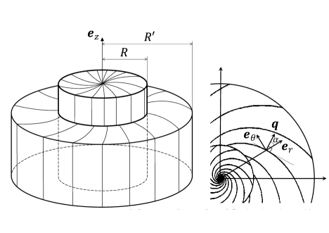
Figure 1: Left: The inner-cylinder of radius $R$ rotates as a solid-body within an outer cylinder at rest. The radius $R^{\prime}$ of the outer cylinder is taken as infinite. Right: The curved lines are perpendicular to q and describe logarithmic spirals. They correspond to the directions along which $\sigma=\sigma^{\perp}$ and $\mu=\mu^{\perp}$.

3 Induction equation

In the magnetohydrodynamic approximation, the Maxwell equations and Ohm’s law take the form

$${\bf H}=[\mu_{ij}]^{-1}{\bf B},$$ (6)

$${\bf J}=\nabla\times{\bf H},$$ (7)

$$\partial_{t}{\bf B}=-\nabla\times{\bf E}$$ (8)

$$\nabla\cdot{\bf B}=0,$$ (9)

$${\bf J}=[\sigma_{ij}]({\bf E}+{\bf U}\times{\bf B}),$$ (10)

where ${\bf H}$, ${\bf B}$, ${\bf J}$, ${\bf E}$ and ${\bf U}$ are the magnetic field, the induction field, the current density, the electric field and the velocity field. The induction equation then takes the form

$$\partial_{t}{\bf B}=\nabla\times({\bf U}\times{\bf B})-\nabla\times\left([\sigma_{ij}]^{-1}\nabla\times\left([\mu_{ij}]^{-1}{\bf B}\right)\right).$$ (11)

Renormalizing the distance, electrical conductivity, magnetic permeability and time by respectively $R,\mu^{\perp},\sigma^{\perp}$ and $\mu^{\perp}\sigma^{\perp}R^{2}$, the dimensionless form of the induction equation is identical to (11), but with

$$[\sigma_{ij}]^{-1} = \delta_{ij}+\sigma q_{i}q_{j},\;\;\;\sigma=\frac{\sigma^{\perp}}{\sigma^{\parallel}}-1,$$ (12)

$$[\mu_{ij}]^{-1} = \delta_{ij}+\mu q_{i}q_{j},\;\;\;\mu=\frac{\mu^{\perp}}{\mu^{\parallel}}-1$$ (13)

and

$${\bf U}=\left\{\begin{split}r\Omega{\bf e}_{\theta}&,&r<1\\ 0&,&r>1\end{split}\;\;\;,\right.$$ (14)

where $\Omega$ is the dimensionless angular velocity of the inner cylinder. We note that $(\sigma,\mu)\in[-1,+\infty[^{2}$, with $\sigma=0$ and $\mu=0$ corresponding to respectively isotropic conductivity and isotropic permeability.

Provided the velocity is stationary and $z$-independent, an axisymmetric magnetic induction can be searched in the form

$${\bf B}(r,z,t)=\tilde{B}{\bf e}_{\theta}+\nabla\times\left(\tilde{A}{\bf e}_{\theta}\right),$$ (15)

with $(\tilde{A},\tilde{B})=(A(r),B(r))\exp(\gamma t+\mathrm{i}kz)$, where $\gamma$ is the instability growth rate and $k$ the vertical wavenumber of the corresponding eigenmode, and where $A$ and $B$ depend only on the radial coordinate $r$. Thus the magnetic induction takes the form

$${\bf B}=\left(-\mathrm{i}kA,B,\frac{1}{r}\partial_{r}(rA)\right)\exp(\gamma t+\mathrm{i}kz),$$ (16)

with dynamo action corresponding to $\Re\{\gamma\}>0$.

From (14) and (16), it can be shown that $\nabla\times({\bf U}\times{\bf B})=0$ in each region $r<1$ and $r>1$ (see appendix A). Replacing (12), (13) and (16) into the induction equation (11) leads to

$$\gamma A+(1+\sigma s^{2})D_{k}(A)+\mu c^{2}k^{2}A = \mathrm{i}csk(\sigma-\mu)B,$$ (17)

$$\gamma B+(1+\mu s^{2})D_{k}(B)+\sigma c^{2}k^{2}B = -\mathrm{i}csk(\sigma-\mu)D_{k}(A),$$ (18)

where $D_{\nu}(X)=\nu^{2}X-\partial_{r}\left(\frac{1}{r}\partial_{r}(rX)\right)$. The derivation of (17) and (18) is given in appendix B. For $\sigma=\mu=0$, corresponding to isotropy of both conductivity and permeability, (17) and (18) are diffusion equations, leading to a free decaying solution (no dynamo action). For an isotropic permeability, $\mu=0$, (17) and (18) are identical to the equations derived in Plunian & Alboussière (2020).

4 Dynamo threshold

4.1 General form of the solutions

Looking for non-oscillating solutions, the dynamo threshold then corresponds to $\gamma=0$. Thus, taking $\gamma=0$ in (17) and (18), it can be shown (Appendix C) that

$$\left(D_{k_{\mu}}\circ D_{k_{\sigma}}\right)(A)=\left(D_{k_{\sigma}}\circ D_{k_{\mu}}\right)(B)=0,$$ (19)

where

$$k_{\sigma}=k\left(\frac{1+\sigma}{1+\sigma s^{2}}\right)^{1/2},\;\;\;\;\;k_{\mu}=k\left(\frac{1+\mu}{1+\mu s^{2}}\right)^{1/2}.$$ (20)

We note that the two operators $D_{k_{\sigma}}$ and $D_{k_{\mu}}$ are commutative. Therefore in (19) we can apply the two operators in the order we want, $D_{k_{\mu}}\circ D_{k_{\sigma}}$ or $D_{k_{\sigma}}\circ D_{k_{\mu}}$, to both $A$ and $B$. The set of functions $X(r)$, satisfying the fourth-order differential equation $\left(D_{k_{\mu}}\circ D_{k_{\sigma}}\right)(X)=0$, is a vector space of dimension 4. Now, we know that, whatever $\nu$, the solutions of $D_{\nu}(X)=0$ are a linear combination of $I_{1}(\nu r)$ and $K_{1}(\nu r)$, where $I_{1}$ and $K_{1}$ are modified Bessel functions of first and second kind, of order 1. Therefore the solutions of (19) are a linear combination of $I_{1}(k_{\sigma}r)$, $K_{1}(k_{\sigma}r)$, $I_{1}(k_{\mu}r)$ and $K_{1}(k_{\mu}r)$.

Looking for $A$ in the form

$$A=\alpha_{\sigma}I_{1}(k_{\sigma}r)+\beta_{\sigma}K_{1}(k_{\sigma}r)+\alpha_{\mu}I_{1}(k_{\mu}r)+\beta_{\mu}K_{1}(k_{\mu}r),$$ (21)

and specifying that $A$ must be finite at $r=0$ and that $\lim\limits_{r\to\infty}A=0$, leads to

$$A= \left\{\begin{split}r<1,&\;\;\;\;\;\alpha_{\sigma}I_{1}(k_{\sigma}r)+\alpha_{\mu}I_{1}(k_{\mu}r)&\\ r>1,&\;\;\;\;\;\beta_{\sigma}K_{1}(k_{\sigma}r)+\beta_{\mu}K_{1}(k_{\mu}r)&\end{split}\right.,$$ (22)

where $\alpha_{\sigma}$, $\beta_{\sigma}$, $\alpha_{\mu}$ and $\beta_{\mu}$ are free parameters that will be constrained by additional boundary conditions at $r=1$. Replacing (22) in (17) for $\gamma=0$ leads to the following expression for $B$

$$B= \left\{\begin{split}r<1,&\;\;\;\frac{\mathrm{i}ck}{s}\left(\alpha_{\sigma}I_{1}(k_{\sigma}r)+\frac{\mu s^{2}}{1+\mu s^{2}}\alpha_{\mu}I_{1}(k_{\mu}r)\right)&\\ r>1,&\;\;\;\frac{\mathrm{i}ck}{s}\left(\beta_{\sigma}K_{1}(k_{\sigma}r)+\frac{\mu s^{2}}{1+\mu s^{2}}\beta_{\mu}K_{1}(k_{\mu}r)\right)&\end{split}\right.,$$ (23)

the derivation of which being given in Appendix D.

4.2 Boundary conditions at $r=1$

From the Maxwell equations and Green-Ostrogradski and Stokes theorems, the radial component of ${\bf B}$ and the tangential components of ${\bf H}=[\mu_{ij}]^{-1}{\bf B}$ must be continuous at $r=1$. Taking the expression of ${\bf B}$ and ${\bf H}$ given in (16) and (49), these continuity conditions can be written in terms of $A$ and $B$ as

$$A(r=1^{-}) = A(r=1^{+}),$$ (24)

$$B(r=1^{-}) = B(r=1^{+}),$$ (25)

$$\partial_{r}A(r=1^{-}) = \partial_{r}A(r=1^{+}).$$ (26)

Taking $A$ and $B$ given in (22) and (23) and replacing them in (24), (25) and (26) leads to (Appendix E)

$$\alpha_{\sigma}I_{1}(k_{\sigma})-\beta_{\sigma}K_{1}(k_{\sigma}) = 0$$ (27)

$$\alpha_{\mu}I_{1}(k_{\mu})-\beta_{\mu}K_{1}(k_{\mu}) = 0$$ (28)

$$\alpha_{\sigma}k_{\sigma}I_{0}(k_{\sigma})+\alpha_{\mu}k_{\mu}I_{0}(k_{\mu})+\beta_{\sigma}k_{\sigma}K_{0}(k_{\sigma})+\beta_{\mu}k_{\mu}K_{0}(k_{\mu}) = 0,$$ (29)

where $I_{0}$ and $K_{0}$ are modified Bessel functions of first and second kind, of order 0. It is convenient to introduce the parameters $\lambda_{\sigma}=\alpha_{\sigma}I_{1}(k_{\sigma})\mathrm{i}k/s$ and $\lambda_{\mu}=\alpha_{\mu}I_{1}(k_{\mu})\mathrm{i}k/s$. Then, using (27) and (28), we can rewrite $A$ and $B$ in the following form:

$$\mathrm{i}kA= \left\{\begin{split}r<1,&\;\;\;\;\;s\left(\lambda_{\sigma}\frac{I_{1}(k_{\sigma}r)}{I_{1}(k_{\sigma})}+\lambda_{\mu}\frac{I_{1}(k_{\mu}r)}{I_{1}(k_{\mu})}\right)&\\ r>1,&\;\;\;\;\;s\left(\lambda_{\sigma}\frac{K_{1}(k_{\sigma}r)}{K_{1}(k_{\sigma})}+\lambda_{\mu}\frac{K_{1}(k_{\mu}r)}{K_{1}(k_{\mu})}\right)&\end{split}\right.,$$ (30)

$$B= \left\{\begin{split}r<1,&\;\;\;c\left(\lambda_{\sigma}\frac{I_{1}(k_{\sigma}r)}{I_{1}(k_{\sigma})}+\frac{\mu s^{2}}{1+\mu s^{2}}\lambda_{\mu}\frac{I_{1}(k_{\mu}r)}{I_{1}(k_{\mu})}\right)&\\ r>1,&\;\;\;c\left(\lambda_{\sigma}\frac{K_{1}(k_{\sigma}r)}{K_{1}(k_{\sigma})}+\frac{\mu s^{2}}{1+\mu s^{2}}\lambda_{\mu}\frac{K_{1}(k_{\mu}r)}{K_{1}(k_{\mu})}\right)&\end{split}\right..$$ (31)

The continuity of $\partial_{r}A$ at $r=1$, given by (29), then leads to the following identity between $\lambda_{\sigma}$ and $\lambda_{\mu}$

$$\lambda_{\sigma}\Gamma(k_{\sigma})+\lambda_{\mu}\Gamma(k_{\mu})=0,$$ (32)

with

$$\Gamma(x)=x\left(\frac{I_{0}(x)}{I_{1}(x)}+\frac{K_{0}(x)}{K_{1}(x)}\right)\equiv\left(I_{1}(x)K_{1}(x)\right)^{-1},$$ (33)

the last equality coming from the Wronskian relation

$$I_{m}(x)K_{m+1}(x)+I_{m+1}(x)K_{m}(x)=1/x.$$ (34)

In figure 2 the eigenmodes $\mathrm{i}kA$ and $B$ are plotted versus $r$ for $\lambda_{\sigma}=\Gamma(k_{\mu})$ and $\lambda_{\mu}=-\Gamma(k_{\sigma})$ such that (32) is satisfied.

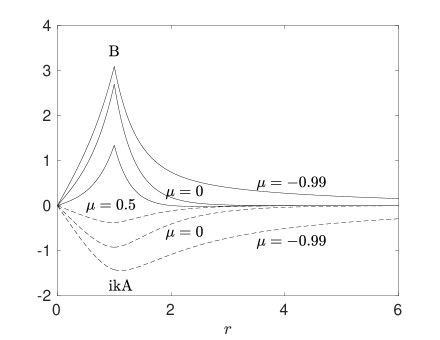
Figure 2: Eigenmodes $\mathrm{i}kA$ (dashed lines) and $B$ (solid lines) versus $r$, for $\sigma=10^{6},k=1.1,\alpha=0.16\pi$, $\lambda_{\sigma}=\Gamma(k_{\mu})$, $\lambda_{\mu}=-\Gamma(k_{\sigma})$ and for $\mu\in\{-0.99,0,0.5\}$.

Finally, the tangential components ${\bf E}_{\theta}$ and ${\bf E}_{z}$ of the electric field

$${\bf E}=-{\bf U}\times{\bf B}+[\sigma_{ij}]^{-1}{\bf J}$$ (35)

have to be continuous at $r=1$. The expression of the current density ${\bf J}$, which is derived in Appendix F, is given by

$${\bf J}_{r}= -\mathrm{i}ck\lambda_{\sigma}\left\{\begin{split}r<1,&\;\;\;I_{1}(k_{\sigma}r)/I_{1}(k_{\sigma})\\ r>1,&\;\;\;K_{1}(k_{\sigma}r)/K_{1}(k_{\sigma})\end{split}\right.,$$ (36)

$${\bf J}_{\theta}= -\frac{\sigma sc}{1+\sigma s^{2}}{\bf J}_{r},$$ (37)

$${\bf J}_{z}= ck_{\sigma}\lambda_{\sigma}\left\{\begin{split}r<1,&\;\;\;I_{0}(k_{\sigma}r)/I_{1}(k_{\sigma})\\ r>1,&\;\;\;-K_{0}(k_{\sigma}r)/K_{1}(k_{\sigma})\end{split}\right.,$$ (38)

where the coefficient $\exp(\mathrm{i}kz)$ has been dropped for convenience.

From (12), (14) and (37), we find that ${\bf E}_{\theta}=0$, which is in agreement with axisymmetric solutions. Indeed, Maxwell equation (8) taken at the threshold implies $\nabla\times{\bf E}=0$. Applying the Stokes theorem to the integral of $\nabla\times{\bf E}$ on a disc of radius $r$, and assuming axisymmetry, then leads to ${\bf E}_{\theta}(r)=0$.

The continuity of ${\bf E}_{z}$ implies the following identity:

$$({\bf J}_{z}+r\Omega{\bf B}_{r})(r=1^{-})={\bf J}_{z}(r=1^{+}).$$ (39)

Replacing (30) and (38) in (39), and using (32), leads to the dynamo threshold

$$\Omega^{c}=\frac{c}{s}\left(I_{1}(k_{\sigma})K_{1}(k_{\sigma})-I_{1}(k_{\mu})K_{1}(k_{\mu})\right)^{-1}.$$ (40)

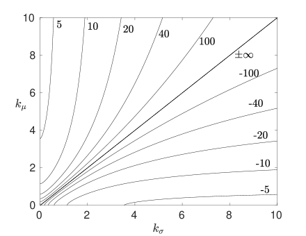
Figure 3: Isovalues of $\Omega^{c}\in\{\pm 5,\pm 10,\pm 20,\pm 40,\pm 100\}$ in the ($k_{\sigma},k_{\mu}$) map, for $\alpha=0.16\pi$. The diagonal $k_{\sigma}=k_{\mu}$ corresponds to $\Omega^{c}\rightarrow\pm\infty$.

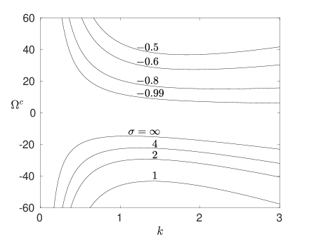
Figure 4: Curves of the dynamo threshold $\Omega^{c}$ versus $k$, for $\mu=0$, $\alpha=0.16\pi$ and $\sigma\in\{-0.99,-0.8,-0.6,-0.5,1,2,4,+\infty\}$.

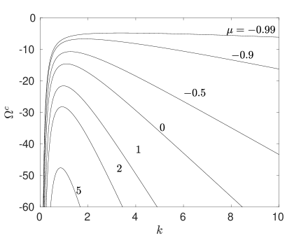
Figure 5: Curves of the dynamo threshold $\Omega^{c}$ versus $k$, for $\sigma=10^{5}$, $\alpha=0.16\pi$ and $\mu\in\{-0.99,-0.9,-0.5,0,1,2,5\}$.

5 Analysis of the results

5.1 Dispersion relation

A striking consequence of (40) is that $\Omega^{c}(\sigma,\mu)$ is antisymmetric, satisfying

$$\Omega^{c}(\sigma,\mu)=-\Omega^{c}(\mu,\sigma).$$ (41)

In addition for identical anisotropies of conductivity and permeability, $\mu=\sigma$, the threshold is infinite, leading to the impossibility of an axisymmetric dynamo,

$$\lim\limits_{|\sigma-\mu|\rightarrow 0}|\Omega^{c}(\sigma,\mu)|\rightarrow+\infty.$$ (42)

This is illustrated in figure 3, in which the curves of a few isovalues of $\Omega^{c}$ are plotted versus $k_{\sigma}$ and $k_{\mu}$. In particular, having both $\sigma\gg 1$ and $\mu\gg 1$ is detrimental for dynamo action, as in this case, from (20), $k_{\sigma}\approx k_{\mu}\approx k/s$.

The antisymmetry property (41) of $\Omega^{c}(\sigma,\mu)$ can also be derived directly from the set of equations (17-18) taken for $\gamma=0$, the boundary conditions (24-26) and (39), without deriving explicitly the expressions of $A$ and $B$. This is shown in Appendix G.

Alternatively, changing $\alpha$ to $-\alpha$ in (40) also changes $\Omega^{c}$ to $-\Omega^{c}$. This can be also derived directly from (17-18), taken for $\gamma=0$, the boundary conditions (24-26), and (39), by changing $A$ to $-A$ (or $B$ to $-B$).

We check that for an isotropic permeability, $\mu=0$, $\Omega^{c}$ is the same as that given in Plunian & Alboussière (2020). In figure 4 the curves of the dynamo threshold $\Omega^{c}$ versus $k$ are plotted for $\mu=0$ (isotropic magnetic permeability), $\alpha=0.16\pi$ and different values of $\sigma$. The negative values of $\sigma$ correspond to an electrical conductivity that is the highest in the direction parallel to q.

In figure 5 the curves of the dynamo threshold $\Omega^{c}$ versus $k$ are plotted for $\sigma=10^{5}$, $\alpha=0.16\pi$ and different values of $\mu$. For $\mu=0$, the minimum value of $|\Omega^{c}|$ is obtained for $k=1.1$ and $\alpha=0.16\pi$, and is equal to $\min_{k,\alpha}|\Omega^{c}|=14.61$ (Plunian & Alboussière, 2020). For positive values of $\mu$, $|\Omega^{c}|$ increases with $\mu$, showing the detrimental effect of having both a high $\sigma$ and a high $\mu$. For negative values of $\mu$, $|\Omega^{c}|$ decreases with $|\mu|$, showing that the dynamo effect is favoured if the permeability is higher in the direction parallel to q.

For $s=0$ (radial q) or $c=0$ (azimuthal q), the dynamo is impossible. This is obvious for $s=0$ as the threshold given by (40) is infinite. For $c=0$, (31) implies that $B=0$. In addition, as $s^{2}=1$, (20) implies that $k_{\sigma}=k_{\mu}=k$. Then, from (30) and (32), we find that $A=0$.

5.2 Current density

Concerning the current density ${\bf J}$, given at the threshold by (36-38), we note that it only depends on $\sigma$, and not on $\mu$. In other words, taking an anisotropic magnetic permeability $\mu\neq 0$ does not change the geometry of the current density with respect to the isotropic case $\mu=0$.

For an isotropic conductivity $\sigma=0$, we find that ${\bf J}_{\theta}=0$. This corresponds to the neutral point argument of Cowling (1934), after which a toroidal current density cannot be produced if axisymmetry is assumed. However, and although such a neutral point argument is satisfied for $\sigma=0$, this does not exclude the possibility of dynamo action for an anisotropic magnetic permeability $\mu\neq 0$.

From (37), we note that the projection in the ($r$,$\theta$) plane of the current density ${\bf J}$ describes spiralling trajectories. In the limit $\sigma\rightarrow+\infty$, we find that ${\bf J}\cdot\textit{{q}}=0$.

5.3 Magnetic induction

From the expression of ${\bf B}$ given in (16), and applying (30), (31) and (77), leads to the following expressions for the magnetic induction components

$${\bf B}_{r}= -s\left\{\begin{split}r<1,&\;\;\;\lambda_{\sigma}\frac{I_{1}(k_{\sigma}r)}{I_{1}(k_{\sigma})}+\lambda_{\mu}\frac{I_{1}(k_{\mu}r)}{I_{1}(k_{\mu})}\\ r>1,&\;\;\;\lambda_{\sigma}\frac{K_{1}(k_{\sigma}r)}{K_{1}(k_{\sigma})}+\lambda_{\mu}\frac{K_{1}(k_{\mu}r)}{K_{1}(k_{\mu})}\end{split}\right.,$$ (43)

$${\bf B}_{\theta}= c\left\{\begin{split}r<1,&\;\;\;\lambda_{\sigma}\frac{I_{1}(k_{\sigma}r)}{I_{1}(k_{\sigma})}+\lambda_{\mu}\left(\frac{\mu s^{2}}{1+\mu s^{2}}\right)\frac{I_{1}(k_{\mu}r)}{I_{1}(k_{\mu})}\\ r>1,&\;\;\;\lambda_{\sigma}\frac{K_{1}(k_{\sigma}r)}{K_{1}(k_{\sigma})}+\lambda_{\mu}\left(\frac{\mu s^{2}}{1+\mu s^{2}}\right)\frac{K_{1}(k_{\mu}r)}{K_{1}(k_{\mu})}\end{split}\right.,$$ (44)

$${\bf B}_{z}= -\frac{\mathrm{i}s}{k}\left\{\begin{split}r<1,&\;\;\;\lambda_{\sigma}k_{\sigma}\frac{I_{0}(k_{\sigma}r)}{I_{1}(k_{\sigma})}+\lambda_{\mu}k_{\mu}\frac{I_{0}(k_{\mu}r)}{I_{1}(k_{\mu})}\\ r>1,&\;\;\;-\lambda_{\sigma}k_{\sigma}\frac{K_{0}(k_{\sigma}r)}{K_{1}(k_{\sigma})}-\lambda_{\mu}k_{\mu}\frac{K_{0}(k_{\mu}r)}{K_{1}(k_{\mu})}\end{split}\right.,$$ (45)

where, again, the coefficient $\exp(\mathrm{i}kz)$ has been dropped for convenience. In contrast to ${\bf J}$, the induction field depends not only on $\sigma$, but also on $\mu$, implying the following remarks.

In the case of identical anisotropic conductivity and permeability, $\sigma=\mu$, as mentioned earlier the dynamo is impossible. From (20) and (32) we have $k_{\sigma}=k_{\mu}$ and $\lambda_{\sigma}+\lambda_{\mu}=0$, implying that ${\bf B}_{r}={\bf B}_{z}=0$. In that case the induction field ${\bf B}$ is then purely toroidal. This is in agreement with the antidynamo theorem of Kaiser et al. (1994), after which an invisible dynamo, with a purely toroidal magnetic field, is impossible.

In the limit $\mu\rightarrow\infty$, from (43) and (44) we have $c{\bf B}_{r}=-s{\bf B}_{\theta}$, implying that ${\bf B}\cdot\textit{{q}}=0$. The projection in the ($r$,$\theta$) plane of the induction field ${\bf B}$ thus describes spiralling trajectories perpendicular to q.

In figure 6 the current lines of ${\bf B}$ and ${\bf J}$ are plotted in the horizontal plane for different values of $(\sigma,\mu)$. In figures 6a, 6b and 6c, $\sigma=10^{5}$ and $\mu\in\{-0.99;0;5\}$. The current lines of ${\bf J}$ are identical because, as previously seen, ${\bf J}$ does not depend on $\mu$. From 6a to 6c, increasing $\mu$ has the effect of distorting the ${\bf B}$ current lines in the outer cylinder, such that the current lines of ${\bf B}$ reach the same curvature as the current lines of ${\bf J}$, which eventually is detrimental to dynamo action. In figures 6d, 6e and 6f, $\mu=10^{5}$ and $\sigma\in\{-0.99;0;10\}$. From 6d to 6f, increasing $\sigma$ has the effect of distorting the ${\bf J}$ current lines in both inner and outer cylinders, such that the current lines of ${\bf J}$ reach the same curvature direction as the current lines of ${\bf B}$, which ultimately is again detrimental to the dynamo action. We note that the ${\bf J}$ current lines in figures 6a, 6b and 6c and the ${\bf B}$ current lines in figures 6d, 6e and 6f are identical. This is because $\sigma\gg 1$ in figures 6a, 6b and 6c, implying ${\bf J}\cdot\textit{{q}}\approx 0$, and $\mu\gg 1$ in figures 6d, 6e and 6f, implying ${\bf B}\cdot\textit{{q}}\approx 0$.

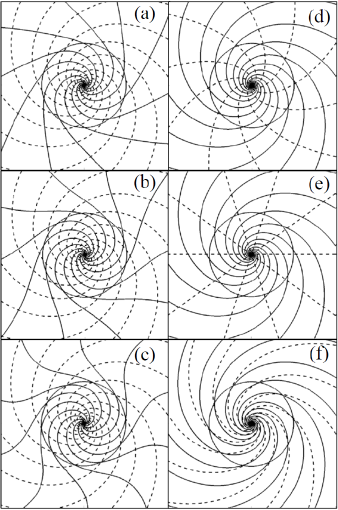
Figure 6: Current lines of ${\bf B}$ (solid lines) and ${\bf J}$ (dashed lines) in the horizontal plane for $\alpha=0.16\pi$, $k=1.1$, and for (a) $(\sigma,\mu)=(10^{5},-0.99)$, (b) $(\sigma,\mu)=(10^{5},0)$, (c) $(\sigma,\mu)=(10^{5},5)$, (d) $(\sigma,\mu)=(-0.99,10^{5})$, (e) $(\sigma,\mu)=(0,10^{5})$, (f) $(\sigma,\mu)=(10,10^{5})$.

6 Dynamo mechanism

The set of equations (17-18) can be rewritten in terms of ${\bf B}_{r}$ and ${\bf B}_{\theta}$ as

$$\gamma{\bf B}_{r} = cs(\sigma-\mu)k^{2}{\bf B}_{\theta}-(1+\sigma s^{2})D_{\tilde{k}_{\sigma\mu}}({\bf B}_{r})$$ (46)

$$\gamma{\bf B}_{\theta} = cs(\sigma-\mu)D_{k}({\bf B}_{r})-(1+\mu s^{2})D_{\tilde{k}_{\mu\sigma}}({\bf B}_{\theta}),$$ (47)

with

$$\tilde{k}_{\sigma\mu}=k\left(1+\frac{\mu c^{2}}{1+\sigma s^{2}}\right)^{1/2},\;\;\;\;\;\tilde{k}_{\mu\sigma}=k\left(1+\frac{\sigma c^{2}}{1+\mu s^{2}}\right)^{1/2}.$$ (48)

On the right hand side of each equation (46) and (47), the first term is a source term for the dynamo effect, while the second term is a decay term. In (46), resp. (47), the term $cs(\sigma-\mu)k^{2}{\bf B}_{\theta}$, resp. $cs(\sigma-\mu)D_{k}({\bf B}_{r})$, corresponds to the generation of ${\bf B}_{r}$ from ${\bf B}_{\theta}$, resp. ${\bf B}_{\theta}$ from ${\bf B}_{r}$. The differential rotation between the inner and outer cylinders also participates in the generation of ${\bf B}_{\theta}$ from ${\bf B}_{r}$, through the boundary condition (39). The latter is, however, not sufficient in itself. Therefore, it is clear why increasing the value of $|\sigma-\mu|$ helps for the dynamo effect, and why the dynamo is impossible for $\sigma=\mu$. Dynamo action thus occurs through differential rotation conjugated to anisotropic diffusion.

From the point of view of basic Maxwell and Ohm equations, and in the case of an isotropic conductivity ($\sigma=0$) and anisotropic magnetic permeability ($\mu\neq 0$), dynamo action can be understood in the following way. Suppose there exists an axisymmetric magnetic induction disturbance with a non-zero radial component ${\bf B}_{r}$ at some height $z$ along the shear zone ($r=1$). Ohm’s law (10) then drives two opposite currents in the axial direction ${\bf e}_{z}$ within the rotor and stator. In a medium of isotropic electrical conductivity, this current forms closed loops in the meridian planes, as can be seen in Fig. 6(e). From Ampère’s law (7), this generates an azimuthal magnetic field ${\bf H}_{\theta}$. Finally from (6), a radial component of the induction vector ${\bf B}_{r}$ is generated from ${{\bf H}_{\theta}}$ because of the anisotropic magnetic permeability. Depending on the orientation of the anisotropic permeability tensor and the direction of the solid rotation, the generated ${\bf B}_{r}$ can either reinforce (dynamo action is possible) or oppose the initial seed of radial magnetic induction (no dynamo).

7 Conclusions

For an anisotropic electrical conductivity ($\sigma^{\perp}\neq\sigma^{\parallel}$) conjugated to an anisotropic magnetic permeability ($\mu^{\perp}\neq\mu^{\parallel}$), we could think that maximizing the ratio $(\sigma^{\perp}\mu^{\perp})/(\sigma^{\parallel}\mu^{\parallel})$ could help for the dynamo action. This would correspond to minimizing magnetic diffusivity in the perpendicular direction relative to that in the parallel direction. This is not true for two reasons. First, contrary to the isotropic case, defining an anisotropic magnetic diffusivity is meaningless, because the electrical conductivity and magnetic permeability are now tensors. Second, it has been shown that taking $\sigma^{\perp}/\sigma^{\parallel}\gg 1$ and $\mu^{\perp}/\mu^{\parallel}\gg 1$ is in fact highly detrimental to the dynamo effect, these two conditions having the effect of aligning the current lines of respectively the current density ${\bf J}$ and magnetic induction ${\bf B}$ in the same direction $\textit{{q}}^{\perp}$. In contrast, having $\sigma^{\perp}/\sigma^{\parallel}\gg 1$ and $\mu^{\perp}/\mu^{\parallel}=1$, or $\sigma^{\perp}/\sigma^{\parallel}=1$ and $\mu^{\perp}/\mu^{\parallel}\gg 1$ leads to the same dynamo threshold $|\Omega^{c}|=14.61$, for $k=1.1$ and $\alpha=0.16\pi$.

As an application let us consider an experimental demonstration of the dynamo effect based on such conductivity and permeability spiral anisotropy, with differential rotation between two cylinders, as sketched in figure 1. An anisotropic conductivity, resp. permeability, can be manufactured by alternating thin layers of two materials with different conductivities, resp. permeabilities. Although the resulting medium is no longer axisymmetric, our model is still a good approximation of such an experiment. To realize the first case $\sigma^{\perp}/\sigma^{\parallel}\gg 1$ and $\mu^{\perp}/\mu^{\parallel}=1$, we can alternate spiral layers of a high electrical conductivity material, e.g. copper, and a material which is electrically insulating, e.g. epoxy resin, both having a relative magnetic permeability equal to unity. To realize the second case $\sigma^{\perp}/\sigma^{\parallel}=1$ and $\mu^{\perp}/\mu^{\parallel}\gg 1$ , we can alternate spiral layers of a high magnetic permeability material, e.g. $\mu$-metal (permalloy), and a material with a relative magnetic permeability equal to unity, e.g. stainless steel, both having approximately the same electrical conductivity. The current lines of ${\bf B}$ and ${\bf J}$ of these two cases are illustrated in figure 6b and 6e. For the second case, a crucial issue will be to guarantee a good electrical contact between both materials, $\mu$-metal and stainless steel. Indeed, if this is not the case, this would correspond to having $\sigma^{\perp}/\sigma^{\parallel}\gg 1$ and $\mu^{\perp}/\mu^{\parallel}\gg 1$ which, again, would be highly detrimental to the dynamo effect.

In the case of an isotropic electrical conductivity, $\sigma^{\perp}/\sigma^{\parallel}=1$, and as illustrated in figure 6e, the azimuthal current density is null, ${\bf J}_{\theta}=0$ , which is in agreement with the neutral point argument of Cowling. As ${\bf J}=\nabla\times{\bf H}$, this implies that the circulation of the poloidal component of ${\bf H}$ on a closed current line is zero (Cowling, 1934). However, as shown in (49), in the case of an anisotropic magnetic permeability this does not imply that the poloidal component of ${\bf B}$ is zero. Therefore, although the neutral point argument of Cowling still holds, it does not imply the impossibility of a dynamo effect.

Appendix A Derivation of $\nabla\times({\bf U}\times{\bf B})=0$

Assuming axisymmetry ($\partial_{\theta}=0$), the curl of the cross product of ${\bf U}=r\Omega{\bf e}_{\theta}$ and ${\bf B}=\left(B_{r},B_{\theta},B_{z}\right)$ is given by $\nabla\times({\bf U}\times{\bf B})=\left(\partial_{z}(r\Omega B_{z})+\partial_{r}(r\Omega B_{r})\right){\bf e}_{\theta}$. Assuming that $\Omega$ is constant in space and using the solenoidality of ${\bf B}$, $\nabla\cdot{\bf B}=0$, leads to $\nabla\times({\bf U}\times{\bf B})=0$.

Appendix B Derivation of (17) and (18)

The product of $[\mu_{ij}]^{-1}=\begin{pmatrix}1+\mu c^{2}&\mu cs&0\\ \mu cs&1+\mu s^{2}&0\\ 0&0&1\end{pmatrix}$ given by (13), and the induction field ${\bf B}=\begin{pmatrix}-\mathrm{i}kA\\ B\\ \frac{1}{r}\partial_{r}(rA)\end{pmatrix}\exp(\gamma t+\mathrm{i}kz)$ given by (16), leads to the magnetic field

$${\bf H}=[\mu_{ij}]^{-1}{\bf B}=\begin{pmatrix}-\mathrm{i}k(1+\mu c^{2})A+\mu csB\\ -\mathrm{i}k\mu csA+(1+\mu s^{2})B\\ \frac{1}{r}\partial_{r}(rA)\end{pmatrix},$$ (49)

where, from now, the exponential term is dropped for convenience. Assuming axisymmetry, the curl of ${\bf H}$ takes the form $\nabla\times{\bf H}=\begin{pmatrix}-\mathrm{i}kH_{\theta}\\ \mathrm{i}kH_{r}-\partial_{r}H_{z}\\ \frac{1}{r}\partial_{r}(rH_{\theta})\end{pmatrix}$, leading to the current density

$${\bf J}=\nabla\times{\bf H}=\begin{pmatrix}-k^{2}\mu csA-\mathrm{i}k(1+\mu s^{2})B\\ D_{k}(A)+\mu c^{2}k^{2}A+\mathrm{i}\mu cskB\\ -\mathrm{i}\mu csk\frac{1}{r}\partial_{r}(rA)+(1+\mu s^{2})\frac{1}{r}\partial_{r}(rB)\end{pmatrix},$$ (50)

where $D_{\nu}(X)=\nu^{2}X-\partial_{r}\left(\frac{1}{r}\partial_{r}(rX)\right)$. The product of $[\sigma_{ij}]^{-1}=\begin{pmatrix}1+\sigma c^{2}&\sigma cs&0\\ \sigma cs&1+\sigma s^{2}&0\\ 0&0&1\end{pmatrix}$ given by (12), and ${\bf J}$ given by (50), leads to

$$[\sigma_{ij}]^{-1}{\bf J}=\begin{pmatrix}-k^{2}\mu csA+\sigma csD_{k}(A)-\mathrm{i}k(1+\sigma c^{2}+\mu s^{2})B\\ \mu c^{2}k^{2}A+(1+\sigma s^{2})D_{k}(A)-\mathrm{i}csk(\sigma-\mu)B\\ -\mathrm{i}\mu csk\frac{1}{r}\partial_{r}(rA)+(1+\mu s^{2})\frac{1}{r}\partial_{r}(rB)\end{pmatrix}.$$ (51)

Taking the curl leads to $\nabla\times[\sigma_{ij}]^{-1}{\bf J}=\begin{pmatrix}-\mathrm{i}kF\\ G\\ \frac{1}{r}\partial_{r}(rF)\end{pmatrix},$ with

$$F = \mu c^{2}k^{2}A+(1+\sigma s^{2})D_{k}(A)-\mathrm{i}kcs(\sigma-\mu)B,$$ (52)

$$G = \mathrm{i}kcs(\sigma-\mu)D_{k}(A)+\sigma k^{2}c^{2}B+(1+\mu s^{2})D_{k}(B).\;\;\;\;\;\;\;$$ (53)

As $\nabla\times({\bf U}\times{\bf B})=0$, the induction equation (11) is reduced to $\partial_{t}{\bf B}=-\nabla\times[\sigma_{ij}]^{-1}{\bf J}$, leading to

$$\gamma A = -F,$$ (54)

$$\gamma B = -G,$$ (55)

$$\frac{\gamma}{r}\partial_{r}(rA) = -\frac{1}{r}\partial_{r}(rF),$$ (56)

and then to (17) and (18).

Appendix C Derivation of the fourth-order differential equation (19) satisfied by $A$ and $B$ at the dynamo threshold

Replacing $\gamma=0$ in (17) and (18) leads to the following system

$$(1+\sigma s^{2})D_{k}(A)+\mu c^{2}k^{2}A = \mathrm{i}csk(\sigma-\mu)B,$$ (57)

$$(1+\mu s^{2})D_{k}(B)+\sigma c^{2}k^{2}B = -\mathrm{i}csk(\sigma-\mu)D_{k}(A),\;\;\;\;\;$$ (58)

where, again, $D_{\nu}(X)=\nu^{2}X-\partial_{r}\left(\frac{1}{r}\partial_{r}(rX)\right)$.

It is straightforward to show that

$$(1+\sigma s^{2})D_{k}(X)=(1+\sigma s^{2})D_{k_{\sigma}}(X)-\sigma c^{2}k^{2}X,\;\;\;\;\;$$ (59)

$$(1+\mu s^{2})D_{k}(X)=(1+\mu s^{2})D_{k_{\mu}}(X)-\mu c^{2}k^{2}X,\;\;\;\;\;$$ (60)

where $k_{\sigma}$ and $k_{\mu}$ are defined in (20) and that we rewrite here for convenience

$$k_{\sigma}=k\left(\frac{1+\sigma}{1+\sigma s^{2}}\right)^{1/2},\;\;\;\;\;k_{\mu}=k\left(\frac{1+\mu}{1+\mu s^{2}}\right)^{1/2}.$$

Using (59) and (60) in (57) and (58) then leads to

$$(1+\sigma s^{2})D_{k_{\sigma}}(A) = ck(\sigma-\mu)(ckA+\mathrm{i}sB),$$ (61)

$$(1+\mu s^{2})D_{k_{\mu}}(B) = -ck(\sigma-\mu)(ckB+\mathrm{i}sD_{k}(A)).\;\;\;\;\;$$ (62)

Then to obtain (19) we need to demonstrate that $D_{k_{\mu}}(ckA+\mathrm{i}sB)=0$ and $D_{k_{\sigma}}(ckB+\mathrm{i}sD_{k}(A))=0$. For that, we rewrite (57) and (58) as

$$D_{k}(A) = \sigma\left(-s^{2}D_{k}(A)+\mathrm{i}cskB\right)-\mu\left(c^{2}k^{2}A+\mathrm{i}cskB\right),$$ (63)

$$D_{k}(B) = -\sigma\left(c^{2}k^{2}B+\mathrm{i}cskD_{k}(A)\right)+\mu D_{k}\left(-s^{2}B+\mathrm{i}cskA\right).$$ (64)

Multiplying (63) by $ck$, (64) by $\mathrm{i}s$, and adding both quantities leads to

$$(1+\mu s^{2})D_{k}(ckA+\mathrm{i}sB)=-\mu c^{2}k^{2}(ckA+\mathrm{i}sB),$$ (65)

which, from (60) with $X=ckA+\mathrm{i}sB$, is equivalent to

$$D_{k_{\mu}}(ckA+\mathrm{i}sB)=0.$$ (66)

Applying (66) to (61) then leads to

$$\left(D_{k_{\mu}}\circ D_{k_{\sigma}}\right)(A)=0.$$ (67)

Taking $D_{k}$ of (63) multiplied by $\mathrm{i}s$ on the one hand, and (64) multiplied by $ck$ on the other hand, and adding both quantities leads to

$$(1+\sigma s^{2})D_{k}(ckB+\mathrm{i}sD_{k}(A))=-\sigma c^{2}k^{2}(ckB+\mathrm{i}sD_{k}(A)),$$ (68)

which, from (59) with $X=ckB+\mathrm{i}sD_{k}(A)$, is equivalent to

$$D_{k_{\sigma}}(ckB+\mathrm{i}sD_{k}(A))=0.$$ (69)

Applying (69) to (62) leads to

$$\left(D_{k_{\sigma}}\circ D_{k_{\mu}}\right)(B)=0,$$ (70)

which, together with (67), corresponds to (19).

Appendix D Derivation of $B$, given in (23), at the dynamo threshold

Starting from (22), which we rewrite here as

$$A= \left\{\begin{split}r<1,&\;\;\;\;\;\alpha_{\sigma}I_{1}(k_{\sigma}r)+\alpha_{\mu}I_{1}(k_{\mu}r)&\\ r>1,&\;\;\;\;\;\beta_{\sigma}K_{1}(k_{\sigma}r)+\beta_{\mu}K_{1}(k_{\mu}r)&\end{split}\right.,$$

we will derive $B$ from (17), which we write here for $\gamma=0$ as

$$B=\left((1+\sigma s^{2})D_{k}(A)+\mu c^{2}k^{2}A\right)/\left(\mathrm{i}csk(\sigma-\mu)\right).\\$$ (71)

Using the relations (59) and (60), and knowing that, whatever $\nu$, $D_{\nu}(I_{1}(k_{\nu}r))=D_{\nu}(K_{1}(k_{\nu}r))=0$ we find that

$$D_{k}(A)=\left\{\begin{split}r<1,&\;\;\;-\frac{\sigma c^{2}k^{2}}{1+\sigma s^{2}}\alpha_{\sigma}I_{1}(k_{\sigma}r)-\frac{\mu c^{2}k^{2}}{1+\mu s^{2}}\alpha_{\mu}I_{1}(k_{\mu}r)&\\ r>1,&\;\;\;-\frac{\sigma c^{2}k^{2}}{1+\sigma s^{2}}\beta_{\sigma}K_{1}(k_{\sigma}r)-\frac{\mu c^{2}k^{2}}{1+\mu s^{2}}\beta_{\mu}K_{1}(k_{\mu}r)&\end{split}\right..$$ (72)

Then, replacing in (71) the expressions of $A$ and $D_{k}(A)$ given by (22) and (72) leads to the following expression for $B$, which is also given in (23):

$$B= \left\{\begin{split}r<1,&\;\;\;\frac{\mathrm{i}ck}{s}\left(\alpha_{\sigma}I_{1}(k_{\sigma}r)+\frac{\mu s^{2}}{1+\mu s^{2}}\alpha_{\mu}I_{1}(k_{\mu}r)\right)&\\ r>1,&\;\;\;\frac{\mathrm{i}ck}{s}\left(\beta_{\sigma}K_{1}(k_{\sigma}r)+\frac{\mu s^{2}}{1+\mu s^{2}}\beta_{\mu}K_{1}(k_{\mu}r)\right)&\end{split}\right..$$

Appendix E Derivation of the boundary conditions (27), (28) and (29) at the dynamo threshold

The continuity of $A$ and $B$ at $r=1$, taken from their expressions (22) and (23), takes the following form:

$$\alpha_{\sigma}I_{1}(k_{\sigma})+\alpha_{\mu}I_{1}(k_{\mu}) = \beta_{\sigma}K_{1}(k_{\sigma})+\beta_{\mu}K_{1}(k_{\mu})$$ (73)

$$\alpha_{\sigma}I_{1}(k_{\sigma})+\frac{\mu s^{2}}{1+\mu s^{2}}\alpha_{\mu}I_{1}(k_{\mu}) = \beta_{\sigma}K_{1}(k_{\sigma})+\frac{\mu s^{2}}{1+\mu s^{2}}\beta_{\mu}K_{1}(k_{\mu})$$ (74)

leading to (27) and (28), which we rewrite here as

$$\alpha_{\sigma}I_{1}(k_{\sigma})-\beta_{\sigma}K_{1}(k_{\sigma}) = 0$$

$$\alpha_{\mu}I_{1}(k_{\mu})-\beta_{\mu}K_{1}(k_{\mu}) = 0.$$

To write the continuity of $\partial_{r}A$ at $r=1$ we first need to calculate the expression of $\partial_{r}A$ at any $r$. Using the following relations satisfied whatever $\nu$:

$$\partial_{r}\left(I_{1}(\nu r)\right) = \nu I_{0}(\nu r)-\frac{1}{r}I_{1}(\nu r),$$ (75)

$$\partial_{r}\left(K_{1}(\nu r)\right) = -\nu K_{0}(\nu r)-\frac{1}{r}K_{1}(\nu r),$$ (76)

the expression of $\partial_{r}A$ is obtained by deriving (22):

$$\partial_{r}A= \left\{\begin{split}r<1,&\;\;\;\;\;\alpha_{\sigma}\left(k_{\sigma}I_{0}(k_{\sigma}r)-\frac{1}{r}I_{1}(k_{\sigma}r)\right)+\alpha_{\mu}\left(k_{\mu}I_{0}(k_{\mu}r)-\frac{1}{r}I_{1}(k_{\mu}r)\right)&\\ r>1,&\;\;\;\;\;\beta_{\sigma}\left(-k_{\sigma}K_{0}(k_{\sigma}r)-\frac{1}{r}K_{1}(k_{\sigma}r)\right)+\beta_{\mu}\left(-k_{\mu}K_{0}(k_{\mu}r)-\frac{1}{r}K_{1}(k_{\mu}r)\right)&\end{split}\right..\;\;\;\;\;$$ (77)

Then, the continuity of $\partial_{r}A$ at $r=1$ leads to

$$\alpha_{\sigma}\left(k_{\sigma}I_{0}(k_{\sigma})-I_{1}(k_{\sigma})\right)+\alpha_{\mu}\left(k_{\mu}I_{0}(k_{\mu})-I_{1}(k_{\mu})\right)=$$

$$\beta_{\sigma}\left(-k_{\sigma}K_{0}(k_{\sigma})-K_{1}(k_{\sigma})\right)+\beta_{\mu}\left(-k_{\mu}K_{0}(k_{\mu})-K_{1}(k_{\mu})\right).$$ (78)

Then, taking advantage of (27) and (28), (78) can be simplified to

$$\alpha_{\sigma}k_{\sigma}I_{0}(k_{\sigma})+\alpha_{\mu}k_{\mu}I_{0}(k_{\mu})+\beta_{\sigma}k_{\sigma}K_{0}(k_{\sigma})+\beta_{\mu}k_{\mu}K_{0}(k_{\mu})=0,$$

which is (29).

Appendix F Derivation of the current density ${\bf J}$ at the dynamo threshold

We rewrite the current density ${\bf J}$ which is given in (50) as

$${\bf J}=\nabla\times{\bf H}=\begin{pmatrix}-\mathrm{i}k\phi\\ D_{k}(A)+\mu c^{2}k^{2}A+\mathrm{i}\mu cskB\\ \frac{1}{r}\partial_{r}\left(r\phi\right)\end{pmatrix},$$

with $\phi=-\mathrm{i}k\mu csA+(1+\mu s^{2})B$. At the dynamo threshold $A$ and $B$ can be replaced by their expressions (22) and (23), leading to

$$\phi= \left\{\begin{split}r<1,&\;\;\;\frac{\mathrm{i}ck}{s}\alpha_{\sigma}I_{1}(k_{\sigma}r)&\\ r>1,&\;\;\;\frac{\mathrm{i}ck}{s}\beta_{\sigma}K_{1}(k_{\sigma}r)&\end{split}\right..$$ (79)

Using the relations (75) and (76) leads to

$$\frac{1}{r}\partial_{r}\left(r\phi\right)= \left\{\begin{split}r<1,&\;\;\;\frac{\mathrm{i}ck}{s}\alpha_{\sigma}k_{\sigma}I_{0}(k_{\sigma}r)&\\ r>1,&\;\;\;-\frac{\mathrm{i}ck}{s}\beta_{\sigma}k_{\sigma}K_{0}(k_{\sigma}r)&\end{split}\right..$$ (80)

Using (60), we find that

$$D_{k}(A)+\mu c^{2}k^{2}A+\mathrm{i}\mu cskB=D_{k_{\mu}}(A)+\frac{\mathrm{i}\mu csk}{1+\mu s^{2}}\phi.$$ (81)

Then from the expression of $A$ given at the threshold by (22), we have

$$D_{k_{\mu}}(A)= \left\{\begin{split}r<1,&\;\;\;\alpha_{\sigma}D_{k_{\mu}}(I_{1}(k_{\sigma}r))&\\ r>1,&\;\;\;\beta_{\sigma}D_{k_{\mu}}(K_{1}(k_{\sigma}r))&\end{split}\right..$$ (82)

Combining (59) and (60) we have

$$D_{k_{\mu}}(X)=D_{k_{\sigma}}(X)+c^{2}k^{2}\left(\frac{\mu}{1+\mu s^{2}}-\frac{\sigma}{1+\sigma s^{2}}\right)X,\;\;\;\;\;$$ (83)

implying that

$$D_{k_{\mu}}(A)= \left\{\begin{split}r<1,&\;\;\;\alpha_{\sigma}c^{2}k^{2}\left(\frac{\mu}{1+\mu s^{2}}-\frac{\sigma}{1+\sigma s^{2}}\right)I_{1}(k_{\sigma}r)&\\ r>1,&\;\;\;\beta_{\sigma}c^{2}k^{2}\left(\frac{\mu}{1+\mu s^{2}}-\frac{\sigma}{1+\sigma s^{2}}\right)K_{1}(k_{\sigma}r)&\end{split}\right.,$$ (84)

where, again, we used the property that, whatever $\nu$, $D_{\nu}(I_{1}(k_{\nu}r))=D_{\nu}(K_{1}(k_{\nu}r))=0$. Therefore we find that

$$D_{k_{\mu}}(A)+\frac{\mathrm{i}\mu csk}{1+\mu s^{2}}\phi= \left\{\begin{split}r<1,&\;\;\;-\frac{\sigma c^{2}k^{2}}{1+\sigma s^{2}}\alpha_{\sigma}I_{1}(k_{\sigma}r)&\\ r>1,&\;\;\;-\frac{\sigma c^{2}k^{2}}{1+\sigma s^{2}}\beta_{\sigma}K_{1}(k_{\sigma}r)&\end{split}\right..$$ (85)

Then the current density takes the following form

$$\mbox{for}\;\;r<1,\;\;{\bf J}=\begin{pmatrix}\frac{ck^{2}}{s}\alpha_{\sigma}I_{1}(k_{\sigma}r)\\ -\frac{\sigma c^{2}k^{2}}{1+\sigma s^{2}}\alpha_{\sigma}I_{1}(k_{\sigma}r)\\ \frac{\mathrm{i}ck}{s}\alpha_{\sigma}k_{\sigma}I_{0}(k_{\sigma}r)\end{pmatrix},$$ (86)

$$\mbox{for}\;\;r>1,\;\;{\bf J}=\begin{pmatrix}\frac{ck^{2}}{s}\beta_{\sigma}K_{1}(k_{\sigma}r)\\ -\frac{\sigma c^{2}k^{2}}{1+\sigma s^{2}}\beta_{\sigma}K_{1}(k_{\sigma}r)\\ -\frac{\mathrm{i}ck}{s}\beta_{\sigma}k_{\sigma}K_{0}(k_{\sigma}r)\end{pmatrix}.$$ (87)

Then, substituting $\alpha_{\sigma}$ and $\beta_{\sigma}$ by their expressions in terms of $\lambda_{\sigma}$, $\alpha_{\sigma}=-\mathrm{i}s\lambda_{\sigma}/(kI_{1}(k_{\sigma}))$ and $\beta_{\sigma}=-\mathrm{i}s\lambda_{\sigma}/(kK_{1}(k_{\sigma}))$, leads to (36-38).

Appendix G Derivation of the antisymmetric relation (41)

Let us rewrite the set of equations (17-18) for $\gamma=0$, the boundary conditions (24-26) and (39):

$$(1+\sigma s^{2})D_{k}(A)+\mu c^{2}k^{2}A = \mathrm{i}csk(\sigma-\mu)B,$$ (88)

$$(1+\mu s^{2})D_{k}(B)+\sigma c^{2}k^{2}B = -\mathrm{i}csk(\sigma-\mu)D_{k}(A),$$ (89)

$$\left[A\right]^{r=1^{+}}_{r=1^{-}}=\left[B\right]^{r=1^{+}}_{r=1^{-}}=\left[\partial_{r}A\right]^{r=1^{+}}_{r=1^{-}} = 0,$$ (90)

$$(1+\mu s^{2})\left[\partial_{r}B\right]^{r=1^{+}}_{r=1^{-}} = -\mathrm{i}k\Omega A(r=1^{-}),$$ (91)

where $\left[X\right]^{r=1^{+}}_{r=1^{-}}=X(r=1^{+})-X(r=1^{-})$, and (91) being derived from (39) using (50). The system (88-91) is the complete system of equations leading to the dynamo threshold (40).

Now, defining the new variables $A^{\prime}$ and $B^{\prime}$ as

$$A^{\prime} = -\frac{1+\sigma s^{2}}{1+\mu s^{2}}A,$$ (92)

$$B^{\prime} = B-\mathrm{i}k\frac{c}{s}\left(\frac{1+\sigma s^{2}+\mu s^{2}}{1+\sigma s^{2}}\right)A,$$ (93)

and replacing them into (88-91) leads to

$$(1+\mu s^{2})D_{k}(A^{\prime})+\sigma c^{2}k^{2}A^{\prime} = \mathrm{i}csk(\mu-\sigma)B^{\prime},$$ (94)

$$(1+\sigma s^{2})D_{k}(B^{\prime})+\mu c^{2}k^{2}B^{\prime} = -\mathrm{i}csk(\mu-\sigma)D_{k}(A^{\prime}),$$ (95)

$$\left[A^{\prime}\right]^{r=1^{+}}_{r=1^{-}}=\left[B^{\prime}\right]^{r=1^{+}}_{r=1^{-}}=\left[\partial_{r}A^{\prime}\right]^{r=1^{+}}_{r=1^{-}} = 0,$$ (96)

$$(1+\sigma s^{2})\left[\partial_{r}B^{\prime}\right]^{r=1^{+}}_{r=1^{-}} = \mathrm{i}k\Omega A^{\prime}(r=1^{-}).$$ (97)

It shows that the new variables $A^{\prime}$ and $B^{\prime}$ obey to the same equations as $A$ and $B$, in which $\sigma$ and $\mu$ have been changed to $\mu$ and $\sigma$, and $\Omega$ to $-\Omega$.

References

- Alboussière et al. (2020) Alboussière, T., Drif, K. & Plunian, F. 2020 Dynamo action in sliding plates of anisotropic electrical conductivity. Physical Review E 101, 033107.
- Alboussière et al. (2011) Alboussière, T., Cardin, P., Debray, F., La Rizza, P., Masson, J.-P., Plunian, F., Ribeiro, A. & Schmitt, D. 2011 Experimental evidence of Alfvén wave propagation in a gallium alloy. Physics of Fluids 23 (9), 096601.
- Avalos-Zuñiga & Plunian (2005) Avalos-Zuñiga, R. & Plunian, F. 2005 Influence of inner and outer walls electromagnetic properties on the onset of a stationary dynamo. The European Physical Journal B - Condensed Matter and Complex Systems 47, 127–135.
- Avalos-Zuñiga et al. (2003) Avalos-Zuñiga, R., Plunian, F. & Gailitis, A. 2003 Influence of electromagnetic boundary conditions onto the onset of dynamo action in laboratory experiments. Physical Review E 68, 066307.
- Braginskii (1965) Braginskii, S.I. 1965 Transport Processes in a Plasma. Reviews of Plasma Physics 1, 205.
- Brandenburg (2018) Brandenburg, A. 2018 Advances in mean-field dynamo theory and applications to astrophysical turbulence. Journal of Plasma Physics 84 (4), 735840404.
- Busse & Wicht (1992) Busse, F. H. & Wicht, J. 1992 A simple dynamo caused by conductivity variations. Geophysical & Astrophysical Fluid Dynamics 64 (1-4), 135–144.
- Cowling (1934) Cowling, T. G. 1934 The magnetic field of sunspots. Mon. Not. R. Astr. Soc. 94, 39–48.
- Deuss (2014) Deuss, A. 2014 Heterogeneity and anisotropy of earth’s inner core. Annual Review of Earth and Planetary Sciences 42 (1), 103–126.
- Gailitis et al. (2001) Gailitis, A., Lielausis, O., Platacis, E., Dement’ev, S., Cifersons, A., Gerbeth, G., Gundrum, T., Stefani, F., Christen, M. & Will, G. 2001 Magnetic field saturation in the riga dynamo experiment. Physical Review Letters 86, 3024–3027.
- Kaiser et al. (1994) Kaiser, R., Schmitt, B. J. & Busse, F. H. 1994 On the invisible dynamo. Geophysical & Astrophysical Fluid Dynamics 77 (1-4), 93–109.
- Kaiser & Tilgner (1999) Kaiser, R. & Tilgner, A. 1999 On vainshtein’s dynamo conjecture. Proceedings of the Royal Society of London. Series A: Mathematical, Physical and Engineering Sciences 455 (1988), 3139–3162.
- Kaiser & Tilgner (2014) Kaiser, R. & Tilgner, A. 2014 The axisymmetric antidynamo theorem revisited. SIAM Journal on Applied Mathematics 74 (2), 571–597.
- Krause & Rädler (1980) Krause, F. & Rädler, K. H. 1980 Mean-field magnetohydrodynamics and dynamo theory.
- Kreuzahler et al. (2017) Kreuzahler, S., Ponty, Y., Plihon, N., Homann, H. & Grauer, R. 2017 Dynamo enhancement and mode selection triggered by high magnetic permeability. Physical Review Letters 119, 234501.
- Lortz (1989) Lortz, D. 1989 Axisymmetric dynamo solutions. Z. Naturforsch 44a, 1041–1045.
- Lowes & Wilkinson (1963) Lowes, F. J. & Wilkinson, I. 1963 Geomagnetic dynamo: A laboratory model. Nature 198, 1158–1160.
- Lowes & Wilkinson (1968) Lowes, F. J. & Wilkinson, I. 1968 Geomagnetic dynamo: An improved laboratory model. Nature 219, 717–718.
- Miralles et al. (2013) Miralles, S., Bonnefoy, N., Bourgoin, M., Odier, P., Pinton, J.-F., Plihon, N., Verhille, G., Boisson, J., Daviaud, F. & Dubrulle, B. 2013 Dynamo threshold detection in the Von Kármán sodium experiment. Physical Review E 88, 013002.
- Monchaux et al. (2007) Monchaux, R., Berhanu, M., Bourgoin, M., Moulin, M., Odier, Ph., Pinton, J.-F., Volk, R., Fauve, S., Mordant, N., Pétrélis, F., Chiffaudel, A., Daviaud, F., Dubrulle, B., Gasquet, C., Marié, L. & Ravelet, F. 2007 Generation of a magnetic field by dynamo action in a turbulent flow of liquid sodium. Physical Review Letters 98, 044502.
- Nore et al. (2018) Nore, C., Castanon Quiroz, D., Cappanera, L. & Guermond, J.-L. 2018 Numerical simulation of the von kármán sodium dynamo experiment. Journal of Fluid Mechanics 854, 164–195.
- Ohta et al. (2018) Ohta, K., Nishihara, Y., Sato, Y., Hirose, K., Yagi, T., Kawaguchi, S. I., Hirao, N. & Ohishi, Y. 2018 An experimental examination of thermal conductivity anisotropy in hcp iron. Frontiers in Earth Science 6, 176.
- Plunian & Alboussière (2020) Plunian, F. & Alboussière, T. 2020 Axisymmetric dynamo action is possible with anisotropic conductivity. Physical Review Research 2, 013321.
- Rincon (2019) Rincon, F. 2019 Dynamo theories. Journal of Plasma Physics 85 (4), 205850401.
- Ruderman & Ruzmaikin (1984) Ruderman, M. S. & Ruzmaikin, A. A. 1984 Magnetic field generation in an anisotropically conducting fluid. Geophysical & Astrophysical Fluid Dynamics 28 (1), 77–88.
- Schaeffer et al. (2017) Schaeffer, N., Jault, D., Nataf, H.-C. & Fournier, A. 2017 Turbulent geodynamo simulations: a leap towards Earth’s core. Geophysical Journal International 211 (1), 1–29.
- Stieglitz & Müller (2001) Stieglitz, R. & Müller, U. 2001 Experimental demonstration of a homogeneous two-scale dynamo. Physics of Fluids 13 (3), 561–564.
- Tigrine et al. (2019) Tigrine, Z, Nataf, H-C, Schaeffer, N, Cardin, P & Plunian, F 2019 Torsional alfvén waves in a dipolar magnetic field: experiments and simulations. Geophysical Journal International 219, S83–S100.