Meta-PU: An Arbitrary-Scale Upsampling Network for Point Cloud

Abstract

Point cloud upsampling is vital for the quality of the mesh in three-dimensional reconstruction. Recent research on point cloud upsampling has achieved great success due to the development of deep learning. However, the existing methods regard point cloud upsampling of different scale factors as independent tasks. Thus, the methods need to train a specific model for each scale factor, which is both inefficient and impractical for storage and computation in real applications. To address this limitation, in this work, we propose a novel method called “Meta-PU” to firstly support point cloud upsampling of arbitrary scale factors with a single model. In the Meta-PU method, besides the backbone network consisting of residual graph convolution (RGC) blocks, a meta-subnetwork is learned to adjust the weights of the RGC blocks dynamically, and a farthest sampling block is adopted to sample different numbers of points. Together, these two blocks enable our Meta-PU to continuously upsample the point cloud with arbitrary scale factors by using only a single model. In addition, the experiments reveal that training on multiple scales simultaneously is beneficial to each other. Thus, Meta-PU even outperforms the existing methods trained for a specific scale factor only.

1 Introduction

Point clouds are the most fundamental and popular representation for three-dimensional (3D) environment modeling. When reconstructing the 3D model of an object from the real world, a common technique is to obtain the point cloud and then recover the mesh from it. However, a raw point cloud generated from depth cameras or reconstruction algorithms is usually sparse and noisy due to the restrictions of hardware devices or the limitations of algorithms, which leads to a low-quality mesh. To solve this problem, it is common to apply point cloud upsampling prior to meshing, which takes a set of sparse points as input and generates a denser set of points to reflect the underlying surface better.

Conventional point cloud upsampling methods [1, 2, 3] are optimization-based with various shape priors as constraints, such as the local smoothness of the surface and the normal. These works perform well for simple objects but are not able to handle complex and dedicated structures. Due to the success of deep learning, some data-driven methods [4, 5, 6, 7] have emerged recently and achieved state-of-the-art performance by employing powerful deep neural networks to learn the upsampling process in an end-to-end way.

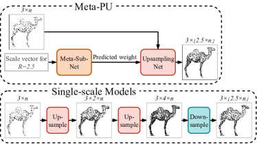
Figure 1: Arbitrary-scale model Meta-PU vs. the single-scale models over the example scale $R=2.5$. The existing single-scale models first need to scale to a larger integer scale (e.g., 4x), then use a downsample algorithm to achieve the noninteger scale of 2.5x.

However, all existing point cloud upsampling networks only consider certain integer scale factors (e.g., 2x). They regard the upsampling of different scale factors as independent tasks. Thus, a specific model for each scale factor has to be trained, limiting the use of these methods in real-world scenarios where different scale factors are needed to fit different densities of raw point clouds. Some works [6, 7] suggests to achieve larger scales through iterative upsampling (e.g., upsampling 4x by running the 2x model twice). However, this repeated computation is time-consuming, and upsampling of non-integer factors still cannot be achieved (e.g., 2.5x with single-scale models), as depicted in Fig. 1.

In real-world scenarios, it is very common and necessary to upsample raw point clouds into various user-customized densities for mesh reconstruction, point cloud processing, or other needs. Thus, an efficient method for upsampling arbitrary scale factors is desired to solve the aforementioned drawbacks in the existing methods. However, it is not easy for vanilla neural networks. Their behavior is fixed once trained because of the deterministic learned weights, so it is not straightforward to let the network handle the arbitrary scale factor on the fly.

Motivated by the development of meta-learning [8, 9] and the latest image super-resolution method [10], we propose an efficient and novel network called “Meta-PU” for point upsampling of arbitrary scale factors. By incorporating one extra cheap meta-subnetwork as the controller, Meta-PU can dynamically change its behavior during runtime depending on the desired scale factor. Compared with storing the weights for individual scale factors, storing the meta-subnetwork is more convenient and flexible.

Specifically, the backbone of Meta-PU is based on a graph convolutional network (GCN), consisting of several residual graph convolutional (RGC) blocks to extract the feature representation of each point as well as relationships to their nearest neighbors. And the meta-subnetwork is trained to generate weights for the meta-RGC block given the input of a scale factor. Then, the meta-convolution uses these weights to extract features that are adaptively tailored to the scale factor. Following several RGC blocks, a farthest sampling block is further added to output an arbitrary number of points. In this way, different scale factors can be trained simultaneously with a single model. At the inference stage, when users specify an upsampling scale factor, the meta-subnetwork will dynamically change the behavior of the meta-RGC block by adapting its weights and outputs the corresponding upsampling results.

To demonstrate the effectiveness and flexibility of our method, we compare it with several strong baseline methods. The comparison shows that our method can even achieve SOTA performances for specific single scale factors while supporting arbitrary-scale upsampling for the first time. In other words, our approach is both stronger and more flexible than the SOTA approaches. To better understand the underlying working principle and broader applications, we further provide a comprehensive analysis from different perspectives.

In summary, our contribution is three-fold:

• We propose the first point cloud upsampling network that supports arbitrary scale factors (including noninteger factors), via a meta-learning approach.

• We show that jointly training multiple scale factors with one model improves performance. Our arbitrary-scale model even achieves better results at each specific scale than the single-scale counterpart.

• We evaluate our method on multiple benchmark datasets and demonstrate that Meta-PU advances state-of-the-art performance.

2 Related Work

Optimization-based upsampling. Point cloud upsampling is formulated as an optimization problem in early work. A pioneering solution proposed by Alexa et al. [1] constructs a Voronoi diagram on the surface and then inserts points at the vertices. Lipman et al. [11] designed a novel locally optimal projection operator for point resampling and surface reconstruction based on $L_{1}$ median, which is robust to noise outliers. Later Huang et al. [2] improved the locally optimal projection operator to enable edge-aware point set upsampling. Wu et al. [3] employed a joint optimization method for the inner points and surface points defined in their new point set representation. However, most of these methods have a strong a priori assumption (e.g., a reasonable normal estimation or a smooth surface in the local geometry). Thus, they may easily suffer from complex and massive point cloud data.

Deep-learning-based upsampling. Recently, deep learning has become a powerful tool for extracting features directly from point cloud data in a data-driven way. Qi et al. firstly propose PointNet [12] and PointNet++ [13] for extracting multi-level features from point sets. Based on these flexible feature extractors, deep neural networks have been applied to many point cloud tasks, such as those in [14, 15, 16]. As for point cloud upsampling, Yu et al. [4] presented a point cloud upsampling neural network operating on the patch level and made it possible to directly input a high-resolution point cloud. Then, Yu et al. developed EC-Net [17] to improve the quality of the upsampled point cloud using an edge-aware joint learning strategy. Wang et al. proposed a progressive point set upsampling network [5] to suppress noise further and preserve the details of the upsampled point cloud. Moreover, different frameworks, such as the generative adversarial network (GAN) [18] and the graph convolutional network(GCN) [19], have attracted researchers’ attention for handling point cloud upsampling. Li et al. proposed the PU-GAN [6] by formulating a GAN framework to obtain more uniformly distributed point cloud results. Wu et al. proposed AR-GCN [7] to make the first attempt to model point cloud upsampling into a GCN. However, these networks are only designed for upsampling a fixed scale factor. When different upsampling scales are required in practical applications, multiple models have to be retrained. Unlike their methods, Meta-PU supports upsampling point clouds for arbitrary scale factors, by employing meta-learning to predict weights of the network and dynamically change behavior for each scale factor.

Meta-learning. Meta-learning, or learning to learn, refers to learning by observing the performance of different machine learning methods on various learning tasks. It is normally a two-level model: a meta-level model performed across tasks, and a base-level model acting within each task. The early meta-learning approach is primarily used in few-shot/zero-shot learning, and transfer learning [20, 21]. Recent works have also applied meta-learning to various tasks and achieved state-of-the-art results in object detection [22], instance segmentation [23], image super-resolution [10], image smoothing [8, 9, 24], network pruning[25], etc. A more comprehensive survey of meta-learning can be found in [26]. Among these works, meta-SR [10], which learns the weights of the network for arbitrary-scale image super-resolution, is closely related to ours. However, it cannot be applied to our task. The main reason is that the target of meta-SR is images with a regular grid structure, whereas our target includes much more challenging irregular and orderless point clouds. For regular grid-based images, since the correspondence between each output pixel and the corresponding input pixel is pre-determined, meta-SR can directly use relative offset information to regress the local upsampling weights. However, no such correspondence exists for point clouds. Therefore, we resort to using the meta-subnetwork together with the farthest sampling block. The meta-subnetwork is responsible for adaptively tailoring the point features of a specific scale factor by dynamically adjusting the weights of the RGC block, while the sampling block is responsible for sampling a particular number of points.

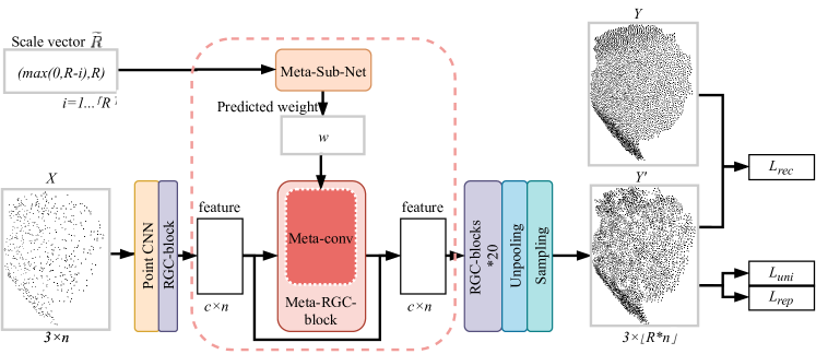
Figure 2: Overview of Meta-PU. Given a sparse input point cloud $X$ of $n$ points and a scale factor $R$, Meta-PU generates denser point cloud $Y^{\prime}$ with $\left\lfloor R\times n\right\rfloor$ points. A compound loss function is employed to encourage $Y^{\prime}$ to lie uniformly on the underlying surface of target $Y$. The pink box is the core part of Meta-PU. The meta-subnetwork takes scale factor $R$ as input and outputs the weight tensor $\mathbf{v}_{weight}$ for convolutional kernels in the meta-RGC block, to adapt the feature extraction to different upscales.

3 Method

In this section, we define the task of arbitrary-scale point cloud upsampling. Then we introduce the proposed Meta-PU in detail.

3.1 Arbitrary-scale Point Cloud Upsampling

Given a sparse and unordered point set $X=\left\{p_{i}\right\}_{i=1}^{n}$ of $n$ points, and with a scale factor $R$, the task of arbitrary-scale point cloud upsampling is to generate a dense point set $Y=\left\{p_{i}\right\}_{i=1}^{N}$ of $N=\left\lfloor R\times n\right\rfloor$ points. It is worth noting that $R$ is not necessarily an integer, and theoretically, $N$ can be any positive integer greater than $n$. The output $Y$ does not necessarily include points in $X$. In addition, $X$ may not be uniformly distributed. In order to meet the needs of practical applications, we need the upsampled point cloud to satisfy the following two constraints. Firstly, each point of $Y$ lies on the underlying geometry surface described by $X$. Secondly, the distribution of output points should be smooth and uniform, for any scale factor $R$ or input point number $n$.

3.2 Meta-PU

Overview. The backbone upsampling network contains five basic modules distinguished by different colors in Fig. 2. The input point cloud first goes through a point convolutional neural network (CNN) and several RGC blocks to extract features for each centroid and its neighbors. Among these RGC blocks, the meta-RGC block is special. The meta-RGC block weights are dynamically generated by a meta-sub-network given the input of $R$. Thus the features extracted by this meta-RGC block are tailored to the given scale factor. After the RGC blocks, an unpooling layer is followed to output $\left\lfloor R_{max}\times n\right\rfloor$ points, where $R_{max}$ denotes the maximum scale factor supported by our network, and $R_{max}=16$ by default. Afterward, the farthest sampling block is adopted to sample $N$ points from $\left\lfloor R_{max}\times n\right\rfloor$ points as the final output, which is constrained by a compound loss function. In the following section, we elaborate on the detailed structure of each block in Meta-PU, and the training loss.

Point CNN. The point CNN is a simple structure on the spatial domain to extract features from the input point cloud $X$. In detail, for each point $p\in X$ with shape $1\times 3$, we first group its $k$ nearest neighbors with shape $k\times 3$, and then feed them into a series of point-wise convolutions ($k\times c$) followed by a max-pooling layer to obtain $1\times c$ features, where $c$ is the channel number of point cloud feature. Thus, the output feature $F_{out}$ is a tensor of shape $n\times c$. Recursively applied convolution reaches a wider receptive field representing more information, whereas the maximum pooling layer aggregates information from all points in the previous layer. In our implementation, we set $k=8$, and $c=128$ and the number of convolutional layers is $3$.

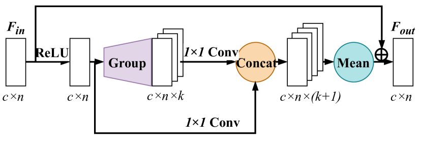
(a) RGC block

(b) Meta-RGC block

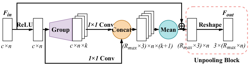
(c) Unpooling block

Figure 3: Structure of RGC block (a), meta-RGC block (b) and unpooling block (c). Both RGC and meta-RGC blocks convolve centroid features and neighborhood features, respectively. In the meta-RGC block, the weights of its convolutional layers are dynamically predicted based on the scale factor $R$. The unpooling block follows the last RGC block.

RGC Block. As shown in Fig. 3(a), the RGC block contains several graph convolutional layers and residual skip-connections, which is inspired from [7]. It takes the feature tensor $F_{in}$ as input and outputs $F_{out}$ of the same shape $n\times c$ as $F_{in}$.

The graph convolution in the RGC block is defined on a graph $\mathrm{G}=(V,\varepsilon)$, where $V$ denotes the node set and $\varepsilon$ denotes the corresponding adjacency matrix. The graph convolution is formulated as follows:

$$f_{out}^{p} ={\omega}_{0}\ast f_{in}^{p}+{\omega}_{1}\ast\Sigma_{q\in N(p)}f_{in}^{q},\forall p\in V$$ (1)

where $f_{in}^{p}$ denotes the input feature of vertex $p$, and $f_{out}^{p}$ represents the output feature of vertex $p$ after graph convolution, where ${\omega}$ is the learn-able parameters and $\ast$ denotes the point-wise convolutional operation.

The core idea of the RGC block is to separately operate the convolution on the central-point feature and neighbor feature, as illustrated in Fig. 3(b). For the neighbor features, they are grouped with the $k$ nearest neighbors of the input point cloud $x$ and then go through a $1\times 1$ graph convolution. The central-point features are convolved separately from those of the neighbors and then are concatenated with the neighbors’ features. Moreover, residual skip-connections are introduced to address the vanishing gradient and slow convergence problems. In our implementation, we set $k=8,c=128$, and a total of 22 RGC blocks are used. Among them, the second one is a special meta-RGC block, which is described in detail next.

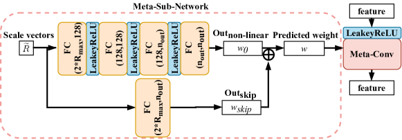
Figure 4: Structure of the meta-subnetwork. The meta-subnetwork inside the pink box predicts weights for convolutional layers in the meta-RGC block.

Meta-RGC Block and Meta-subnetwork. To solve the arbitrary-scale point cloud upsampling problem with a single model, we propose a meta-RGC block, which is the core part of Meta-PU. The meta-RGC block is similar to a normal RGC block, but the graph convolutional weights are dynamically predicted, depending on the given scale factor $R$. Instead of feeding $R$ directly into the meta-RGC block, we create a scale vector $\widetilde{R}=\{max(0,R-i),R\}_{i=1...\lceil R\rceil)}$ as the input and fill the rest with $\{-1,-1\}$ to achieve the size $2*R_{max}$. The philosophy behind this design is indeed inspired by meta-SR [10]. More specifically, because each input point is essentially transformed into a group of output points, $\{max(0,R-i),R\}$ can serve as the location identifier to guide the point processing network to differentiate the new $i-$th point from other points generated by the same input seed point.

The meta convolution is formulated as follows:

$$f_{out}^{p} ={\varphi}\left(\widetilde{R};{\theta}_{0}\right)\ast f_{in}^{p}+{\varphi}\left(\widetilde{R};{\theta}_{1}\right)\ast\Sigma_{q\in N(p)}f_{in}^{q},\forall p\in V$$ (2)

where the convolution weights are predicted by the meta-subnetwork ${\varphi}(.)$ taking the scale vector $\widetilde{R}$ as input. Please note we have two branches of meta-convolution, as shown in Fig. 3(b). One branch is for the feature of the center point $p$, and the other is for the feature of the neighbors defined by the adjacency matrix $\varepsilon$. Since there is no pre-defined adjacency matrix $\varepsilon$ for point clouds, we define it as $N(p)$, the $k$ nearest neighbors of $p$. The convolution weights of these two branches are generated by two meta-subnetworks with the parameters ${\theta}_{i}$ respectively.

Each meta-subnetwork for meta-convolution comprises five fully-connected (FC) layers [27] and several activation layers as shown in Fig.4. In the forward pass, the first FC layer takes the scale vector created from $R$ as input, and obtains a vector of $c_{hidden}$ entries. After the activation function, the second FC layer produces output of the same size as the input. Following the activation function, the input of the third FC layer is the $c_{hidden}$-entry encoding, and its output has length $c_{in}\times c_{out}\times l\times l$. Next, the fourth FC layer outputs a vector $w_{0}$ with the same shape as its input. Unlike the previous four concatenated layers, the last FC layer serves as a skip-connection that obtains output $w_{skip}$ of shape $c_{in}\times c_{out}\times l\times l$ directly from $2*R_{max}$. The two outputs $w_{0},w_{skip}$ are added and then reshaped to $(c_{in},c_{out},l,l)$ as the weight matrix $w$ for meta-convolution. We set $c_{out}=c_{in}=128$ and $c_{hidden}=128$. The $l$ represents the kernel size of the convolution, which is set to $1$ in our implementation. In the backward pass, instead of directly updating the weight matrix of the convolution, we calculate the gradients of the meta-subnetwork, with respect to the weights of the FC layers. The gradient of the meta-subnetwork can be naturally calculated by the Chain Rule to be trained end-to-end.

The meta-RGC block with dynamic weights predicted by the meta-subnetwork is necessary for the arbitrary-scale upsampling task because the upsampled point cloud $iR$-th to $(i+1)R$-th points are generated directly based on the features of the $i$-th input point and its nearest neighbors extracted via RGC blocks. The point locations in the output of different scale factors have to be different, to ensure that the uniformity of the upsampled points can cover the underlying surface. Therefore, the embedding features must be adaptively adjusted according to the scale factors. Therefore adaptive adjustment of the embedding features according to the scale factor is necessary. This adjustment is much better than mere upsampling to $R_{max}$ times and then performing the downsample. The experiments in Section 4.5 are designed to prove this.

The unpooling block takes point cloud $X$ and corresponding features $F_{in}$ as input. It is an RGC-based structure, while the output channels of the convolutional layers are set to $R_{max}\times 3$. Specifically, for feature $F_{in}$ of shape $n\times c$, it is transformed to a tensor of size $n\times(R_{max}\times 3)$, subsequently reshaped to $n\times R_{max}\times 3$, denoted as $T_{out}$. As a residual block, similar to the residual connection of the input and output features in the RGC block, we introduce a skip connection between points. Thus, the tensor $T_{out}$ is then point-wisely added to $X$ to produce the output $Y^{\prime}_{max}$ of shape $n\times R_{max}\times 3$. Note that the “add” operation naturally expands $x$ to $R_{max}$ copies in a broadcast manner.

The farthest sampling block performs a farthest sampling strategy to retain $Y^{\prime}$ with $n\times R$ points from $Y^{\prime}_{max}$ with $\left\lfloor R_{max}\times n\right\rfloor$. The advantages are two-fold. First, the farthest sampling can sample an arbitrary number of points from the input point set, which helps obtain the required number of points as output. Second, since the farthest sampling iteratively constructs a point set with the farthest point-wise distance according to the Euclidean distance from a global perspective, this step further enhances the uniformity of the point set distribution.

3.3 Loss Function

For end-to-end training of Meta-PU, we adopt a compound loss with both reconstruction terms $\mathcal{L}_{\mathrm{rec}}$ and uniform terms $\mathcal{L}_{\mathrm{uni}},\mathcal{L}_{\mathrm{rep}}$:

$$\mathcal{L}=\lambda_{\mathrm{rec}}\mathcal{L}_{\mathrm{rec}}+\lambda_{\mathrm{uni}}\mathcal{L}_{\mathrm{uni}}+\lambda_{\mathrm{rep}}\mathcal{L}_{\mathrm{rep}}$$ (3)

The latter two terms aim at encouraging the uniformity of the generated point cloud and improving the visual quality.

Repulsion loss [4] $\mathcal{L}_{\mathrm{rep}}$ is represented as follows:

$$\mathcal{L}_{rep}=\sum_{i=0}^{N}\sum_{i^{\prime}\in K(i)}\eta\left(\left\|p_{i^{\prime}}-p_{i}\right\|\right)w\left(\left\|p_{i^{\prime}}-p_{i}\right\|\right)$$ (4)

where $N$ is the number of output points, $K(i)$ is the index set of the k-nearest neighbors of point $p_{i}$ in output point cloud $Y^{\prime}$, $\eta(r)=-r$ is the repulsion term, and $w(r)=e^{-r^{2}/h^{2}}$.

Uniform loss The term [6] $\mathcal{L}_{\mathrm{uni}}$ comprises two parts: $U_{\text{imbalance }}$ accounting for global uniformity, and $U_{\text{clutter }}$ accounting for the local uniformity.

$$\mathcal{L}_{\mathrm{uni}}=\sum_{j=1}^{M}U_{\mathrm{imbalance}}\left(S_{j}\right)\cdot U_{\mathrm{clutter}}\left(S_{j}\right)$$ (5)

where $S_{j},j=1..M$ refers to the ball queried point subsets with radius $r_{d}$ and centered at $M$ seed points farthest sampled from $Y^{\prime}$.

$$U_{\text{imbalance }}\left(S_{j}\right)=\frac{\left(\left|S_{j}\right|-\hat{n}\right)^{2}}{\hat{n}}$$

where $\hat{n}=\hat{N}\times r^{2}_{d}$, referring to the expected number of points in $S_{j}$. Note that, the imbalance term is not differentiable, which acts as a weight for the following clutter term.

$$U_{\text{clutter }}\left(S_{j}\right)=\sum_{k=1}^{\left|S_{j}\right|}\frac{\left(d_{j,k}-\hat{d}\right)^{2}}{\hat{d}}$$

where $d_{j,k}$ is the point-to-neighbor distance of the $k$-th point in $S_{j}$, while $\hat{d}=\sqrt{\frac{2\pi r_{d}^{2}}{\left|S_{j}\right|\sqrt{3}}}$ denotes the expected distance.

Un-biased Sinkhorn divergences [28] are proposed by us as the reconstruction loss, to encourage the distribution of generated points to lie on the underlying mesh surface. It is the interpolation between the Wasserstein distance and kernel distance. The Sinkhorn divergences between output $Y^{\prime}$ and the groundtruth $Y$ can be formulated as follows:

$$\mathcal{L}_{\mathrm{rec}} =\mathrm{S}_{\varepsilon}(Y,Y^{\prime})=\mathrm{OT}_{\varepsilon}(Y,Y^{\prime})$$ (6)

$$-\frac{1}{2}\mathrm{OT}_{\varepsilon}(Y,Y)-\frac{1}{2}\mathrm{OT}_{\varepsilon}(Y^{\prime},Y^{\prime})$$

where $\varepsilon$ is the regularization parameter, and

$$\mathrm{OT}_{\varepsilon}(Y,Y^{\prime})\stackrel{{\scriptstyle\text{ def. }}}{{=}}\min_{\pi_{1}=Y,\pi_{2}=Y^{\prime}}\int_{\mathcal{X}^{2}}\mathrm{C}\mathrm{d}\pi+\varepsilon\mathrm{KL}(\pi\mid Y\otimes Y^{\prime})$$

with a cost function on the feature space $\mathcal{X}\subset\mathbb{R}^{\mathrm{D}}$ of dimension $\mathrm{D}$ as follows:

$$C(x,y)=\frac{1}{2}\|x-y\|_{2}^{2}$$ (7)

and where optimization is performed over the coupling measures $\pi\in\mathcal{M}_{1}^{+}\left(\mathcal{X}^{2}\right)$ as $\left(\pi_{1},\pi_{2}\right)$ denotes the $\pi$’s two marginal.

3.4 Variable-scale Training Strategy

In the training process of most existing single-scale point cloud upsampling methods, each model is trained with one scale factor. However, because the scale factor varies in our arbitrary-scale upsampling task, we need to design a variable-scale training scheme to train all factors jointly. We first sampled all factors from the range of $1.1$ to $R_{max}$ with a stride of $0.1$, and put them in set $\mathcal{S}_{R}$. For each epoch, a scale factor, say $R$, is randomly sampled from $\mathcal{S}_{R}$, and this factor is shared in a batch. To avoid overfitting, we also perform a series of data augmentation: rotation, random scaling, shifting, jittering, and perturbation with low probability.

4 Experiments

4.1 Datasets and Metrics

Dataset. For training and testing, we utilize the same dataset adopted by PU-Net [4] and AR-GCN [7]. This dataset contains $60$ different models from the Visionair repository. Following the protocol in the above two works, $40$ models are used for training and the rest $20$ models are used for testing.

For training, 100 patches are extracted from each model, thus we have a total of $40,000$ patches. We uniformly sample $N$ points using Poisson disk sampling from each patch as the ground truth, and non-uniformly sample $n$ points from the ground truth as input, where $n=\left\lfloor n_{max}\times\frac{1}{R}\right\rfloor$, and $N=R\times\left\lfloor n_{max}\times\frac{1}{R}\right\rfloor$, corresponding to the scale factor $R$. Moreover, we set $n_{max}=4096$ as the maximum number of points in our training. For testing, we use the whole model instead of the patch. The sampling process of the ground truth and input is similar to that in training. But constrained by the GPU memory limit, we set different numbers of input points for different scale factors, i.e. $5000$ for $R<=4$, $4000$ for $4<R<=6$, $3000$ for $6<R<=12$, and $2500$ for $R>12$.

TABLE I: Experiments of quantitative comparisons. Single-scale models (including AR-GCN and PU-GAN) trained with each specific scale factor (top two rows) vs. the naive approach of arbitrary-scale upsampling (rows 3 to 5) vs. our full model (last row). The NUC scores are tested with $p=0.8\%$.

Methods\Scales	2x						4x
	CD	EMD	F-score	NUC	mean	std	CD	EMD	F-score	NUC	mean	std
AR-GCN	-	-	-	-	-	-	0.0086	0.018	70.09%	0.339	0.0029	0.0033
PU-GAN	0.016	0.0090	32.17%	0.249	0.012	0.015	0.0097	0.016	69.75%	0.202	0.0030	0.0031
AR-GCN(x16)	0.015	0.023	30.14%	0.307	0.0089	0.014	0.012	0.041	45.34%	0.256	0.0081	0.0096
+random-sampling
AR-GCN(x16)	0.014	0.012	33.52%	0.227	0.0088	0.011	0.011	0.018	52.67%	0.318	0.0072	0.0092
+farthest-sampling
AR-GCN(x16)	0.015	0.013	36.98%	0.273	0.0067	0.0082	0.013	0.013	54.05%	0.288	0.0066	0.0080
+disk-sampling
ours	0.010	0.0049	53.20%	0.127	0.0023	0.0029	0.0080	0.0078	74.05%	0.192	0.0022	0.0027

Methods\Scales	6x						9x						16x
	CD	EMD	F-score	NUC	mean	std	CD	EMD	F-score	NUC	mean	std	CD	EMD	F-score	NUC	mean	std
AR-GCN	-	-	-	-	-	-	0.0081	0.022	74.63%	0.344	0.0034	0.0044	0.0085	0.023	75.33	0.522	0.0029	0.0037
PU-GAN	0.012	0.013	58.56%	0.287	0.011	0.018	0.0091	0.0085	70.61%	0.212	0.0047	0.0057	0.0092	0.022	70.79	0.431	0.0042	0.0041
AR-GCN(x16)	0.013	0.025	46.11%	0.309	0.0077	0.0099	0.011	0.039	48.80%	0.417	0.0080	0.0086	-	-	-	-	-	-
+random-sampling
AR-GCN(x16)	0.011	0.078	53.97%	2.808	0.0075	0.0085	0.011	0.015	53.89%	5.522	0.0081	0.0081	-	-	-	-	-	-
+farthest-sampling
AR-GCN(x16)	0.012	0.014	59.41%	0.293	0.0065	0.0079	0.011	0.014	62.70%	0.298	0.0065	0.0078	-	-	-	-	-	-
+disk-sampling
ours	0.0083	0.014	74.98%	0.267	0.0025	0.0030	0.0083	0.016	73.74%	0.274	0.0030	0.0034	0.0082	0.023	75.62	0.428	0.0029	0.0035

TABLE II: Quantitative comparisons with the EAR. The NUC scores are tested with $p=0.8\%$.

Methods	CD$\downarrow$	EMD$\downarrow$	F-score$\uparrow$	NUC$\downarrow$	mean$\downarrow$	std$\downarrow$
EAR (2x)	0.0113	0.0214	48.07%	0.747	0.0048	0.0113
Ours (2x)	0.010	0.0049	53.20%	0.127	0.0023	0.0029
EAR (4x)	0.0112	0.0176	51.26%	0.478	0.0074	0.0137
Ours (4x)	0.0080	0.0078	74.05%	0.192	0.0022	0.0027
EAR (6x)	0.0120	0.0184	52.26%	0.421	0.0085	0.0145
Ours (6x)	0.0083	0.014	74.98%	0.267	0.0025	0.0030
EAR (9x)	0.0119	0.0174	52.93%	0.442	0.0089	0.0140
Ours (9x)	0.0083	0.016	73.74%	0.274	0.0030	0.0034

Metrics. For a fair comparison, we employ several different popular metrics: Chamfer Distance (CD) and Earth Mover Distance (EMD) defined on the Euclidean distance are to measure the difference between predicted points $Y^{\prime}$ and ground-truth point cloud $Y$. The CD sums the square of the distance between each point and the nearest point in the other point set, then calculates the average for each point set. The EMD measures the minimum cost of turning one of the point sets into the other. For these two metrics, the lower, the better. We also report the F-score between $Y^{\prime}$ and $Y$ that defines the point cloud super-resolution as a classification problem as [7]. For this metric, larger is better. We employ the normalized uniformity coefficient (NUC)  [4] to evaluate the uniformity of $Y^{\prime}$ by directly comparing the output point cloud $Y^{\prime}$ with corresponding ground-truth meshes, and deviation mean and std to measure the difference between the output point cloud and ground-truth mesh. For these two metrics, smaller is better.

4.2 Implementation Details

We train the network for 60 epochs with a batch size of 18. Adam is adopted as the loss optimizer. The learning rate is initially set to 0.001 for FC layers and 0.0001 for convolutions and other parameters, which is decayed with a cosine annealing scheduler to $1e-5$. Parameters $\lambda_{\mathrm{rec}}$, $\lambda_{\mathrm{uni}}$ and $\lambda_{\mathrm{rep}}$ for the joint loss function are set to $1$, $0.001$ and $0.005$ respectively. Generally, the training takes less than seven hours on two Titan-XP GPUs.Theoretically, MetaPU supports any large scale, but we set the maximum scale to 16 due to the limitations of the computing resources and practical needs.

TABLE III: Quantitative comparisons with MPU. Our method obtains superior results under most metrics.

Method	CD	EMD	F-score	NUC with different p					Deviation(1e-2)		Time
				0.2%	0.4%	0.6%	0.8%	1.0%	mean	std
MPU(2x)	0.0097	0.0132	52.65%	0.317	0.271	0.252	0.241	0.234	0.21	0.30	5.16
ours(2x)	0.010	0.0049	53.20%	0.183	0.147	0.134	0.127	0.123	0.23	0.29	0.90
MPU(4x)	0.0086	0.012	73.16%	0.321	0.282	0.265	0.256	0.249	0.22	0.28	36.28
ours(4x)	0.0080	0.0078	74.05%	0.245	0.213	0.200	0.192	0.187	0.22	0.27	0.91
MPU(16x)	0.0078	0.023	76.35%	0.425	0.378	0.357	0.346	0.337	0.28	0.35	389.40
ours(16x)	0.0082	0.023	75.62%	0.555	0.482	0.448	0.428	0.414	0.29	0.35	0.50

TABLE IV: Comparison of the inference time.

Method	AR-GCN + Disk-sampling	PU-GAN + Disk-sampling	EAR	ours
Time(s)	10.28	10.06	351.10	0.79

4.3 Ablation Analysis

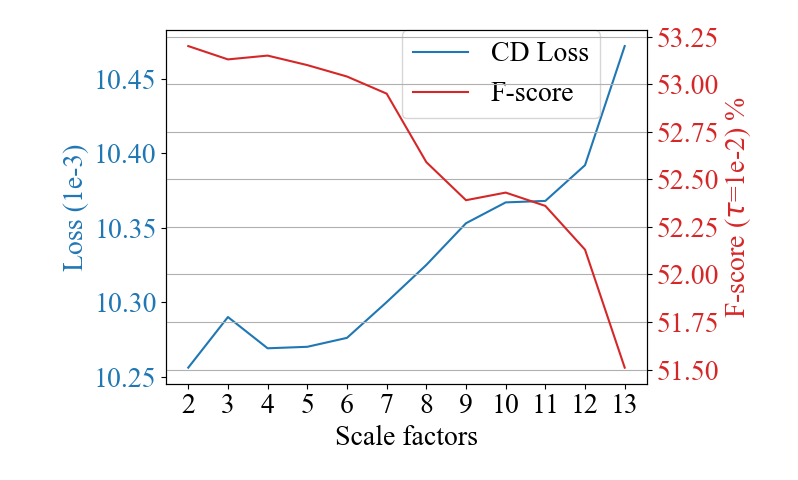
Figure 5: Ablation on the meta-RGC block. Meta-PU is applied to upsample the point clouds to 2x, but the weights of its meta-RGC block are generated with a different input scale factor $R$. $R=2$ achieves the best performance on both F-score and CD, which indicates our meta-RGC block adapts the convolutional weight appropriately to different scale factors.

4.4 Comparison with Single-scale Upsampling Methods

In this experiment, we compare Meta-PU with state-of-the-art single-scale upsampling methods, including PU-GAN [6] and AR-GCN [7], to upsample the sparse point cloud with scale factors $R\in[2,4,6,9,16]$. Their models are trained with the author-released code, and all settings are the same as stated in their papers. Since they are single-scale upsampling methods, for each scale factor, an individual model is trained. Due to the limitations of the two-stage upsampling strategy, AR-GCN can only be trained with the factors $4,9,16$, whereas PU-GAN can be trained with all four factors. Their performance is reported in the first two rows of Table I. We surprisingly observe that our arbitrary-upscale model even outperforms their single-scale models with most scale factors. Particularly, our model performs significantly better on the F-score, NUC, mean, and std metrics than other models, and is more stable on all scales. This may be because multiple joint training tasks of different scales can benefit each other, thus improving performance. In addition, Meta-PU needs to train only once for all testings, while others need to train multiple models, which is very inefficient.

4.5 Comparison with Naive Arbitrary-scale Upsampling Approaches

A naive approach to achieve arbitrary-scale upsampling is to first use a state-of-the-art single-scale model to upsample the cloud point to a large scale, and then downsample it to a specific smaller scale. We compare our method with this naive approach. Specifically, we choose AR-GCN [7] to upsample point clouds to 16x and then downsample them to 2x,4x,6x and 9x with the random sampling, disk sampling, and farthest sampling algorithms. The results are reported in 3-5th rows of Table I. We can see that random sampling gets the worst scores because it non-uniformly downsamples the points. In comparison, the more advanced sampling algorithms, including disk sampling and farthest sampling, perform better by considering uniformity. Our method is still superior to all of them because the result of a smaller scale factor in our method is not simply a subset of the large-factor one. In fact, Meta-PU can adaptively adjust the location of the output points to fit the underlying surface better and maintain uniformity according to different scale factors. This will be analyzed by the ablation study of the meta-RGC block in the next subsection. Moreover, compared to the strongest baseline (AR-GCN+disk-sampling), ours is 120 times faster (Table IV), because this advanced upsampling algorithm requiring mesh reconstruction is slow.

We also compare our method with the state-of-the-art optimization-based method EAR [29], which is also applicable to variable scales. The results of scale 2,4,6,9,16 are provided in Table II. It could be found that our method yields superior results under all metrics.

Further, we compare Meta-PU with the state-of-the-art multistep upsample method MPU [5] that recursively upsamples a point set, which is also applicable to scales of a power of 2,( e.g., 2,4,16). The results of scales 2,4,16 are provided in Table III. It can be found that our method obtains superior results under most metrics. In addition, we provide a comparison of inference times. The running time of our method is much less at all scales, demonstrating that our method is more efficient than the recursive approach.

4.6 Inference Time Comparison

In Table IV, we provide the comparison of the average inference time of all integer scales in (1,16]. Since Disk-sampling obtains the best performance as shown in Table I, it is employed in other single-scale baselines for arbitrary-scale upsampling. We also compare the inference time of ours with the optimization-based method EAR. The running time of our method is much less than all the compared methods. Specifically, the speed of a trivial single-scale baseline is dragged down by the bottleneck of disk-sampling. We also calculated the inference time of our model at the scales of 2,4,6,9, and 16 with 2500 points. We found no difference in inference time for different scales, demonstrating the stability of our method in terms of inference time.

4.7 Quantitative Metrics on Varying Scales

Fig. 6 shows the quantitative comparison results of the F-scores and CD loss for point cloud upsampling with different scales. It demonstrates that our method can support a wide range of scales, and that the performances on different scales are stable. We need to note that the lower F-score for small scales (e.g., 2) is because one fixed distance threshold is used in calculating the F-scores, causing the F-score to be relatively low when the point cloud is too sparse.

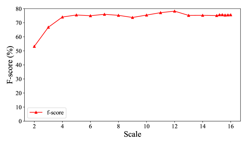
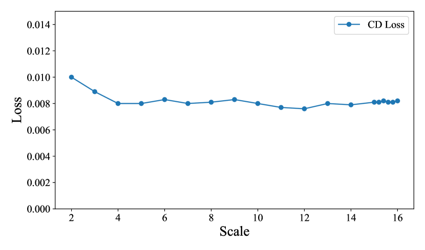
Figure 6: F-scores and CD losses of upsampling on different scales with Meta-PU. Our method performs stably on different scales.

TABLE V: Ablation on the meta-RGC block.

Methods\F-score	2x	4x	6x
Full-model	53.20	74.05	74.98
Replace Meta-RGC	52.33	73.08	74.09

Figure 7: Close up of the upsampling results with and without meta-RGC block; Greens: full model, Reds: w/o meta-RGC block.

Importance of the Meta-RGC Block. We design an experiment to evaluate the influence of the meta-RGC block quantitatively. We use Meta-PU to upsample point clouds to 2x, but the weights of the meta-RGC block are generated with different input $R$. We measure the average F-score and CD values on the testing set for different $R$, as plotted in Fig. 5. It can be observed that the best performance for both the F-score and CD is achieved when the input scale factor $R$ of the meta-RGC block equals the target upsampling scale $2$. This demonstrates the meta-RGC block adapting the convolution weight properly to different scale factors. Moreover, the meta-RGC block adaptation to various scale factors is the key to makeing the output points better fit the underlying surface and keep uniform. To demonstrate this, we respectively train the full model and our model where the meta-RGC block is replaced by normal RGC-block, and show the close up of some results in Fig.7. It is obvious that the results of our full model are more precise, sharper and cleaner, especially around key positions, such as corners. Also, we conducted an ablation study to replace the meta-RGC with normal RGC, while keeping all the other parts fixed. The results are shown in Table V. These results demonstrate the meta-RGC block adapts the convolutional weight properly to different scale factors and improves performance. Therefore, as we explained before, the performance improvements of our method mainly come from two aspects: the joint training of multiple scale factors with one model and the meta-RGC block.

Another important function of the meta-RGC block is enabling adaptive receptive fields for different scales, which is useful because large-scale upsampling typically takes sparser input and requires exploring long-range relationships between input points. To demonstrate this, we analyze the effective receptive fields. Specifically, we fix the model weights of Meta-PU and remove the farthest sampling block to eliminate its influence. Then, we test the model with the same inputs but different scale factors. In the common input, we randomly choose a point and find its closest output point in the results of each factor as the centroids. We mask out the gradients from all points except the centroid and propagate the gradients back to the input points. Only the input points whose gradient values are larger than $1\%$ of the maximum gradient value are considered within the receptive field of the center point. As shown in Fig. 8, the receptive field is dynamically increased with the larger input scale factor of the meta-RGC block.

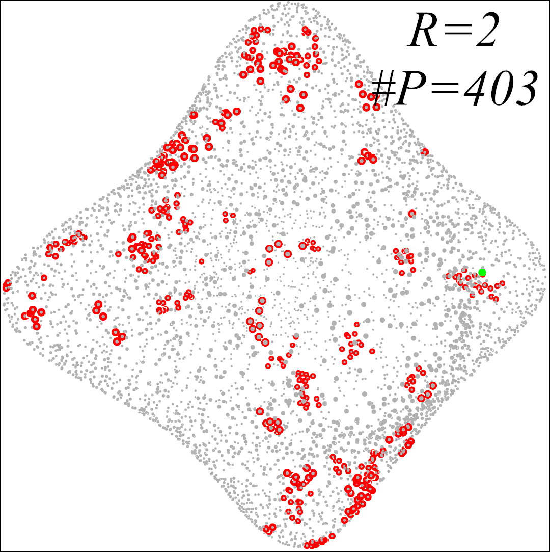
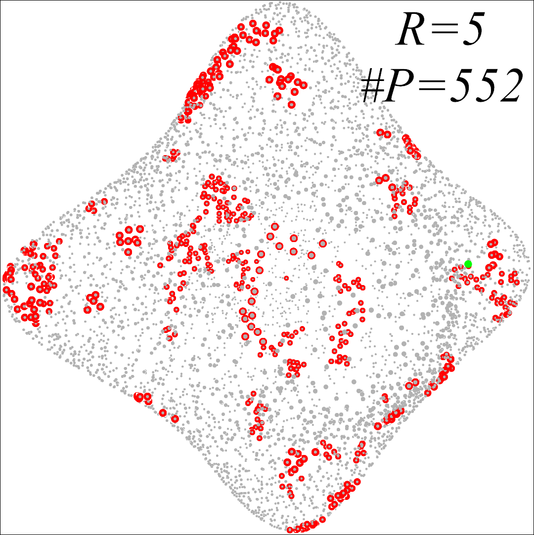
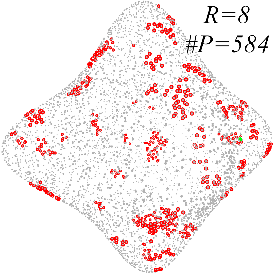
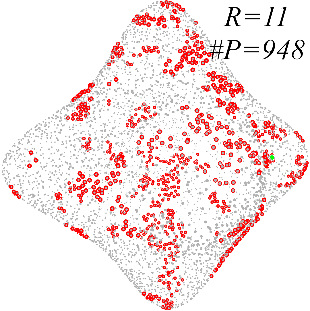
Figure 8: Visualizations of center points (Green), corresponding effective receptive fields (Red) in the input, and other points in the input (Gray). The scale factors are 2,5,8,11 from left to right. $\#P$ indicates the number of input points within the receptive field.

TABLE VI: Experiments on our specially designed scale tensor vs simply feeding the original scale factor. All models are tested with a scale factor of 4. Our specially designed scale tensor performs better.

Method	CD	EMD	F-score	NUC with different p					Deviation(1e-2)
				0.2%	0.4%	0.6%	0.8%	1.0%	mean	std
all-R	0.0081	0.0078	73.46%	0.250	0.216	0.202	0.194	0.189	0.23	0.28
ours	0.0080	0.0078	74.05%	0.245	0.213	0.200	0.192	0.187	0.22	0.27

Importance of Specially Designed Scale Tensor. In this ablation study, we aim to show the advantages of our designed scale tensor $\widetilde{R}$ with the location identifier over directly feeding $R$ into the meta-RGC block. In the first row of Table. VI, we fill the scale tensor with all $R$s and train the model with the same setting. We can observe that the model with the specially designed scale tensor performs better, because the location identifier in our scale tensor contains extra information to guide the network to better differentiate a group of points, generated by the same seed point, from each other.

TABLE VII: Experiments on our model with Sinkhorn loss vs. Chamfer Distance vs. GAN loss. All models are tested with a scale factor of 4.

Method	CD	EMD	F-score	NUC with different p					Deviation(1e-2)
				0.2%	0.4%	0.6%	0.8%	1.0%	mean	std
ours-CD	0.0090	0.0099	65.49%	0.256	0.230	0.218	0.211	0.206	0.47	0.51
with GAN-loss	0.0081	0.0081	73.69%	0.259	0.222	0.208	0.199	0.192	0.22	0.28
ours	0.0080	0.0078	74.05%	0.245	0.213	0.200	0.192	0.187	0.22	0.27

Ablation on Loss Terms. To validate our choice on the loss terms, we design two ablation experiments. In the first experiment, we replace the Sinkhorn loss with the CD distance in our method as [7] and report the performance (ours-CD) in Table VII. It clearly demonstrates the superiority of the Sinkhorn divergence reconstruction loss over CD. For example, the F-score using the Sinkhorn loss is about 7% better than that using the CD loss. Rather than just measuring the distance between every nearest point between two point sets in the CD loss, the Sinkhorn loss considers the joint probability between two point sets and encourages the distribution of the generated points to lie on the ground-truth mesh surface. In the second experiment, we add the GAN-loss to our full-model (with GAN-loss). The scores on 4x are reported in Table VII. We found the GAN loss does not further improve the performance of our model. Thus, we do not include it in our implementation.

TABLE VIII: Experiments on training Meta-PU with different upscale ranges $R_{max}$ and testing with scale factor $4$. Training with a wider range brings performance improvements.

Method	CD	EMD	F-score	NUC with different p					Deviation(1e-2)
				0.2%	0.4%	0.6%	0.8%	1.0%	mean	std
ours(max5)	0.0079	0.015	72.85%	0.386	0.341	0.324	0.314	0.305	0.20	0.22
ours(max9)	0.0081	0.011	73.39%	0.248	0.214	0.202	0.193	0.189	0.22	0.27
ours(max16)	0.0080	0.0078	74.05%	0.245	0.213	0.200	0.192	0.187	0.22	0.27

Ablation on Different Scale Ranges. To test the influence of the scale factor ranges in our method, we design an experiment comparing our model trained with different $R_{max}$ but all tested with $R=4$. The result is reported in Table VIII, in which we compare the results of the models trained with $R_{max}=5,9,16$. Generally, ours(max16) trained with the widest range performs the best, while ours(max9) are better than ours(max5). From this, we can conclude that upsampling tasks with scale factors have some shared properties that allow them to benefit from each other during joint training, further allowing the models to learn some common knowledge about upsampling as well.

TABLE IX: Quantitative results on SHREC15 with scale=4. The NUC scores are tested with $p=0.8\%$.

Methods	CD$\downarrow$	EMD$\downarrow$	F-score$\uparrow$	NUC$\downarrow$	mean$\downarrow$	std$\downarrow$
AR-GCN	0.0048	0.0127	94.04%	0.364	0.0018	0.0022
Ours	0.0045	0.0071	94.96%	0.197	0.0015	0.0016

4.8 Applications

In this section, we reveal the advantages of our method in different practical applications, including mesh reconstruction, point cloud classification, upsampling on real data, and upsampling with arbitrary input sizes or scales.

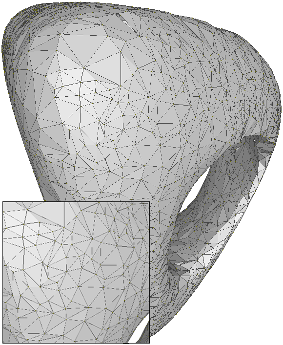
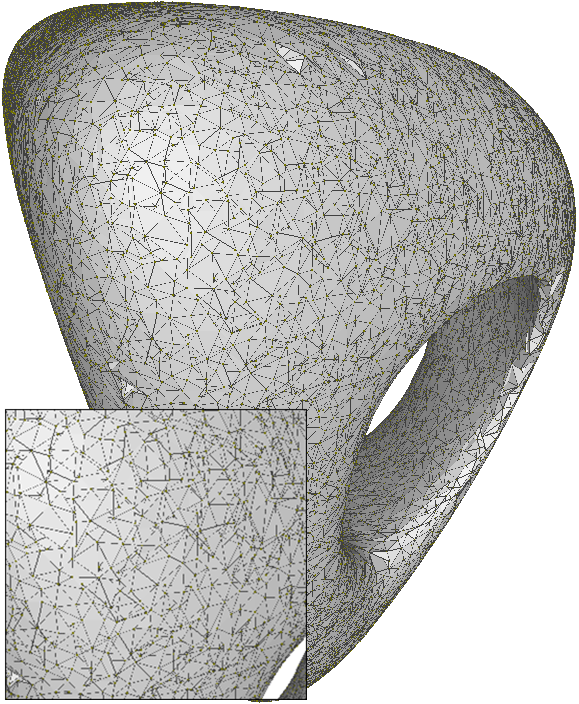
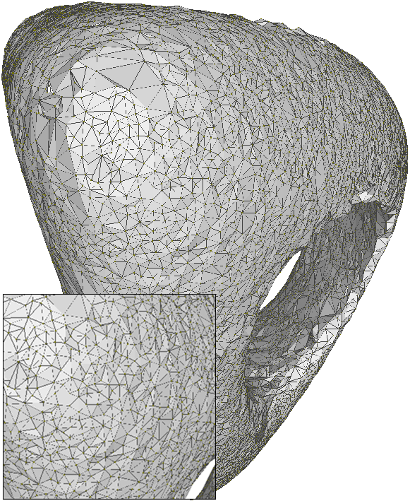
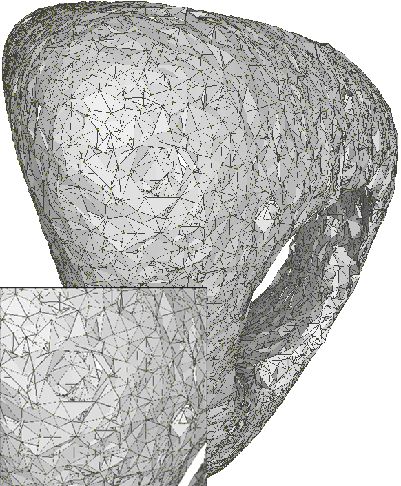
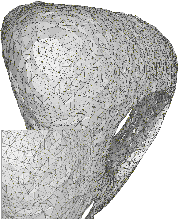
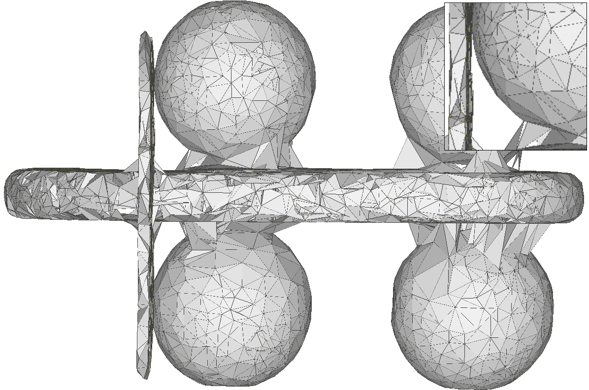
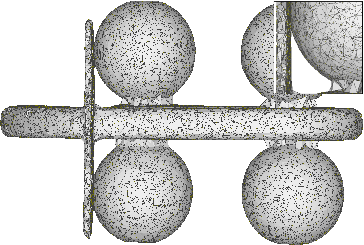
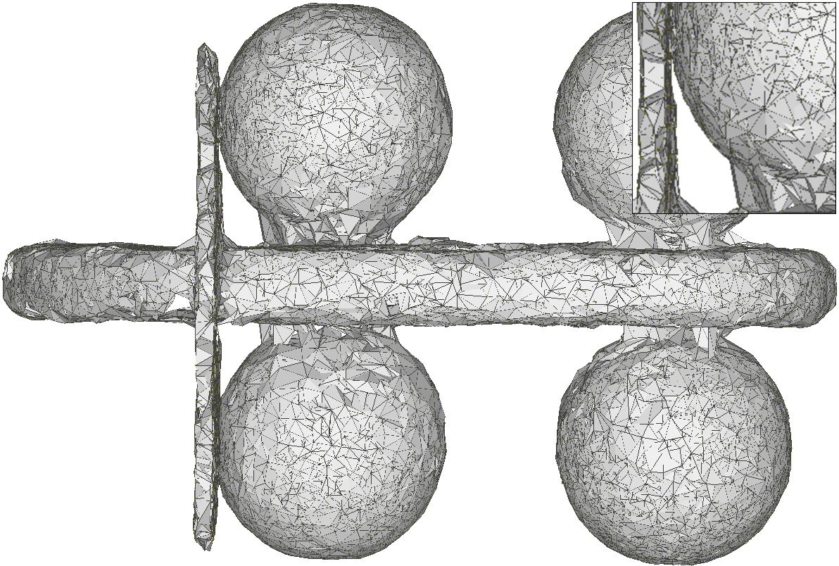
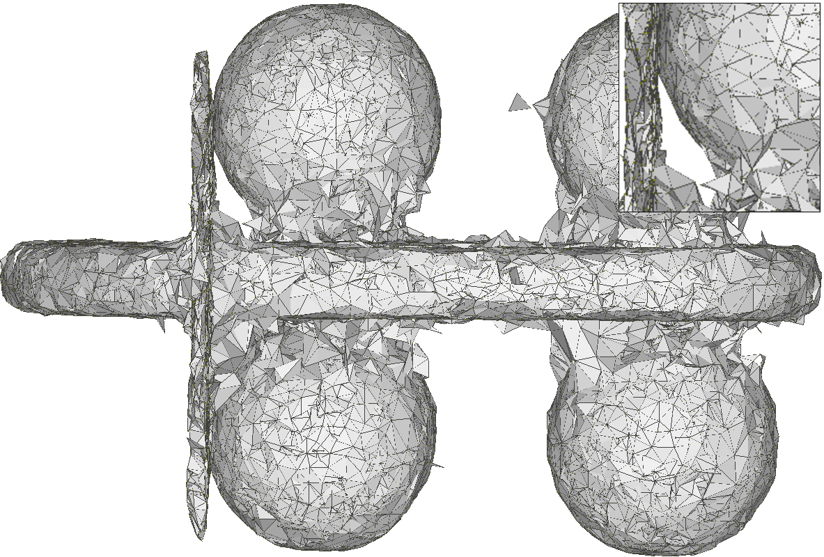
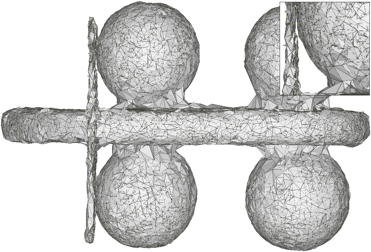
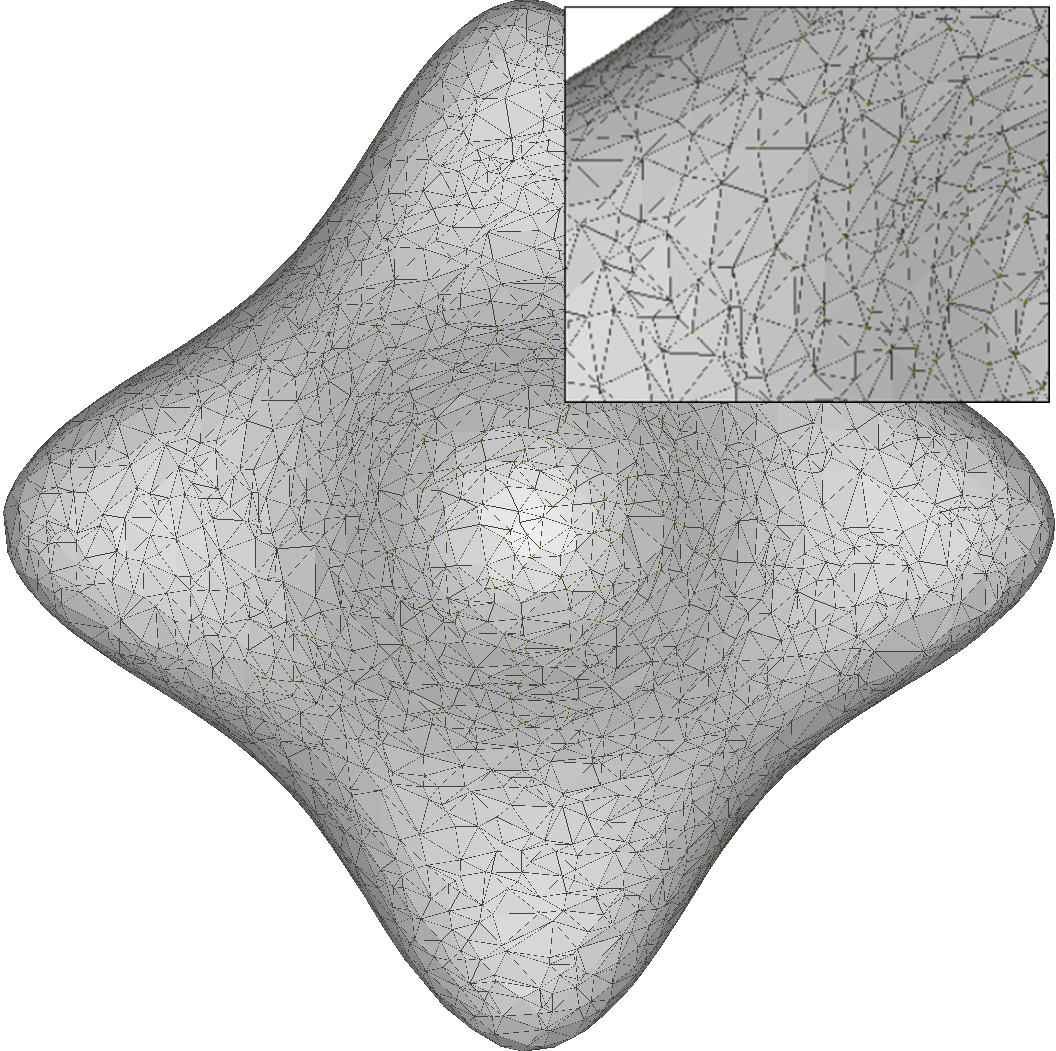
Input

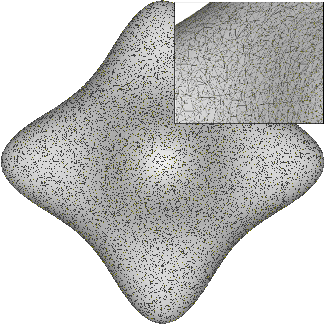
GT

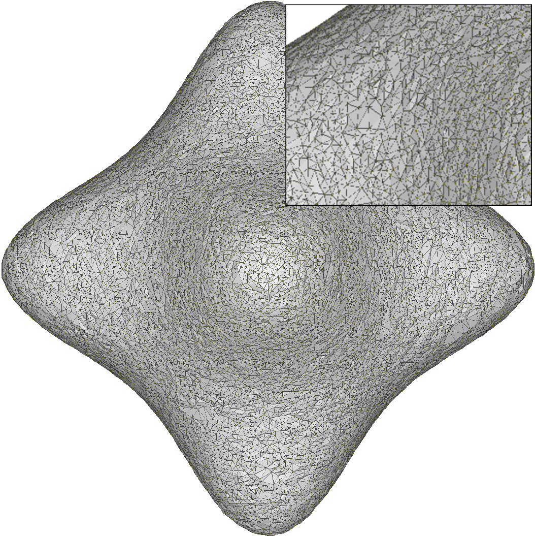
Ours

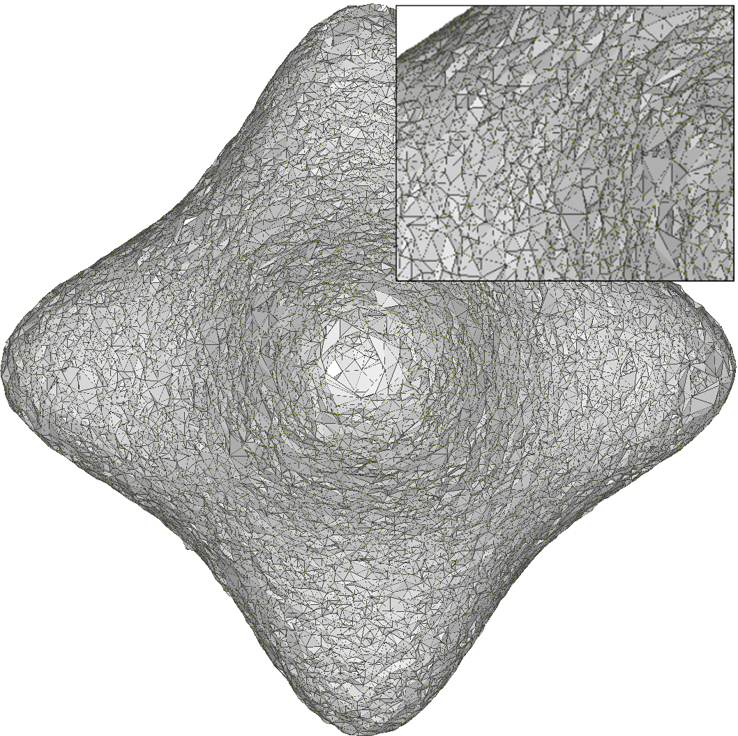
PU-GAN

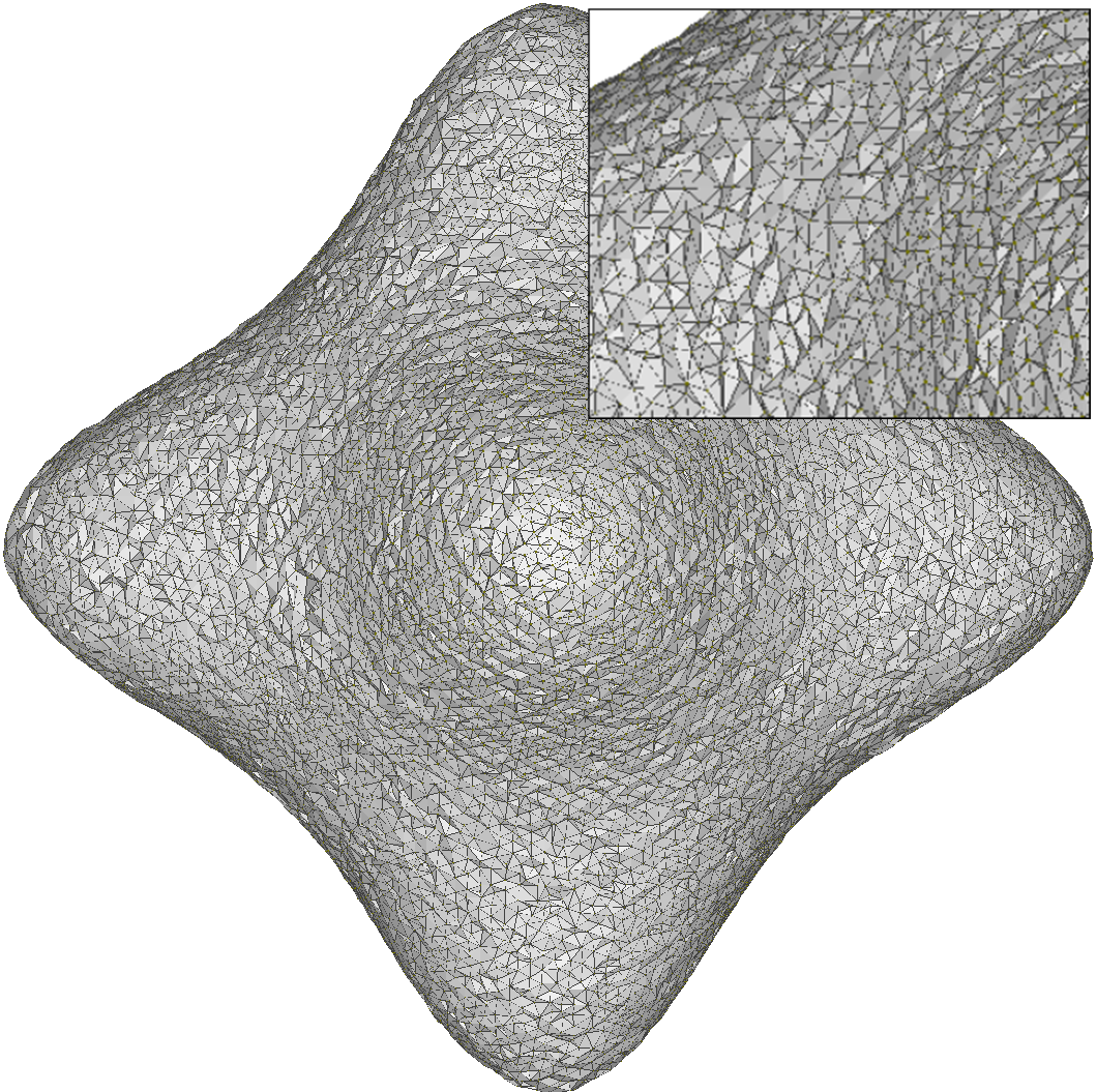
ARGCN

Figure 9: Results of the mesh reconstruction from 4x upsampled point cloud with ball pivoting.

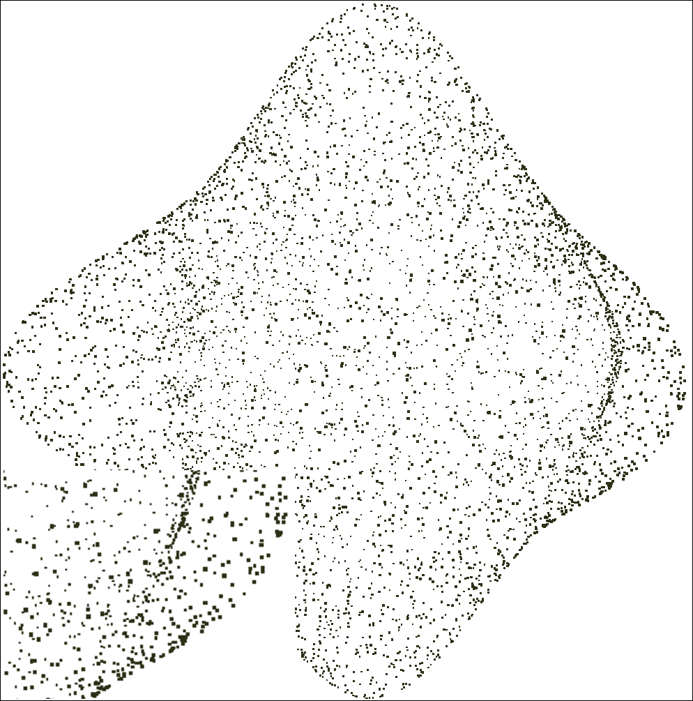
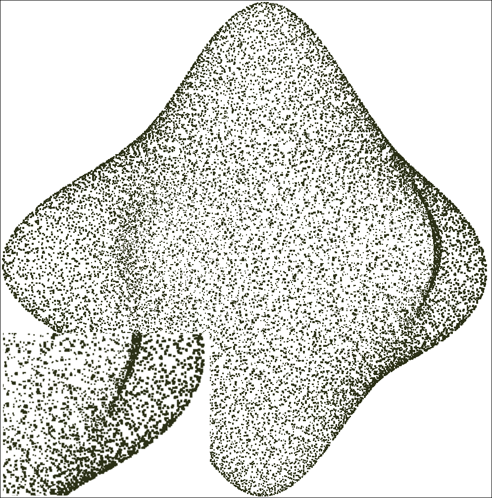
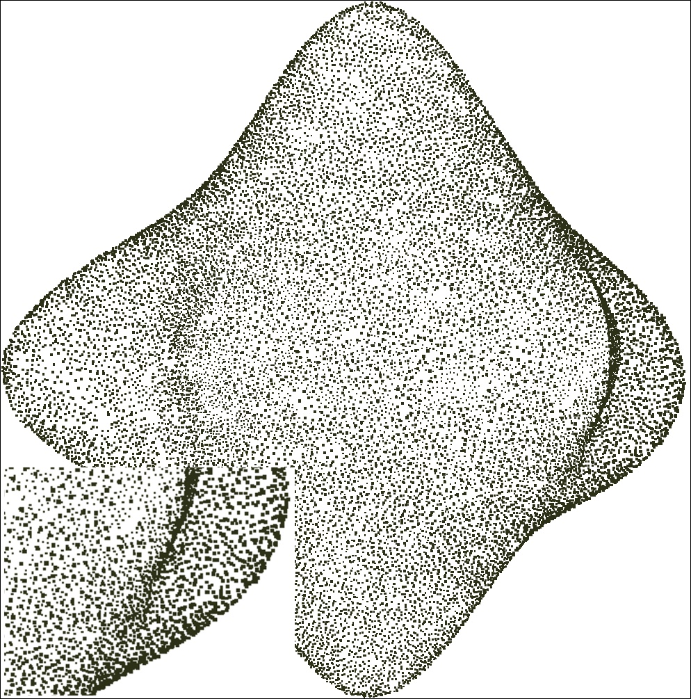
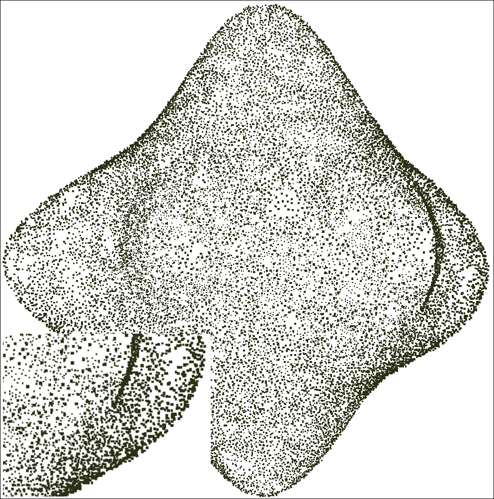
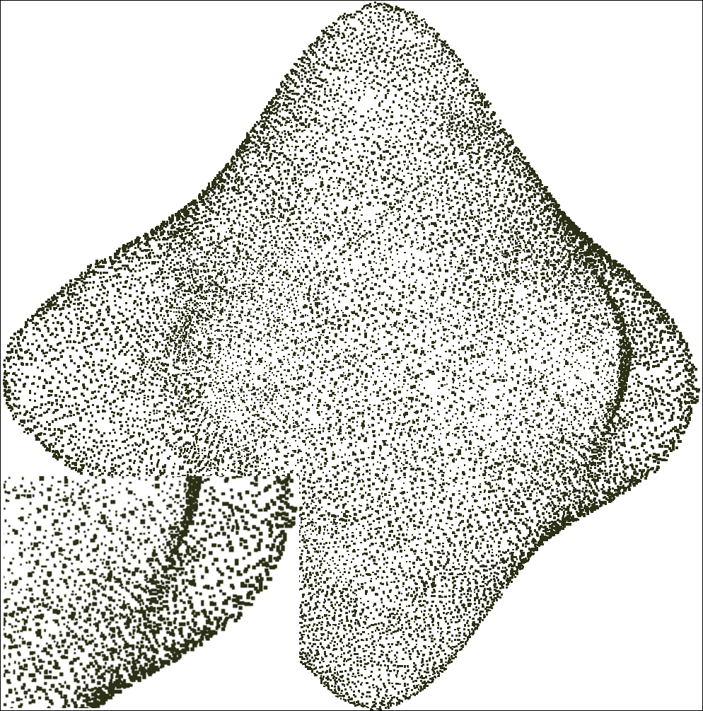
Input

GT

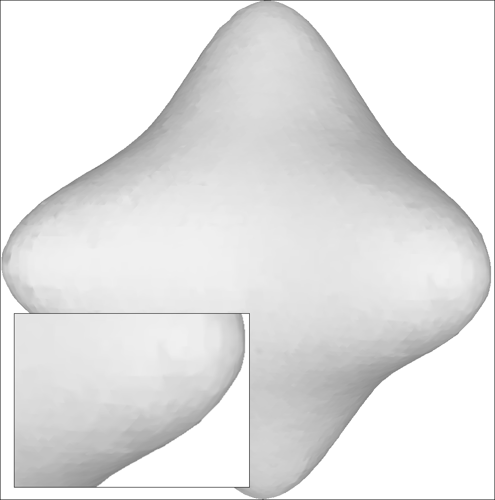
Ours

PU-GAN

ARGCN

Figure 10: Results of the mesh reconstruction from 4x upsampled point cloud with Poisson surface reconstruction.

TABLE X: Results of point cloud classification with PointNet [30] on the ModelNet40 testing set. After upsampling with Meta-PU, classification performance improved significantly.

#Points	512	2048	2048(from 512)
accuracy(%)	84.85	88.61	88.09

Mesh Reconstruction. Fig. 9 shows the visualized results of 3D surface reconstruction. In the 3D mesh reconstruction task, the result is greatly influenced by the density as well as the quality of the input point cloud. Unfortunately, the point cloud scanned from the real object is usually sparse and noisy due to the device limitations. As a result, arbitrary point cloud upsampling is the key to improving the mesh reconstruction quality, given the inputs with variable density. In Fig. 9, all results are reconstructed with the ball pivoting algorithm [31]. The quality of the mesh reconstructed by our model is much higher than the input and other methods. Also, our results fit the underlying surface of the object more smoothly.

In Fig. 10, we also compare the results of different upsampling methods with the Poisson surface reconstruction. Although the benefits of our method can be observed from the upsampled point cloud (upper row), the Poisson reconstruction results (lower row) show no significant advantage of any method. This is expected because with a stronger surface reconstruction method like Poisson, the noise level shown here can be handled.

Point Cloud Classification. In this application, we aim to demonstrate that point upsampling can potentially improve the classification results for sparse point clouds. In detail, we first train the PointNet on the ModelNet40 training set with $2048$ input points for each model. During testing, we prepare three datasets for each model: 1) $2048$ points uniformly sampled from the corresponding shape surface (referred to as “2048”); 2) $512$ points non-uniformly sampled from the $2048$ points (referred to as “512”); 3) the $4\times$ upsampling results obtained from the $512$ points with Meta-PU (referred as “2048(from 512)”). As shown in Table. X, because “512” is sparser than “2048”, it results in lower classification accuracy. By using Meta-PU for upsampling, “2048(from 512)” can achieve a significant performance gain and is comparable with the original “2048”.

Upsampling on an Unseen Dataset: SHREC15. We test Meta-PU on the unseen dataset SHREC15 [32] without fine-tuning, to further validate the generalizability of our model. The quantitative results are shown in Table IX.

Upsampling on an Unseen Dataset: Real-scanned LiDAR Points. Although Meta-PU is only trained on the Visionair dataset following the protocol in [4], it can generalize very well to the unseen real-scanned LiDAR point clouds from the KITTI dataset. We present some visual examples in Fig. 11, where the input point clouds are very sparse and non-uniform.

Figure 11: Upsampling results of Meta-PU on unseen LiDAR point clouds from the KITTI [33] dataset. The first row is the sparse real-data object-level input, and the second row is the corresponding output. The third row is the sparse real-data scene-level input, and the last row is its corresponding output. Meta-PU can generalize very well to unseen sparse and non-uniform LiDAR data.

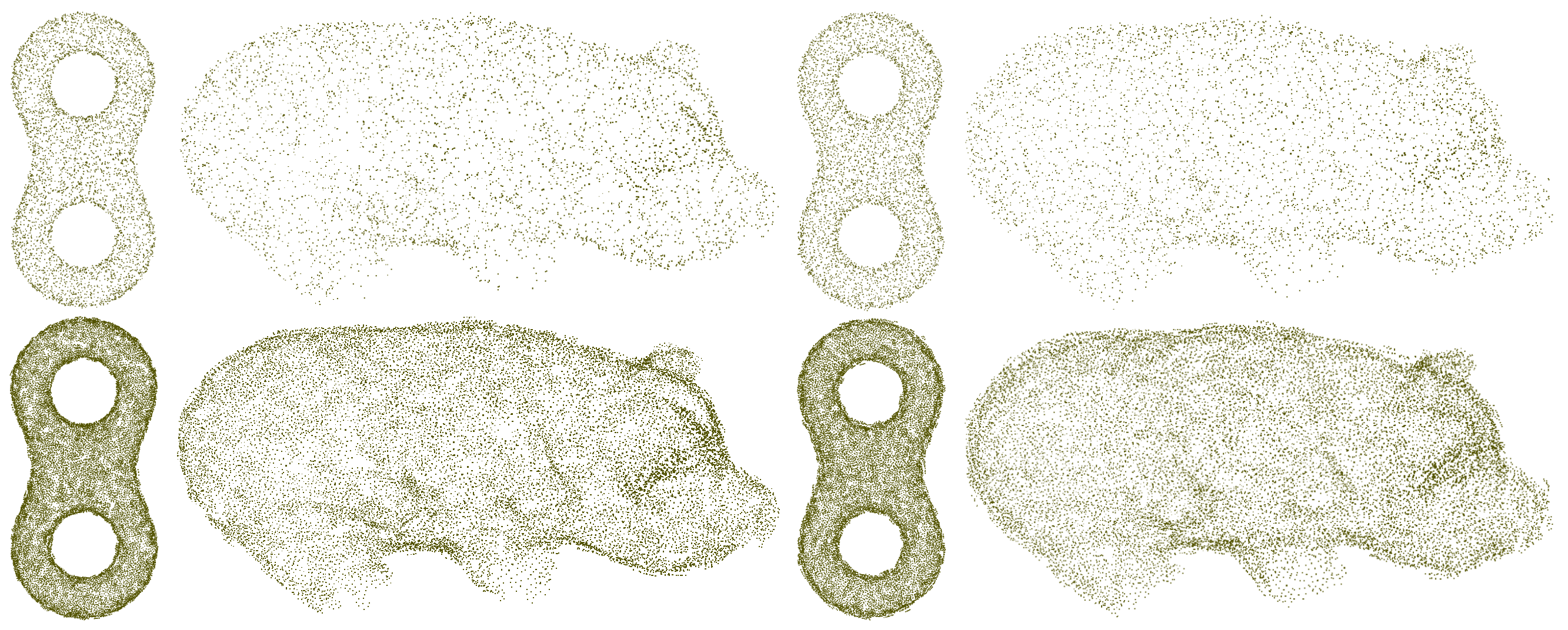
Figure 12: Results of up-sampling from noisy point clouds. The noise level $\sigma$ of the left two columns is $0.5\%$, and the right two is $1\%$. The scale factor is set to 4.

Upsampling With a Noisy Point Cloud. As depicted in Fig. 12, we use Meta-PU to upsample sparse point clouds jittered by Gaussian noise with various $\sigma$. With noisy and blurry inputs from the first row, our method can still stably generate smooth and uniformly distributed output.

Upsampling on Varying Input Sizes. Fig. 13 shows the upsampling results from input with different numbers of points with the scale $R=4$. It can be seen that Meta-PU is very robust to input points of various sizes and sparsities, even for the input with only $512$ points.

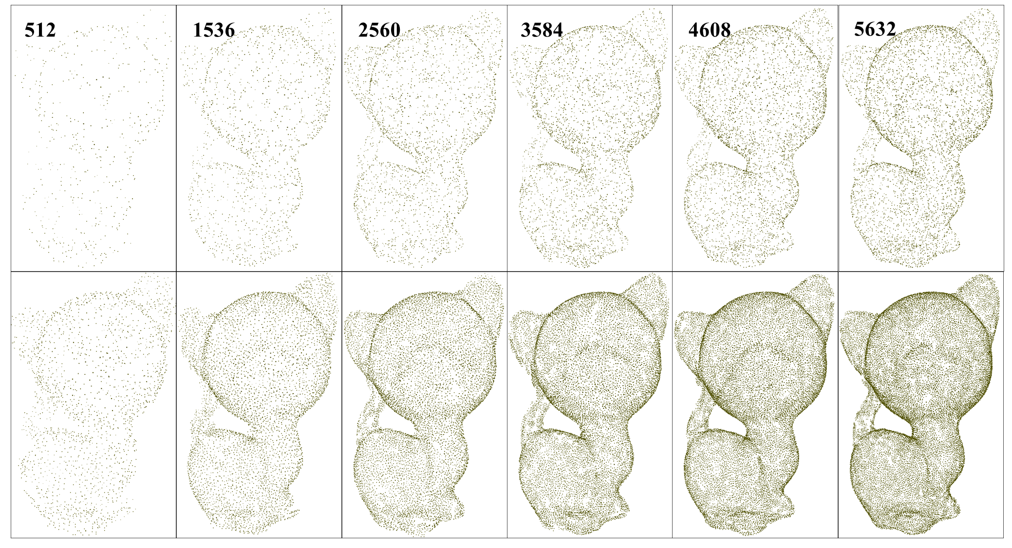
Figure 13: Upsampling results of Meta-PU from varying input sizes with the same scale of $4$. Our model is robust to various sizes and sparsities.

Upsampling on Non-integer Scales. Fig. 14 presents the results of upsampling the same sparse point cloud input for non-integer scales. Note that, though we did not train Meta-PU with such scales as $1.25,1.75,2.25,...$ explicitly, Meta-PU is still stable for these unseen scales, which is not supported by the existing point cloud upsampling baselines.

Figure 14: Comparison of point clouds upsampled for non-integer unseen scales from the same input with $5000$ points. Meta-PU is still stable on these unseen scales.

5 Conclusion

In this paper, we present Meta-PU, the first point cloud upsampling network that supports arbitrary scale factors (including non-integer factors). This method provides a more efficient and practical tool for 3D reconstruction, than the existing single-scale upsampling networks. The core part of Meta-PU is a novel meta-RGC block, whose weights are dynamically predicted by a meta-subnetwork, thus it can extract features tailored to the upsampling of different scales. The comprehensive experiments reveal that the joint training of multiple scale factors with one model improves performance. Our arbitrary-scale model even achieves better results at each specific scale than those single-scale state-of-the-art. The application on mesh reconstruction also demonstrates the superiority of our method in visual quality. Notably, similar to other upsampling methods, our method does not aim to fill holes, such that some large holes or missing parts still exist in the upsampled results. Another limitation is that the maximum upscale factor supported by our network is not infinity, constrained by the model size and GPU memory. These are all future directions worth exploring.

References

- [1] M. Alexa, J. Behr, D. Cohen-Or, S. Fleishman, D. Levin, and C. T. Silva, “Computing and rendering point set surfaces,” IEEE Transactions on Visualization and Computer Graphics, vol. 9, no. 1, pp. 3–15, Jan 2003.
- [2] H. Huang, D. Li, H. Zhang, U. Ascher, and D. Cohen-Or, “Consolidation of unorganized point clouds for surface reconstruction,” ACM Transactions on Graphics (Proc. SIGGRAPH Asia 2009), vol. 28, pp. 176:1–176:7, 2009.
- [3] S. Wu, H. Huang, M. Gong, M. Zwicker, and D. Cohen-Or, “Deep points consolidation,” ACM Trans. Graph., vol. 34, no. 6, pp. 176:1–176:13, Oct. 2015. [Online]. Available: http://doi.acm.org/10.1145/2816795.2818073
- [4] L. Yu, X. Li, C.-W. Fu, D. Cohen-Or, and P.-A. Heng, “Pu-net: Point cloud upsampling network,” in Proceedings of IEEE Conference on Computer Vision and Pattern Recognition (CVPR), 2018.
- [5] W. Yifan, S. Wu, H. Huang, D. Cohen-Or, and O. Sorkine-Hornung, “Patch-based progressive 3d point set upsampling,” in The IEEE Conference on Computer Vision and Pattern Recognition (CVPR), June 2019.
- [6] R. Li, X. Li, C.-W. Fu, D. Cohen-Or, and P.-A. Heng, “Pu-gan: A point cloud upsampling adversarial network,” in The IEEE International Conference on Computer Vision (ICCV), October 2019.
- [7] H. Wu, J. Zhang, and K. Huang, “Point cloud super resolution with adversarial residual graph networks,” 2019.
- [8] Q. Fan, D. Chen, L. Yuan, G. Hua, N. Yu, and B. Chen, “Decouple learning for parameterized image operators,” in Proceedings of the European Conference on Computer Vision (ECCV), 2018, pp. 442–458.
- [9] ——, “A general decoupled learning framework for parameterized image operators,” IEEE Transactions on Pattern Analysis and Machine Intelligence, 2019.
- [10] X. Hu, H. Mu, X. Zhang, Z. Wang, T. Tan, and J. Sun, “Meta-sr: A magnification-arbitrary network for super-resolution,” in Proceedings of the IEEE Conference on Computer Vision and Pattern Recognition, 2019, pp. 1575–1584.
- [11] Y. Lipman, D. Cohen-Or, D. Levin, and H. Tal-Ezer, “Parameterization-free projection for geometry reconstruction,” in ACM Transactions on Graphics (TOG), vol. 26, no. 3. ACM, 2007, p. 22.
- [12] C. R. Qi, H. Su, K. Mo, and L. J. Guibas, “Pointnet: Deep learning on point sets for 3d classification and segmentation,” in The IEEE Conference on Computer Vision and Pattern Recognition (CVPR), July 2017.
- [13] C. R. Qi, L. Yi, H. Su, and L. J. Guibas, “Pointnet++: Deep hierarchical feature learning on point sets in a metric space,” in Advances in Neural Information Processing Systems 30, I. Guyon, U. V. Luxburg, S. Bengio, H. Wallach, R. Fergus, S. Vishwanathan, and R. Garnett, Eds. Curran Associates, Inc., 2017, pp. 5099–5108. [Online]. Available: http://papers.nips.cc/paper/7095-pointnet-deep-hierarchical-feature-learning-on-point-sets-in-a-metric-space.pdf
- [14] Z. Chen, W. Zeng, Z. Yang, L. Yu, C. Fu, and H. Qu, “Lassonet: Deep lasso-selection of 3d point clouds,” IEEE Transactions on Visualization & Computer Graphics, vol. 26, no. 01, pp. 195–204, jan 2020.
- [15] Z. Shu, S. Xin, X. Xu, L. Liu, and L. Kavan, “Detecting 3d points of interest using multiple features and stacked auto-encoder,” IEEE Transactions on Visualization & Computer Graphics, vol. 25, no. 08, pp. 2583–2596, aug 2019.
- [16] H. Chen, M. Wei, Y. Sun, X. Xie, and J. Wang, “Multi-patch collaborative point cloud denoising via low-rank recovery with graph constraint,” IEEE Transactions on Visualization and Computer Graphics, pp. 1–1, 2019.
- [17] L. Yu, X. Li, C.-W. Fu, D. Cohen-Or, and P.-A. Heng, “Ec-net: an edge-aware point set consolidation network,” in The European Conference on Computer Vision (ECCV), September 2018.
- [18] I. Goodfellow, J. Pouget-Abadie, M. Mirza, B. Xu, D. Warde-Farley, S. Ozair, A. Courville, and Y. Bengio, “Generative adversarial nets,” in Advances in Neural Information Processing Systems 27, Z. Ghahramani, M. Welling, C. Cortes, N. D. Lawrence, and K. Q. Weinberger, Eds. Curran Associates, Inc., 2014, pp. 2672–2680. [Online]. Available: http://papers.nips.cc/paper/5423-generative-adversarial-nets.pdf
- [19] T. N. Kipf and M. Welling, “Semi-supervised classification with graph convolutional networks,” in International Conference on Learning Representations (ICLR), 2017.
- [20] M. Andrychowicz, M. Denil, S. Gomez, M. W. Hoffman, D. Pfau, T. Schaul, B. Shillingford, and N. De Freitas, “Learning to learn by gradient descent by gradient descent,” in Advances in neural information processing systems, 2016, pp. 3981–3989.
- [21] S. Ravi and H. Larochelle, “Optimization as a model for few-shot learning,” in International Conference on Learning Representations (ICLR), 2017.
- [22] T. Yang, X. Zhang, Z. Li, W. Zhang, and J. Sun, “Metaanchor: Learning to detect objects with customized anchors,” in Advances in Neural Information Processing Systems, 2018, pp. 320–330.
- [23] R. Hu, P. Dollár, K. He, T. Darrell, and R. Girshick, “Learning to segment every thing,” in Proceedings of the IEEE Conference on Computer Vision and Pattern Recognition, 2018, pp. 4233–4241.
- [24] D. Chen, Q. Fan, J. Liao, A. Aviles-Rivero, L. Yuan, N. Yu, and G. Hua, “Controllable image processing via adaptive filterbank pyramid,” IEEE Transactions on Image Processing, vol. 29, pp. 8043–8054, 2020.
- [25] Z. Liu, H. Mu, X. Zhang, Z. Guo, X. Yang, T. K.-T. Cheng, and J. Sun, “Metapruning: Meta learning for automatic neural network channel pruning,” arXiv preprint arXiv:1903.10258, 2019.
- [26] C. Lemke, M. Budka, and B. Gabrys, “Metalearning: a survey of trends and technologies,” Artificial intelligence review, vol. 44, no. 1, pp. 117–130, 2015.
- [27] S. M. Arnold, P. Mahajan, D. Datta, and I. Bunner, “learn2learn,” Sep. 2019. [Online]. Available: https://github.com/learnables/learn2learn
- [28] J. Feydy, T. Séjourné, F.-X. Vialard, S.-i. Amari, A. Trouvé, and G. Peyré, “Interpolating between optimal transport and mmd using sinkhorn divergences,” in The 22nd International Conference on Artificial Intelligence and Statistics. PMLR, 2019, pp. 2681–2690.
- [29] H. Huang, S. Wu, M. Gong, D. Cohen-Or, U. Ascher, and H. Zhang, “Edge-aware point set resampling,” ACM transactions on graphics (TOG), vol. 32, no. 1, pp. 1–12, 2013.
- [30] C. R. Qi, H. Su, K. Mo, and L. J. Guibas, “Pointnet: Deep learning on point sets for 3d classification and segmentation,” arXiv preprint arXiv:1612.00593, 2016.
- [31] F. Bernardini, J. Mittleman, H. E. Rushmeier, C. T. Silva, and G. Taubin, “The ball-pivoting algorithm for surface reconstruction,” IEEE Transactions on Visualization and Computer Graphics, vol. 5, pp. 349–359, 1999.
- [32] D. Pickup, X. Sun, P. L. Rosin, R. R. Martin, Z. Cheng, Z. Lian, M. Aono, A. Ben Hamza, A. Bronstein, M. Bronstein, S. Bu, U. Castellani, S. Cheng, V. Garro, A. Giachetti, A. Godil, J. Han, H. Johan, L. Lai, B. Li, C. Li, H. Li, R. Litman, X. Liu, Z. Liu, Y. Lu, A. Tatsuma, and J. Ye, “SHREC’14 track: Shape retrieval of non-rigid 3d human models,” in Proceedings of the 7th Eurographics workshop on 3D Object Retrieval, ser. EG 3DOR’14. Eurographics Association, 2014.
- [33] A. Geiger, P. Lenz, and R. Urtasun, “Are we ready for autonomous driving? the kitti vision benchmark suite,” in Conference on Computer Vision and Pattern Recognition (CVPR), 2012.