The scaling of social interactions across animal species
Abstract
Social animals self-organise to create groups to increase protection against predators and productivity. One-to-one interactions are the building blocks of these emergent social structures and may correspond to friendship, grooming, communication, among other social relations. These structures should be robust to failures and provide efficient communication to compensate the costs of forming and maintaining the social contacts but the specific purpose of each social interaction regulates the evolution of the respective social networks. We collate 611 animal social networks and show that the number of social contacts scales with group size as a super-linear power-law for various species of animals, including humans, other mammals and non-mammals. We identify that the power-law exponent varies according to the social function of the interactions as , with . By fitting a multi-layer model to our data, we observe that the cost to cross social groups also varies according to social function. Relatively low costs are observed for physical contact, grooming and group membership which lead to small groups with high and constant social clustering. Offline friendship has similar patterns while online friendship shows weak social structures. The intermediate case of spatial proximity ( and clustering dependency on network size quantitatively similar to friendship) suggests that proximity interactions may be as relevant for the spread of infectious diseases as for social processes like friendship.
Introduction
Social animals including humans live in groups to optimise the multiplicative benefits of social interactions such as protection, coordination, cooperation, access to information, and fitness, while balancing the competition, disease risk, and stress costs of group living [1, 2, 3]. Social interactions are fundamentally dyadic yet sufficiently diverse to link multiple animals or humans in connected social structures [1, 4, 5]. The purpose of social interactions is also diverse and spans a range of processes including communication, trust, grooming, dominance, or simply the loosely defined idea of friendship [1, 4, 6]. Correlations between social interactions, as for example dominance and physical contact, friendship ties maintained through communication, or the intertwined relation between trust and spatial proximity, reveal the complexity of social phenomena and suggest that common principles may underlie the formation of social ties.
A fundamental question concerns how the number of social connections depends on group size, and whether there are any emerging patterns in this relationship. The answer may reveal whether interaction patterns become more complex with size in order to maintain efficient social structures within the group. The cost to establish and maintain social contacts in small groups is relatively low but increases in larger groups [7]. This increasing costs leads to peer selection, either by necessity or affinity, up to a species-specific cognitive saturation point in the number of contacts one can manage [8]. Assuming that all members of a social group are reachable via social ties, in the limiting scenarios, a group of size individuals may have a fragile star-like structure with social ties to minimise social interactions (lowest cost) or a fully connected clique with ties (highest cost).
Evolutionary arguments support that social groups specialise and optimise social interactions to save resources while keeping or increasing the group efficiency [9, 10, 11], as for example in response to predators (ecological conditions) [12] or to fitness [13, 14]. There is also the argument that human social networks have an optimal size to optimise information transfer within groups [15]. Research on urban systems shows that human societies also organise in groups (e.g. cities) to optimise resources like infra-structure and to increase intellectual, social and economic outputs [16, 17]. These observations lead us to hypothesise that across species and social contexts, the number of social contacts scales with group size as , where and are positive constants.
Until recently, measuring social interactions was laborious. Past research relied on observations of animal and human behaviour or self-reporting of social contacts through questionnaires [4]. A natural limitation of these techniques is the size of the observed populations and potential recalling errors, as for example the inability to accurately identify or quantify each interaction [1, 4]. Electronic devices (e.g. mobile phones [18] or proximity sensors [19, 20]) and online platforms now provide means for passive and accurate recording of spatio-temporal location, communication between animals and between humans, among other forms of animal or human interactions. State-of-the-art electronic data collection is scalable but its ability to detect authentic social interactions may be questioned and should be treated cautiously [21, 22].
We collate extensive data to show empirically that the number of social contacts scales super-linearly (i.e. ) with group size and that social interactions can be categorised in different exponents independently of the animal species. We provide evidence that this scaling is necessary to maintain fundamental complex network structures irrespective of existing group sizes. We also fit our data to a social network model and show that a multi-layer structure and the cost of crossing social layers may explain the estimated scaling exponents.
| Social interaction type | Mammalian non-primates | Mammalian primates | Mammalian Humans | Actinopterygii | Aves | Insecta | Reptilia | Total |
|---|---|---|---|---|---|---|---|---|
| A: physical contact | 0 | 4 | 0 | 0 | 2 | 244 | 0 | 250 |
| B: grooming | 0 | 23 | 0 | 0 | 0 | 0 | 0 | 23 |
| C: group membership | 4 | 0 | 0 | 7 | 5 | 0 | 0 | 16 |
| D: spatial proximity | 63 | 58 | 88 | 9 | 0 | 12 | 1 | 231 |
| E: offline friendship | 0 | 0 | 67 | 0 | 0 | 0 | 0 | 67 |
| F: online friendship | 0 | 0 | 24 | 0 | 0 | 0 | 0 | 24 |
| Total | 67 | 85 | 179 | 16 | 7 | 256 | 1 | 611 |
Results
The data sets were collated using online databases of animal and human social networks previously analysed by other authors. All networks were reviewed for consistency and the data sets were standardised such that only unique pairs of social contacts were counted, i.e. self-loops, weighting, timings of contacts, and directions were removed. Social interactions were identified and labelled in the original studies by domain experts via direct observation (animal interactions), questionnaires (offline friendship), electronic devices (spatial proximity), and online platforms (online friendship) (see SI). To minimise potential ambiguities, each network was constructed based on the specific definition of social interaction in the respective original study. Table 1 shows the number of networks for each type of social interaction and animal class, including captive and free-ranging animals. The network size varies across species and social interactions because of experimental settings, characteristics and limitations of the study populations, e.g. the observation capacity of researchers, cost of technical devices, free-range vs. confined animals, online platforms, or animals living in small groups (see SI).
Scaling of social interactions
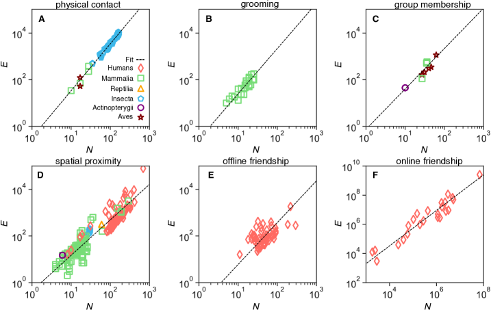
The networks of social interactions were grouped in categories following the type of social interactions as reported in the original studies (Table 1). Figure 1 shows the scaling between the number of social contacts and size (i.e. the number of interacting individuals) for each of the 6 original categories. We assume that the scaling of social relations is independent of species and test our hypothesis by fitting a power-law to the data using logarithmic transformed variables to evenly distribute the data points:
| (1) |
The fitting exercise gives super-linear power-law exponents (i.e. ) and strong linear correlations () for all categories of social interactions (Table 2). Assuming a small error in , the exponents follow the general law () with for online friendship (), for spatial proximity (), for group membership () and offline friendship (), and for physical contacts () and grooming (), despite differences in species and sample sizes (Fig. 1).
| Social interaction type | Pearson | -value | |||||
|---|---|---|---|---|---|---|---|
| best fit | CI | best fit | CI | correlation | |||
| A: physical contact | 250 | 2.01 | [1.98,2.04] | 0.75 | [0.33,1.68] | 0.96 | <.01 |
| B: grooming | 23 | 1.94 | [1.53,2.36] | 0.28 | [0.09,0.86] | 0.82 | <.01 |
| C: group membership | 16 | 1.73 | [1.47,1.99] | 0.33 | [0.29,0.37] | 0.89 | <.01 |
| D: spatial proximity | 231 | 1.52 | [1.45,1.59] | 0.44 | [0.34,0.58] | 0.55 | <.01 |
| E: offline friendship | 67 | 1.79 | [1.30,2.29] | 0.10 | [0.01,0.65] | 0.57 | <.01 |
| F: online friendship | 24 | 1.22 | [1.06,1.37] | 0.44 | [0.06,3.36] | 0.99 | <.01 |
This super-linear scaling indicates increasing densification of social contacts, that is, larger social groups have on average more social contacts per-capita than the smaller ones. It is not surprising that because the number of social connections must scale at least linearly with group size () to maintain the social network connected; this is known as the percolation threshold in random networks [23]. If , small perturbations may fragment the network, breaking down the group structure. Furthermore, suggests that a super-linear number of contacts are necessary to create and maintain the complex social network structures for the groups to function cost-efficiently irrespective of size.
Social network structure
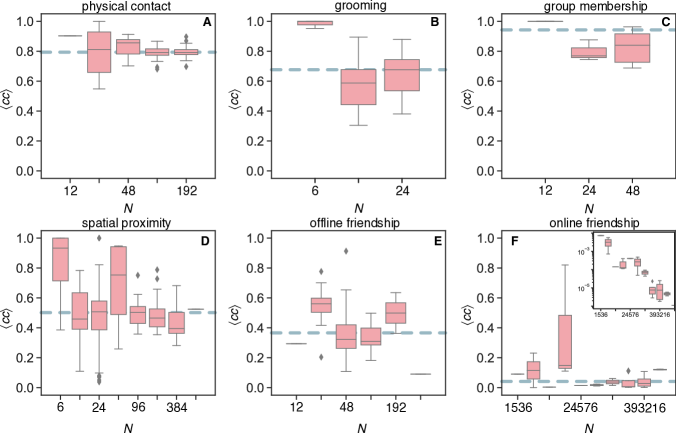
We study the network structures for each of the six types of social interactions (See Methods). The clustering coefficient is a local measure of the level of sociality between common contacts of a focal individual (i.e. the fraction of social triangles). Its intensity indicates an evolutionary group advantage as for example fitness benefits [24, 25]. Networks with higher clustering are relatively more robust since the deletion of a social connection would not significantly affect interaction and communication among close contacts. In our social networks, is constant for varying network size for all types of social contacts (Fig. 2). In random networks, the clustering coefficient decays with increasing network size as , where is the average number of contacts (or edges) in the network [23]. The inset of Fig. 2F shows the results for the randomised versions of the same online friendship networks (see SI for the other categories). In all categories, there is a higher clustering coefficient than expected on the basis of randomised social contacts (See caption Fig. 2). Since the average degree is defined as , we have and thus would need to have constant clustering in random networks. Evolutionary theory implies that more complex structures may emerge in such social systems to optimise resources, e.g. to reap the fitness related benefits, and thus relatively less social contacts become necessary to reach the same level of clustering across group sizes [24, 25]. For example, for some classes of random heterogeneous networks, , where the proportionality constant depends on the heterogeneity of the distribution of contacts among individuals and is lower than [23].
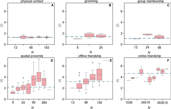
The average length of the shortest-paths measures the average distance between any pairs of individuals in the social network and quantifies the communication potential between parts of the network [26]. Shorter average distances (i.e. , resulting in the small-world effect [27]) indicate that information flows quickly over the network, which is a fundamental characteristic of efficient group organisation [28]. For physical contacts, grooming, and group membership, is constant and slightly higher than one (Fig. 2A-C). For spatial proximity and offline friendship, the values increase with size following quantitatively similar trends (Fig. 2D-E). The results for online friendship suggest a constant trend (Fig. 2F). In all cases, the average path-length is , which is the small-world horizon observed empirically [23]. For all 6 categories, the random versions of the same networks give constant relations albeit generally with lower values (see SI). In theoretical random networks, the average distance increases slowly with the network size as [23]. Nevertheless, the average path-length is approximately constant across group sizes if for , since in this case . Smaller thus leads to higher , as observed in the analysed networks. In some classes of heterogeneous random networks, is also nearly constant with network size [23]. The density of contacts explains the low for physical contact, grooming and group membership. The discrepancy of spatial proximity, offline and online friendship with the random case indicates that more complex network structures are being formed in larger groups for these types of social interactions. In sparse networks, like those, a high level of local clustering increases the distance between random pairs of network nodes because of local spots of connectivity redundancy [23]. Taken together, the constant clustering across network sizes (Fig. 2) implies that the average distance will necessarily increase (Fig. 3), unless followed by a sufficient increase in the number of connections (to maintain low average distances as the group increases). The growth in offline friendship followed by a seemingly constant pattern for online friendship (which has larger sizes) suggests a potential saturation in for human friendship in line with the small-world horizon observed in previous studies [23]. Although communication remains efficient (because ), the benefits of forming larger groups do not compensate the costs of optimising certain network structures, as is the case for other types of social interactions involving physical contact.
Multi-layer model
Multi-layer models can be used to represent the underlying generative mechanisms through which individuals combine skills and affinity to build up more complex social groups. From single individuals to the entire population, individuals may be stratified in layers (or levels) corresponding to different groups [29]. For example, living in households (layer 1) within neighbourhoods (layer 2) that in turn are part of cities (layer 3), and so on, seems natural for humans. While people mostly interact with those in the same group (e.g. within the same household), interactions across groups are less frequent [30] (e.g. between different households in the same neighbourhood). Interactions across groups at the same layer are necessary to define higher-order groups, i.e. a group at the next higher layer, as for example a neighbourhood is a result of interactions between individuals from different households. Multi-layer models have been used to explain spatial relations in vascular [31] and infrastructure [17] systems. We argue that such models are also of value for social groups, not necessarily spatially bound, since multi-layer organisation has been observed across animal species in which a relation between group sizes in different layers vary from nearly 2.5 in primates to about 3 for other mammals including humans [32, 14]. This means that individuals are organised as multiples of 3, for example, in groups of 5 (layer 1), 15 (layer 2), 45 (layer 3), and so on. The model detailed below does not aim to reproduce all structures of the 611 analysed networks but focuses on the scaling exponents .
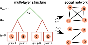
The self-similar multi-layer group structure is mathematically represented as a branching tree with a group at layer split into sub-groups at layer (Fig. 4). At the highest layer , all individuals belong to a single social group, i.e. , and at the lowest layer (), each group is formed by a single unique individual. In this model, individuals and make a social contact with probability dependent on the distance between the layers that separate them. Closer individuals (e.g. at distance because they are living in the same neighbourhood or belonging to the same social group) are more likely to interact than individuals living far apart (e.g. at distance because they are living in different cities or belonging to different social groups), i.e. decreases with . The multi-layer tree-like structure only defines the distance between the groups that is in turn used to form contacts in the social network (Fig. 4); the resulting social network only has tree-like structure for sparse networks, i.e. when . The self-similarity between layers implies that [33]. A power-law of the form , with , satisfies this relationship. The parameter represents the cost to make social interactions across layers, that we assume is lower than the cost to create a new layer, i.e. , because multiple contacts are necessary to establish a new layer. For a given individual , the expected number of social connections is:
For , the sum converges:
Since and , we get:
Therefore, the total number of social connections is:
The multi-layer model implies that . Assuming that [14], the cost of connections is thus for physical contact (), for grooming (), for group membership (), for spatial proximity (), for offline friendship () and for online friendship (). This cost is associated to crossing (virtual) barriers between social groups that might cause the creation of larger groups. The low cost () for physical contact and grooming means that , i.e. the probability to form connections is independent of the social distance , collapsing the assumption of multi-layer structure. For such types of social interactions, the connections within the same social group are favoured; individuals do not groom in different social groups nor make persistent physical contacts, except physical contacts for conflict that would not be reflected in our data. This effect is related to the high clustering coefficient reported in previous sections and may explain the relatively small size of such networks. The number of social contacts for such activities is limited within the same social group.
Online friendship, on the other hand, is costly () in terms of crossing social boundaries to connect individuals from different social groups [34], e.g. with different tastes, ideas, location, age, and so on. Socially closer individuals would be favoured here as well since it is harder to be friends with dissimilar people than with those similar to each other [30]. However, given that online connections are cheap to establish and maintain (i.e. do not need nurturing and resources), the multi-layer structure becomes relevant with a non-negligible number of socially distant connections being formed. Furthermore, online friendship typically mixes (real) friends, acquaintances, relatives, and co-workers, each belonging to different social groups, with some individuals acting as social brokers. For example, online friendship is more easily established between those studying in the same school than at different schools; however, inter-school friendship is facilitated by the online platform, though socially costly (lack of face-to-face interactions, no common friends, building trust). For networks derived from mobile phone communication in urban populations, a scaling exponent has been reported [35, 36, 37]. Such mobile communication data sets mix professional and personal relations which possibly also leads to higher costs in the sense of crossing social boundaries. In one study, a constant clustering coefficient has been also observed suggesting that similar underlying principles may explain the formation of such social or communication structures [37]. The multi-layer structure becomes less relevant for offline friendship () that are typically more spatially constrained in our data. For example, students or prison inmates will report friendship with those around them. In schools, from where most of our data come from, the social structure is seen at the class and school layers only. Given experimental limitations, it is often not possible to report friends outside the study setting, which could reveal higher social layers, e.g. neighbourhood friends. It is possible that the exponent for friendship is thus between what we estimated for offline and online friendship if all layers of friends and not only those in the same study setting were reported.
Our analysis finds an intermediate exponent () and cost () for spatial proximity. Spatial proximity is a particular type of social interaction. Grooming, physical contact and human friendship are well-defined interactions identified, respectively, by observing joint activities or by directly inquiring individuals. However, spatial proximity interactions are measured by sensors or direct observation and capture a mixture of social situations. Spatial proximity might reflect affinity, trust and friendship between individuals and animals sharing the same space [30], e.g. persistent spatial proximity between pairs of cows [38], or behavioural or trait similarity, i.e. homophily, as for example friends visiting a museum [39] or health-care workers in hospitals [40]. On the other hand, spatial proximity interactions might simply reflect spatial constrains forcing individuals and animals to be in close proximity during periods of time, e.g. a group of visitors of an art exhibition [39] or confined animals [38]. Nevertheless, also in the later, affinity and trust are reflected in the proximity contacts. As discussed above, it is possible that friendship at the society layer likely follows patterns intermediate to those observed in the online () and offline () categories. The existing literature associating friendship to time that individuals spent together [30] and the observation that spatial proximity contacts follow an intermediate exponent () suggest a potential link between these social interactions. We cannot make a strong association between the two types of social interactions due to lack of data of offline friendship in larger populations. Previous modelling exercises in urban populations suggest that can be explained by mobility (, where is the Hausdorff dimension of a path in space) over two dimensional () spaces based on the assumption that fully-mixed populations may fully explore a given area [17]. While this assumption may hold within, e.g. schools, museums or barns, it does not apply on larger spatial areas since humans and animals are territorial and tend to spend most of time within certain locations [41] or with certain individuals [30]. On the other hand, the same model suggests that contacts per-capita scale as (i.e. ) under the same conditions (i.e. ). This fits well to our findings for offline friendship, where people may virtually explore the whole social space and potentially interact with different individuals.
Conclusions
Our findings reveal key aspects of the organisation of animal social networks. Though primates and non-primates (including humans) are more represented than other animals in our data set, the universal scaling relations between the number of social contacts and size suggest common organisation principles across animal species that can be explained by multi-layer models designed to maintain the functioning of the social groups [32, 14]. Different scaling exponents following the general relation , with allow us to distinguish types of social interactions and to infer network structures underlying those interactions. For all types of social interactions, the local clustering remains constant for increasing network sizes albeit having different intensity in each case. Physical contacts, grooming and group membership have similar constant median values that are higher than observed for spatial proximity, offline and online friendships. The average path-length is also constant and follow the small-world pattern (i.e. ) for most cases with the exception of spatial proximity and offline friendship where a quantitatively similar positive trend is observed with values below the small-world horizon of previously observed in social networks [23].
One may argue that humans differ from other animals by developing more efficient social network structures, with relatively less contacts for higher network sizes, and thus lowering the scaling exponents. There is a quantifiable relationship with brain and group sizes, along with the complexity of the interactions. Humans are able to process the cognitive demand of other forms of relationships such as friendship, rather than mating and dominance relations that often occur within other animals and species [42]. The common scaling pattern observed across species and particularly for spatial proximity weakens the hypothesis that animals differ. Our results suggest that the type of social interaction, and to a lesser extent, the group size, are more relevant to determine the scaling exponents than the animal species. We reached this conclusion by combining data from different species. More statistical power could be achieved with a larger sample of network data for specific combinations of social interactions and species in order to study these relations separately. Given the multi-layer structure of social networks and experimental constraints, offline friendship data sets are limited to relatively small social circles [30]. If one could map higher social layers, the scaling exponent could decrease, likely to the same value as observed for spatial proximity. If this is confirmed in future studies, we will be able to infer that spatial proximity is a proxy of friendship across animals species [30].
Physical contact, grooming and group membership are associated with more robust and topologically efficient networks (since clustering is higher and path-lengths are shorter) than friendship and proximity interactions. This social cohesion is a result of homophily and coordination to maintain group functioning, which likely creates smaller groups in these categories relative to friendship and proximity categories because of the cost of nurturing contacts. The frequency and number of social interactions leading to stable social contacts are also important to regulate diffusion processes such as communication [26], innovation [16, 17], infectious diseases [19, 43] and social phenomena [30, 44]. Our results suggest that physical contacts and grooming are more efficient than proximity to facilitate spread phenomena at the population (network) level. Online friendships are associated to looser social structures easier to fragment as the groups increase in size. The relatively high cost of nurturing too many online social contacts across social layers restrains the opportunities to generate higher clustering or common friends, and create redundant structures, as observed in the smaller networks related to activities necessary to keep the group functioning.
Although we focus on temporally stable social networks [45], the availability of temporal information and intensity of certain social interactions could also help to understand the formation and dissolution of social contacts and how particular network structures are formed. Future research should add a quality measure to social interactions (e.g. via weights or temporal dynamics) to investigate the varying importance of creating and maintaining particular structures [46]. Strong super-linear scaling implies prohibitive social costs to maintain larger groups for some types of social interactions. The questions on whether there is a maximum or optimal group size in which efficient groups can exist and fitness is maximised [47], or whether more complex network structures are necessary to sustain larger groups, remains open.
Methods
Data
The data sets used in this study were collected using public network data repositories. A list of repositories and a full list of the original references for the 611 data sets are available in the SI. The 6 types of social interactions: physical contact, grooming, group membership, spatial proximity, offline friendship and online friendship were identified and labelled in the original studies by domain experts via direct observation (animal interactions), questionnaires (offline friendship), electronic devices (spatial proximity), and online platforms (online friendship). All 611 networks were standardised for the analysis, including the removal of self-loops, edge directions, and edge weights.
Networks
A network of size is defined as a set of nodes and a set of edges connecting nodes and . A node represents either a person or an animal. An edge represents a social connection of a specific type. In an undirected network, edges are reciprocal, i.e. . In a network without self-loops, there is no edge .
The clustering coefficient of a node is given by:
| (2) |
where is the number of edges between the nodes directly connected to node . The average clustering coefficient of the network is thus:
| (3) |
The topological distance between the nodes and is the length of the shortest-path in number of edges. It is calculated within the largest connected component of the network . In the largest connected component, there is at least one path between any pairs of nodes and . The average shortest-path length is:
| (4) |
References
- [1] Krause, J. & Ruxton, G. Living in Groups (Oxford University Press, 2002).
- [2] Molvar, E. & Bowyer, R. Costs and Benefits of Group Living in a Recently Social Ungulate: The Alaskan Moose. \JournalTitleJournal of Mammalogy 75, 621–630 (1994).
- [3] Seabright, P. The Company of Strangers: A Natural History of Economic Life (Princeton University Press, 2010).
- [4] Wasserman, S. & Faust, K. Social Network Analysis: Methods and Applications (Cambridge University Press, 1994).
- [5] Faust, K. & Skvoretz, J. Comparing Networks Across Space and Time, Size and Species. \JournalTitleSociological Methodology 32, 267–299 (2002).
- [6] Caroline, H. Explorations of close friendship: A concept analysis. \JournalTitleArchives of Psychiatric Nursing 7, 236–243 (1993).
- [7] Sueur, C., Deneubourg, J.-L., Petit, O. & Couzin, I. D. Group size, grooming and fission in primates: a modeling approach based on group structure. \JournalTitleJournal of Theoretical Biology 273, 156–166 (2011).
- [8] Dunbar, R. Neocortex size as a constraint on group size in primates. \JournalTitleJournal of Human Evolution 22, 469–493 (1992).
- [9] Terborgh, J. & Janson, C. The socioecology of primate groups. \JournalTitleAnnual Review of Ecology and Systematics 17, 111–136 (1986).
- [10] Guindre-Parker, S. & Rubenstein, D. Survival benefits of group living in a fluctuating environment. \JournalTitleThe American Naturalist 195, 1027–1036 (2020).
- [11] Pasquaretta, C. et al. Social networks in primates: smart and tolerant species have more efficient networks. \JournalTitleScientific reports 4, 1–8 (2014).
- [12] Williams, C., Lutz, R. & Applegate, R. Optimal group size and northern bobwhite coveys. \JournalTitleAnimal Behaviour 66, 377–387 (2003).
- [13] Roberts, A. & Roberts, S. Communicative roots of complex sociality and cognition. \JournalTitleBiological Reviews 95, 51–73 (2020).
- [14] Dunbar, R., Carron, P. M. & Shultz, S. Primate social group sizes exhibit a regular scaling pattern with natural attractors. \JournalTitleBiology Letters 14, 20170490 (2018).
- [15] West, B. et al. Relating size and functionality in human social networks through complexity. \JournalTitleProceedings of the National Academy of Sciences 117, 18355–18358 (2020).
- [16] Bettencourt, L., Lobo, J., Helbing, D., Kühnert, C. & West, G. Growth, innovation, scaling, and the pace of life in cities. \JournalTitleProceedings of the National Academy of Sciences USA 104, 7301–7306 (2007).
- [17] Bettencourt, L. The origins of scaling in cities. \JournalTitleScience 340, 1438–1441 (2013).
- [18] Eagle, N. & Pentland, A. Reality mining: sensing complex social systems. \JournalTitleJournal Personal and Ubiquitous Computing 10, 255–268 (2004).
- [19] Barrat, A., Cattuto, C., Tozzi, A., Vanhems, P. & Voirin, N. Measuring contact patterns with wearable sensors: methods, data characteristics and applications to data-driven simulations of infectious diseases. \JournalTitleClinical Microbiology Infections 20, 10–16 (2014).
- [20] Migliano, A. B. et al. Characterization of hunter-gatherer networks and implications for cumulative culture. \JournalTitleNature Human Behaviour 1, 1–6 (2017).
- [21] Kibanov, M. et al. Is web content a good proxy for real-life interaction? In Proceedings of the 2015 ACM/IEEE International Conference on Advances in Social Networks Analysis and Mining, ASONAM 2015, Paris, France, August 2015 (2015).
- [22] Lieberman, A. & Schroeder, J. Two social lives: How differences between online and offline interaction influence social outcomes. \JournalTitleCurrent Opinion Psychology 31, 16–21 (2020).
- [23] Newman, M. Networks: An Introduction (Oxford University Press, 2010).
- [24] Delius, J. & Siemann, M. Transitive responding in animals and humans: Exaptation rather than adaptation? \JournalTitleBehavioural Processes 42, 107–137 (1998).
- [25] Cheney, D., JB, Silk & Seyfarth, R. Network connections, dyadic bonds and fitness in wild female baboons. \JournalTitleRoyal Society Open Science 3, 160255 (2016).
- [26] Latora, V. & Marchiori, M. Efficient behavior of small-world networks. \JournalTitlePhysical Review Letters 87, 198701 (2001).
- [27] Travers, J. & Milgram, S. An experimental study of the small world problem. \JournalTitleSociometry 32, 425–443 (1969).
- [28] Schnettler, S. A structured overview of 50 years of small-world research. \JournalTitleSocial networks 31, 165–178 (2009).
- [29] Watts, D., Dodds, P. S. & Newman, M. Identity and search in social networks. \JournalTitleScience 296, 1302–1305 (2002).
- [30] Dunbar, R. Structure and function in human and primate social networks: implications for diffusion, network stability and health. \JournalTitleProceedings of the Royal Society A 476 (2020).
- [31] West, G., Brown, J. & Enquist, B. The fourth dimension of life: Fractal geometry and allometric scaling of organisms. \JournalTitleScience 284, 1677–1679 (1999).
- [32] Hill, R., Bentley, R. & Dunbar, R. Network scaling reveals consistent fractal pattern in hierarchical mammalian societies. \JournalTitleBiology Letters 4 (2008).
- [33] Leskovec, J., Kleinberg, J. & Faloutsos, C. Graphs over time: Densification laws, shrinking diameters and possible explanations. In KDD’05, August 21-24, 2015, Chicago, Illinois, USA (2005).
- [34] Tamarit, I., Cuesta, J., Dunbar, R. & Sanchez, A. Cognitive resource allocation determines the organization of personal networks. \JournalTitleProceedings of the National Academy of Sciences 115 (2018).
- [35] Calabrese, F. et al. The connected states of america: Quantifying social radii of influence. In 2011 IEEE Third International Conference on Privacy, Security, Risk and Trust and 2011 IEEE Third International Conference on Social Computing, 223–230 (2011).
- [36] Pan, W., Ghoshal, G., Krumme, C., Cebrian, M. & Pentland, A. Urban characteristics attributable to density-driven tie formation. \JournalTitleNature Communication 4 (2013).
- [37] Schläpfer, M. et al. The scaling of human interactions with city size. \JournalTitleJournal Royal Society Interface 11, 20130789 (2014).
- [38] Rocha, L., Terenius, O., Veissier, I., Meunier, B. & Nielsen, P. Persistence of sociality in group dynamics of dairy cattle. \JournalTitleApplied Animal Behaviour Science 223 (2020).
- [39] Isella, L. et al. What’s in a crowd? analysis of face-to-face behavioral networks. \JournalTitleJournal of Theoretical Biology 271, 166–180 (2011).
- [40] Vanhems, P. et al. Estimating potential infection transmission routes in hospital wards using wearable proximity sensors. \JournalTitlePLoS ONE 8, e73970 (2013).
- [41] Song, C., Qu, Z., Blumm, N. & Barabási, A.-L. Limits of predictability in human mobility. \JournalTitleScience 327, 1018–1021 (2010).
- [42] Dunbar, R. The social brain hypothesis and its implications for social evolution. \JournalTitleAnnals of Human Biology 36, 562–572 (2009).
- [43] Rocha, L., Thorson, A. & Lambiotte, R. The non-linear health consequences of living in larger cities. \JournalTitleJournal of Urban Health 92, 785–799 (2015).
- [44] Alves, L., Ribeiro, H., Lenzi, E. & Mendes, R. Distance to the scaling law: A useful approach for unveiling relationships between crime and urban metrics. \JournalTitlePLoS ONE 8 (2013).
- [45] Rocha, L., Masuda, N. & Holme, P. Sampling temporal networks: Methods and biases. \JournalTitlePhysical Review E 96 (2017).
- [46] Farine, D. & Whitehead, H. Constructing, conducting and interpreting animal social network analysis. \JournalTitleJournal of Animal Ecology 84, 1144–1163 (2015).
- [47] Ward, A. & Webster, M. The evolution of group living. In Ward, A. & Webster, M. (eds.) Sociality: The Behaviour of Group-Living Animals, 191–216 (Springer International Publishing, 2016).
Acknowledgements
The authors thank Luana de Freitas Nascimento for helpful discussions.
Author contributions statement
L.R. designed the research, made the analysis and wrote the draft; J.R., K.S., M.S. contributed with methods; All authors revised the manuscript.
Additional information
There are no competing interests.