Data-driven design of targeted gene panels for estimating immunotherapy biomarkers

Abstract

We introduce a novel data-driven framework for the design of targeted gene panels for estimating exome-wide biomarkers in cancer immunotherapy. Our first goal is to develop a generative model for the profile of mutation across the exome, which allows for gene- and variant type-dependent mutation rates. Based on this model, we then propose a new procedure for estimating biomarkers such as tmb and tib. Our approach allows the practitioner to select a targeted gene panel of a prespecified size, and then construct an estimator that only depends on the selected genes. Alternatively, the practitioner may apply our method to make predictions based on an existing gene panel, or to augment a gene panel to a given size. We demonstrate the excellent performance of our proposal using data from three nsclc studies, as well as data from six other cancer types. Keywords: cancer, gene panel design, targeted sequencing, tumour indel burden, tumour mutation burden.

1 Introduction

It has been understood for a long time that cancer, a disease occurring in many distinct tissues of the body and giving rise to a wide range of presentations, is initiated and driven by the accumulation of mutations in a subset of a person’s cells (boveri_concerning_2008). Since the discovery of Immune Checkpoint Blockade (ICB) (ishida_induced_1992, leach_enhancement_1996), there has been an explosion of interest in cancer therapies targeting immune response and ICB therapy is now widely used in clinical practice (robert_decade_2020). ICB therapy works by targeting natural mechanisms (or checkpoints) that disengage the immune system, for example the proteins Cytotoxic T Lymphocyte Associated protein 4 (CTLA-4) and Programmed Death Ligand 1 (PD-L1) (buchbinder_ctla-4_2016). Inhibition of these checkpoints can promote a more aggressive anti-tumour immune response (pardoll_blockade_2012), and in some patients this leads to long-term remission (borghaei_five-year_2021). However, ICB therapy is not always effective (nowicki_mechanisms_2018) and may have adverse side-effects, so determining which patients will benefit in advance of treatment is vital.

Exome-wide prognostic biomarkers for immunotherapy are now well-established – in particular, Tumour Mutation Burden (TMB) is used to predict response to immunotherapy (zhu_association_2019, cao_high_2019). TMB is defined as the total number of non-synonymous mutations occurring throughout the tumour exome, and can be thought of as a proxy for how easily a tumour cell can be recognised as foreign by immune cells (chan_development_2019). However, the cost of measuring TMB using Whole Exome Sequencing (WES) (sboner_real_2011) currently prohibits its widespread use as standard-of-care. Sequencing costs, both financial and in terms of the time taken for results to be returned, are especially problematic in situations where high-depth sequencing is required, such as when utilising blood-based circulating tumour DNA (ctDNA) from liquid biopsy samples (gandara_blood-based_2018). The same issues are encountered when measuring more recently proposed biomarkers such as Tumour Indel Burden (TIB) (wu_tumor_2019, turajlic_insertion-and-deletion-derived_2017), which counts the number of frameshift insertion and deletion mutations. There is, therefore, demand for cost-effective approaches to estimate these biomarkers (fancello_tumor_2019, golkaram_interplay_2020).

In this paper we propose a novel, data-driven method for biomarker estimation, based on a generative model of how mutations arise in the tumour exome. More precisely, we model mutation counts as independent Poisson variables, where the mean number of mutations depends on the gene of origin and variant type, as well as the Background Mutation Rate (BMR) of the tumour. Due to the ultrahigh-dimensional nature of sequencing data and the fact that in many genes mutations arise purely according to the BMR, we use a regularisation penalty when estimating the parameters of the model. In addition, this identifies a subset of genes that are mutated above or below the background rate. Our model facilitates the construction of a new estimator of TMB, based on a weighted linear combination of the number of mutations in each gene. The vector of weights is chosen to be sparse (i.e. have many entries equal to zero), so that our estimator of TMB may be calculated using only the mutation counts in a subset of genes. In particular, this allows for accurate estimation of TMB from a targeted gene panel, where the panel size (and therefore the cost) may be determined by the user.

We demonstrate the excellent practical performance of our framework using a Non-Small Cell Lung Cancer (NSCLC) dataset (campbell_distinct_2016), and include a comparison with existing state-of-the-art approaches for estimating TMB. We further validate these results by testing the performance on data from two more NSCLC studies (hellmann_genomic_2018, rizvi_mutational_2015). Moreover, since our model allows variant type-dependent mutation rates, it can be adapted easily to predict other biomarkers, such as TIB. Our method may also be used in combination with an existing targeted gene panel. In particular, we can estimate a biomarker directly from the panel, or first augment the panel and then construct an estimator. Finally, in order to further investigate the utility of our proposal across a range of mutation profiles, we use it to select targeted gene panels and estimate TMB in six other cancer types.

Due to its emergence as a biomarker for immunotherapy in recent years, a variety of groups have considered methods for estimating TMB. A simple and common way to estimate TMB is via the proportion of mutated codons in a targeted region. budczies_optimizing_2019 investigate how the accuracy of predictions made in this way are affected by the size of the targeted region, where mutations are assumed to occur at uniform rate throughout the genome. More recently yao_ectmb_2020 modelled mutations as following a negative binomial distribution while allowing for gene-dependent rates, which are inferred by comparing nonsynonymous and synonymous mutation counts. In contrast, our method does not require data including synonymous mutations. Where they are included, we do not assume that synonymous mutations occur at a uniform rate throughout the genome, giving us the flexibility to account for location-specific effects on synonymous mutation rate such as chromatin configuration (makova_effects_2015) and transcription-dependent repair mechanisms (fong_intertwined_2013). Linear regression models have been used for both panel selection (lyu_mutation_2018) and for biomarker prediction (guo_exon_2020). A review of some of the issues arising when dealing with targeted panel-based predictions of TMB biomarkers is given by wu_designing_2019. Finally, we are unaware of any methods for estimating TIB from targeted gene panels.

The remainder of the paper is as follows. In Section 2, we introduce our NSCLC data sources, and provide a detailed description of our methodological proposal. The full demonstration of our method using the NSCLC dataset is given in Section 3. Section LABEL:sec:robust provides several further analyses to investigate the robustness of our proposal in other cancer types and we conclude in Section LABEL:sec:conclusion. We also provide an R package ICBioMark (bradley_icbiomark_2021) which implements the methodology and reproduces the experimental results in the paper.

2 Methodology

2.1 Data and terminology

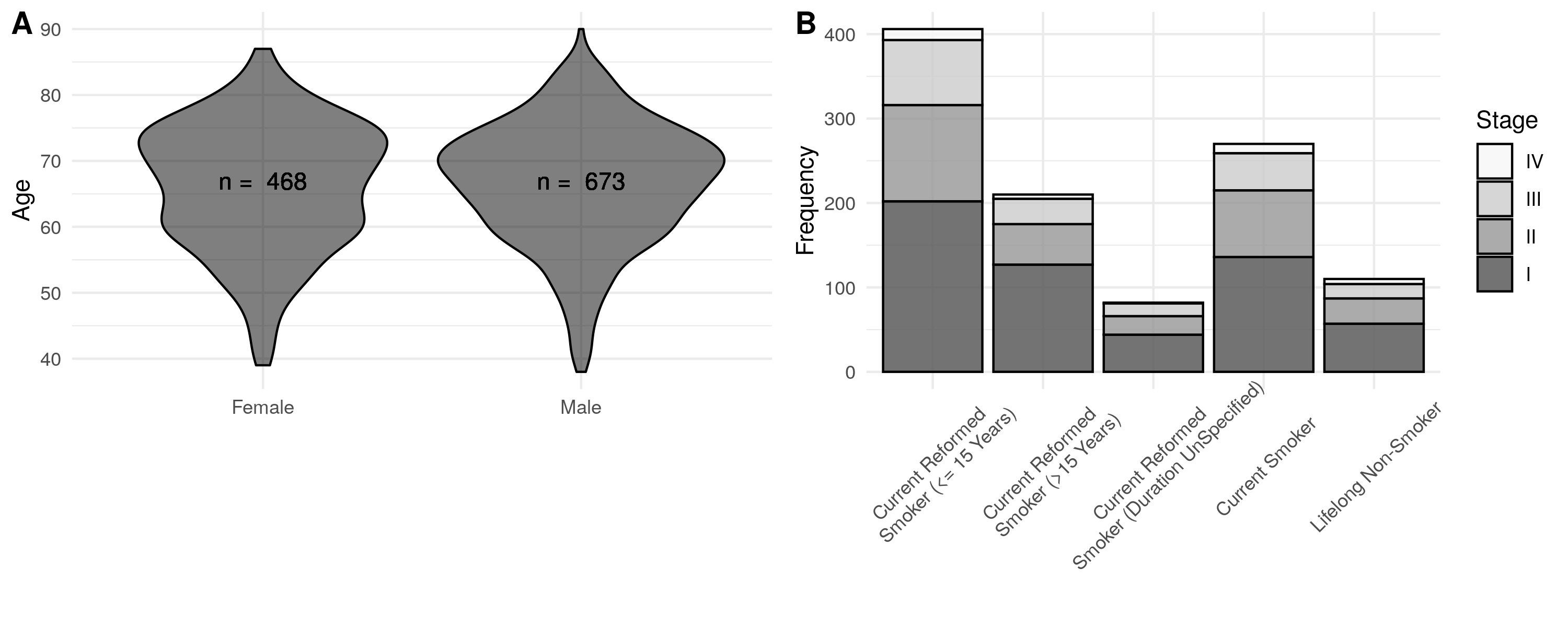
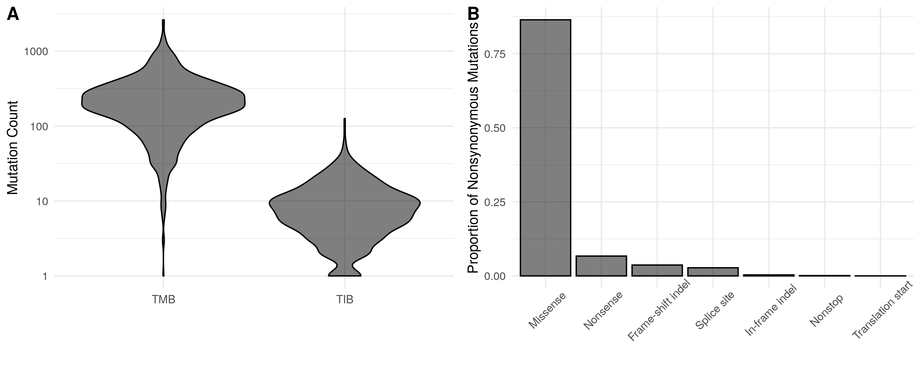
Our methodology can be applied to any annotated mutation dataset obtained by WES. To demonstrate our proposal we make use of the NSCLC dataset produced by campbell_distinct_2016, which contains data from 1144 patient-derived tumours. For each sample in this dataset we have the genomic locations and variant types of all mutations identified. At the time of the study, the patients had a variety of prognoses and smoking histories, were aged between 39 and 90, 41% were female and 59% were male; see Figure 1. In Figure 2A we see that mutations counts are distributed over a very wide range, as is the case in many cancer types (chalmers_analysis_2017). For simplicity, we only consider seven nonsynonymous variant types: missense mutations (which are the most abundant), nonsense mutations, frameshift insertions/deletions, splice site mutations, in-frame insertions/deletions, nonstop mutations and translation start site mutations. We present the frequencies of these mutation types in Figure 2B. Frameshift insertion/deletion (also known as indel) mutations are of particular interest when predicting TIB, but contribute only a small proportion ($<4\%$) of nonsynonymous mutations.

Figure 1: Demographic data for the clinical cohort in campbell_distinct_2016. A: Violin plots of age for patients, stratified by sex. B: Stacked bar chart of patients’ smoking histories, shaded according to cancer stage diagnosis.

Figure 2: Dataset-wide distribution of mutations. A: Violin plot of the distribution of TMB and TIB across training samples. B: The relative frequency of different nonsynonymous mutation types.

It is useful at this point to introduce the notation used throughout the paper. The set $G$ denotes the collection of genes that make up the exome. For a gene $g\in G$, let $\ell_{g}$ be the length of $g$ in nucleotide bases, defined by the maximum coding sequence. A gene panel is a subset $P\subseteq G$, and we write $\ell_{P}:=\sum_{g\in P}\ell_{g}$ for its total length. We let $S$ denote the set of variant types in our data (e.g. in the dataset mentioned above, $S$ contains the seven possible non-synonymous variants). Now, for $i=0,1,\ldots,n$, let $M_{igs}$ denote the count of mutations in gene $g\in G$ of type $s\in S$ in the $i$th sample. Here the index $i=0$ is used to refer to an unseen test sample for which we would like to make a prediction, while the indices $i=1,\ldots,n$ enumerate the samples in our training data set. In order to define the exome-wide biomarker of particular interest, we specify a subset of mutation types $\bar{S}\subseteq S$, and let

$$T_{i\bar{S}}:=\sum_{g\in G}\sum_{s\in\bar{S}}M_{igs},$$ (1)

for $i=0,\ldots,n$. For example, including all non-synonymous mutation types in $\bar{S}$ specifies $T_{i\bar{S}}$ as the TMB of sample $i$, whereas letting $\bar{S}$ contain only indel mutations gives TIB.

Our main goal is to predict $T_{0\bar{S}}$ based on $\{M_{0gs}:g\in P,s\in S\}$, where the panel $P\subseteq G$ has length $\ell_{P}$ satisfying some upper bound. When it is clear from context that we are referring to the test sample and a specific choice of biomarker (i.e. $\bar{S}$ is fixed), we will simply write $T$ in place of $T_{0\bar{S}}$.

2.2 Generative model

We now describe the main statistical model that underpins our methodology. In order to account for selective pressures and other factors within the tumour, we allow the rate at which mutations occur to depend on the gene and type of mutation. Our model also includes a sample-dependent parameter to account for the differing levels of mutagenic exposure of tumours, which may occur due to exogenous (e.g. UV light, cigarette smoke) or endogenous (e.g. inflammatory, free radical) factors.

We model the mutation counts $M_{igs}$ as independent Poisson random variables with mutation rates $\phi_{igs}>0$. More precisely, for $i=0,1,\ldots,n$, $g\in G$ and $s\in S$, we have

$$M_{igs}\sim\mathrm{Poisson}(\phi_{igs}),$$ (2)

where $M_{igs}$ and $M_{i^{\prime}g^{\prime}s^{\prime}}$ are independent for $(i,g,s)\neq(i^{\prime},g^{\prime},s^{\prime})$. Further, to model the dependence of the mutation rate on the sample, gene and mutation type, we use a log link function and let

$$\log(\phi_{igs})=\mu_{i}+\log(\ell_{g})+\lambda_{g}+\nu_{s}+\eta_{gs},$$ (3)

for $\mu_{i},\lambda_{g},\nu_{s},\eta_{gs}\in\mathbb{R}$, where for identifiability we set $\eta_{gs_{1}}=0$, for some $s_{1}\in S$ and all $g\in G$.

The terms in our model can be interpreted as follows. First, the parameter $\mu_{i}$ corresponds to the BMR of the $i$th sample. The offset $\log(\ell_{g})$ accounts for a mutation rate that is proportional to the length of a gene, so that a non-zero value of $\lambda_{g}$ corresponds to increased or decreased mutation rate relative to the BMR. The parameters $\nu_{s}$ and $\eta_{gs}$ account for differences in frequency between mutation types for each gene.

The model in (2) and (3) (discounting the unseen test sample $i=0$) has $n+|S|+|G||S|$ free parameters and we have $n|G||S|$ independent observations in the training data set. In principle we could attempt to fit our model directly using maximum likelihood estimation. However, we wish to exploit the fact that most genes do not play an active role in the development of a tumour, and will be mutated approximately according to the BMR. This corresponds to the parameters $\lambda_{g}$ and $\eta_{gs}$ being zero for many $g\in G$. We therefore include an $\ell_{1}$-penalisation term applied to the parameters $\lambda_{g}$ and $\eta_{gs}$ when fitting our model. We do not penalise the parameters $\nu_{s}$ or $\mu_{i}$ since we expect that different mutation types occur at different rates, and that the BMR is different in each sample.

Writing $\mu:=(\mu_{1},\ldots,\mu_{n})$, $\lambda:=(\lambda_{g}:g\in G)$, $\nu:=(\nu_{s}:s\in S)$ and $\eta:=(\eta_{gs}:g\in G,s\in S)$, and given training observations $M_{igs}=m_{igs}$, we let

$$\mathcal{L}(\mu,\lambda,\nu,\eta)=\sum_{i=1}^{n}\sum_{g\in G}\sum_{s\in S}\Bigl{(}\phi_{igs}-m_{igs}\log\phi_{igs}\Bigr{)}$$

be the negative log-likelihood of the model specified by (2) and (3). We then define

$$(\hat{\mu},\hat{\lambda},\hat{\nu},\hat{\eta})=\operatorname*{arg\,min}_{\mu,\lambda,\nu,\eta}\Bigl{\{}\mathcal{L}(\mu,\lambda,\nu,\eta)+\kappa_{1}\Bigl{(}\sum_{g\in G}|\lambda_{g}|+\sum_{g\in G}\sum_{s\in S}|\eta_{gs}|\Bigr{)}\Bigr{\}},$$ (4)

where $\kappa_{1}\geq 0$ is a tuning parameter that controls the number of non-zero components in $\hat{\lambda}$ and $\hat{\eta}$, which we choose using cross-validation (see Section 2.5 for more detail).

2.3 Proposed estimator

We now attend to our main goal of estimating a given exome-wide biomarker for the unseen test sample. Fix $\bar{S}\subseteq S$ and recall that we write $T=T_{0\bar{S}}$. We wish to construct an estimator of $T$ that only depends on the mutation counts in a gene panel $P\subset G$, subject to a constraint on $\ell_{P}$. To that end, we consider estimators of the form

$$T(w):=\sum_{g\in G}\sum_{s\in S}w_{gs}M_{0gs},$$

for $w\in\mathbb{R}^{|G|\times|S|}$. In the remainder of this subsection we explain how the weights $w$ are chosen to minimise the expected squared error of $T(w)$ based on the generative model in Section 2.2.

Of course, setting $w_{gs}=1$ for $g\in G$ and $s\in\bar{S}$ (and $w_{gs}=0$ otherwise) will give $T(w)=T$. However, our aim is to make predictions based on a concise gene panel. If, for a given $g\in G$, we have $w_{gs}=0$ for all $s\in S$, then $T(w)$ does not depend on the mutations in $g$ and therefore the gene does not need to be included in the panel. In order to produce a suitable gene panel (i.e. with many $w_{gs}=0$), we penalise non-zero components of $w$ when minimising the expected squared error. We define our final estimator via a refitting procedure, which improves the predictive performance by reducing the bias, and is also helpful when applying our procedure to panels with predetermined genes.

To construct our estimator, note that under our model in (2) we have $\mathbb{E}M_{0gs}=\mathrm{Var}(M_{0gs})=\phi_{0gs}$, and it follows that the expected squared error of $T(w)$ is

$$\mathbb{E}\bigl{[}\{T(w)-T\}^{2}\bigr{]} =\mathrm{Var}(T(w))+\mathrm{Var}(T)-2\mathrm{Cov}(T(w),T)+\bigl{[}\mathbb{E}\{T(w)-T\}\bigr{]}^{2}$$

$$=\sum_{g\in G}\sum_{s\in\bar{S}}(1-w_{gs})^{2}\phi_{0gs}+\sum_{g\in G}\sum_{s\in S\setminus\bar{S}}w_{gs}^{2}\phi_{0gs}$$

$$\hskip 150.0pt+\Bigl{(}\sum_{g\in G}\sum_{s\in S}w_{gs}\phi_{0gs}-\sum_{g\in G}\sum_{s\in\bar{S}}\phi_{0gs}\Bigr{)}^{2}.$$ (5)

This depends on the unknown parameters $\mu_{0},\lambda_{g},\nu_{s}$ and $\eta_{gs}$, the latter three of which are replaced by their estimates given in (4). It is also helpful to then rescale (2.3) as follows: write $\hat{\phi}_{0gs}=\ell_{g}\exp(\hat{\lambda}_{g}+\hat{\nu}_{s}+\hat{\eta}_{gs})$, and define

$$p_{gs}:=\frac{\hat{\phi}_{0gs}}{\sum_{g^{\prime}\in G}\sum_{s^{\prime}\in\bar{S}}\hat{\phi}_{0g^{\prime}s^{\prime}}}=\frac{\ell_{g}\exp(\hat{\lambda}_{g}+\hat{\nu}_{s}+\hat{\eta}_{gs})}{\sum_{g^{\prime}\in G}\sum_{s^{\prime}\in\bar{S}}\ell_{g^{\prime}}\exp(\hat{\lambda}_{g^{\prime}}+\hat{\nu}_{s^{\prime}}+\hat{\eta}_{g^{\prime}s^{\prime}})}.$$

Then let

$$f(w):=\sum_{g\in G}\sum_{s\in\bar{S}}p_{gs}(1-w_{gs})^{2}+\sum_{g\in G}\sum_{s\in S\setminus\bar{S}}p_{gs}w_{gs}^{2}+K(\mu_{0})\big{(}1-\sum_{g\in G}\sum_{s\in S}p_{gs}w_{gs}\big{)}^{2},$$

where $K(\mu_{0})=\exp(\mu_{0})\sum_{g\in G}\sum_{s\in\bar{S}}\ell_{g}\exp(\hat{\lambda}_{g}+\hat{\nu}_{s}+\hat{\eta}_{gs})$. Since $f$ is a rescaled version of the error in (2.3) (with the true parameters $\lambda,\nu,\eta$ replaced by the estimates $\hat{\lambda},\hat{\nu},\hat{\eta}$), we will choose $w$ to minimise $f(w)$.

Note that $f$ only depends on $\mu_{0}$ via the $K(\mu_{0})$ term, which can be interpreted as a penalty factor controlling the bias of our estimator. For example, we may insist that the squared bias term $(1-\sum_{g\in G}\sum_{s\in S}p_{gs}w_{gs})^{2}$ is zero by setting $K(\mu_{0})=\infty$. In practice, we propose to choose the penalty $K$ based on the training data; see Section 2.5.

At this point $f(w)$ is minimised by choosing $w$ to be such that $w_{gs}=1$ for all $g\in G,s\in\bar{S}$, and $w_{gs}=0$ otherwise. As mentioned above, in order to form a concise panel while optimising predictive performance, we impose a constraint on the cost of sequencing the genes used in the estimation. More precisely, for a given $w$, an appropriate cost is

$$\|w\|_{G,0}:=\sum_{g\in G}\ell_{g}\mathbbm{1}\{w_{gs}\neq 0\ \mathrm{for\ some\ }s\in S\}.$$

This choice acknowledges that the cost of a panel is roughly proportional to the length of the region of genomic space sequenced, and that once a gene has been sequenced for one mutation type there is no need to sequence again for other mutation types.

Now, given a cost restriction $L$, our goal is to minimise $f(w)$ such that $\|w\|_{G,0}\leq L$. In practice this problem is non-convex and so computationally infeasible. As is common in high-dimensional optimisation problems, we consider a convex relaxation as follows: let $\|w\|_{G,1}:=\sum_{g\in G}\ell_{g}\|w_{g}\|_{2}$, where $w_{g}=(w_{gs}:s\in S)\in\mathbb{R}^{|S|}$, for $g\in G$, and $\|\cdot\|_{2}$ is the Euclidean norm. Define

$$\hat{w}^{\text{first-fit}}\in\operatorname*{arg\,min}\limits_{w}\bigl{\{}f(w)+\kappa_{2}\|w\|_{G,1}\bigr{\}},$$ (6)

where $\kappa_{2}\geq 0$ is chosen to determine the size of the panel selected.

The final form of our estimator is obtained by a refitting procedure. First, for $P\subseteq G$, let

$$W_{P}:=\{w\in\mathbb{R}^{|G|\times|S|}:w_{g}=(0,\ldots,0)\ \ \text{for}\ \ g\in G\setminus P\}.$$ (7)

Let $\hat{P}:=\{g\in G:\ \|\hat{w}^{\text{first-fit}}_{g}\|_{2}>0\}$ be the panel selected by the first-fit estimator in (6), and define

$$\hat{w}^{\text{refit}}\in\operatorname*{arg\,min}\limits_{w\in W_{\hat{P}}}\bigl{\{}f(w)\bigr{\}}.$$ (8)

We then estimate $T$ using $\hat{T}:=T(\hat{w}^{\text{refit}})$, which only depends on mutations in genes contained in the selected panel $\hat{P}$. The performance of our estimator is investigated in Section 3, for comparison we also include the performance of the first-fit estimator $T(\hat{w}^{\mathrm{first-fit}})$.

2.4 Panel augmentation

In practice, when designing gene panels a variety of factors contribute to the choice of genes included. For example, a gene may be included due to its relevance to immune response or its known association with a particular cancer type. If this is the case, measurements for these genes will be made regardless of their utility for predicting exome-wide biomarkers. When implementing our methodology, therefore, there is no additional cost to incorporate observations from these genes into our prediction if they will be helpful. Conversely researchers may wish to exclude genes from a panel, or at least from actively contributing to the estimation of a biomarker, for instance due to technical difficulties in sequencing a particular gene.

We can accommodate these restrictions by altering the structure of our regularisation penalty in (6). Suppose we are given (disjoint sets of genes) $P_{0},Q_{0}\subseteq G$ to be included and excluded from our panel, respectively. In this case, we replace $\hat{w}^{\text{first-fit}}$ in (6) with

$$\hat{w}_{P_{0},Q_{0}}^{\text{first-fit}}\in\operatorname*{arg\,min}\limits_{w\in W_{G\setminus Q_{0}}}\bigl{\{}f(w)+\kappa_{2}\sum_{g\in G\setminus P_{0}}l_{g}\|w_{g}\|_{2}\bigr{\}}.$$ (9)

Excluding the elements of $P_{0}$ from the penalty term means that $\hat{w}_{P_{0},Q_{0}}^{\text{first-fit}}\neq 0$ for the genes in $P_{0}$, while restricting our optimisation to $W_{G\setminus Q_{0}}$ excludes the genes in $Q_{0}$ by definition. This has the effect of augmenting the predetermined panel $P_{0}$ with additional genes selected to improve predictive performance. We then perform refitting as described above. We demonstrate this procedure by augmenting the TST-170 gene panel in Section LABEL:sec:augmentation.

2.5 Practical considerations

In this section, we discuss some practical aspects of our proposal. Our first consideration concerns the choice of the tuning parameter $\kappa_{1}$ in $\eqref{eq:genparams}$. As is common for the Least Absolute Shrinkage and Selection Operator (LASSO) estimator in generalised linear regression (see, for example, michoel_natural_2016 and friedman_glmnet_2021), we will use 10-fold cross-validation. To highlight one important aspect of our cross-validation procedure, recall that we consider the observations $M_{igs}$ as independent across the sample index $i\in\{1,\ldots,n\}$, the gene $g\in G$ and the mutation type $s\in S$. Our approach therefore involves splitting the entire set $\{(i,g,s):i=1,\ldots,n,g\in G,s\in S\}$ of size $n|G||S|$ (as opposed to the sample set $\{1,\ldots,n\}$) into 10 folds uniformly at random. We then apply the estimation method in (4) to each of the 10 folds separately on a grid of values (on the log scale) of $\kappa_{1}$, and select the value that results in the smallest average deviance across the folds. The model is then refitted using all the data for this value of $\kappa_{1}$.

The estimated coefficients in (6) depend on the choice of $K(\mu_{0})$ and $\kappa_{2}$. As mentioned above, we could set $K(\mu_{0})=\infty$ to give an unbiased estimator, however in practice we found that a finite choice of $K(\mu_{0})$ leads to improved predictive performance. Our recommendation is to use $K(\mu_{0})=K(\max_{i=1,\ldots,n}\{\hat{\mu}_{i}\})$, where $\hat{\mu}_{i}=\log(T_{i}/\sum_{g,s}\ell_{g}\exp(\hat{\lambda}_{g}+\hat{\nu}_{s}+\hat{\eta}_{gs}))$ is a pseudo-MLE (in the sense of gong_pseudo_1981) for $\mu_{i}$, so that the penalisation is broadly in proportion with the largest values of $\mu_{i}$ in the training dataset. The tuning parameter $\kappa_{2}$ controls the size of the gene panel selected in (6): given a panel length $L$, we set $\kappa_{2}(L)=\max\{\kappa_{2}:\ \ell_{\hat{P}}\leq L\}$ in order to produce a suitable panel.

We now comment briefly on some computational aspects of our method. The generative model fit in (4) can be solved via coordinate descent (see, for example, friedman_regularization_2010), which has a computational complexity of $O(N|G|^{2}|S|^{2})$ per iteration. We fit the model 10 times, one for each fold in our cross-validation procedure. This is the most computationally demanding part of our proposal – in our experiments below, it takes approximately an hour to solve on a standard laptop – but it only needs to be carried out once for a given dataset. The convex optimisation problem in (6) can be solved by any method designed for the group LASSO; see, for example, yang_fast_2015. In our experiments in Section 3, we use the gglasso R package (yang_gglasso_2020), which takes around 10 minutes to reproduce the plot in Figure LABEL:fig:6. Note also that the solutions to (6) and (8) are unique; see, for example, roth_group-lasso_2008. The last step of our proposal, namely making predictions for new test observations based on a selected panel, carries negligible computational cost.

Finally we describe a heuristic procedure for producing prediction intervals around our point estimates. In particular, for a given confidence level $\alpha\in(0,1)$, we aim to find an interval $[\hat{T}_{\mathrm{L}},\hat{T}_{\mathrm{U}}]$ such that $\mathbb{P}\bigl{(}\hat{T}_{\mathrm{L}}\leq T\leq\hat{T}_{\mathrm{U}}\bigr{)}\geq 1-\alpha.$ To that end, let $t_{\alpha}:=\mathbb{E}\{(\hat{T}-T)^{2}\}/\alpha$, then by Markov’s inequality we have that $\mathbb{P}(|\hat{T}-T|^{2}\geq t_{\alpha})\leq\alpha$. It follows that $[\hat{T}-t_{\alpha}^{1/2},\hat{T}+t_{\alpha}^{1/2}]$ is a $(1-\alpha)$-prediction interval for $T$. Of course, the mean squared error $\mathbb{E}\{(\hat{T}-T)^{2}\}$ defined in (2.3) depends on the parameters $\lambda,\eta,\nu$ and $\mu_{0}$, which are unknown. Our approach is to utilise the estimates $\hat{\lambda},\hat{\eta},\hat{\nu}$ (see (4)) and replace $\mu_{0}$ with $\log(\hat{T}/\sum_{g,s}\ell_{g}\exp(\hat{\lambda}_{g}+\hat{\nu}_{s}+\hat{\eta}_{gs}))$. While this is not an exact $(1-\alpha)$-prediction interval for $T$, we will see in our experimental results in Sections 3.2 and LABEL:sec:indel that in practice this approach provides intervals with valid empirical coverage.

3 Demonstration using an NSCLC dataset

In this section we demonstrate the practical performance of our proposal using the dataset from campbell_distinct_2016, which we introduced in Section 2.1. Our main focus is the prediction of TMB, and we show that our approach outperforms the state-of-the-art approaches. We also analyse the suitability of our generative model, consider the task of predicting the recently proposed biomarker TIB, and include a panel augmentation case study with the TST-170 gene panel.

Since we are only looking to produce estimators for TMB and TIB, we group mutations into two categories – indel mutations and all other non-synonymous mutations – so that $|S|=2$. This simplifies the presentation of our results and reduces the computational cost of fitting the generative model. In order to assess the performance of each of the methods in this section, we randomly split the dataset into training, validation and test sets, which contain $n_{\text{train}}=n=800,\ n_{\text{val}}=171$ and $n_{\text{test}}=173$ samples, respectively. Mutations are observed in $|G|=17358$ genes. Our training set comprises samples with an average TMB of $252$ and TIB of $9.25$.

3.1 Generative model fit and validation

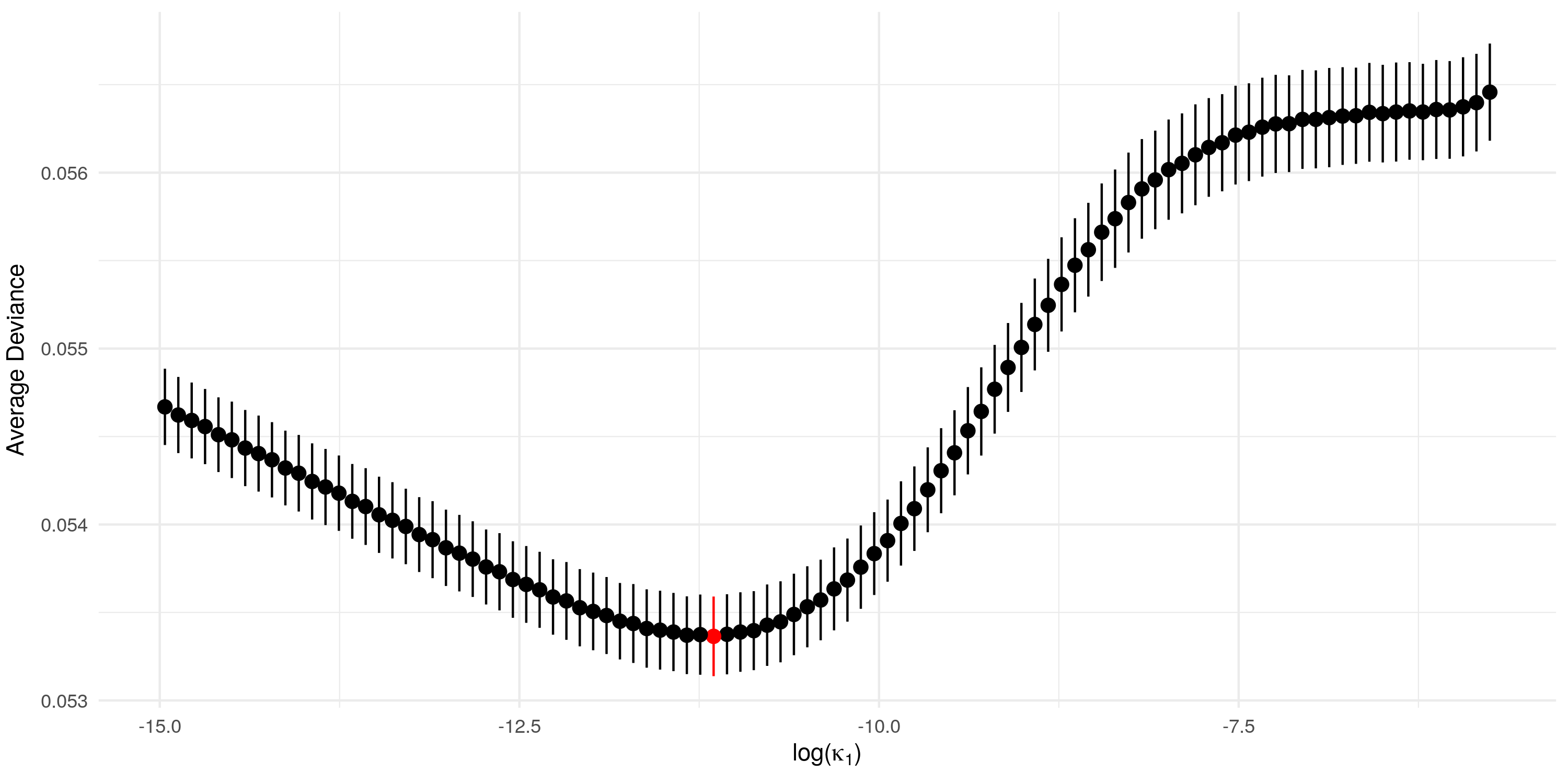
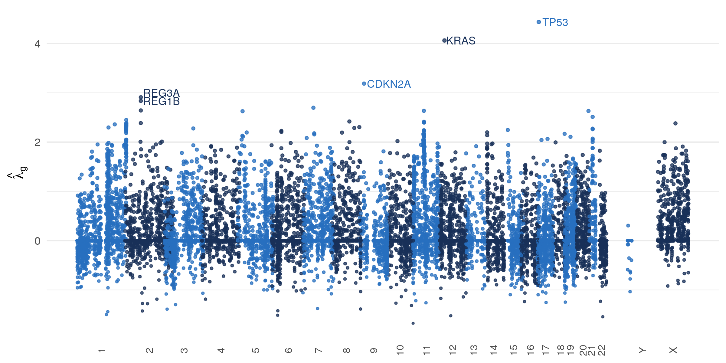
The first step in our analysis is to fit the model proposed in Section 2.2 using only the training dataset. In particular, we obtain estimates of the model parameters using equation (4), where the tuning parameter $\kappa_{1}$ is determined using 10-fold cross-validation as described in Section 2.5. The results are presented in Figure 3. The best choice of $\kappa_{1}$ produces estimates of $\lambda$ and $\eta$ with $44.4\%$ and $77.8\%$ sparsity respectively, i.e. that proportion of their components are estimated to be exactly zero. We plot $\hat{\lambda}$ and $\hat{\eta}$ for this value of $\kappa_{1}$ in Figures 4 and 5. Genes with $\hat{\lambda}_{g}=0$ are interpreted to be mutating according to the background mutation rate, and genes with $\hat{\eta}_{\text{g,indel}}=0$ are interpreted as having no specific selection pressure for or against indel mutations. In Figures 4 and 5 we highlight genes with large (in absolute value) parameter estimates, some of which have known biological relevance in oncology; see Section LABEL:sec:conclusion for further discussion. Finally, note that the average $\mu_{i}$ among current smokers is 5.40 (with standard deviation 0.76), amongst reformed smokers is 5.26 (0.84), and among lifelong non-smokers is 4.04 (1.12). This suggest that smokers may have higher BMR s, which is as we expect.

Figure 3: The average deviance (with one standard deviation) across the 10 folds in our cross-validation procedure plotted against $\log(\kappa_{1})$. The minimum average deviance is highlighted red.

Figure 4: Manhattan plot of fitted parameters $\hat{\lambda}_{g}$ and their associated genes’ chromosomal locations. The genes with the five largest positive parameter estimates are labelled.

Figure 5: Manhattan plot of fitted parameters $\hat{\eta}_{g,\text{indel}}$ and their associated genes’ chromosomal locations. The five largest positive and negative genes are labelled.

We now validate our model in (3) by comparing with the following alternatives:

1. Saturated model: the model in (2), where each observation has an associated free parameter (i.e. $\phi_{igs}>0$ is unrestricted);

2. No sample-specific effects: the model in (3), with $\mu_{i}=0$ for all $i\in\{1,\ldots,n\}$;

3. No gene-specific effects: the model in (3), with $\lambda_{g}=\eta_{gs}=0$ for all $g\in G$ and $s\in S$;

4. No gene/mutation type interactions: the model in (3), with $\eta_{gs}=0$ for all $g\in G$ and $s\in S$.

In Table 1 we present the residual deviance and the residual degrees of freedom between our model and each of the models above. We see that our model is preferred over the saturated model, and all three submodels of (3).

Table 1: Model comparisons on the basis of residual deviance statistics.

Comparison	Residual	Residual Degrees	dev/df	$p$-value
Model	Deviance (dev)	of Freedom (df)
(i)	$1.43\times 10^{6}$	$2.74\times 10^{7}$	$1.00$
(ii)	$1.42\times 10^{5}$	$8.00\times 10^{2}$	$1.77\times 10^{2}$	$0.00$
(iii)	$1.10\times 10^{5}$	$1.33\times 10^{4}$	$8.24\times 10^{0}$	$0.00$
(iv)	$1.70\times 10^{4}$	$1.82\times 10^{3}$	$9.33\times 10^{0}$	$0.00$

3.2 Predicting tumour mutation burden

We now demonstrate the excellent practical performance of our procedure for estimating