Eddy memory as an explanation of intra-seasonal periodic behavior in baroclinic eddies

Abstract

The baroclinic annular mode (BAM) is a leading-order mode of the eddy-kinetic energy in the Southern Hemisphere exhibiting oscillatory behavior at intra-seasonal time scales. The oscillation mechanism has been linked to transient eddy-mean flow interactions that remain poorly understood. Here we demonstrate that the finite memory effect in eddy-heat flux dependence on the large-scale flow can explain the origin of the BAM’s oscillatory behavior. We represent the eddy memory effect by a delayed integral kernel that leads to a generalized Langevin equation for the planetary-scale heat equation. Using a mathematical framework for the interactions between planetary and synoptic scale motions, we derive a reduced dynamical model of the BAM – a stochastically-forced oscillator with a period proportional to the geometric mean between the eddy-memory time scale and the diffusive eddy equilibration timescale. Our model provides a formal justification for the previously proposed phenomenological model of the BAM and could be used to explicitly diagnose the memory kernel and improve our understanding of transient eddy-mean flow interactions in the atmosphere.

I Introduction

Large-scale atmospheric dynamics at mid-latitudes is significantly influenced by the baroclinic wave life cycle initiated by shear instability (Pierrehumbert and Swanson, 1995). Constrained by geostrophic and hydrostatic balance, a meridional temperature gradient imposed by the heat imbalance between tropics and high latitudes is proportional to the vertical shear of the mid-latitude jet, which acts as a key parameter controlling the growth rate of baroclinic waves (Charney, 1947; Eady, 1949; Phillips, 1951). During the baroclinic growth of synoptic waves, poleward heat flux increases and the waves propagate upward, after which the waves break near critical latitudes while propagating equatorward. The whole life cycle of unstable baroclinic waves could be represented by energy exchange between zonal mean zonal wind and synoptic eddies (Lorenz, 1955; Simmons and Hoskins, 1978; Edmon Jr et al., 1980; Moon and Feldstein, 2009). This cycle is reflected in daily weather at mid-latitudes and understood as an engine to transfer residual energy from the tropics to high latitudes. It determines many aspects of large-scale circulations in extra-tropical areas (Held and Hoskins, 1985).

The life cycle of baroclinic waves is an essential part of variability in mid-latitudes with its time-scale being around 3-4 days. However, the low-frequency intra-seasonal variability with a time scale longer than weather but shorter than seasonal (Branstator, 1992; Hartmann, 1974) is not entirely explained by the traditional baroclinic wave life cycle (Pratt, 1977; Barnston and Livezey, 1987). For example, the North Atlantic Oscillation (NAO) (Hurrell et al., 2003), which represents the fluctuation of the difference of atmospheric pressure between the Icelandic Low and the Azores High, contains the intra-seasonal time-scale of around 10-days. Similarly, the Arctic Oscillation (AO) (Thompson and Wallace, 1998) or the Southern Annular Mode (SAM) (Limpasuvan and Hartmann, 1999), representing the zonally symmetric seesaw between sea level pressures in polar and temperate latitudes in Northern and Southern Hemisphere, respectively, also vary on intra-seasonal timescales.

The variability of the mid-latitude westeries is commonly defined using the zonal index (Namias, 1950) that was originally defined by the pressure difference between 35N and 55N, but there are many variants (Robinson, 1996; Li and Wang, 2003). The zonal index, especially in the Southern Hemisphere, shows strong intraseasonal and interannual variability based on several observational data (Hartmann and Lo, 1998). On intra-seasonal time-scales, it is hard to identify a major external forcing and hence the mid-latitude jet variability could be controlled by internal dynamics (Branstator, 1992). Indeed, the low-frequency variability of the zonal index has been identified in simple numerical models with zonally-symmetric thermal forcing (Robinson, 1991), implying that variability can be caused by the interaction between synoptic eddies and zonal mean field.

The eddy-mean flow interaction is a highly nonlinear process involving turbulent mixing of synoptic waves leading to energy transfer among different scales that are difficult to accurately parameterize. However, phenomenological models of eddy-mean flow interactions exhibiting oscillatory behavior have been put forward. Thompson and Barnes (2014) introduced a stochastic model to explain the quasi-oscillatory behavior of the poleward heat flux in the Southern Hemisphere, also referred to as the Southern Hemisphere baroclinic annular mode (BAM) introuduced by Thompson and Woodworth (2014). Specifically, they suggest a two-dimensional stochastic model representing interactions between the poleward heat flux and the meridional temperature gradient to capture the quasi-oscillatory variability with a dominant time-period around 25 days. In this model, the increase of the poleward heat flux is proportional to the growth rate of eddies generated by baroclinic instability, which is proportional to the meridional temperature gradient. At the same time, the time evolution of the anomalous meridional temperature gradient is controlled by the poleward heat flux with a damping. This phenomenology results in a two-dimensional stochastic dynamical system that contains oscillatory solutions depending on the choice of parameters. With this idealized description of the variability, Thompson and Barnes (2014) suggest that the quasi-oscillatory low-frequency variability can be caused by nonlinear eddy-mean flow interaction. Even though the model reflects the basic characteristics of the baroclinic wave life cycle, its direct connection to the primitive equations is not described, which obscures the physical interpretation of model parameters.

The BAM is a companion index of the Southern Annular mode (SAM) in the Southern Hemisphere representing the characteristics of large-scale low frequencies in the atmosphere. The SAM is defined by zonal mean kinetic energy describing the variability of zonal mean wind mainly influenced by the momentum flux. The BAM is constructed by eddy kinetic energy mainly controlled by the meridional heat flux in lower levels (Thompson and Woodworth, 2014). The two processes, meridional heat flux in lower levels and momentum flux in upper ones, show different characteristics in their variabilities (Boljka and Shepherd, 2018; Boljka et al., 2018; Wang and Nakamura, 2015, 2016; Pfeffer, 1992). The SAM is well approximated by an autoregressive model of order 1 (AR(1) process), having a red noise spectrum, but the BAM shows a distinct peak around 25 days in its power spectrum. The stochastic oscillatory behavior shown in the BAM is worthwhile to be investigated in detail due to the expectation that it leads to significant progress in predictability in mid-latitudes on sub-seasonal time-scales. Furthermore, Thompson and Li (2015) argue that the BAM in the Northern Hemisphere shows a dominant peak located at around 20 days in its power spectrum. This implies that the oscillatory behavior in meridional heat flux or eddy kinetic energy is an intrinsic feature of eddy-mean flow interactions in large-scale atmospheric dynamics. Therefore, the major question is how the meridional heat flux in lower levels can induce the oscillatory behavior in the interaction with mean field.

Generation of low-frequency oscillations in a rotating fluid does not seem to be limited to the large-scale atmosphere as similar internal oscillations were also found in large-scale ocean currents. An eddy-resolving ocean model simulation with a repeated annual cycle forcing reveals an intrinsic mode in the Southern Ocean with a period of 40-50 year (Le Bars et al., 2016; van Westen and Dijkstra, 2017). An idealized model of the surface-stress-driven Beaufort Gyre in the Arctic Ocean with mesoscale eddies as a key equilibration process (Manucharyan and Spall, 2016) generates an oscillation with a period of 50 years (Manucharyan et al., 2017). To explain the oscillation Manucharyan et al. (2017) introduce eddy memory into the relation between the eddy buoyancy flux and the mean buoyancy gradient, which leads to a modification of the commonly used Gent-McWilliams (GM) parameterization (Gent and McWilliams, 1990). The inclusion of eddy memory leads to a stochastic oscillation if the ratio between the memory timescale and the diffusive equilibration timescale reaches a certain threshold (Manucharyan et al., 2017).

Generally, according to the Mori-Zwanzig formalism (Zwanzig, 1961), the dynamic interactions between slow-evolving modes and fast ones are reflected as a delayed integral on the time evolution of the slowly-varying modes. The memory effect, normally represented by a delayed term or integral, is not new in climate science. One of the simplest models for the El-Ninõ and Southern Oscillation (ENSO) is a delayed ordinary differential equation (Suarez and Schopf, 1988). Even with such one-dimensional model, it was found that the delayed model contains chaotic dynamics under seasonal forcing(Tziperman et al., 1994). Recently, such delay equation climate models were derived using the Mori-Zwanzig formalism (Falkena et al., 2019). Considering the complex interactions in fluid-dynamical systems, the memory effect is an intrinsic characteristic leading to various internal variability.

Our research focuses on the memory effect in the interaction between synoptic eddies and a zonal mean zonal wind and its relation to low frequency modes on timescales longer than the weather. More specifically, we propose a formalized explanation of the quasi-oscillatory behavior of the BAM (Thompson and Barnes, 2014) by incorporating the eddy memory (Manucharyan et al., 2017) into multi-scale equations of atmospheric dynamics (Moon and Cho, 2020). We outline the multi-scale atmospheric model in Section II and we introduce the eddy memory effect onto the planetary -scale equations in Section 3., where we formally derive the reduced model for the zonal mean flow, the stochastic oscillator. We conclude in Section 4.

II Multiscale model of atmospheric motions

The basic governing equation for Earth’s climate starts from the simplest heat flux balance between short-wave radiative flux and outgoing longwave radiative flux, which gives us a global average temperature as an equilibrium. This is possible when we consider the Earth as a point object in the universe maintaining a thermal equilibrium state. If we magnify the size of the Earth from a point to a sphere, we can see that there is an imbalance of heat flux from tropics to higher latitudes, which requires transferring heat from the tropics to higher latitudes. A simple approximation of the poleward heat flux is a turbulent diffusion with a constant eddy diffusivity. In an even more magnified view of the tropics and polar areas, the dominant physics shifts from energy flux balance to potential vorticity conservation, which acts as a theoretical foundation for the generation of mid-latitude weather systems. There are unclearly defined timescales between the weather dominated by the vorticity dynamics and the season controlled by external heat flux. These timescales lie on around 10 to 30 days, where numerous variability has been detected in climate data. There should be an intermediate framework lying between the energy flux balance and the vorticity dynamics to investigate causes of the variability.

The large-scale atmosphere is governed by the primitive equations which are comprised of three momentum balances, the continuity equation and the heat budget. In Cartesian coordinates, the three momentum equations are

$$\frac{Du}{Dt}-fv=-\frac{1}{\rho}\frac{\partial P}{\partial x}$$

$$\frac{Dv}{Dt}+fu=-\frac{1}{\rho}\frac{\partial P}{\partial y}$$

$$\frac{Dw}{Dt}=-\frac{1}{\rho}\frac{\partial P}{\partial z}-g,$$ (1)

where $P$ and $\rho$ are atmospheric pressure and density, respectively, and the velocities in the zonal, meridional, and vertical directions are $u$, $v$, and $w$. The Coriolis parameter $f$ is approximated by $f_{0}+\beta y$, where $f_{0}$ is a Coriolis parameter calculated at a reference latitude $\phi_{0}$ and $\beta y$ is the latitudinal variation of the Coriolis parameter where $\beta=\partial f/\partial y$. The material derivative $D/Dt$ is defined as $D/Dt\equiv\partial/\partial t+u\partial/\partial x+v\partial/\partial y+w\partial/\partial z$. Along with the momentum equations, the continuity equation is

$$\frac{1}{\rho}\frac{D\rho}{Dt}+\frac{\partial u}{\partial x}+\frac{\partial v}{\partial y}+\frac{\partial w}{\partial z}=0.$$ (2)

Finally, to complete the equations, we need the ideal gas law $P=\rho RT$ and thermodynamic equation

$$\frac{D\Theta}{Dt}=\frac{\Theta}{C_{P}T}\left(\frac{\kappa}{\rho}\nabla^{2}T+Q\right),$$ (3)

where $\Theta$ is the potential temperature, i.e.,

$$\Theta\equiv T\left(\frac{P_{00}}{P}\right)^{R/C_{P}},$$ (4)

where $P$ and $T$ represent the pressure and the temperature, respectively, $P_{00}$ is a reference pressure, typically $1000$mb, $R$ is the gas constant for air, $C_{P}$ the specific heat at the constant pressure, and $P_{00}$ is a reference pressure. The full equations are highly nonlinear and complicated and to explain the BAM, we need to simplify the equations using an appropriate scaling.

The scale of atmospheric motions is distinguished by the magnitude of the Rossby number, $U/fL$, where $U$ is a horizontal velocity scale, and $L$ is a horizontal length scale. When the Rossby number is asymptotically small, the geostrophic balance becomes a dominant force balance in the horizontal momentum equations. The large-scale atmospheric flows satisfying the geostrophic and hydrostatic balances are called geostrophic motions.

There are two kinds of geostrophic motions depending on the horizontal length scale (Phillips, 1963). If the length scale is similar to the internal Rossby deformation radius ($L\sim 1000km$), the motion is called quasi-geostrophic and is described by the conservation of potential vorticity,

$$\frac{{\rm D}_{H}}{{\rm D}t}\left[\frac{\partial^{2}\psi}{\partial x^{2}}+\frac{\partial^{2}\psi}{\partial y^{2}}+\frac{1}{\rho_{s}}\frac{\partial}{\partial z}\left(\frac{\rho_{s}}{S}\frac{\partial\psi}{\partial z}\right)+\beta y\right]\ =0,$$ (5)

where

$$\frac{{\rm D}_{H}}{{\rm D}t}=\frac{\partial}{\partial t}-\frac{\partial\psi}{\partial y}\frac{\partial}{\partial x}+\frac{\partial\psi}{\partial x}\frac{\partial}{\partial y},$$ (6)

$\psi$ is a leading-order pressure field acting as a stream function, $\rho_{s}$ is a mean vertical density profile, $S$ represents the average vertical stability, and $\frac{\partial^{2}\psi}{\partial x^{2}}+\frac{\partial^{2}\psi}{\partial y^{2}}+\frac{1}{\rho_{s}}\frac{\partial}{\partial z}\left(\frac{\rho_{s}}{S}\frac{\partial\psi}{\partial z}\right)+\beta y$ is the potential vorticity. All the variables are non-dimensionalized (Pedlosky, 2013). On the other hand, if the horizontal length-scale is close to the external Rossby deformation radius ($L_{D}\sim 3000km$), the governing equations become

$$u_{L}\ =\ -\frac{\partial P_{L}}{\partial y}$$ (7)

$$v_{L}\ =\ \frac{\partial P_{L}}{\partial x}$$ (8)

$$\rho_{L}\ =\ -\frac{1}{\rho_{s}}\frac{\partial}{\partial z}\Big{(}\rho_{s}P_{L}\Big{)}$$ (9)

$$\frac{1}{\rho_{s}}\frac{\partial}{\partial z}\Big{(}\rho_{s}w_{L}\Big{)}-\beta_{L}v_{L}\ =\ 0$$ (10)

$$\frac{\partial\Theta_{L}}{\partial t}+u_{L}\frac{\partial\Theta_{L}}{\partial x}+v_{L}\frac{\partial\Theta_{L}}{\partial y}+w_{L}\frac{\partial\Theta_{L}}{\partial z}+\frac{w_{L}}{\epsilon\Theta_{s}}\frac{{\rm d}\Theta_{s}}{{\rm d}z}\ =\ Q_{L},$$ (11)

where $P_{L}$ is the planetary-scale pressure, $u_{L}$, $v_{L}$ and $w_{L}$ are the zonal, the meridional and the vertical velocity, respectively, $\Theta_{s}$ is the hemispheric average potential temperature, $\Theta_{L}$ is an anomalous potential temperature, $\beta_{L}$ is the planetary-scale beta effect, and $Q_{L}$ represents radiative processes. The thermodynamic forcing $Q_{L}$ is a residual of local radiative fluxes driving a local temperature change. The subscript $L$ implies planetary-scale variables. Eqs. (7)-(11) are usually referred to as planetary geostrophy, where the heat equation with advection is constrained by the geostrophic and hydrostatic balances, together with the Sverdrup relation (Moon and Cho, 2020). Similar results can be found in Dolaptchiev and Klein (2009, 2013), where the same leading-order equations are derived. They used a different small parameter $\epsilon=(a\Omega^{2}/g)^{3}$ instead of the Rossby number $U/fL$, where $a$ is the earth’s radius and $\Omega$ is the earth’s rotation frequency, thus the detailed derivations toward the leading-order equations are different. On the other hand, Moon and Cho (2020) derive the same results based on the Rossby number as a small parameter in the asymptotic analysis following the historical development of theories of quasi-geostrophic motions in large-scale atmospheric dynamics (Pedlosky, 2013).

The two geostrophic motions coexist in the large-scale atmosphere. Hence, the large-scale atmospheric dynamics should be represented by interactions between the two scales. Because these two scales are asymptotically separate, we can use a multi-scale analysis in spatial and temporal domains. Based on the Rossby number in the planetary scale $\epsilon=U/(f_{0}L_{D})$, we can introduce the two scales, $(X,Y,\tilde{t})$ for the planetary scale and $(x,y,t)$ for the quasi-geostrophic (QG) one, where $(x,y,t)=\epsilon^{1/2}(X,Y,\tilde{t})$. Thus, the time and spatial derivatives are scaled as

$$\frac{\partial}{\partial t} \ \rightarrow\ \frac{\partial}{\partial\tilde{t}}+\epsilon^{-1/2}\frac{\partial}{\partial t}$$

$$\frac{\partial}{\partial x} \ \rightarrow\ \frac{\partial}{\partial X}+\epsilon^{-1/2}\frac{\partial}{\partial x}$$

$$\frac{\partial}{\partial y} \ \rightarrow\ \frac{\partial}{\partial Y}+\epsilon^{-1/2}\frac{\partial}{\partial y}\,.$$

The two scales are separated by $\epsilon^{1/2}$ which comes from the estimation that $L/L_{D}\sim\epsilon^{1/2}$ in the large-scale atmosphere in the earth. The internal Rossby deformation radius $L$ is around $1000$km in mid-latitudes and the external (barotropic) one $L_{D}$ around $3000$km.

A regular perturbation analysis of the primitive equations (1-4) (Moon and Cho, 2020) leads to

$$u_{L}=-\frac{\partial P_{L}}{\partial Y},\quad v_{L}=\frac{\partial P_{L}}{\partial X},\quad\rho_{L}=-\frac{1}{\rho_{s}}\frac{\partial}{\partial z}\left(\rho_{s}P_{L}\right)$$ (12)

$$u_{0}=-\frac{\partial P_{0}}{\partial y},\quad v_{0}=\frac{\partial P_{0}}{\partial x},\quad\rho_{0}=-\frac{1}{\rho_{s}}\frac{\partial}{\partial z}\left(\rho_{s}P_{0}\right)$$ (13)

$$\frac{\partial w_{L}}{\partial z}-\frac{1}{H}w_{L}\ =\ \beta_{L}v_{L}$$ (14)

$$\frac{\partial\Theta_{L}}{\partial\tilde{t}}+u_{L}\frac{\partial\Theta_{L}}{\partial X}+v_{L}\frac{\partial\Theta_{L}}{\partial Y}+w_{L}\left(\frac{\partial\Theta_{L}}{\partial z}+S\right)\ =\$$

$$\ -\left(\frac{\partial}{\partial t}+u_{L}\frac{\partial}{\partial x}+v_{L}\frac{\partial}{\partial y}\right)\Theta_{0}-\left(u_{0}\frac{\partial}{\partial X}+v_{0}\frac{\partial}{\partial Y}\right)\Theta_{L}$$

$$-\frac{\partial}{\partial x}\Big{(}u_{0}\Theta_{0}\Big{)}-\frac{\partial}{\partial y}\Big{(}v_{0}\Theta_{0}\Big{)}-w_{1}\left(\frac{\partial\Theta_{L}}{\partial z}+S\right)+Q_{L}$$ (15)

$$\frac{\partial}{\partial t}\nabla^{2}P_{0}+(u_{L}+u_{0})\frac{\partial}{\partial x}\nabla^{2}P_{0}+(v_{L}+v_{0})\frac{\partial}{\partial y}\nabla^{2}P_{0}+\beta v_{0}$$

$$\quad=\left(\frac{\partial}{\partial z}-\frac{1}{H}\right)w_{1}\ ,$$ (16)

where $\frac{1}{H}=-\frac{1}{\rho_{s}}\frac{d\rho_{s}(z)}{dz}$ and $S=\frac{1}{F\Theta_{s}}\frac{d\Theta_{s}(z)}{dz}$. The Burger number $F$ is defined as $L^{2}/L^{2}_{D}$ where $L$ is an internal Rossby number and $L_{D}$ the external Rossby number. These $L$ and the numbers $0$ and $1$ are used as the subscripts to represent planetary-scale and synoptic-scale variables, respectively. The number $0$ (the number $1$) represents the leading-order (the next order) in the synoptic-scale. It is assumed that planetary-scale (synoptic-scale) variables are only dependent upon planetary-scale (synoptic-scale) coordinates, $X$, $Y$, and $\tilde{t}$ ($x$, $y$, and $t$). The vertical coordinate $z$ is used for the both scales. The equations (12-16) show the dynamics of the two scales and their mutual interactions. The detailed derivation and discussions are found in Moon and Cho (2020). The equations (12-14) describe that the two scales satisfy the basic balances, geostrophic and hydrostatic balances. The continuity equation (14) in the planetary scale includes the $O(1)$ beta effect, which is known as the Sverdrup relation. The two scales contribute to the energy flux balance in the heat equation (15) with their own temporal and spatial scales. The last equation (16) is the vorticity equation governing the quasi-geostrophic dynamics. Here the planetary geostrophic motion provides a mean field for the development of vorticity on the Rossby deformation scale. Dolaptchiev and Klein (2013) also considered a similar multi-scale analysis to represent the interactions between planetary and synoptic scales, which leads to equivalent results. However, their main focus lies on vorticity dynamics at the two scales, and hence a planetary vorticity equation is derived from the combination of the heat equation and the Sverdrup relation along with the quasi-geostrophic potential vorticity equation. Our focus is in the planetary-scale heat equation with thermal forcing $Q_{L}$. Lying between the simple energy flux balance model (North et al., 1981) and the quasi-geostrophic dynamics, the planetary heat equation together with basic dynamic balances connects the planetary thermal heat flux to fluid dynamics on planetary scales.

The above equations become simpler when the planetary-scale thermodynamic forcing $Q_{L}$ is zonally homogeneous. The planetary scale preserves that symmetry, in which case all $X$-derivative terms vanish. Hence, the zonal means of the planetary meridional and vertical velocities $v_{L}$ and $w_{L}$ become zero. This yields

$$u_{L}\ =\ -\frac{\partial P_{L}}{\partial Y}$$ (17)

$$\frac{\partial\Theta_{L}}{\partial\tilde{t}}\ =\ -\left(\frac{\partial}{\partial t}+u_{L}\frac{\partial}{\partial x}\right)\Theta_{0}-\frac{\partial}{\partial x}\Big{(}u_{0}\Theta_{0}\Big{)}$$

$$-\frac{\partial}{\partial y}\Big{(}v_{0}\Theta_{0}\Big{)}-w_{1}\left(\frac{\partial\Theta_{L}}{\partial z}+S\right)-v_{0}\frac{\partial\Theta_{L}}{\partial Y}+Q_{L}$$ (18)

$$\frac{\partial}{\partial t}\nabla^{2}P_{0}+(u_{L}+u_{0})\frac{\partial}{\partial x}\nabla^{2}P_{0}+v_{0}\frac{\partial}{\partial y}\nabla^{2}P_{0}+\beta v_{0}\ =$$

$$\qquad\qquad\left(\frac{\partial}{\partial z}-\frac{1}{H}\right)w_{1}\,.$$ (19)

We can introduce a planetary-scale time- and spatial-average to the QG variables under the assumption that the time- and spatial-average of a QG variable is close to zero. This implies that the overall effect of synoptic scales on the planetary-scale motions is represented by the temporal and spatial average of QG-scale fluxes. In particular, it is important to consider a planetary-scale spatial-average over the terms containing the QG-scale spatial derivative such as $\partial/\partial x$ and $\partial/\partial y$. Let’s consider a large horizontal length $l$ for the spatial-average in the synoptic-scale and then the meridional average of $\frac{\partial F}{\partial y}\Big{\rvert}_{Y_{0}}$, where $Y_{0}$ represents a position in the planetary-scale coordinate, is then interpreted as

$$\frac{\partial F}{\partial y}\Big{\rvert}_{Y} =\frac{1}{2l}\int_{Y_{0}-l}^{Y_{0}+l}\frac{\partial}{\partial y}Fdy$$

$$\simeq\lim_{\Delta Y\to 0}\frac{\epsilon^{1/2}}{2\Delta Y}\left(F(Y_{0}+\Delta Y)-F(Y_{0}-\Delta Y)\right)$$

$$=\epsilon^{\frac{1}{2}}\frac{\partial}{\partial Y}F.$$ (20)

Here $l$ and $\Delta Y$ are non-dimensional lengths in synoptic- and planetary-scale, respectively. The same length is expressed in two length scales, i.e., $l^{*}=\Delta Y^{*}$ where $*$ is used to represent dimensional quantities, which is same as $Ll=L_{D}\Delta Y$. Thus, $l=\Delta Y/\epsilon^{1/2}$ where $L/L_{D}=\epsilon^{1/2}$ is used. Due to the asymptotic difference between the two scales, the length $l$ in the synoptic-scale is approximated by the limit of the planetary-scale length $\Delta Y$ toward zero.

The heat equation (18) and the QG vorticity equation (19), after taking the planetary-scale time-average $\overline{(\,\cdot\,)}$, become

$$\frac{\partial\Theta_{L}}{\partial\tilde{t}}=Q_{L}-\frac{\partial}{\partial x}\overline{u_{0}\Theta_{0}}-\frac{\partial}{\partial y}\overline{v_{0}\Theta_{0}}-\overline{w_{1}}\left(\frac{\partial\Theta_{L}}{\partial z}+S\right)$$ (21)

$$\frac{1}{\rho_{s}}\frac{\partial}{\partial z}(\rho_{s}\overline{w_{1}})=\frac{\partial}{\partial x}\overline{u_{0}\nabla^{2}P_{0}}+\frac{\partial}{\partial y}\overline{v_{0}\nabla^{2}P_{0}},$$ (22)

where the time average of linear terms in synoptic scales such as $\partial\Theta_{0}/\partial t$ and $\partial\Theta_{0}/\partial x$ is assumed to be zero and the nonlinear terms representing heat and momentum fluxes are considered as non-zero average terms. Using $\nabla^{2}P_{0}=\partial v_{0}/\partial x-\partial u_{0}/\partial y$, we find that the equation (22) is equivalent to

$$\frac{1}{\rho_{s}}\frac{\partial}{\partial z}(\rho_{s}\overline{w_{1}})=\left(\frac{\partial^{2}}{\partial x^{2}}-\frac{\partial^{2}}{\partial y^{2}}\right)\overline{u_{0}v_{0}}-\frac{\partial^{2}}{\partial x\partial y}\overline{u^{2}_{0}-v^{2}_{0}}.$$ (23)

Now, we can take the planetary-scale spatial average over the equations (21, 22), and combine the two by replacing $\overline{w_{1}}$ by the horizontal vorticity convergence, which leads to

$$\frac{\partial\Theta_{L}}{\partial\tilde{t}}\ =\ Q_{L}-\epsilon^{1/2}\left(\frac{\partial}{\partial X}\overline{u_{0}\Theta_{0}}+\frac{\partial}{\partial Y}\overline{v_{0}\Theta_{0}}\right)$$

$$+\epsilon\left(\frac{\partial\Theta_{L}}{\partial z}+S\right)\left(\frac{\partial^{2}}{\partial X^{2}}-\frac{\partial^{2}}{\partial Y^{2}}\right)\left(\frac{1}{\rho_{s}}\int_{0}^{z}\!\rho_{s}\overline{u_{0}v_{0}}\,{\rm d}z^{\prime}\right)$$ (24)

$$-\epsilon\left(\frac{\partial\Theta_{L}}{\partial z}+S\right)\frac{\partial^{2}}{\partial X\partial Y}\left(\frac{1}{\rho_{s}}\int_{0}^{z}\!\rho_{s}(\overline{u^{2}_{0}}-\overline{v^{2}_{0}})\,{\rm d}z^{\prime}\right)\,.$$

The equation (II), after taking the zonal-average $\langle\,(\,\cdot\,)\,\rangle$, becomes

$$\frac{\partial\Theta_{L}}{\partial\tilde{t}}\ =\ Q_{L}-\epsilon^{1/2}\frac{\partial}{\partial Y}\Big{\langle}\overline{v_{0}\Theta_{0}}\Big{\rangle}$$

$$\qquad\qquad-\epsilon\left(\frac{\partial\Theta_{L}}{\partial z}+S\right)\frac{\partial^{2}}{\partial Y^{2}}\left(\frac{1}{\rho_{s}}\int_{0}^{z}\!\rho_{s}\Big{\langle}\overline{u_{0}v_{0}}\Big{\rangle}\,{\rm d}z^{\prime}\right)\,,$$ (25)

where the dominant balance after ignoring the momentum flux contribution in the $O(\epsilon)$ order is

$$\frac{\partial\Theta_{L}}{\partial\tilde{t}}\ \simeq\ Q_{L}-\epsilon^{1/2}\frac{\partial}{\partial Y}\Big{\langle}\overline{v_{0}\Theta_{0}}\Big{\rangle}.$$ (26)

In the equation (26), we can consider an asymptotic solution $\Theta_{L}\simeq[\Theta_{L}]+\epsilon^{1/2}\eta$, in which case the radiative process $Q_{L}$ is represented approximately as $Q_{L}(\tilde{t},\Theta_{L},Y)\simeq Q_{L}(\tilde{t},[\Theta_{L}],Y)+\epsilon^{1/2}a(Y,\tilde{t})\eta$, where $a(Y,\tilde{t})=\partial Q_{L}(\tilde{t},\Theta_{L},Y)/\partial\Theta_{L}|_{\Theta_{L}=[\Theta_{L}]}$. The leading-order balance is

$$\frac{\partial[\Theta_{L}]}{\partial\tilde{t}}\simeq[Q_{L}].$$ (27)

This is understood as a local radiative energy flux balance, and $[\Theta_{L}]$ represents the seasonal mean of the potential temperature mainly determined by the seasonally-varying radiative flux balance $[Q_{L}]$. The simplest representation of $[Q_{L}]$ is $S_{0}(1-\alpha)-\sigma[\Theta_{L}]^{4}$, where $S_{0}$ is the shortwave radiative flux, $\alpha$ is the local albedo, and $\sigma[\Theta_{L}]^{4}$ is the outgoing longwave radiative flux, but we have to consider other heat fluxes such as incoming longwave radiative flux and turbulent sensible and latent heat flux. In the planetary-scale heat equation, the leading-order governing physics is the local energy flux balance contributing mainly to a seasonal cycle of the potential temperature.

The $O(\epsilon^{1/2})$ order balance is

$$\frac{\partial\eta}{\partial\tilde{t}}=a(Y,\tilde{t})\eta-\frac{\partial}{\partial Y}\Big{\langle}\overline{v_{0}\Theta_{0}}\Big{\rangle}.$$ (28)

The fluctuation $\eta$ around the seasonal cycle $[\Theta_{L}]$ is controlled by the seasonal sensitivity of the radiative processes $a(Y,\tilde{t})$ and the meridional heat flux convergence induced by synoptic eddies. Moon and Wettlaufer (2017) focus on the monthly-average variability of surface air temperature based on a periodic non-autonomous stochastic differential equation $\dot{\eta}=a(\tilde{t})\eta+N(\tilde{t})\xi(\tilde{t})$, where $a(\tilde{t})$ is equivalent to the $a(Y,\tilde{t})$ in (28), $\xi(\tilde{t})$ a white noise mimicking the overall effect of weather-related processes and $N(\tilde{t})$ is a monthly-varying amplitude of noise. The noise forcing $N(\tilde{t})\xi(\tilde{t})$ can be understood as an approximation of the residual forcing $R(Y,\tilde{t})$ which can be considered as a contribution of short-time processes in the equation (28). The monthly statistics including variance and lagged correlations in a given monthly-averaged data such as surface sea temperature or tropical climate indexes is regenerated by the periodic non-autonomous stochastic model with an appropriate choice of the two periodic functions $a(\tilde{t})$ and $N(\tilde{t})$. In particular, the positive sign of the $a(\tilde{t})$ implies existence of positive feedbacks which magnifies the magnitude of a given perturbation. For example, when the stochastic model is applied to the Nino 3.4 index, the $a(\tilde{t})$ is positive from July to November, which shows the seasonality of the Bjerknes feedback. The construction of the monthly sensitivity $a(\tilde{t})$ enables us to detect how a positive feedback shapes the monthly statistics of a climate variable. It is essential to understand how phase locking and seasonal predictability barrier of climate phenomena are associated with the magnitude and timing of positive feedback.

The equation (28) is an extension of the one-dimensional stochastic model considering meridional variation. Especially, it represents a strong influence from synoptic-scale eddies on the planetary-scale temperature. It is in contrast with Boljka and Shepherd (2018) which provide a similar budget equation on the planetary scale based on the multi-scale analysis suggested by Dolaptchiev and Klein (2013). In their budget equations, the planetary scale is independent from the synoptic scale, thus the two scales interact indirectly through source terms. On the other hand, the equation (28) tells that the variability of planetary-scale temperature is mainly determined by the turbulent heat flux induced by synoptic eddies. One remaining step to close the planetary-scale equations is to parameterize the meridional heat flux $\Big{\langle}\overline{v_{0}\Theta_{0}}\Big{\rangle}$ using the planetary-scale temperature $\Theta_{L}$.

III Emergence of a generalized Langevin equation

III.1 Fickian diffusion model

The meridional heat flux at mid-latitudes under the growth of synoptic waves is the major consequence of baroclinic instability. The baroclinic instability is initiated from an unstable mean state measured by the vertical shear of zonal mean wind $\partial u_{L}/\partial z$. The growth of baroclinic waves by a baroclinic instability starts from near surface, which induces a meridional heat flux. Hence, the meridional gradient of the planetary temperature $\partial\Theta_{L}/\partial Y$ is strongly related to the meridional heat flux $\Big{\langle}\overline{v_{0}\Theta_{0}}\Big{\rangle}$.

The simplest representation of the mutual relationship between $\partial\Theta_{L}/\partial Y$ and $\langle\overline{v_{0}\Theta_{0}}\rangle$ is a turbulent flux gradient parameterization, $\langle\overline{v_{0}\Theta_{0}}\rangle\simeq-K\partial\Theta_{L}/\partial Y$, where $K$ is a constant (North et al., 1981). If we use this parameterization in the equation (26), this leads to

$$\frac{\partial\Theta_{L}}{\partial\tilde{t}}\simeq\epsilon^{1/2}K\frac{\partial^{2}\Theta_{L}}{\partial Y^{2}}+Q_{L}.$$ (29)

This simple energy flux balance model was first introduced by Sellers (1969) and North (1975) to include the effect of large-scale atmospheric dynamics upon the local energy flux balance. The consequence of complicated large-scale atmospheric dynamics especially in mid-latitudes is to transfer the surplus of energy in low latitudes to high latitudes, which is simply approximated by a turbulent meridional diffusion.

The temporal and spatial evolution of the perturbation $\eta$ is represented by

$$\frac{\partial\eta}{\partial\tilde{t}}=K\frac{\partial^{2}\eta}{\partial Y^{2}}+a(Y,\tilde{t})\eta+R(Y,\tilde{t}),$$ (30)

where we include the $R(Y,\tilde{t})$ for the contribution of short-time processes. We can consider two boundary conditions in meridional coordinate, $\frac{\partial\eta}{\partial Y}(\cdot,Y=0)=\frac{\partial\eta}{\partial Y}(\cdot,Y=1)=0$ implying there is no meridional heat flux near the pole and the tropical areas.

For the $Y$-direction diffusion operator, consider the eigenvalue problem,

$$K\frac{\partial^{2}}{\partial Y^{2}}H_{n}=-\lambda_{n}H_{n}$$ (31)

with $\frac{\partial H_{n}}{\partial Y}(Y=0)=\frac{\partial H_{n}}{\partial Y}(Y=1)=0$. Here, $H_{n}=A_{n}\text{cos}(n\pi Y)$ with $\lambda_{n}=Kn^{2}\pi^{2}$ and $n=0,1,2,\cdots$. Hence, the temporal and spatial perturbation of the potential temperature anomaly $\eta$ can be represented by an infinite series of the eigenfunctions with time-varying coefficients,

$$\eta=\sum_{n=0}^{\infty}x_{n}(\tilde{t})H_{n}(Y).$$ (32)

Consider first the case that $a(Y,\tilde{t})$ is a constant $-\gamma$ and that the sum of short-time processes $R(Y,\tilde{t})$ is represented as a sum of the same eigenfunctions, $R=\sum_{n=0}^{\infty}R_{n}(\tilde{t})H_{n}(Y)$.

The time-varying coefficient $x_{n}(\tilde{t})$ then satisfies

$$\frac{dx_{n}(\tilde{t})}{d\tilde{t}}=-\left(\lambda_{n}+\gamma\right)x_{n}(\tilde{t})+R_{n}(\tilde{t}).$$ (33)

If we consider the last term as a stochastic noise, in particular, a Gaussian white noise, this becomes a Langevin equation with a decay time scale $1/(\lambda_{n}+\gamma)$. The time scale becomes shorter as $n$ increases, which indicates that the first several modes representing large-scale motions dominate in the overall fluctuations. When $n$ is equal to $0$, the Langevin equation becomes $\dot{x_{0}}=-\gamma x_{0}+R_{0}(\tilde{t})$, where $\gamma$ represents the seasonal sensitivity of local energy flux balance mainly dominated by radiative-convective equilibrium in land and ocean heat flux in ocean boundary layer. The formalism used in this argument was first introduced by Manucharyan et al. (2016) to explain the internal variability caused by interactions between meso-scale eddies and mean fields under the framework of the Gent-McWilliam parameterization.

The simple Langevin equation was introduced to climate science by Hasselmann (1976) to interpret climate variability in terms of stochastic dynamics. The deterministic part is understood as a stabilizing process around a mean state and the stochastic noise as the effect of weather. Climate is understood as a combination of the stability of slowly-evolving backgrounds and short-time processes approximated as a noise. The interpretation was useful to rationalize the ubiquitous emergence of red noise spectra from climate variables including sea surface temperature (SST) (Frankignoul and Hasselmann, 1977). In a symmetric hemisphere, the meridional variation of mean near-surface temperature could be constructed by the equation (29) and the fluctuation around the mean be represented by the equation (33), which might be consistent with the usage of an AR1 process explaining the zonal index variability (Lorenz and Hartmann, 2001).

III.2 Quasi-oscillatory behavior of the BAM

Thompson and Barnes (2014) (TB) studied quasi-periodic variability of the Southern Hemisphere baroclinic annular mode (BAM). Instead of the red noise spectrum originated from a simple linear Langevin equation, the BAM shows a clear sign of quasi-oscillation in its power spectrum. This indicates that the simple Langevin equation leading to a red-noise spectrum is not adequate to describe the quasi-periodic fluctuation.

To explain a periodic behavior of meridional temperature gradient and poleward heat flux, TB introduce mutual interaction and feedback between the meridional temperature gradient $b\equiv\partial\eta/\partial Y$ and the poleward heat flux $\langle\overline{v_{0}\Theta_{0}}\rangle$. Baroclinic instability theory tells us that the growth rate of the baroclinic waves is proportional to the meridional temperature gradient (Lindzen and Farrell, 1980), which could be represented by

$$\frac{d}{dt}\langle\overline{v_{0}\Theta_{0}}\rangle=-\alpha\langle b\rangle+\epsilon(t),$$ (34)

where $\alpha$ is a constant representing the amplitude of the feedback between the baroclinicity and the meridional heat flux (Hoskins and Valdes, 1990). Here, the noise forcing $\epsilon(t)$ is added to include the effect of chaotic weather. At the same time, TB consider a feedback of the poleward heat flux on the meridional temperature gradient, which simply assumes that the meridional temperature gradient $\langle b\rangle$ increases linearly with respect to the poleward heat flux $\langle\overline{v_{0}\Theta_{0}}\rangle$. Thus, the second equation in TB is

$$\frac{db}{dt}=\mu\langle\overline{v_{0}\Theta_{0}}\rangle-\frac{b}{r},$$ (35)

where $\mu$ is the degree of the feedback and $r$ is a recovering time-scale of the meridional temperature gradient due to diabatic processes and vertical motions. The combination of (34-35) could generate an oscillation whose period is determined by the relevant coefficients. While ignoring the noise forcing in the equation (34), combining the two equations (Thompson and Barnes, 2014) leads to

$$\frac{d^{2}b}{dt^{2}}+\frac{1}{r}\frac{db}{dt}+\alpha\mu b=G,$$ (36)

where the $G$ is the time-derivative of the short-time scale forcing $\epsilon(t)$. Oscillatory behavior comes out when $\frac{1}{4r^{2}}-\alpha\mu<0$. TB used $r\simeq 4$ days and $\alpha\mu\simeq 0.05\text{days}^{-2}$ to generate a dominant peak of the power spectrum of poleward heat flux around 20 days. They suggest a mutual interaction between $\langle\overline{v_{0}\Theta_{0}}\rangle$ and $\partial\eta/\partial Y$ with the damping represented by a Newtonian cooling. In the model, it is hard to guess what determines the damping time-scale $r$ and the feedback parameter $\alpha\mu$.

By a simple comparison, the equation (35) is equivalent to the anomalous heat equation (28) and then the equation (34) provides a relationship between the poleward heat flux and the meridional temperature gradient. Even though the equation (35) is likely to be derived from the anomalous heat equation, the damping term $-b/r$ is not clearly understood physically. To understand the relationship between $b$ and $\langle\overline{v_{0}\Theta_{0}}\rangle$ on intra-seasonal time-scales, it seems necessary what determines the damping time scale $r$.

We can incorporate the equation (34) into the equation (28) after taking time-derivative on the equation (28). This results in

$$\frac{\partial^{2}\eta}{\partial\tilde{t}^{2}}=\alpha\frac{\partial^{2}\eta}{\partial Y^{2}}-\gamma\frac{\partial\eta}{\partial\tilde{t}}+\frac{\partial R}{\partial\tilde{t}},$$ (37)

where $-\gamma$ is used instead of the $a(Y,\tilde{t})$ for simplicity. The constant $\gamma$ implies the damping time scale of seasonal energy flux balance. In land, the outgoing longwave radiative flux dominantly controls the time scale. Similarly, we can consider the eigenvalue problem for the diffusion operator,

$$\alpha\frac{\partial^{2}}{\partial Y^{2}}H_{n}=-\lambda_{n}H_{n},$$ (38)

where $\eta=\sum_{n=0}^{\infty}x_{n}(\tilde{t})H_{n}(Y)$. We obtain the time-evolution equation for $x_{n}(\tilde{t})$,

$$\frac{d^{2}x_{n}}{d\tilde{t}^{2}}+\gamma\frac{dx_{n}}{d\tilde{t}}+\lambda_{n}x_{n}=\frac{dR_{n}}{d\tilde{t}},$$ (39)

where $R=\sum_{n=0}^{\infty}R_{n}(\tilde{t})H_{n}(Y)$ is used. The equation for $x_{n}$ is similar to the equation (36), which suggests that the damping time scale is equivalent to $1/\gamma$. Physically, the $\gamma$ is introduced as a sensitivity of the radiative energy flux balance. In terms of time-scale, it could be interpreted as a time-scale to return to a climatological seasonal cycle. Moon and Wettlaufer (2017) developed a time-series method to construct the $\gamma$ from monthly-averaged surface air temperature. The time scale of the surface energy flux balance in the Southern Hemisphere is around 1.5 months, which is much larger than 4 days. Therefore, the damping time scale $r$ does not come from diabatic processes related to radiative fluxes.

III.3 Eddy memory and generalized Langevin equation

The damping time scale introduced to explain the oscillatory behavior of the baroclinic mode in Southern Hemisphere is much shorter than that of the mean seasonal cycle of radiative processes. It is plausible that the time scale is related to synoptic eddies, rather than any external influences which have longer time-scales. Synoptic eddies generated from the baroclinic instability due to an unstable background undergoes a specific energy cycle with a zonal mean steady state. The baroclinic instability enables the synoptic eddies to extract energy from the zonal mean state, from which the poleward heat flux increases near surface. The growing waves propagate upward and equatorward and meet critical latitudes where phase speeds of waves are same as mean wind. The waves break and give their energy back to the mean state by momentum flux. This baroclinic wave life cycle is complete in a few days.

The overall effect of the baroclinic wave life cycle on the meridional heat flux is represented by the planetary potential temperature anomaly $\eta$ as $\langle\overline{v_{0}\Theta_{0}}\rangle=-K\frac{\partial\eta}{\partial Y}$. This Fickian diffusion approximation is well applied when the time evolution of the planetary variable is much slower than the turn-over time-scale of synoptic eddies. On intraseasonal time scales, however, the time scale for the evolution of planetary-scale variables is not clearly separated from that for the baroclinic wave life cycle. The advective timescale for the synoptic waves is around 1.2 days (where we use $L=1000$km and $U=10$m/s) and the same timescale for the planetary waves around 3.5 days (where we use $L_{D}=3000$km and $U=10$m/s). A complete cycle of baroclinic wave lifecycle takes around 3-4 days, hence the timescale for the planetary-scale motion is comparable with that for the baroclinic wave life cycles. It is questionable to apply the Fickian diffusion as a parameterization of the poleward heat flux in these time scales.

Non-Fickian approximation for turbulent transport or diffusion has been a central topic in turbulent closure problems (Orszag, 1970). For a transient and chaotic turbulence, the Fickian approximation is not enough to capture non-local and non-Gaussian nature of turbulence. One of the simplest approach is called the minimal $\tau$ approximation, where the third-order momentum represented as a forcing for the time-evolution of second-order moments is approximated as a damping term with the timescale $\tau$ (Brandenburg et al., 2004; Brandenburg and Subramanian, 2005). This is equivalent to apply an integral kernel instead of a constant diffusivity with a finite memory (Hubbard and Brandenburg, 2009).

The main idea is applied to the time-evolution of the poleward heat flux of synoptic-scale waves, i.e.,

$$\frac{\partial}{\partial t}\langle v_{0}\Theta_{0}\rangle=\langle\frac{\partial v_{0}}{\partial t}\Theta_{0}\rangle+\langle v_{0}\frac{\partial\Theta_{0}}{\partial t}\rangle.$$ (40)

The time-evolution equations for the synoptic-scale meridional velocity $v_{0}$ and potential temperature $\Theta_{0}$ (Moon and Cho, 2020) are

$$\frac{\partial v_{0}}{\partial t}=-(u_{L}+u_{0})\frac{\partial v_{0}}{\partial x}-v_{0}\frac{\partial v_{0}}{\partial y}-u_{1}-\frac{\beta y}{\epsilon^{1/2}}u_{0}-\frac{\partial P_{1}}{\partial x}$$

$$\frac{\partial\Theta_{0}}{\partial t}=-\frac{\partial\eta}{\partial\tilde{t}}-(u_{L}+u_{0})\frac{\partial\Theta_{0}}{\partial x}-v_{0}\frac{\partial\eta}{\partial Y}$$

$$-v_{0}\frac{\partial\Theta_{0}}{\partial y}-w_{1}\left(\frac{\partial\Theta_{L}}{\partial z}+S\right).$$ (41)

Hence,

$$\frac{\partial}{\partial t}\langle v_{0}\Theta_{0}\rangle=-\langle v^{2}_{0}\rangle\frac{\partial\eta}{\partial Y}+D,$$ (42)

where $D$ contains the terms representing the contribution from synoptic eddies. After taking synoptic-time average on both sides, we obtain

$$\frac{\partial}{\partial\tilde{t}}\langle\overline{v_{0}\Theta_{0}}\rangle=-\langle\overline{v^{2}_{0}}\rangle\frac{\partial\eta}{\partial Y}+\overline{D}.$$ (43)

The main assumption of the minimal $\tau$ approximation is that the contribution of the synoptic eddies $\overline{D}$ is approximated by a damping of the $\langle\overline{v_{0}\Theta_{0}}\rangle$ with the designated time-scale $r$. Therefore,

$$\frac{\partial}{\partial\tilde{t}}\langle\overline{v_{0}\Theta_{0}}\rangle=-K\frac{\partial\eta}{\partial Y}-\frac{\langle\overline{v_{0}\Theta_{0}}\rangle}{r},$$ (44)

where $K\equiv\langle\overline{v^{2}_{0}}\rangle$ suggesting how the eddy diffusivity $K$ is related to the second-order statistics of synoptic eddies. The minimal $\tau$ approximation for the $\langle\overline{v_{0}\Theta_{0}}\rangle$ seems to be equivalent to the equation (34) in the TB. The feedback parameter $\alpha$ could be understood as $K$. TB suggests the relationship based on the result from the baroclinic instability. On the other hand, we derived a similar one by the simplest non-Fickian approximation as a closure of turbulent eddies. TB included a random forcing in the relationship to include unresolved processes, but the randomness coming from short-time processes is considered in the heat equation in our derivation. The above parameterization can be represented by an integral form, i.e.,

$$\langle\overline{v_{0}\Theta_{0}}\rangle=-K\frac{\partial}{\partial Y}\int_{-\infty}^{\tilde{t}}\eta\,\text{exp}\left(-\frac{\tilde{t}-\tilde{t}^{\prime}}{r}\right)d\tilde{t}^{\prime}.$$ (45)

The integral form originates from integrating (44) for the $\langle\overline{v_{0}\Theta_{0}}\rangle$ with respect to the time $\tilde{t}$. From this integral form, we can see that the poleward heat flux is the result of accumulating the baroclinicity during a certain time until present. It represents the memory effect caused by synoptic eddies.

The minimal $\tau$ approximation was tested in direct simulations of isotropic 3D turbulence (Brandenburg et al., 2004). The statistics of a passive scalar are compared between direct simulations and the parameterized equations, where decent matches are obtained. In particular, the parameterization transforms the main parabolic tracer equation to a wave equation leading to an oscillatory behavior. The simulations show decayed oscillation with a certain choice of the damping time-scale $r$. In an idealized Beaufort Gyre numerical simulation, Manucharyan et al. (2017) introduced a finite memory kernel instead of a constant diffusivity in the Gent-McWilliam parameterization, which generates the quasi-periodic variability in the eddy-mean interaction. The minimal $\tau$ approximation can be understood as a finite memory effect represented by an integral kernel.

Taking account of memory effect of eddies, we can introduce an integral kernel $\kappa(t-t^{\prime})$ on the parameterization of the meridional heat flux,

$$\langle\overline{v_{0}\Theta_{0}}\rangle =-K\frac{\partial}{\partial Y}\int_{-\infty}^{t}\eta(t^{\prime})\kappa(t-t^{\prime})dt^{\prime},$$

$$=-K\frac{\partial\eta^{*}}{\partial Y}$$ (46)

which is a generalization of the minimal $\tau$ approximation in the equation (45) where $\eta^{*}$ is an effective temperature anomaly defined by

$$\eta^{*}\equiv\int_{-\infty}^{t}\eta(t^{\prime})\kappa(t-t^{\prime})dt^{\prime}.$$ (47)

Thus, the equation (30) becomes

$$\frac{\partial\eta}{\partial\tilde{t}}=K\frac{\partial^{2}\eta^{*}}{\partial Y^{2}}-\gamma\eta+R(Y,\eta),$$ (48)

where we assume that $a(Y,\tilde{t})=-\gamma$ for simplicity. Furthermore, if we expand the $\eta^{*}$ using the eigenfunctions of the diffusion operator, $\eta^{*}=\sum_{n=0}^{\infty}x^{*}_{n}(\tilde{t})Q_{n}(Y)$, and the residual forcing, $R=\sum_{n=0}^{\infty}R_{n}(\tilde{t})Q_{n}(Y)$, each time-dependent coefficient $x_{n}$ satisfies

$$\frac{dx_{n}}{d\tilde{t}} =-\lambda_{n}x^{*}_{n}-\gamma x_{n}+R_{n}$$

$$=-\lambda_{n}\int_{-\infty}^{\tilde{t}}x_{n}(\tilde{t}^{\prime})\kappa(\tilde{t}-\tilde{t}^{\prime})d\tilde{t}-\gamma x_{n}+R_{n},$$ (49)

which is a generalized Langevin equation (Zwanzig, 1973). The generalized Langevin equation contains memory terms representing the effect of past states, which is generally originating from interactions with short-time scale components.

The complicated chaotic processes to generate memory are captured by the memory kernel $\kappa(\tilde{t}-\tilde{t}^{\prime})$. The dynamics represented by a generalized Langevin equation is dependent upon the choice of integral kernel. We can follow the theme of the $\tau$ approximation, using an integral kernel with a finite-time memory. It has been suggested that baroclinic eddies generated by baroclinic instability are eventually organized to maintain a mid-latitude jet characterized by meridional temperature gradient (Lorenz and Hartmann, 2001; Robinson, 2000). This implies that the effect of baroclinic eddies upon the meridional heat flux is limited within a finite time-scale, which leads to as an approximation

$$\kappa(\tilde{t}-\tilde{t}^{\prime})=\text{exp}\left(-\frac{\tilde{t}-\tilde{t}^{\prime}}{r}\right).$$ (50)

Here $r$ represent the finite memory of the baroclinic eddies, which is equivalent to $dx^{*}_{n}/d\tilde{t}=-x^{*}_{n}/r+x_{n}/r$. Based on the specific memory kernel, the equation (III.3) becomes

$$\frac{d^{2}x_{n}}{d\tilde{t}^{2}}+\left(\frac{1}{r}+\gamma\right)\frac{dx_{n}}{d\tilde{t}}+\frac{\gamma+\lambda_{n}}{r}x_{n}=\frac{R_{n}}{r}+\frac{dR_{n}}{d\tilde{t}}.$$ (51)

There are two-damping time-scales in the above equation defined by $r$ and $1/\gamma$. The $1/\gamma$ comes from the seasonal heat flux balance such that it is approximately $1.5$ months in Southern Hemisphere. Thus, it follows $1/r\gg\gamma$. The eigenvalues $\lambda_{n}$ come again from (31) with $Q^{\prime}_{n}(0)=Q^{\prime}_{n}(1)=0$ implying no heat flux at both ends, which gives us $\lambda_{n}=Kn^{2}\pi^{2}$ and $Q_{n}(Y)=cos(n\pi Y)$. The baroclinic annular mode (BAM) is defined by a dominant mode of the meridional heat flux maximized around the center of mid-latitudes. This is similar to the mode with $n=1$, $Q_{1}(Y)$, whose derivative $Q^{\prime}_{1}(Y)$, has its maximum at the center. The time-dependent coefficient of the mode, $x_{1}$, satisfies

$$\frac{d^{2}x_{1}}{d\tilde{t}^{2}}+\frac{1}{r}\frac{dx_{1}}{d\tilde{t}}+\frac{\gamma+K\pi^{2}}{r}x_{1}=\frac{R_{1}}{r}+\frac{dR_{1}}{d\tilde{t}},$$ (52)

which should be understood as an equivalent form to the equation (36). The damping time-scale $r=4$ days comes from the memory effect of synoptic eddies on meridional heat flux, which seems to be strongly related to the baroclinic wave life cycle. Moreover, $\alpha\mu$ in the equation (36) is same as $(\gamma+K\pi^{2})/r$, which leads to $K\simeq 1/5\pi^{2}$.

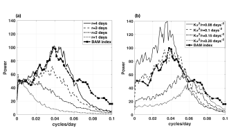
Figure 1: Power spectra of the stochastic oscillators represented by the equation (52) with several choices of the parameters $r$ and $K$ along with the power spectrum of the BAM index (Thompson and Woodworth, 2014). With the fixed $K=1/5\pi^{2}$, four different $r$’s are used for stochastic realization (a). Similarly, four different $K$’s are chosen for generating power spectra with a fixed $r=4$ (b).

Depending on the choice of the parameters $r$ and $K$, the equation (52) can show decayed oscillatory behavior or exponential decay. Under the assumption that $R_{1}/r+dR_{1}/d\tilde{t}$ is approximately a Gaussian white noise, we can simulate the equation to generate a stochastic realization. Figure 1 shows several power spectra of stochastic realizations from the equation (52) with different parameters $r$ and $K$ along with the power spectrum of the BAM index (Thompson and Woodworth, 2014). With a fixed $K$, four different memory time-scales from 1 day to 4 days are used for stochastic realization. In figure 1(a), we see that longer memory (4 days) leads to oscillatory behavior, which has the similar power spectrum with that of the BAM index, and shorter memory (1 day) to a red noise spectrum (Fig. 1a). Similarly, we fix $r=4$ days and vary $K$, which also shows the characteristics from stochastic oscillation to red noise process (Fig.1b). Similarly, when $K\pi^{2}/r=1\,\text{days}^{-2}$, the power spectrum is close to that of the BAM index.

The baroclinic wave life cycle results in recovering the vertical shear of the mean jet. This could be an origin of the finite memory effect in meridional heat transfer in planetary-scale, which leads to oscillatory behavior of zonal mean potential temperature. Following the above formalism, the fluctuation of potential temperature anomaly $\eta$ is represented as $\eta=\sum_{n=0}^{\infty}x_{n}(\tilde{t})Q_{n}(Y)$, hence $\partial\eta/\partial Y=\sum_{n=0}^{\infty}x_{n}(\tilde{t})dQ_{n}/dY$. By the thermal wind balance, $\partial U/\partial z\propto\sum_{n=0}^{\infty}x_{n}(\tilde{t})dQ_{n}/dY$, which implies that the vertical shear of the jet in lower levels could show quasi-oscillatory behavior depending on the time-scale of the eddy memory and relevant eigenvalues defining the decay time-scale of a specific normal mode.

The main focus lies on how to parameterize the meridional heat flux induced by synoptic eddies $\langle\overline{v_{0}\Theta_{0}}\rangle$ using the planetary-scale potential temperature $\Theta_{L}$. Considering that the time scale for synoptic eddies is not much smaller than that of planetary-scale motions, the meridional heat flux is not entirely determined by an instantaneous potential temperature gradient; instead it is dependent upon the temporal history of the potential temperature gradient. Hence, the Fickian diffusion approximation is not appropriate to parameterize the meridional heat flux induced by synoptic eddies. The simplest way considering the temporal history of the planetary-scale potential temperature is to introduce a time integration of the potential temperature with an appropriate memory kernel, which enables to include the past influence of planetary-scale mean fields on the turbulent heat flux. As a result, fluctuations of potential temperature can be described approximately by a generalized Langevin equation containing a memory term. The time-delayed effect represented as an integral kernel in the generalized Langevin equation can generate various types of variability ranging from simple red-noise process to quasi-oscillations and chaos. Hence, an appropriate choice of integral kernel is crucial to define the statistical characteristics of planetary-scale variability.

IV Conclusion

The main goal of the study was to rationalize the quasi-oscillatory variability of the BAM (Thompson and Barnes, 2014) on intra-seasonal time scales using the multi-scale representation of primitive equations of the large-scale atmosphere flow (Moon and Cho, 2020). Conceptually, the multi-scale approximation is a combination of the energy flux balance in the heat equation and the potential vorticity conservation. We found that the critical issue under the framework is the specification of an appropriate parameterization of the horizontal heat flux convergence from the synoptic and planetary-scale eddy dynamics. If the heat fluxes are represented using the simplest diffusive (Fickian) parameterization with a constant eddy diffusivity, the planetary-scale equations simplify to an energy flux balance with a meridional turbulent diffusion, similarly to North (1975). Other types of eddy parameterizations are also possible, of those most notable is the residual mean theory of Andrews and Mcintyre (1976) with a diffusive parameterization of isopycnal eddy fluxes of potential vorticity. While the residual mean formulation gives a different perspective on the mean flow dynamics compared to the direct diffusive closure of the heat fluxes (Schneider and Dickinson, 1974), our study questions their equilibrium-type Fickian assumption for the relation between the eddy fluxes and gradients of the considered tracer fields. Under the equilibrium-type eddy parameterizations, the main equation in the planetary-scales atmosphere is the heat equation with the basic balances resulting in a parabolic partial differential equation that does not support natural oscillations. The resulting temporal variability of observables obeys the Langevine equation leading to a red-noise spectrum that does not explain the quasi-oscillatory behavior of the BAM. Thus the equilibrium-type eddy parameterizations are likely not appropriate at the intraseasonal timescales and can only be used for representing the relatively long-term average of the planetary-scale dynamics.

We find that using a non-equilibrium eddy parameterization with the eddy memory effect represented by the delayed integral in the flux-gradient relation as was proposed for mesoscale ocean eddies (Manucharyan et al., 2017) can explain the oscillatory behavior of planetary-scale atmospheric flows. The rationalization for the eddy memory effect comes from the notion that the overall effect of synoptic eddies is to maintain the vertical shear of a mid-latitude jet (Robinson, 2000), implying that the eddy energy cycle starting from baroclinic instability near the surface could be considered as a finite timescale process. Thus, we hypothesized that the mid-latitude eddies have a finite memory and introduce a simple exponentially decaying memory kernel into the relation between the poleward eddy heat flux and the meridional potential temperature gradient. The inclusion of the finite memory kernel directly converts the heat equation from parabolic to wave equation that allows dispersive planetary-scale waves. As a result, instead of the red-noise model, the temporal variability of the anomalous potential temperature near the surface now obeys a stochastic oscillator model, with spectral characteristics that are similar to the observables associated with the BAM.

The key value of our theoretical study is that it highlights the processes and clarifies the physical interpretation of the crucial parameters that may be governing the spectral characteristics of the BAM. Specifically, our study implies that the period of natural oscillations of the BAM is proportional to the geometric mean between the eddy memory and the diffusive equilibration timescales. The ratio of these timescales controls the existence of a pronounced spectral peak while the variance is directly proportional to the external noise variance in the heat equation. Validating our key hypothesis about the exponential memory kernel and the finite eddy memory timescale in the relation between the mean flow and eddy heat fluxes using atmospheric models would be the next crucial step towards validating our theoretical arguments about the BAM. Furthermore, understanding the nature of the eddy memory and how its timescale depends on the mean flow or eddy characteristics would be necessary to understand the climate conditions under which the BAM could exhibit oscillatory behaviour. Finally, our results emphasize the importance of the external noise in driving the variance of the BAM and the necessity to understand if it is dependent on the mean flow or acts as an external/independent source of energy.