Estimation of the number of muons with muon counters

Abstract

The origin and nature of the cosmic rays is still uncertain. However, a big progress has been achieved in recent years due to the good quality data provided by current and recent cosmic-rays observatories. The cosmic ray flux decreases very fast with energy in such a way that for energies $\gtrsim 10^{15}$ eV, the study of these very energetic particles is performed by using ground based detectors. These detectors are able to detect the atmospheric air showers generated by the cosmic rays as a consequence of their interactions with the molecules of the Earth’s atmosphere. One of the most important observables that can help to understand the origin of the cosmic rays is the composition profile as a function of primary energy. Since the primary particle cannot be observed directly, its chemical composition has to be inferred from parameters of the showers that are very sensitive to the primary mass. The two parameters more sensitive to the composition of the primary are the atmospheric depth of the shower maximum and the muon content of the showers. Past and current cosmic-rays observatories have been using muon counters with the main purpose of measuring the muon content of the showers. Motivated by this fact, in this work we study in detail the estimation of the number of muons that hit a muon counter, which is limited by the number of segments of the counters and by the pile-up effect. We consider as study cases muon counters with segmentation corresponding to the underground muon detectors of the Pierre Auger Observatory that are currently taking data, and the one corresponding to the muon counters of the AGASA Observatory, which stopped taking data in 2004.

1 Introduction

The cosmic ray energy spectrum extends over several orders of magnitude in energy. The highest primary energies observed at present are of the order of $10^{20}$ eV. Above $\sim 10^{15}$ eV the cosmic ray flux is so small that these very energetic particles are studied by means of ground-based detectors, which are able to detect the atmospheric air showers generated by the cosmic ray interactions with the molecules of the atmosphere. Since the primary particle is not observed directly, its energy, arrival direction, and chemical composition have to be inferred from the shower information obtained by the detectors.

The origin of the cosmic rays is still unknown. The three main observables used to study their nature are: The energy spectrum, the distribution of their arrival directions, and the chemical composition. The composition of the primary particle has to be inferred from different properties of the showers. The most sensitive parameters to the primary mass are the atmospheric depth at which the shower reaches its maximum development and the muon content of the showers [1, 2, 3]. In general, the muon density at a given distance to the shower axis is used in composition analyses.

The composition profile as a function of energy is very important to understand several aspects of the cosmic-ray physics. In particular, at the highest energies the composition information plays an important role to find the transition between the galactic and extragalactic components of the cosmic rays [4, 5] and to elucidate the origin of the suppression observed at $\sim 10^{19.7}$ eV [6]. The composition analyses are subject to large systematic uncertainties originated by the lack of knowledge of the hadronic interactions at the highest energies (see for instance [7]). The composition is determined by comparing experimental data with simulations of the atmospheric showers and the detectors (when it corresponds). The showers are simulated by using high-energy hadronic interaction models that extrapolate low-energy accelerator data to the highest energies. This practice introduces large systematic uncertainties even when models updated using the Large Hadron Collider data are considered. Moreover, experimental evidence has been found recently about a muon deficit in shower simulations [8, 9]. Even though this is an important limitation for composition analyses, it is expected that mass-sensitive parameters, obtained with the next generation of high-energy hadronic interaction models, present smaller differences allowing for a reduction of the systematic uncertainties introduced by those models.

Past and current cosmic-rays experiments have been measuring muons by using different types of detectors [9]. A particular class of detector is the muon counter. This type of detectors has been used in the past in the Akeno Giant Air Shower Array (AGASA) [10] and at present in the Pierre Auger Observatory [11]. The muon counters are designed to count muons through a segmented detector. The segments of the Auger muon counters are scintillator bars whereas the segments of the AGASA muon counters were proportional counters. The limitation to measure a given number of incident muons is given by the number of segments of the counters.

In general, the principle of operation of the muon counters is based on a binary logic in which each channel of the electronics, associated to a given segment of the detector, is able to differentiate between a state in which the signal is larger than a given threshold level and the one in which it is smaller. The threshold level is chosen in such a way that almost all muons can be identified, i.e. the efficiency of each segment is close to $100\,\%$. For the case in which the signal is larger than the threshold level, the segment is said to be on and otherwise off. The time structure of the signal corresponding to one muon limits the time interval in which it is possible to identify single muons. This leads to the definition of a time interval, usually called inhibition window, in which it is decided whether a given segment is on or off. As a consequence, if one or more muons hit the same segment in a time interval of the order of the one corresponding to the inhibition window, the segment is tagged as on, losing the information about the number of muons that hit that segment. Therefore, when a given number of muons hit a muon counter in a time interval of the order of the one corresponding to the inhibition window, a number $k$ of segments on is obtained. If the number of incident muons is much smaller than the number of segments, the random variable $k$ is close the the number of muons that hit the counter. However, if the number of incident muons is close to the number of segments, the variable $k$ becomes much smaller than the number of incident muons. This effect is known as pile up [1].

In this work, we find an analytic expression for the distribution function of $k$, the number of segments on, given the number of incident muons, $n_{\mu}$. In this case, $k$ is the random variable and $n_{\mu}$ is taken as a parameter of the distribution. The expressions for the mean value and the variance of $k$ are inferred by using the new formula, these expressions are equal to the ones obtained in Ref. [1] by using a different approach. We also study how to estimate the parameter $n_{\mu}$ from measured values of $k$ and how to obtain a confidence interval. These studies are done for 192 segments, which correspond to the total number of segments of the Auger muon counters and 50 segments that correspond to the number of segments of muon counters used in AGASA.

It is worth mentioning that the main purpose of the muon counters is the reconstruction of the muon lateral distribution function (MLDF), i.e. the muon density as a function of the distance to the shower axis, which is proportional to the mean value of $n_{\mu}$. Even though the estimation of the mean value of $n_{\mu}$, which is studied in Ref. [12], is closely related to the determination of the MLDF, the estimation of $n_{\mu}$ is also important for different types of applications. In particular, it is important for the method used to reconstruct the MLDF developed in [1], in which an estimator of the number of muon that hit a given muon counter is inserted in the Poisson likelihood that approximates the exact likelihood in a given range of $n_{\mu}$. Also, the estimation of $n_{\mu}$ is necessary to obtain the calibration curve of the integrator (a complementary acquisition mode that muon counter can have), which is given by the mapping of the number of incident muons into the integrated signal [11]. The estimation of $n_{\mu}$ is also relevant for studies related to the signal fluctuations and systematic uncertainties performed by using twin muon counters [13].

2 Distribution function of the number of segments on and muon number estimation

The mean value of the number of muons, $n_{\mu}$, that hit a muon counter is given by,

$$\lambda=A\,\rho_{\mu}\,\cos\theta,$$ (1)

where $A$ is the area of the muon counters, $\rho_{\mu}$ is the muon density at a given distance to the shower axis, and $\theta$ is the zenith angle of the shower. Since the muon counters sample the MLDF at a given position in the shower plane, the number of muons that hit a given muon counter is a random variable that follows the Poisson distribution. The distribution of $k$ given $\lambda$ has been obtained in Ref. [12] and is given by

$$P(k|\,\lambda)={n_{s}\choose k}\,\exp(-\lambda)\left[\exp\left(-\lambda/n_{s}\right)-1\right]^{k},$$ (2)

where $n_{s}$ is the number of segments of the muon counter. Note that this distribution does not depend on the number of muons that hit the muon counters, which means that $P(k|\,\lambda)$ corresponds to the marginalization of the joint distribution $P(k,n_{\mu}|\,\lambda)$ with respect to $n_{\mu}$.

On the other hand, since all segments are equal, the probability distribution function corresponding to a given configuration of the number of muons that hit each segment in a time interval corresponding to one inhibition window is given by the multinomial distribution,

$$P(n_{1},\ldots,n_{n_{s}})=\frac{n_{\mu}!}{n_{1}!\ldots n_{n_{s}}!}\ \left(\frac{1}{n_{s}}\right)^{n_{\mu}},$$ (3)

where $n_{i}$ is the number of muons that hit the $i-$th segment. Here $\{n_{1},\ldots,n_{n_{s}}\}$ are such that $\sum_{i=1}^{n_{s}}n_{i}=n_{\mu}$.

The total number of segments on can be written in the following way,

$$k=\sum^{n_{s}}_{i=1}\widetilde{\Theta}(n_{i}),$$ (4)

where $\widetilde{\Theta}(n)=0$ if $n=0$ and $\widetilde{\Theta}(n)=1$ if $n\geq 1$. Note that $k\in\mathbb{N}$.

The mean value and the variance of $k$ can be calculated by using Eq. (3), as reported in Ref. [1]. The mean value and the variance of $k$ are given by (see A for details of the derivation),

$$\langle k\rangle(n_{\mu})\!\!\!\! = \!\!\!\!n_{s}\left[1-\left(1-\frac{1}{n_{s}}\right)^{n_{\mu}}\right],$$ (5)

$$\textrm{Var}\left[k\right](n_{\mu})\!\!\!\! = \!\!\!\!n_{s}\left(1-\frac{1}{n_{s}}\right)^{n_{\mu}}\left[1+(n_{s}-1)\left(1-\frac{1}{n_{s}-1}\right)^{n_{\mu}}\right.$$ (6)

$$-n_{s}\left.\left(1-\frac{1}{n_{s}}\right)^{n_{\mu}}\right].$$

Beyond the fact that the mean value and the variance of $k$ can be calculated from Eq. (3) in a relatively direct way, an analytic expression of the distribution function of $k$ given $n_{\mu}$, $P(k|\,n_{\mu})$, is more difficult to obtain. However, it can be inferred in a quite straightforward way by using the distribution $P(k|\,\lambda)$ given in Eq. (2). As mentioned before, $P(k|\,\lambda)$ is obtained marginalizing $P(k,n_{\mu}|\,\lambda)$ with respect to $n_{\mu}$. Besides, $P(k,n_{\mu}|\,\lambda)$ is given by the product of $P(k|\,n_{\mu})$ with the Poisson distribution. Therefore,

$$P(k|\,\lambda)\!\!\! = \!\!\!\sum_{n_{\mu}=\,0}^{\infty}P(k|\,n_{\mu})\,\exp(-\lambda)\,\frac{\lambda^{n_{\mu}}}{n_{\mu}!}$$ (7)

$$= \!\!\!{n_{s}\choose k}\,\exp(-\lambda)\left[\exp\left(-\lambda/n_{s}\right)-1\right]^{k}.$$

After introducing the following expression in Eq. (7),

$$\left[\exp\left(-\lambda/n_{s}\right)-1\right]^{k}\!\!\! = \!\!\!\sum_{j\,=\,0}^{k}{k\choose j}\,(-1)^{j}\exp\left(\lambda\,(k-j)/n_{s}\right),$$

$$\exp\left(\lambda\,(k-j)/n_{s}\right)\!\!\! = \!\!\!\sum_{n_{\mu}=\,0}^{\infty}\frac{\lambda^{n_{\mu}}}{n_{\mu}!}\left(\frac{k-j}{n_{s}}\right)^{n_{\mu}},$$ (8)

the form of $P(k|\,n_{\mu})$ is obtained comparing the terms proportional to $\lambda^{n_{\mu}}/n_{\mu}!$ in both sides of Eq. (2),

$$P(k|\,n_{\mu})={n_{s}\choose k}\,S(n_{\mu},k)\frac{k!}{n_{s}^{n_{\mu}}}.$$ (9)

Here $S(n_{\mu},k)$ is the Stirling number of second kind, which is given by

$$S(n_{\mu},k)=\frac{1}{k!}\,\sum_{j\,=\,0}^{k}{k\choose j}\,(-1)^{j}\,\left(k-j\right)^{n_{\mu}}.$$ (10)

The random variable $k$ ranges from $1$ to $n_{s}$. In the case in which $n_{\mu}<n_{s}$ and $k>n_{\mu}$, the condition $P(k|\,n_{\mu})=0$ must be fulfilled. To see this, it is enough to prove that $S(n_{\mu},k)=0$ when $n_{\mu}<n_{s}$ and $k>n_{\mu}$. For that purpose, let us consider the following expression of the Stirling number of second kind,

$$S(n_{\mu},k)=\frac{(-1)^{k}}{k!}\,\sum_{i\,=\,0}^{k}{k\choose i}\,(-1)^{i}\,i^{n_{\mu}}.$$ (11)

From this expression, it is easy to see that,

$$S(n_{\mu},k)=\left.\hat{\mathcal{O}}^{(n_{\mu})}f_{k}(x)\right|_{x=1},$$ (12)

where $\hat{\mathcal{O}}^{(n_{\mu})}$ corresponds to the differential operator $\hat{\mathcal{O}}=x\,d/dx$ applied $n_{\mu}$ times to the function $f_{k}(x)=(1-x)^{k}$. By using the definitions given above, the following expression is obtained,

$$\hat{\mathcal{O}}^{(n_{\mu})}f_{k}(x)=\sum_{i=1}^{n_{\mu}}a_{i}\,x^{i}\,\frac{d^{i}f_{k}}{dx^{i}}(x),$$ (13)

where $a_{i}$ are constant numbers. If $k>n_{\mu}$, all derivatives in Eq. (13) are proportional to a non-null and positive power of $(1-x)$. Therefore, it follows that $\hat{\mathcal{O}}^{(n_{\mu})}f_{k}(x)|_{x=1}=0$, which proves that $S(n_{\mu},k)=0$ for $k>n_{\mu}$ and then $P(k|\,n_{\mu})=0$ for $k>n_{\mu}$.

Since $P(k|\,n_{\mu})$ is a distribution function, it has to be normalized. To see that this is true for the expression in Eq. (9), let us consider the following property of the Stirling numbers of second kind [14],

$$x^{n_{\mu}}=\sum_{k=1}^{n_{\mu}}S(n_{\mu},k)\,(x)_{k},$$ (14)

where $(x)_{k}=x(x-1)...(x-k+1)$ is the falling factorial. If $x=n_{s}$, Eq. (14) becomes,

$$n_{s}^{n_{\mu}}=\left\{\begin{array}[]{ll}{\mathop{\displaystyle\sum_{k=1}^{n_{\mu}}}}S(n_{\mu},k)\,(n_{s})_{k}&n_{\mu}\leq n_{s}\\[11.38092pt] {\mathop{\displaystyle\sum_{k=1}^{n_{s}}}}S(n_{\mu},k)\,(n_{s})_{k}+{\mathop{\displaystyle\sum_{k=n_{s}+1}^{n_{\mu}}}}S(n_{\mu},k)\,(n_{s})_{k}&n_{\mu}>n_{s}\end{array}\right..$$ (15)

Using that $S(n_{\mu},k)=0$ for $k>n_{\mu}$ and that $(n_{s})_{k}=0$ for $k>n_{s}$, Eq. (15) can be written as

$$n_{s}^{n_{\mu}}=\sum_{k=1}^{n_{s}}{n_{s}\choose k}\,S(n_{\mu},k)\,k!,$$ (16)

which implies that

$$\sum_{k=1}^{n_{s}}P(k|\,n_{\mu})=\sum_{k=1}^{n_{s}}{n_{s}\choose k}\,S(n_{\mu},k)\,\frac{k!}{n_{s}^{n_{\mu}}}=1.$$ (17)

It is worth mentioning that from Eq. (9) it is possible to calculate the mean value and the variance of $k$ which have to be equal to the expressions obtained by using the multinomial distribution (see Eqs. (5) and (6)). The mean value of $k$ is given by

$$\langle k\rangle=\sum_{k=1}^{n_{s}}{n_{s}\choose k}\,S(n_{\mu},k)\,k\,\frac{k!}{n_{s}^{n_{\mu}}}.$$ (18)

From the recurrence satisfied by the Stirling numbers of second kind, $S(n_{\mu},k)=k\,S(n_{\mu}-1,k)+S(n_{\mu}-1,k-1)$ [14], it follows that $k\,S(n_{\mu},k)=S(n_{\mu}+1,k)+S(n_{\mu},k-1)$. Introducing this equality in Eq. (18), the following expression is obtained,

$$\langle k\rangle=\sum_{k=1}^{n_{s}}{n_{s}\choose k}\,S(n_{\mu}+1,k)\,\frac{k!}{n_{s}^{n_{\mu}}}-n_{s}\sum_{j=1}^{n_{s}-1}{n_{s}-1\choose j}\,S(n_{\mu},j)\,\frac{j!}{n_{s}^{n_{\mu}}},$$ (19)

where the second term of this equation is obtained by doing the change of variable $j=k-1$. From Eq. (16), it is easy to see that $\langle k\rangle=n_{s}^{n_{\mu}+1}/n_{s}^{n_{\mu}}-n_{s}\,(n_{s}-1)^{n_{\mu}}/n_{s}^{n_{\mu}}$, which after some algebra becomes $\langle k\rangle=n_{s}\,(1-(1-1/n_{s})^{n_{\mu}})$, i.e. the same expression obtained by using the multinomial distribution. In a similar way, but in this case using the recurrence relation satisfied by the Stirling number of second kind twice, it is possible to calculate the variance of $k$, whose expression obtained in this way is the same as the one obtained by using the multinomial distribution.

The Auger muon counters installed in each position of the array are composed of three modules of 64 segments each summing a total of 192 segments (see Ref. [11] for details). Figure 1 shows $P(k|\,n_{\mu})$ as a function of $k$ for different values of $n_{\mu}$. As expected, the maximum of the distribution is shifted towards larger values of $k$ for increasing values of $n_{\mu}$. Note that even for $n_{\mu}=1000$ the distribution $P(k|\,n_{\mu})$ presents a maximum.

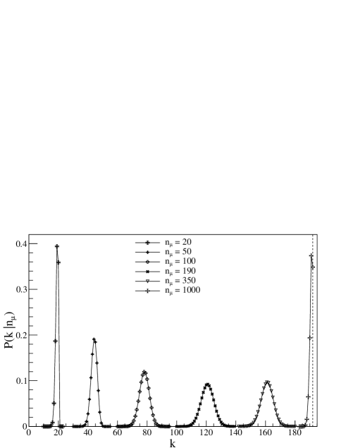
Figure 1: $P(k|\,n_{\mu})$ as a function of $k$ for $n_{s}=192$. The vertical dashed line corresponds to $k=192$. The solid lines joining the discrete points are added to guide the eye.

As a result of a measurement, a given value of $k$ is obtained. From this value of $k$ it is possible to estimate the parameter $n_{\mu}$ and to determine a confidence interval at a given confidence level. The maximum likelihood estimator of $n_{\mu}$, $\hat{n}_{\mu}$, is obtained by finding the maximum of the likelihood function $L(n_{\mu})=P(k|\,n_{\mu})$, i.e.,

$$\hat{n}_{\mu}=\underset{n_{\mu}\in\mathbb{N}}{\arg\max}\,P(k|\,n_{\mu}).$$ (20)

In this case, $\hat{n}_{\mu}$ has to be calculated numerically for each particular value of $k$ measured. Figure 2 shows the likelihood function as a function of $n_{\mu}$ for $k=100$ and $k=192$. From the top panel of the figure, it can be seen that for $k=100$ the likelihood presents a well-defined maximum as for all other allowed values of $k$ except for $k=192$. In this case, as can be seen from the bottom panel of the figure, the likelihood reaches a maximum for $n_{\mu}\rightarrow\infty$. This means that when the value $k=192$ is obtained as a result of a measurement, only a lower limit of $n_{\mu}$ can be found, as shown below. Note that $P(k=n_{s}|\,n_{\mu})\rightarrow 1$ when $n_{\mu}\rightarrow\infty$.

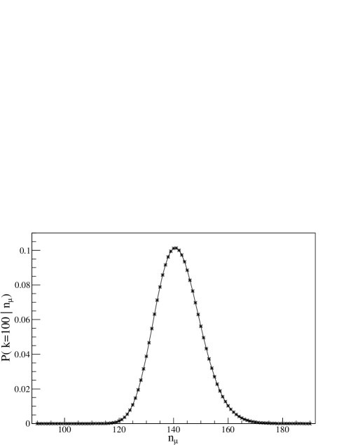
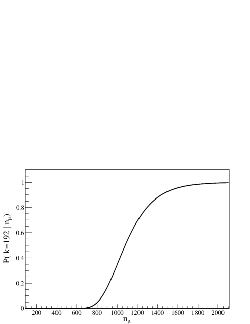
Figure 2: Likelihood function $L(n_{\mu})=P(k|\,n_{\mu})$ as a function of $n_{\mu}$ for $n_{s}=192$ and for $k=100$ (top panel) and $k=192$ (bottom panel). The solid lines joining the discrete points are added to guide the eye.

Figure 3 shows $\hat{n}_{\mu}$ as a function of $k$ obtained by maximizing the likelihood function for $n_{s}=192$. From the plot, it can be seen that $\hat{n}_{\mu}\cong k$ for small values of $k$. Moreover, $\hat{n}_{\mu}$ starts to deviate from $k$ in more than $10\,\%$ at $k\cong 40$. For larger values of $k$, $\hat{n}_{\mu}$ starts to increase faster in such a way that $\hat{n}_{\mu}=1007$ for $k=191$.

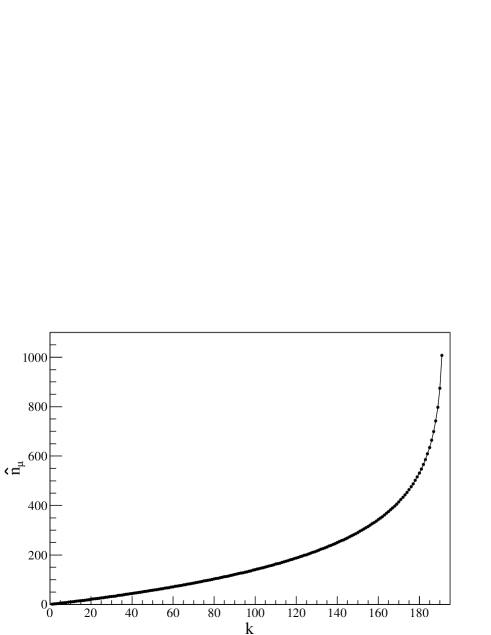
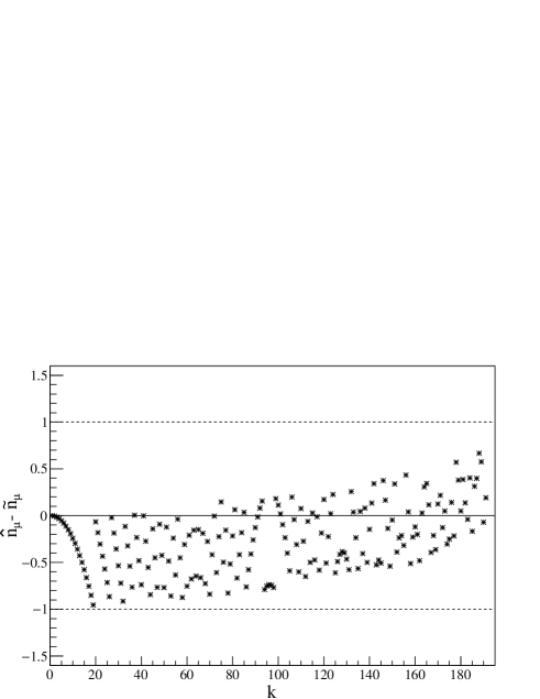
Figure 3: Top panel: Maximum likelihood estimator of $n_{\mu}$, $\hat{n}_{\mu}$, as a function of $k$. The solid line joining the discrete points is added to guide the eye. Bottom panel: Difference between $\hat{n}_{\mu}$ and $\widetilde{n}_{\mu}$ (approximated expression of $\hat{n}_{\mu}$ given by Eq. (21)) as a function of $k$. The number of segments considered is $n_{s}=192$.

As proposed in Ref. [1], a good approximation of $\hat{n}_{\mu}$ can be found by using the expression corresponding to the mean value of $k$ given in Eq. (5). Inverting Eq. (5), the expression

$$\widetilde{n}_{\mu}=\frac{\ln\left(1-{\mathop{\displaystyle\frac{k}{n_{s}}}}\right)}{\ln\left(1-{\mathop{\displaystyle{\frac{1}{n_{s}}}}}\right)},$$ (21)

is obtained, where the mean value of $k$ is replaced by the random variable $k$. The bottom panel of Fig. 3 shows the difference between the maximum likelihood estimator of $n_{\mu}$, $\hat{n}_{\mu}$, and the approximated expression of Eq. (21). It can be seen that $\widetilde{n}_{\mu}$ differs in less than one from $\hat{n}_{\mu}$ in the whole range of the variable $k$, which shows that $\widetilde{n}_{\mu}$ is a very good approximation of $\hat{n}_{\mu}$.

The confidence belt of the distribution function $P(k|\,n_{\mu})$ is constructed by finding the values of $k$, for a given $n_{\mu}$, that satisfy

$$\sum_{k}P(k|\,n_{\mu})\geq 1-\alpha,$$ (22)

where $1-\alpha$ is the confidence level (CL). In this work, the ordering proposed by Feldman and Cousins [15] is considered for the calculation of the confidence belt. The top panel of Fig. 4 shows the confidence belt of $P(k|\,n_{\mu})$ for $n_{s}=192$ and $1-\alpha=0.6827$. The $\hat{n}_{\mu}$ as a function of $k$ is also shown. From the figure it can be seen that the width of the confidence belt increases with $k$, as expected. It can also be seen that for $k=n_{s}=192$ only a lower limit can be obtained since the case $k=n_{s}$, i.e., all segments of the counter on is compatible with a semi-infinite set of $n_{\mu}$ values at any confidence level.

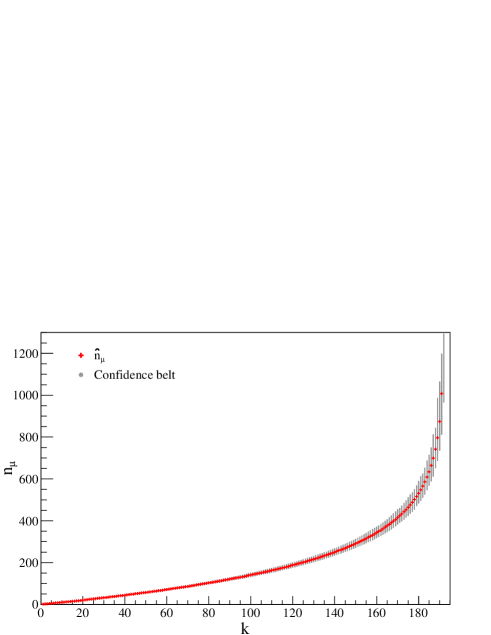
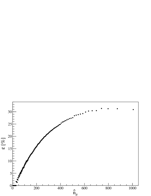
Figure 4: Top panel: Confidence belt of $P(k|\,n_{\mu})$ and $\hat{n}_{\mu}$ as a function of $k$. Bottom panel: $\varepsilon$ as a function of $\hat{n}_{\mu}$. The number of segments considered is $n_{s}=192$ and the confidence level used in the calculation is $1-\alpha=0.6827$.

The relative uncertainty of $\hat{n}_{\mu}$ is defined here as

$$\varepsilon=\frac{n_{\mu}^{max}-n_{\mu}^{min}}{2\,\hat{n}_{\mu}},$$ (23)

where $n_{\mu}^{max}$ and $n_{\mu}^{min}$ are the maximum and the minimum values of $n_{\mu}$, respectively, for a given value of $k$ obtained at a given CL. The bottom panel of Fig. 4 shows $\varepsilon$ as a function of $\hat{n}_{\mu}$. As expected, $\varepsilon$ increases with $\hat{n}_{\mu}$ taking values smaller than $\sim 16\,\%$ for $\hat{n}_{\mu}\lesssim 201$ and reaching values of the order of $30\,\%$ in the region where $700\lesssim\hat{n}_{\mu}\lesssim 900$ (close to $k=192$).

The determination of the mean value of the number of muons at a given distance to the shower axis $\lambda$, given by Eq. (1), is affected by the segmentation of the detector in combination with the pile-up effect and also by the Poisson fluctuations. Figure 5 shows the relative uncertainty corresponding to the estimator of the mean value of the Poisson distribution as a function of $n$, a measured valued of a Poisson random variable, which in this case coincides with the maximum likelihood estimator of the mean value. This relative uncertainty is obtained following the same procedure used to calculate the relative uncertainty corresponding to the $\hat{n}_{\mu}$ estimator. Comparing the bottom panel of Fig. 4 with Fig. 5 it can be seen that for values of $\hat{n}_{\mu}$ smaller than $\sim 113$ the uncertainty on the determination of the mean value of the number of muons is dominated by the Poisson fluctuations but for values of $\hat{n}_{\mu}$ larger than $\sim 113$ the dominant uncertainty is the one introduced by the segmentation of the detector in combination with the pile-up effect.

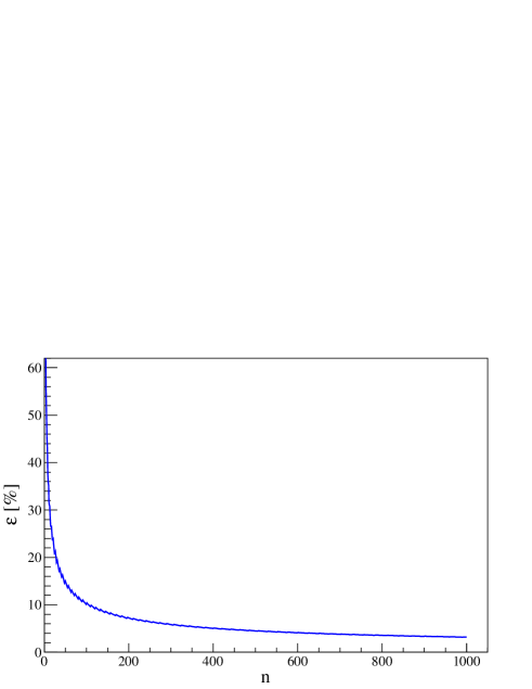
Figure 5: Relative uncertainty corresponding to the maximum likelihood estimator of the mean value of the Poisson distribution as a function of $n$, a measured value of a Poisson random variable. The confidence level used in the calculation is $1-\alpha=0.6827$.

The AGASA experiment used muon counters of 50 segments to measure the muon content of the showers. Figure 6 shows the distribution function $P(k|\,n_{\mu})$ as a function of $k$ for different values of $n_{\mu}$ and for $n_{s}=50$. As expected, for $n_{\mu}=250$ the maximum of the distribution is reached at $k=50$, which means that these counters saturate with a much smaller number of incident muons compared to the ones with 192 segments.

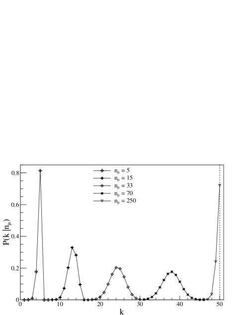
Figure 6: $P(k|\,n_{\mu})$ as a function of $k$ for $n_{s}=50$. The vertical dashed line corresponds to $k=50$. The solid lines joining the discrete points are added to guide the eye.

The top panel of Fig. 7 shows the maximum likelihood estimator of $n_{\mu}$ calculated numerically by using Eq. (20) for $n_{s}=50$. As for the $n_{s}=192$ case, $\hat{n}_{\mu}\cong k$ for small values of $k$ in such a way that for $k>20$, the departure of $\hat{n}_{\mu}$ from $\hat{n}_{\mu}\cong k$ becomes larger than $10\,\%$. For larger values of $k$, $\hat{n}_{\mu}$ starts to increase faster in such a way that $\hat{n}_{\mu}=194$ for $k=49$.

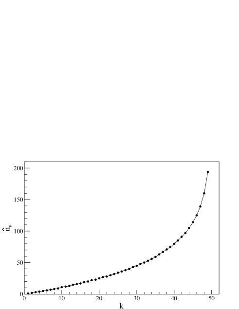
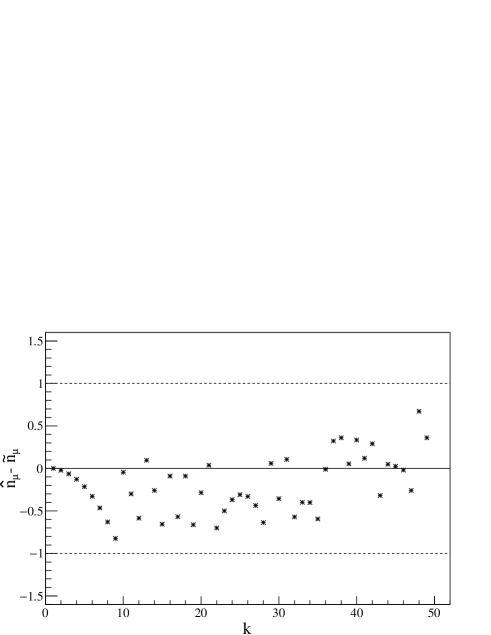
Figure 7: Top panel: Maximum likelihood estimator of $n_{\mu}$, $\hat{n}_{\mu}$, as a function of $k$. The solid line joining the discrete points is added to guide the eye. Bottom panel: Difference between $\hat{n}_{\mu}$ and $\widetilde{n}_{\mu}$ (approximated expression of $\hat{n}_{\mu}$ given in Eq. (21)) as a function of $k$. The number of segments considered is $n_{s}=50$.

The bottom panel of Fig. 7 shows $\hat{n}_{\mu}-\widetilde{n}_{\mu}$ as a function of $k$. Also in this case, the absolute value of this difference is smaller than one, which indicates that $\widetilde{n}_{\mu}$, given in Eq. (21), is a very good approximation of $\hat{n}_{\mu}$ also for the $n_{s}=50$ case.

The top panel of Fig. 8 shows the confidence belt of $P(k|\,n_{\mu})$ for $n_{s}=50$ and $1-\alpha=0.6827$. The $\hat{n}_{\mu}$ as a function of $k$ is also shown in the plot. As in the case corresponding to $n_{s}=192$, the confidence belt becomes wider for increasing values of $k$. This behavior becomes more evident from the plot in the bottom panel of the same figure, in which it can be seen that the relative uncertainty of $\hat{n}_{\mu}$ is smaller than $\sim 16\,\%$ for $k\leq 67$ and takes values close to $24\,\%$ in the region where $140\lesssim k\lesssim 194$.

Figure 8: Top panel: Confidence belt of $P(k|\,n_{\mu})$ and $\hat{n}_{\mu}$ as a function of $k$. Bottom panel: $\varepsilon$ as a function of $\hat{n}_{\mu}$. The number of segments considered is $n_{s}=50$ and the confidence level used in the calculation is $1-\alpha=0.6827$.

As in the previous case, comparing the bottom panel of Fig. 8 with Fig. 5 it can be seen that for values of $\hat{n}_{\mu}$ smaller than $\sim 55$ the uncertainty on the determination of the mean value of the number of muons is dominated by the Poisson fluctuations but for values of $\hat{n}_{\mu}$ larger than $\sim 55$ the dominant uncertainty is the one introduced by the segmentation of the detector in combination with the pile-up effect.

Note that the relative uncertainty on the determination of $\hat{n}_{\mu}$ for the AGASA muon counters cannot be compared straightforwardly with the one corresponding to Auger, since the area of the AGASA muon counters is 25 m² whereas the one corresponding to the Auger muon counters is 30 m². Therefore, the number of muons that hit an AGASA muon detector is, on average, $\sim 17\,\%$ smaller than the one corresponding to an Auger muon detector, provided that the muon flux that hit the detectors is the same. In any case, the determination of the muon density at a given distance to the shower axis done by using the Auger muon detectors should be better than the one corresponding to the AGASA muon detectors, since the Auger muon detectors have a larger area and a larger number of segments ($A=30$ m² and $n_{s}=192$) than the ones corresponding to AGASA ($A=25$ m² and $n_{s}=50$).

The estimation of the number of muons studied in this work corresponds to ideal muon detectors. Real detectors are subject to different effects that have to be taken into account in order not to introduce biases in the estimated number of muons. For instance, there are three main effects that can introduce biases in the Auger muon detectors. The first one is the noise produced by the dark rate of the silicon photomultipliers, which can reach the discriminator threshold due to the inner-cells crosstalk. This effect can be mostly reduced choosing a proper counting strategy (see Ref. [11] for details). The second one is the efficiency of each segment, which can be smaller than 100 %. In this case a correction can be obtained from the estimated efficiency, which is measured in the laboratory [11]. Note that the efficiency of the Auger muon detectors is $\sim 98.5$ %. The third one is caused by particles passing through two adjacent segments, the bias introduced by this effect can be estimated form detailed simulations of the detector [16]. Note that the sources of biases on the estimation of the number of incident muons depend on the specific design of the muon detector under consideration and have to be studied in detail for each particular case.

3 Conclusions

In this work we have studied in detail the estimation of the number of muons that hit a muon counter from the number of segments on, $k$, which is the random variable that is measured in an experiment. For that purpose we have found an analytic expression for the distribution function of $k$, given a number of incident muons. We have considered the number of segments corresponding to the muon counters of Auger and also the one corresponding to the muon counters of AGASA.

We have found that for small values of $k$, compared with the number of segments, the estimator of the muon number is close to $k$ but increases much faster for larger values of $k$. We have also found that the relative uncertainty in the determination of the number of muons is small for small values of $k$ and that it increases relatively fast with $k$ reaching values close to $24$ and $30\,\%$, for $n_{s}=50$ and $n_{s}=192$ respectively, in the region where $k$ is close to the total number of segments.

The main motivation of these studies is the measurement of the muon content of air showers initiated by cosmic rays, which is intimately related to the chemical composition of the primary particle, an open problem of the high-energy astrophysics. However, it is worth mentioning that the methods developed in this work can be relevant in other applications.

Appendix A Calculation of $\langle k\rangle$ and Var[$k$] from the multinomial distribution

In this section, the steps that lead to the expressions for $\langle k\rangle$ and Var[$k$] (see Eqs. (5) and (6)), obtained in Ref. [1] by using the multinomial distribution are given.

Let us start with the calculation of the mean value of $k$. From Eq. (4) it can be seen that,

$$\langle k\rangle=\left\langle\sum^{n_{s}}_{i=1}\widetilde{\Theta}(n_{i})\right\rangle=n_{s}\left\langle\widetilde{\Theta}(n_{1})\right\rangle.$$ (24)

The distribution function of $n_{1}$ is given by the binomial distribution, i.e.

$$P_{1}(n_{1})={n_{\mu}\choose n_{1}}\,\left(\frac{1}{n_{s}}\right)^{n_{1}}\,\left(1-\frac{1}{n_{s}}\right)^{n_{\mu}-n_{1}}.$$ (25)

Therefore,

$$\langle k\rangle=n_{s}\sum_{n_{1}=0}^{n_{\mu}}\widetilde{\Theta}(n_{1})\,P_{1}(n_{1})=n_{s}\sum_{n_{1}=1}^{n_{\mu}}P_{1}(n_{1})=n_{s}\,(1-P_{1}(0)).$$ (26)

Combining Eqs. (25) and (26), the expression for the mean value of $k$ given by Eq. (5) is obtained.

The variance of $k$ is calculated in a similar way. For that purpose, let us first calculate the mean value of $k^{2}$, which is given by

$$\langle k^{2}\rangle\!\!\! = \!\!\!\left\langle\sum^{n_{s}}_{i=1}\sum^{n_{s}}_{j=1}\widetilde{\Theta}(n_{i})\,\widetilde{\Theta}(n_{j})\right\rangle$$ (27)

$$= \!\!\!n_{s}\left\langle\widetilde{\Theta}^{2}(n_{1})\right\rangle+n_{s}(n_{s}-1)\left\langle\widetilde{\Theta}(n_{1})\,\widetilde{\Theta}(n_{2})\right\rangle.$$

To calculate the averages in Eq. (27) besides $P_{1}(n_{1})$, $P_{2}(n_{1},n_{2})$ is required. From Eq. (3) it can be seen that

$$P_{2}(n_{1},n_{2})=\frac{n_{\mu}!}{n_{1}!n_{2}!(n_{\mu}-n_{1}-n_{2})!}\left(\frac{1}{n_{s}}\right)^{n_{1}+n_{2}}\,\left(1-\frac{2}{n_{s}}\right)^{n_{\mu}-n_{1}-n_{2}},$$ (28)

where $n_{1}+n_{2}\leq n_{\mu}$. In a similar way to the one followed to obtain Eq. (26), the next expression for the mean value $k^{2}$ is obtained

$$\langle k^{2}\rangle\!\!\! = \!\!\!n_{s}\,(1-P_{1}(0))+n_{s}(n_{s}-1)\times$$ (29)

$$\!\!\!\left(1-P_{2}(0,0)-2\sum_{n_{1}=1}^{n_{\mu}}P_{2}(n_{1},0)\right).$$

By using that,

$$\sum_{n_{1}=1}^{n_{\mu}}P_{2}(n_{1},0)=\left(1-\frac{1}{n_{s}}\right)^{n_{\mu}}-\left(1-\frac{2}{n_{s}}\right)^{n_{\mu}},$$ (30)

the following expression is obtained,

$$\langle k^{2}\rangle=n_{s}^{2}-n_{s}(2n_{s}-1)\left(1-\frac{1}{n_{s}}\right)^{n_{\mu}}+n_{s}(n_{s}-1)\left(1-\frac{2}{n_{s}}\right)^{n_{\mu}}.$$ (31)

From Eqs. (31) and (5), the expression for the variance of $k$ given by Eq. (6) is obtained.

References

- [1] A.D. Supanitsky, et al., Underground muon counters as a tool for composition analyses, Astropart. Phys. 29 (2008) 461.
- [2] A.D. Supanitsky, G. Medina-Tanco, and A. Etchegoyen, On the possibility of primary identification of individual cosmic ray showers, Astropart. Phys. 31 (2009) 116.
- [3] K. Kampert and M. Unger, Measurements of the cosmic ray composition with air shower experiments, Astropart. Phys. 35 (2012) 660.
- [4] G. Medina-Tanco for The Pierre Auger Collaboration, Astrophysics Motivation behind the Pierre Auger Southern Observatory Enhancements, Proc. of ICRC, Merida, Mexico, 1101 (2007).
- [5] R. Aloisio, V. Berezinsky, and A. Gazizov, Transition from galactic to extragalactic cosmic rays, Astropart. Phys. 39-40 (2012) 129.
- [6] K. Kampert, Ultrahigh-Energy Cosmic Rays: Results and Prospects, Brazilian Journal of Physics, 43 (2013) 375.
- [7] A.D. Supanitsky, G. Medina-Tanco, and A. Etchegoyen, A new numerical technique to determine primary cosmic ray composition in the ankle region, Astropart. Phys. 31 (2009) 75.
- [8] F. Gesualdi, A.D. Supanitsky, and A. Etchegoyen, Muon deficit in air shower simulations estimated from AGASA muon measurements, Phys. Rev. D, 101 (2020) 083025.
- [9] L. Cazon for the EAS-MSU, IceCube, KASCADE-Grande, NEVOD-DECOR, Pierre Auger, SUGAR, Telescope Array, and Yakutsk EAS Array Collaborations, Working group report on the combined analysis of Muon Density Measurements from Eight Air Shower Experiments, Proc. of the ICRC, PoS(ICRC2019) (2019) 214.
- [10] N. Hayashida et al., Muons ( 1 GeV) in large extensive air showers of energies between eV and eV observed at Akeno, J. Phys. G 21 (1995) 1101.
- [11] A. Botti for the Pierre Auger Collaboration, The AMIGA underground muon detector of the Pierre Auger Observatory - performance and event reconstruction, Proc. of the ICRC, PoS(ICRC2019) (2019) 202.
- [12] D. Ravignani and A.D. Supanitsky, A new method for reconstructing the muon lateral distribution with an array of segmented counters, Astropart. Phys. 65 (2015) 1.
- [13] B. Wundheiler for the Pierre Auger Collaboration, The AMIGA Muon Counters of the Pierre Auger Observatory: Performance and Studies of the Lateral Distribution Function, Proc. of the ICRC, PoS(ICRC2015) (2015) 324.
- [14] R. Stanley, Enumerative Combinatorics, second ed., Cambridge University Press, New York, 2012.
- [15] G. Feldman and R. Cousins, Unified approach to the classical statistical analysis of small signals, Phys. Rev. D 57 (1998) 3873.
- [16] J. Figueira for the Pierre Auger Collaboration, An improved reconstruction method for the AMIGA detectors, Proc. of the ICRC, PoS(ICRC2017) (2017) 396.