On the interference of $ggH$ and ${c\bar{c}}H$ Higgs production mechanisms and the determination of charm Yukawa coupling at the LHC

Abstract

Higgs boson production in association with a charm-quark jet proceeds through two different mechanisms – one that involves the charm Yukawa coupling and the other that involves direct Higgs coupling to gluons. The interference of the two contributions requires a helicity flip and, therefore, cannot be computed with massless charm quarks. In this paper, we consider QCD corrections to the interference contribution starting from charm-gluon collisions with massive charm quarks and taking the massless limit, $m_{c}\to 0$. The behavior of QCD cross sections in that limit differs from expectations based on the canonical QCD factorization. This implies that QCD corrections to the interference term necessarily involve logarithms of the ratio $M_{H}/m_{c}$ whose resummation is currently unknown. Although the explicit next-to-leading order QCD computation does confirm the presence of up to two powers of $\ln(M_{H}/m_{c})$ in the interference contribution, their overall impact on the magnitude of QCD corrections to the interference turns out to be moderate due to a cancellation between double and single logarithmic terms.

1 Introduction

Studies of Yukawa couplings play an important role in the verification of the mechanism of electroweak symmetry breaking as described by the Standard Model. By now, Higgs couplings to bottom and top quarks, as well as to tau leptons and muons, have been measured to a precision of about twenty percent Aaboud:2018zhk ; Sirunyan:2018kst ; Aaboud:2018pen ; Sirunyan:2018cpi ; Aad:2020xfq ; Sirunyan:2018hbu . Within the error bars, the measured values for all four Yukawa couplings are consistent with the Standard Model predictions.

However, the Yukawa couplings to lighter fermions have not been studied experimentally. Although it is generally agreed that the Yukawa couplings of electrons and up, down and strange quarks can be observed if and only if they enormously deviate from their Standard Model values, the situation with the charm Yukawa is not so hopeless. In fact, it appears that with the full LHC luminosity, the charm Yukawa coupling can be measured if its value deviates from the Standard Model expectation by an order one factor Perez:2015lra . Different observables to measure the charm Yukawa coupling at the LHC have been proposed; they include inclusive ($H\to c\bar{c}$) and exclusive ($H\to J/\psi+\gamma$ and similar) decays of the Higgs boson kagan ; Modak:2014ywa ; Koenig:2015pha , the modifications of the Higgs transverse momentum distribution Bishara:2016jga in the $gg\to H+X$ process and, finally, Higgs boson production cross section in association with a charm jet Brivio:2015fxa .

In this paper we focus on the latter process, $pp\to H+{\rm jet}_{c}$. At leading order in perturbative QCD, Higgs bosons are produced in association with charm jets in the partonic process $cg\to Hc$. The amplitude of this process receives contributions proportional to the charm Yukawa coupling and to an effective $ggH$ coupling

$${\cal M}\sim g_{{\rm Yuk}}{\cal M}_{1}+g_{ggH}{\cal M}_{2},$$ (1)

see Figure 1. As a result, the $pp\to H+{\rm jet}_{c}$ cross section contains the interference term

$$\sigma_{Hc}\sim g_{{\rm Yuk}}^{2}\;\tilde{\sigma}_{1}+g_{ggH}^{2}\;\tilde{\sigma}_{2}+g_{{\rm Yuk}}g_{ggH}\;\tilde{\sigma}_{{\rm Int}}.$$ (2)

It can be expected that a reliable description of Higgs boson production in association with a charm jet can be obtained by systematically computing the different terms in Eq. (2) to higher orders in perturbative QCD. In fact, it is emphasized in Ref. Brivio:2015fxa that the largest theoretical uncertainty in using $H+{\rm jet}_{c}$ production cross section to constrain charm Yukawa coupling is related to perturbative QCD uncertainties so that it seems natural to compute higher order QCD corrections to $\sigma_{Hc}$ in Eq. (2).

However, pursuing this program for the interference term in Eq. (2) is quite subtle as we now discuss. Indeed, perturbative computations in QCD are performed with massless incoming partons. In case of the massless charm quark that, however, has non-vanishing Yukawa coupling to the Higgs boson, the interference term in Eq. (2) vanishes and we obtain

$$\lim_{m_{c}\to 0}\sigma_{Hc}\sim g_{{\rm Yuk}}^{2}\tilde{\sigma}_{1}+g_{ggH}^{2}\tilde{\sigma}_{2}.$$ (3)

This happens because the Yukawa interaction flips charm’s helicity but the gluon-charm interaction conserves it; hence, the two contributions in Eq. (1) cannot interfere if $m_{c}=0$. For the massive charm quark the interference does not vanish and is proportional to the charm mass in the first power. Whether or not the interference contribution is negligible depends on the relative magnitude of the two amplitudes in Eq. (1). Leading-order computations with massless quarks show that the charm-Yukawa independent amplitude $g_{ggH}{\cal M}_{2}$ in Eq. (1) is larger than the charm-Yukawa dependent one $g_{{\rm Yuk}}{\cal M}_{1}$ suggesting that the interference may be non-negligible.

It is straightforward to calculate the interference at leading order in perturbative QCD. Indeed, the interference requires one helicity flip on a charm line that connects initial and final states; this flip is accomplished by a single mass insertion. This implies that one can compute the interference of the two amplitudes using massive charm quarks, take the $m_{c}\to 0$ limit and account for the first non-vanishing term proportional to $m_{c}$. Since we require a charm jet in the final state, none of the kinematic invariants of the $cg\to Hc$ process can be small. Hence, once one power of $m_{c}$ is extracted, the rest of the leading-order calculation of the interference contribution can be performed using the standard approximation of massless (charm) quarks. Such calculation, that we describe in Section 5, shows that the leading-order interference amounts to about ten percent of the contribution to the $H+{\rm jet}_{c}$ cross section that is proportional to the Yukawa coupling squared.

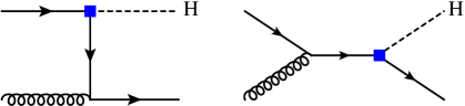
(a) Yukawa coupling

(b) Effective ${ggH}$ vertex

Figure 1: Leading-order Feynman diagrams contributing to the $pp\to Hc$ process. We distinguish two separate production mechanisms: one that is driven by the Yukawa coupling (left) and the other one that requires direct coupling of Higgs to gluons (right).

Although the interference contribution is not large, it is worth thinking about it at next-to-leading order (NLO) in perturbative QCD since there are reasons to believe that the interference contribution is perturbatively unstable, at variance with the two other contributions to $pp\to H+{\rm jet}_{c}$ cross section. Indeed, even if we require an energetic charm jet in the final state, soft and collinear kinematic configurations lead to logarithmic sensitivity of the interference to the charm mass $m_{c}$. Hence, before the $m_{c}\to 0$ approximation can be taken, the quasi-singular contributions proportional to logarithms of $m_{c}$ have to be extracted from both real and virtual corrections to the interference part of the production cross section.

One may argue that, since the finite charm mass provides yet another way to regulate collinear divergences, it is to be expected that the procedure described above will lead to a familiar picture of (quasi)-collinear factorization of QCD amplitudes. If so, all $\ln(m_{c})$–dependent terms should disappear once infrared safe cross sections and distributions are computed using short-distance quantities, including conventional parton distribution functions (PDFs). However, we will show that for the interference contribution this expectation is invalid and that well-known formulas that describe collinear factorization of mass singularities are not applicable in that case. We will also show that the helicity flip leads to an appearance of soft-quark singularities that, interestingly, make jet algorithms logarithmically-sensitive to $m_{c}$.

There are two consequences of the above discussion. First, the problem of estimating the magnitude of the interference contribution to the production of a Higgs boson in association with a charm jet turns into an interesting problem in perturbative QCD that borders on such important issues as soft and collinear QCD factorization for mass power corrections Penin:2014msa ; Melnikov:2016emg ; Liu:2019oav ; Liu:2020wbn ; Laenen:2020nrt . Second, a more complex pattern of this factorization, as compared to the canonical collinear and soft cases Catani:2000ef , implies that NLO QCD corrections to leading-order interference are enhanced by up to two powers of a large logarithm $\ln Q/m_{c}$ where $Q$ is a typical hard scale in the process $pp\to H+{\rm jet}_{c}$. For this reason NLO QCD corrections to the interference may be expected to be significant and it becomes essential to explicitly compute them. This is what we set out to do in this paper.

The rest of the paper is organized as follows. In the next section we derive a relation between ${\overline{\rm MS}}$-regulated and mass-regulated parton distribution functions at ${\cal O}(\alpha_{s})$ using the process of Higgs boson production in $c\bar{c}$ annihilation. We use the established relation to remove “conventional” collinear logarithms from NLO QCD corrections to the interference contribution to the production of Higgs boson in association with charm jet. In Section 3 we discuss factorization of mass singularities in the interference contribution to $cg\to Hc$ process and show that it works differently as compared to the standard case Catani:2000ef . In Section 4 we briefly describe the technical details of the calculation of NLO QCD corrections to the interference contribution. In Section 5 we present phenomenological results and discuss the relative importance of logarithmically-enhanced terms. We conclude in Section 6. Additional discussion of soft and collinear limits of the interference contributions as well as some relevant soft integrals can be found in several appendices.

2 Matching parton distribution functions

It is well-known that quark masses screen collinear singularities. For this reason we can think about small quark masses as a particular choice of a collinear regulator. Since, when describing “leading-twist” inclusive partonic processes, collinear sensitivity either cancels out or is absorbed into parton distribution functions, it is possible to derive relations between parton distribution functions that are used for computations with nearly massive and strictly massless quarks by requiring that predictions for physical processes are independent of a collinear regulator.

To derive a relation between “massive” and “massless” PDFs, we start with the production of a Higgs boson in an annihilation of two massive charm quarks and write the differential cross section as

$${\rm d}\sigma_{pp\to H}=\sum\limits_{ij}\;\int{\rm d}x_{1}\,{\rm d}x_{2}\,f^{(m)}_{i}(x_{1})f^{(m)}_{j}(x_{2}){\rm d}\hat{\sigma}^{(m)}_{ij\to H+X}.$$ (4)

Here $f_{i}^{(m)}$ are parton distribution functions and the superscript $m$ implies that all relevant quantities should be computed using quark masses as collinear regulators. Also, $\hat{\sigma}^{(m)}_{ij\to H+X}$ is the partonic differential cross-section. At leading order $i(j)=c,\bar{c}$; at higher orders other channels also contribute.

Calculation at leading order in $\alpha_{s}$ is straightforward since the leading-order cross section $\sigma^{(m)}_{c\bar{c}\to H}$ has a regular $m_{c}\to 0$ limit. It follows that at leading order in $\alpha_{s}$ there is no difference between $f_{i}^{(m)}$ and conventional ${\overline{\rm MS}}$ parton distribution functions, i.e. $f^{(m)}_{i}=f^{\overline{\rm MS}}_{i}$.

The situation becomes more complicated at next-to-leading order where the charm quark mass screens collinear singularities; hence, our goal is to re-write the NLO QCD contributions to the cross section $c\bar{c}\to H+X$ in such a way that logarithms of $m_{c}$ are extracted explicitly.

We begin by considering the process $c(p_{1})+\bar{c}(p_{2})\to H+g(p_{3})$ and treating charm quarks as massive. Kinematic regions that lead to soft and (quasi-)collinear singularities are well understood. The behavior of matrix elements in these limits is described by conventional factorization formulas Catani:2000ef . We can define a hard $m_{c}$-independent cross section by subtracting the singular limits. When the subtracted terms are added back and integrated over unresolved parts of the $Hg$ phase space, logarithms of the charm mass appear. This procedure is identical to methods developed to extract infrared and collinear singularities from real emission contributions to partonic cross sections. Its application in the present context allows us to explicitly extract logarithms of the charm mass.

To organize the calculation, we follow the nested soft-collinear subtraction scheme Caola:2017dug ; Caola:2019nzf ; Caola:2019pfz ; Asteriadis:2019dte which, at next-to-leading order, is equivalent to the FKS scheme Frixione:1995ms ; Frixione:1997np . We use dimensional regularization to regularize soft singularities and the charm mass to regularize the collinear ones. Using notations from Ref. Caola:2017dug , we write the partonic cross section for $c(p_{1})+\bar{c}(p_{2})\to H+g(p_{3})$ as

$$\begin{split}&2s\cdot{\rm d}\hat{\sigma}_{c\bar{c}\to H+g}=\int[{\rm d}g_{3}]F_{\rm LM}(1_{c},2_{\bar{c}};3_{g})\equiv\langle F_{\rm LM}(1_{c},2_{\bar{c}};3_{g})\rangle=\langle S_{3}F_{\rm LM}(1_{c},2_{\bar{c}};3_{g})\rangle\\ &+\langle(C_{31}+C_{32})(I-S_{3})F_{\rm LM}(1_{c},2_{\bar{c}};3_{g})\rangle+\langle(I-C_{31}-C_{32})(I-S_{3})F_{\rm LM}(1_{c},2_{\bar{c}};3_{g})\rangle.\end{split}$$ (5)

The key observation is that since the fully-regulated (last) term in Eq. (5) is free of both soft and quasi-collinear singularities, the limit $m_{c}\to 0$ can be safely taken there. On the contrary, both soft and collinear subtraction terms exhibit mass singularities; these mass singularities need to be extracted.

Consider the soft limit defined as ${p_{3}\!\cdot\!p_{1}}\sim{p_{3}\!\cdot\!p_{2}}\to 0$. It reads Catani:2000ef

$$S_{3}F_{\rm LM}(1_{c},2_{\bar{c}};3_{g})\approx g_{s}^{2}C_{F}\left(\frac{2(p_{1}\cdot p_{2})}{(p_{1}\cdot p_{3})(p_{2}\cdot p_{3})}-\frac{m_{c}^{2}}{(p_{1}\cdot p_{3})^{2}}-\frac{m_{c}^{2}}{(p_{2}\cdot p_{3})^{2}}\right)F_{\rm LM}(1_{c},2_{\bar{c}}),$$ (6)

where $g_{s}$ is the unrenormalized strong coupling constant.

Since the soft gluon decouples from the function $F_{\rm LM}(1_{c},2_{\bar{c}})$ we can integrate Eq. (6) over the gluon phase space. We work in the center-of-mass frame of the colliding charm partons and parametrize their energies as $E_{1}=E_{2}=E$. The center of mass energy squared in the massless approximation is then $s=4E^{2}$. We also cut integrals over gluon energy at $E_{3}=E_{\rm max}$, cf. Ref Caola:2017dug . Integrating Eq. (6) over gluon phase space $[{\rm d}g_{3}]$ and taking the $m_{c}\to 0$ limit, we find

$$\langle S_{3}F_{\rm LM}(1_{c},2_{c};3_{g})\rangle=-\frac{C_{F}\left[\alpha_{s}\right]E_{\rm max}^{-2\epsilon}}{\epsilon}\big{[}2\;I_{1m}(E)-I_{2m}(E)\big{]}\langle F_{\rm LM}({\tilde{1}_{c}},\tilde{2}_{\bar{c}})\rangle,$$ (7)

where $[\alpha_{s}]=g_{s}^{2}\Omega^{(d-2)}/(2(2\pi)^{d-1})$ and $\Omega^{(d-2)}$ is the solid angle of the $(d-2)$-dimensional space. The notation $\tilde{1}_{c}(\tilde{2}_{\bar{c}})$ implies that the corresponding four-momenta should be taken in the massless approximation. The two integrals $I_{1m(2m)}$ in Eq. (7) read

$$\begin{split}&I_{1m}(E)=\int\limits_{-1}^{1}\frac{{\rm d}\cos\theta(\sin^{2}\theta)^{-\epsilon}}{1-\beta\cos\theta}\approx-\frac{4^{-\epsilon}\Gamma^{2}(1-\epsilon)}{\epsilon\;\Gamma(1-2\epsilon)}\left[1-\frac{\Gamma(1+\epsilon)\Gamma(1-2\epsilon)}{\Gamma(1-\epsilon)}\left(\frac{m_{c}^{2}}{4E^{2}}\right)^{-\epsilon}\right],\\ &I_{2m}(E)=\frac{m_{c}^{2}}{E^{2}}\int\limits_{-1}^{1}\frac{{\rm d}\cos\theta(\sin^{2}\theta)^{-\epsilon}}{\left(1-\beta\cos\theta\right)^{2}}\approx 2\left(\frac{m_{c}^{2}}{E^{2}}\right)^{-\epsilon}\Gamma(1-\epsilon)\Gamma(1+\epsilon),\end{split}$$ (8)

where $\beta=\sqrt{1-m_{c}^{2}/E^{2}}$ and we neglected all power-suppressed terms when writing the results.

Collinear subtraction terms contain quasi-collinear singularities. The two collinear limits correspond to two distinct cases, ${p_{1}\!\cdot\!p_{3}}\sim m_{c}^{2}\to 0$ and ${p_{2}\!\cdot\!p_{3}}\sim m_{c}^{2}\to 0$. They read

$$C_{3i}\;F_{\rm LM}(1_{c},2_{\bar{c}};3_{g})=\frac{g_{s}^{2}}{(p_{i}\cdot p_{3})}\left[P_{qq}(z)-\frac{C_{F}m_{c}^{2}z}{(p_{i}\cdot p_{3})}\right]\frac{F^{(i)}_{\rm LM}({\tilde{1}_{c}},\tilde{2}_{\bar{c}};z)}{z},$$ (9)

where

$$F^{(i)}_{\rm LM}({\tilde{1}_{c}},\tilde{2}_{\bar{c}};z)=\delta_{i1}\;F_{\rm LM}(z\cdot{\tilde{1}_{c}},\tilde{2}_{\bar{c}})+\delta_{i2}\;F_{\rm LM}({\tilde{1}_{c}},z\cdot\tilde{2}_{\bar{c}}),$$ (10)

and

$$P_{qq}(z)=C_{F}\left(\frac{1+z^{2}}{1-z}-\epsilon(1-z)\right)$$ (11)

is the collinear splitting function. The variable $z$ is defined as $z=(E_{i}-E_{3})/E_{i}$ with $i=1,2$, as appropriate.

Since, when computing the collinear limits, we do not change the gluon phase space Caola:2017dug , integrated collinear subtraction terms are still described by angular integrals $I_{1m(2m)}$ shown in Eq. (8). Performing the soft subtraction of the collinear-subtracted cross section, we find

$$\langle C_{31}(I-S_{3})F_{\rm LM}(1_{c},2_{\bar{c}};3_{g})\rangle =[\alpha_{s}]E^{-2\epsilon}\ \int\limits_{0}^{1}{\rm d}z\;{\cal I}(E,z)\;\left\langle\frac{F_{\rm LM}(z\cdot{\tilde{1}_{c}},{\tilde{2}_{\bar{c}}})}{z}\right\rangle,$$ (12)

where

$${\cal I}(E,z)=I_{1m}(E)\;{\bar{P}}_{qq}(z)-I_{2m}(E)\;{\bar{P}}_{qq}^{(m)}(z),$$ (13)

and

$$\begin{split}&\bar{P}_{qq}=C_{F}\left(\frac{1+z^{2}}{(1-z)^{1+2\epsilon}}-\epsilon(1-z)^{1-2\epsilon}+\frac{1}{\epsilon}\delta(1-z)e^{-2\epsilon L_{1}}\right),\\ &\bar{P}_{qq}^{(m)}=C_{F}\left(\frac{z}{(1-z)^{1+2\epsilon}}+\frac{1}{2\epsilon}\delta(1-z)e^{-2\epsilon L_{1}}\right),\end{split}$$ (14)

and $L_{1}=\ln({E_{\rm max}}/E)$. A similar expression can be written for $\langle C_{32}(I-S_{3})F_{\rm LM}(1,2;3)\rangle$.

It is straightforward to combine soft and collinear contributions and to expand them in $\epsilon$. At this point, it is convenient to switch to a strong coupling constant renormalized at the scale $\mu$. We obtain

$$\begin{split}\langle&S_{3}F_{\rm LM}(1,2;3)\rangle+\langle C_{31}(I-S_{3})F_{\rm LM}(1,2;3)\rangle+\langle C_{32}(I-S_{3})F_{\rm LM}(1,2;3)\rangle=\\ &=C_{F}\frac{\alpha_{s}(\mu)}{2\pi}\left\{-\frac{2L_{c}}{\epsilon}-L_{c}^{2}+1-\frac{2\pi^{2}}{3}-3L_{c}+2L_{c}\ln\frac{M_{H}^{2}}{\mu^{2}}\right\}\langle F_{\rm LM}(1,2)\rangle\\ &+C_{F}\frac{\alpha_{s}(\mu)}{2\pi}\int\limits_{0}^{1}{\rm d}z\;\left\{\left[\frac{1+z^{2}}{1-z}\right]_{+}L_{c}+(1-z)\right\}\left\langle\frac{F_{\rm LM}(z\cdot\tilde{1}_{c},\tilde{2}_{\bar{c}})}{z}+\frac{F_{\rm LM}(\tilde{1}_{c},z\cdot\tilde{2}_{\bar{c}})}{z}\right\rangle,\end{split}$$ (15)

where $L_{c}=\ln(M_{H}^{2}/m_{c}^{2})-1$.

To determine full NLO QCD correction to $c\bar{c}\to H$ cross section, we need to include virtual corrections. They are computed in a standard way (see e.g. Ref. Behring:2019oci where such a computation is reported); the result is then expanded around $m_{c}=0$. We renormalize the Yukawa coupling in the ${\overline{\rm MS}}$ scheme at the scale $\mu$. The result reads

$$2s\cdot{\rm d}\hat{\sigma}_{V}=C_{F}\frac{\alpha_{s}(\mu)}{2\pi}\left[\frac{2}{\epsilon}L_{c}+\frac{4\pi^{2}}{3}+4+L_{c}^{2}+(2L_{c}+3)\ln\frac{\mu^{2}}{M_{H}^{2}}+3L_{c}\right]\langle F_{\rm LM}(\tilde{1}_{c},\tilde{2}_{\bar{c}})\rangle.$$ (16)

Upon combining virtual, soft, collinear and fully-regulated terms, we obtain the following NLO QCD contribution to $c\bar{c}\to H+X$ cross section

$$\begin{split}2s\cdot{\rm d}\hat{\sigma}_{\rm NLO}={}&\langle(I-C_{31}-C_{32})(I-S_{3})F_{\rm LM}({\tilde{1}}_{c},{\tilde{2}}_{\bar{c}};3_{g})\rangle\\ &+C_{F}\frac{\alpha_{s}(\mu)}{2\pi}\left(\frac{2\pi^{2}}{3}+5-3\ln\frac{M_{H}^{2}}{\mu^{2}}\right)\left\langle F_{\rm LM}(\tilde{1}_{c},\tilde{2}_{\bar{c}})\right\rangle\\ &+\frac{\alpha_{s}(\mu)}{2\pi}\sum\limits_{i=1}^{2}\int\limits_{0}^{1}{\rm d}z\;\left\{P^{AP}_{qq}(z)\ln\frac{\mu^{2}}{m_{c}^{2}}+P_{qq}^{\rm fin}(z)\right\}\left\langle\frac{F^{(i)}_{\rm LM}({\tilde{1}}_{c},{\tilde{2}}_{\bar{c}};z)}{z}\right\rangle,\end{split}$$ (17)

where

$$P_{qq}^{\rm AP}={} C_{F}\left[\frac{1+z^{2}}{1-z}\right]_{+} {\rm and} P_{qq}^{\rm fin}={} C_{F}\left[\frac{1+z^{2}}{1-z}\right]_{+}\left(\ln\frac{M_{H}^{2}}{\mu^{2}}-1\right)+C_{F}(1-z)\,.$$ (18)

The first term on the right hand side of Eq. (17) is the hard inelastic contribution; it can be computed directly in the massless limit, $m_{c}=0$. The second term on the right hand side of Eq. (17) is the soft-virtual piece; it describes kinematic configuration that is equivalent to the leading-order one. The third term in Eq. (17) describes kinematic configurations that are boosted relative to the leading-order ones; we note that the residual logarithmic dependence on $m_{c}$ is present in these contributions only.

A similar computation for massless charm partons requires, in addition, a collinear PDF renormalization to make the partonic cross section collinear-finite and independent of the regularization parameter $\epsilon$. The result reads

$$\begin{split}2s\cdot{\rm d}\hat{\sigma}^{m_{c}=0}_{\rm NLO}={}&\langle(I-C_{31}-C_{32})(I-S_{3})F_{\rm LM}({\tilde{1}}_{c},{\tilde{2}}_{\bar{c}};3_{g})\rangle\\ &+C_{F}\frac{\alpha_{s}(\mu)}{2\pi}\left[5+\frac{2\pi^{2}}{3}-3\ln\frac{M_{H}^{2}}{\mu^{2}}\right]\langle F_{\rm LM}(\tilde{1}_{c},\tilde{2}_{\bar{c}})\rangle\\ &+\frac{\alpha_{s}(\mu)}{2\pi}\;\sum\limits_{i=1}^{2}\;\int\limits_{0}^{1}{\rm d}z\;P_{qq}^{(\epsilon)}(z)\left\langle\frac{F^{(i)}_{\rm LM}({\tilde{1}}_{c},{\tilde{2}}_{\bar{c}};z)}{z}\right\rangle,\end{split}$$ (19)

where

$$P_{qq}^{(\epsilon)}(z)=C_{F}\left[\frac{1+z^{2}}{1-z}\right]_{+}\ln\frac{M_{H}^{2}}{\mu^{2}}+2C_{F}\left[\frac{1+z^{2}}{1-z}\ln(1-z)\right]_{+}+C_{F}(1-z).$$ (20)

The partonic cross sections in Eqs. (17) and (19) should be convoluted with different parton distribution functions to obtain hadronic cross sections: in case of Eq. (19) we must use conventional $\overline{\rm MS}$ PDFs whereas in case when the incoming charm quarks are massive a special set of PDFs is required. Nevertheless, since $m_{c}$ is just a collinear regulator, results for short-distance hadronic cross sections should be the same, independent of whether one starts with nearly massive or massless charm quarks. This requirement allows us to derive a relation between the “massive” and the $\overline{\rm MS}$ PDFs. It reads

$$f_{a}^{(m)}=\hat{O}_{ab}\otimes f^{{\overline{\rm MS}}}_{b},$$ (21)

where

$$\hat{O}_{ab}(z)=\delta_{ab}\delta(1-z)+\left(\frac{\alpha_{s}}{2\pi}\right)G_{ab}(z)+\dots.$$ (22)

The computation that we just described allows us to determine the coefficient $G_{cc}(z)$. We find

$$G_{cc}(z)=-\ln\left(\frac{\mu^{2}}{m_{c}^{2}}\right)P_{qq}^{\rm AP}(z)+C_{F}\left[\frac{1+z^{2}}{1-z}(1+2\ln(1-z))\right]_{+}.$$ (23)

We can also compute “off-diagonal”coefficients $G_{ab}$ that involve charm quark and gluon PDFs; they are important for removing mass singularities that arise in $g\to c$ and $c\to g$ transitions. Computations proceed along the same lines as described above except that we employ other partonic processes for the analysis. Namely, we derive a relation for $g\to c$ transition by considering a $cg\to Hc$ process in a theory where only Yukawa coupling is present and no direct $ggH$ coupling is allowed. To derive a relation for $c\to g$ transition, we again consider $cg\to Hc$ process but now only allow for the $ggH$ coupling. In both cases only (quasi)-collinear singularities are present; this simplifies the required computations significantly. We find

$$\begin{split}&G_{cg}(z)=-\ln\left(\frac{\mu^{2}}{m_{c}^{2}}\right)P^{\rm AP}_{qg}(z),\\ &G_{gc}(z)=-\left[\ln\left(\frac{\mu^{2}}{m_{c}^{2}}\right)-2\ln\left(z\right)-1\right]P^{\rm AP}_{gq}(z),\end{split}$$ (24)

where

$$P_{qg}^{\rm AP}=T_{R}\left[1-2z(1-z)\right],\;\;\;\;\;P_{gq}^{\rm AP}=C_{F}\frac{1+(1-z)^{2}}{z}.$$ (25)

The results for the functions $G_{ab}(z)$ reported in Eqs. (23,24) are important for the calculation of NLO QCD corrections to the interference contribution to Higgs boson production in association with a charm jet. Indeed, as explained in the Introduction, to access the interference, we need to start with the massive incoming charm quarks and carefully study the massless limit. Since the charm mass serves as a collinear regulator, we are forced to use parton distribution functions $f_{i}^{(m)}$. We then use the relation Eq. (21) to express these functions through the conventional $\overline{\rm MS}$ PDFs and, in doing so, remove logarithms of $m_{c}$ that are associated with the radiation by the incoming charm quarks. Because the interference contribution to $pp\to H+{\rm jet}_{c}$ involves a helicity flip, standard collinear logarithms associated with initial state emissions are not the only logarithms of the charm mass that appear in the cross section. We elaborate on this statement in the next section.

3 Interference contributions and factorization in the quasi-collinear limit

The discussion in the previous section shows that the dependence on $m_{c}$ disappears from hard cross sections provided that conventional factorization formulas for soft and quasi-collinear singularities, Eqs. (6,9), hold true. However, since the interference contribution requires a helicity flip, its soft and quasi-collinear limits are different from the conventional ones. As we explain below, such limits can still be described by simpler matrix elements but these matrix elements do not always correspond to processes with reduced multiplicities of final state particles.

To discuss and illustrate these subtleties in more detail, consider the process

$$c(p_{1})+g(p_{2})\longrightarrow H(p_{H})+c(p_{3})+g(p_{4})\,.$$ (26)

The first point that needs to be emphasized is that, if we work with a finite charm mass, true soft and collinear limits of the process in Eq. (26) are, in fact, conventional. These contributions can be extracted and combined with the virtual corrections to $cg\to Hc$ and renormalized gluon parton distribution function giving a finite result for the partonic cross section. Such a procedure is identical to what is usually done in NLO QCD computations Frixione:1995ms ; Frixione:1997np ; Catani:1996vz that are traditionally performed using dimensional regularization for soft and collinear divergences. However, cancellation of “true” infrared and collinear divergences does not tell us anything about non-analytic dependence of partonic cross sections on the charm mass that we need to extract before taking the $m_{c}\to 0$ limit.

In this paper, we adopt a pragmatic approach and extract all the terms that are singular in the $m_{c}\to 0$ limit by studying interference contributions to squares of scattering amplitudes, computed explicitly with massive charm quarks, for all relevant partonic processes, $cg\to Hcg\,$, $gg\to H{c\bar{c}}\,$, $cq\to Hcq\,$, $cc\to Hcc\,$, ${c\bar{c}}\to H{c\bar{c}}\,$. In that sense, we do not attempt to develop an understanding of infrared and quasi-collinear factorization for generic processes that involve a helicity flip. However, to illustrate main differences with the conventional collinear factorization we discuss an emission of a collinear gluon off an incoming charm quark in case of the interference contribution in some detail.

To this end, we consider the process in Eq. (26) in the quasi-collinear limit $p_{1}\cdot p_{4}\sim m_{c}^{2}$. To describe this limit, we divide the amplitude for the full process $cg\to Hcg$ into two parts

$${\cal M}={\cal M}_{\rm sing}+{\cal M}_{\rm fin},$$ (27)

where ${\cal M}_{\rm sing}$ refers to diagrams where the gluon is emitted off the incoming quark with the momentum $p_{1}$ and ${\cal M}_{\rm fin}$ refers to the remaining diagrams. The first contribution (${\cal M}_{\rm sing}$) is singular in the ${p_{1}\!\cdot\!p_{4}}\sim m_{c}^{2}\to 0$ limit whereas the second one (${\cal M}_{\rm fin}$) is not.

Upon squaring the amplitude, Eq. (27), and summing over polarizations of initial and final state particles, we obtain

$$\sum\limits_{\rm pol}|{\cal M}|^{2}=\sum\limits_{\rm pol}|{\cal M}_{\rm sing}|^{2}+\sum\limits_{\rm pol}\left({\cal M}_{\rm sing}{\cal M}_{\rm fin}^{\dagger}+{\rm h.c.}\right)+\ldots\,,$$ (28)

where the ellipsis stands for contributions that are finite in the ${p_{1}\!\cdot\!p_{4}}\sim m_{c}^{2}\to 0$ limit. We note that the product of singular and non-singular contributions to the amplitude squared that we retain in Eq. (28) is known to be non-singular in the conventional quasi-collinear limits provided that physical polarizations are used to describe the emitted gluon. As we will show below, this is not the case for the interference contributions considered in this paper.

To extract the quasi-collinear singularities from the square of the amplitude in Eq. (28) we need to analyze the quasi-collinear kinematics; for this analysis there is no difference between helicity-conserving and helicity-flipping contributions. Indeed, following the standard approach, we re-write the four-momentum of the incoming charm quark and the four-momentum of the emitted gluon through massless momenta ${\tilde{p}}_{1}$ and $p_{2}$ and find

$$p_{1}=\left(1-\frac{m_{c}^{2}}{s}\right){\tilde{p}}_{1}+\left(\frac{m_{c}^{2}}{s}\right)p_{2}+{\cal O}(m_{c}^{4})\,,\;\;\;\;\;\;\;p_{4}=(1-z)\tilde{p}_{1}+yp_{2}+p_{4,\perp}.$$ (29)

In the above equation, $s=2\tilde{p}_{1}\cdot p_{2}$ and $p_{4,\perp}\cdot\tilde{p}_{1}=p_{4,\perp}\cdot p_{2}=0$. We use the on-shell condition $p_{4}^{2}=0$ and obtain

$$y=-\frac{p_{4,\perp}^{2}}{(1-z)s}.$$ (30)

It follows that

$$2p_{1}\cdot p_{4}\approx s\left((1-z)\frac{m_{c}^{2}}{s}+y\right)=\frac{1}{1-z}\left((1-z)^{2}m_{c}^{2}-{p}_{4,\perp}^{2}\right).$$ (31)

We conclude that the kinematic region where $p_{4,\perp}^{2}\sim m_{c}^{2}$ provides unsuppressed contributions to the cross section in the $m_{c}\to 0$ limit.

We write the singular contribution as follows

$${\cal M}_{\rm sing}=-g_{s}t^{a_{4}}_{i_{c}i_{1}}\hat{\cal A}^{i_{c}}_{\rm sing}\;\frac{\hat{p}_{1}-\hat{p}_{4}+m_{c}}{2(p_{1}\cdot p_{4})}\;\hat{\epsilon}_{4}\;u(p_{1}),$$ (32)

and use the decomposition of the four-momenta $p_{1,4}$ given in Eq. (29) to obtain

$${\cal M}_{\rm sing}=\frac{g_{s}t^{a_{4}}_{i_{c}i_{1}}}{2(p_{1}\cdot p_{4})}\hat{\cal A}^{i_{c}}_{\rm sing}\left[-\frac{2p_{4,\perp}\cdot\epsilon_{4}}{1-z}+\hat{\epsilon}_{4}\left(m_{c}(1-z)+\hat{p}_{4,\perp}+\kappa\hat{p}_{2}\right)\right]u(p_{1})\,.$$ (33)

In Eq. (33), we introduced a parameter $\kappa$ defined as

$$\kappa=-\frac{m_{c}^{2}(1-z)}{s}-\frac{p_{4,\perp}^{2}}{s(1-z)}.$$ (34)

We note that in deriving Eq. (33) we have used $p_{4}\cdot\epsilon_{4}=0$ and the gauge fixing condition $p_{2}\cdot\epsilon_{4}=0$.

The result for the singular contribution, Eq. (33), is generic; it does not distinguish between helicity-conserving and helicity-flipping contributions. However, it is easy to see that there is a difference between the two. For example, since the helicity-flipping contribution requires one additional power of $m_{c}$, one can convince oneself that a combination of terms labeled as $\kappa$ in Eq. (34) may contribute to the collinear limit of the interference but it cannot contribute to the collinear limit of the helicity-conserving amplitudes.

Hence, performing standard manipulations and paying attention to subtleties indicated above, we obtain the contribution to the interference that is non-analytic in the $m_{c}\to 0$ limit. It reads

$$\begin{split}&\lim_{p_{1}\cdot p_{4}\to 0}{\rm Int}\left[{\cal M}^{2}(1_{c},2_{g};3_{c},4_{g})\right]=g_{s}^{2}\Bigg{[}\left(\frac{P_{qq}(z)}{(p_{1}\cdot p_{4})}-\frac{C_{F}m_{c}^{2}\,z}{(p_{1}\cdot p_{4})^{2}}\right){\rm Int}\left[\frac{|{\cal M}(z1_{c},2_{g};3_{c})|^{2}}{z}\right]\\ &-\frac{C_{F}m_{c}(1-z)}{z(p_{1}\cdot p_{4})}{\rm Int}\left[{\rm Tr}\left[\hat{\cal A}^{i_{c}}(z\cdot\tilde{1}_{c},2_{g};\tilde{3}_{c})\hat{\cal A}^{i_{c},\dagger}(z\cdot\tilde{1}_{c},2_{g};\tilde{3}_{c})\right]\right]\Bigg{]}\\ &+g_{s}C_{F}\;\frac{(1-z)m_{c}}{2(p_{1}\cdot p_{4})}{\rm Int}\left[{\rm Tr}\left[\hat{p}_{1}{\cal A}^{i_{c}}(z\cdot\tilde{1}_{c},2_{g};\tilde{3}_{c})\hat{\cal A}^{i_{c},\dagger}_{\rm fin}(\tilde{1}_{c},2_{g};\tilde{3}_{c},(1-z)\cdot\tilde{1}_{g})\hat{\epsilon}_{4}+{\rm h.c.}\right]\right].\end{split}$$ (35)

It is understood that ${\rm Int}[...]$ extracts the interference contributions from the relevant quantities; sums over colors and polarizations are implicit. The quantities ${\cal A}$ are related to amplitudes ${\cal M}$ in the following way

$${\cal M}(\tilde{1}_{c},2_{g};\tilde{3}_{c})=\hat{\cal A}^{i_{1}}(\tilde{1}_{c},2_{g};\tilde{3}_{c})\;u(\tilde{p}_{1}),\;\;\;\;{\cal M}_{\rm fin}(\tilde{1}_{c},2_{g};\tilde{3}_{c},4_{g})=\hat{\cal A}^{i_{1}}_{\rm fin}(\tilde{1}_{c},2_{g};\tilde{3}_{c},4_{g})\;u(\tilde{p}_{1}).$$ (36)

They have to be computed in the $m_{c}=0$ limit.

It is instructive to discuss the origin of the different terms in Eq. (35). The first term on the right-hand side of Eq. (35) contains the leading-order interference multiplied with the standard massive collinear splitting function; this is the conventional quasi-collinear limit applied to the interference. If only this term were present in Eq. (35), there would be no differences in the collinear factorization between helicity-changing and helicity-conserving contributions.

The second and the third terms on the right-hand side of Eq. (35) are new structures; they appear because the required helicity flip can occur on the external charm quark lines. To illustrate this point, we square the first equation in Eq. (36), sum over polarizations and find

$$\sum\limits_{\rm spins}|{\cal M}(1_{c},2_{g};3_{c})|^{2}={\rm Tr}\left[(\hat{p}_{1}+m_{c})\hat{\cal A}^{i_{c}}\hat{\cal A}^{i_{c},\dagger}\right].$$ (37)

The interference requires a helicity flip that is facilitated by a single mass insertion. The above equation shows that this mass insertion can occur either in the $(\hat{p}_{1}+m_{c})$ density matrix of the external quark or “inside” the $\hat{\cal A}\hat{\cal A}^{\dagger}$ term. The structure that appears in the second term on the right hand side of Eq. (35) originates from the mass term in the density matrix. Once the mass term is extracted, the rest can be computed in the massless approximation. We find

$$\begin{split}&{\rm Int}\left[{\rm Tr}\left[(\hat{p}_{3}+m_{c})\hat{\cal A}^{i_{c}}(1_{c},2_{g};3_{c})\hat{\cal A}^{i_{c},\dagger}(1_{c},2_{g};3_{c})\right]\right]\to\\ &m_{c}\;{\rm Int}\left[{\rm Tr}\left[\hat{\cal A}^{i_{c}}(\tilde{1}_{c},2_{g};\tilde{3}_{c})\hat{\cal A}^{i_{c},\dagger}(\tilde{1}_{c},2_{g};\tilde{3}_{c})\right]\right].\end{split}$$ (38)

The last term on the right hand side in Eq. (35) describes a quasi-collinear singularity that originates from the interference of singular and regular contributions in Eq. (28); it is particular to the helicity-flipping case and does not appear in the conventional collinear limits. As a consequence, this contribution still depends on the part of the reduced matrix element of the original $2\to 3$ process calculated in the strict collinear limit of the incoming massless charm quark and the emitted gluon.

We emphasize once again that Eq. (35) shows clear differences between conventional factorization of quasi-collinear singularities and the factorization in case of the helicity flip. These differences lead to a peculiar structure of the logarithms of the charm quark mass in the interference contribution as they do not follow canonical pattern and cannot be removed by a transition to ${\overline{\rm MS}}$ parton distribution functions. In addition, we also find that the interference contributions exhibit quasi-soft quark singularities that also lead to logarithms of the charm mass. Although it would be interesting to understand factorization of mass singularities in processes with the helicity flip from a more general perspective, our strategy for now is to explicitly compute all relevant contributions within fixed-order perturbation theory extracting all non-analytic $m_{c}$-dependent terms along the way. Additional details of our approach can be found in several appendices.

4 Technical details of the calculation

In this section we briefly describe calculation of one-loop and real emission contributions to the interference part of the $cg\to Hc$ process. We begin with the discussion of the virtual corrections.

We compute the relevant one-loop diagrams keeping charm-quark masses finite. We employ the standard Passarino-Veltman reduction Passarino:1978jh to express the $cg\to Hc$ amplitude in terms of one-loop scalar integrals. After computing the one-loop contribution to the interference, we expand the expression around $m_{c}=0$ and keep the leading ${\cal O}(m_{c})$ term in this expansion. The one-loop amplitudes contain ultraviolet and infrared singularities. The ultraviolet singularities are removed by the renormalization. We closely follow the discussion in Appendix A of Ref. Behring:2019oci where many of the required renormalization constants are presented. Similar to Ref. Behring:2019oci , we renormalize the charm-quark mass in the on-shell scheme but employ the ${\overline{\rm MS}}$ renormalization for the Yukawa coupling constant. In addition to the discussion in that reference, we require the one-loop renormalization constant of the effective ${ggH}$ vertex that we take from Ref. Mondini:2020uyy . After the ultraviolet renormalization is performed, the $cg\to Hc$ amplitude still contains $1/\epsilon$ poles of infrared origin. These poles satisfy the Catani’s formula Catani:1998bh and cancel with similar poles in real emission contributions to the partonic cross section.

According to the discussion in Section 3, factorization of quasi-collinear and quasi-soft singularities in the interference contribution is not canonical. This implies that even if we take the $m_{c}\to 0$ limit and switch to ${\overline{\rm MS}}$ parton distribution functions, the NLO QCD corrections to the interference still contain logarithms of the charm mass. Since it is currently unknown how these logarithms can be resummed, we follow a pragmatic approach. Namely, we compute relevant virtual and real emission contributions, extract from them logarithms of the charm mass and take the $m_{c}\to 0$ limit once the mass logarithms have been extracted. To accomplish this, we construct subtraction terms for the real emission contributions for soft, collinear, quasi-collinear and quasi-soft singularities by direct inspection of the relevant matrix elements. The subtraction terms are then integrated over unresolved real emission phase space and combined with the PDF renormalization, including the transition from “massive” to $\overline{\rm MS}$ PDFs, and the virtual corrections. The only difference with respect to the canonical procedure for NLO QCD computations is that in our case the subtraction terms are directly obtained from the squared amplitude and are not written in terms of easily recognizable universal functions; see Section 3 and Appendix A for further details. In particular, even contributions that are enhanced by two powers of a logarithm of the charm mass, ${\cal O}(\alpha_{s}\ln^{2}(m_{c}))$, do not appear to be proportional to the leading-order interference contribution to the cross section.

5 Numerical results

To present numerical results we consider proton-proton collisions at $13~{}{\rm TeV}$. We take $M_{H}=125~{}{\rm GeV}$ for the Higgs-boson mass and $m_{c}=1.3~{}{\rm GeV}$ for the pole mass of the charm quark. The charm Yukawa coupling is calculated using the ${\overline{\rm MS}}$ charm mass, $\overline{m}_{c}(M_{H})=0.81~{}{\rm GeV}$. We use NNPDF31_lo_as_0118 and NNPDF31_nlo_as_0118 parton distribution functions Buckley:2014ana ; Ball:2017nwa for leading and next-to-leading order computations, respectively. The value of the strong coupling constant $\alpha_{s}$ is calculated using dedicated routines provided with NNPDF sets.

To define jets we use standard anti-$k_{\perp}$ algorithm with $\Delta R=0.4$; charm jets are required to contain at least one $c$ or $\bar{c}$ quark. For numerical computations we require at least one charm jet with $p_{t,j}>20~{}{\rm GeV}$ and $|\eta_{j}|<2.5$. Moreover, we demand that the charm parton inside the charm jet carries at least $75\%$ of the jet’s transverse momentum. The latter requirement removes kinematic cases where a soft charm is clustered together with a hard gluon into a charm jet in spite of a large angular separation between the two. Since, as we explained earlier, our calculation is logarithmically sensitive to soft emissions of charm quarks, defining charm jets with an additional cut on the charm quark transverse momentum allows us to avoid jet-algorithm dependent logarithms of $m_{c}$ that may appear otherwise. We note that we apply all these requirements even in the subtraction terms where $c$ and $\bar{c}$ momenta are computed in the collinear and/or soft approximations.

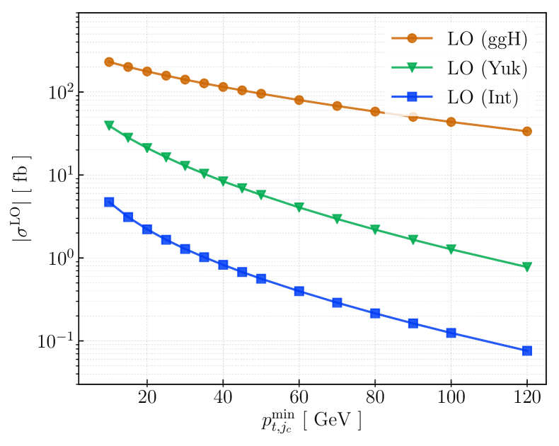
(a) Fiducial cross section (LO)

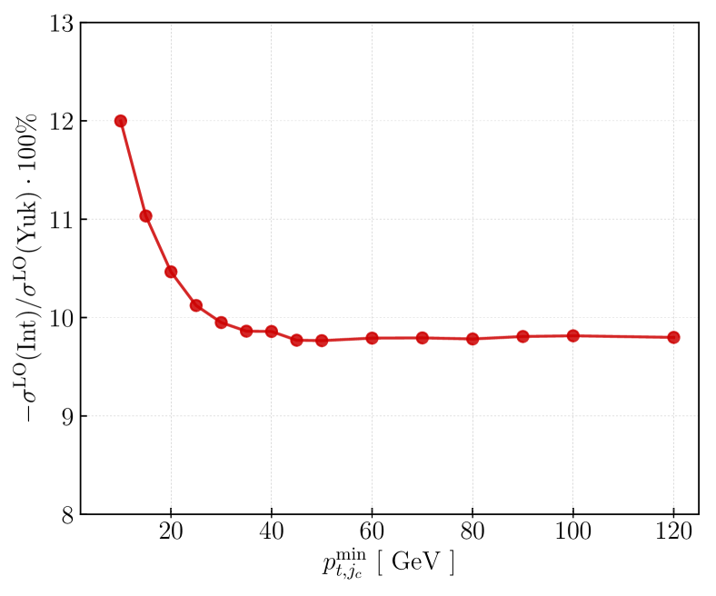
(b) Interference/Yukawa ratio

Figure 2: Leading-order cross sections computed for different values of the charm-jet $p_{t}$-cut. We show Yukawa-like (green) and $ggH$-like (orange) contributions as well as the absolute value of the interference (blue). In the right pane the ratio of the interference and the Yukawa-like fiducial cross section are shown.

We start by presenting fiducial cross sections for the three terms in Eq. (2) separately. Central values for all the cross sections presented below correspond to the renormalization and factorization scales set to $\mu_{F}=\mu_{R}=\mu=M_{H}$; subscripts and superscripts indicate shifts in central values if $\mu=M_{H}/2$ and $\mu=2M_{H}$ are used in the calculation. At leading order, we find

$$\sigma^{\rm LO}_{{ggH}}={} 176.6^{+47.6}_{-36.5}~{}{\rm fb}\,, \sigma^{\rm LO}_{{\rm Yuk}}={} 21.22^{+1.47}_{-1.67}~{}{\rm fb}\,, \sigma^{\rm LO}_{{\rm Int}}={} -2.21^{+0.29}_{-0.31}~{}{\rm fb}\,,$$ (39)

for the $ggH$-dependent cross section, the Yukawa-dependent cross section and the interference, respectively. In Figure 2 we show the comparison between $\mu=M_{H}$ cross sections and the interference in dependence on the cut of the charm jet transverse momentum. We observe that the ratio of the interference to the Yukawa-dependent contribution is about ten percent for all values of the $p_{t,j}$-cut.

At next-to-leading order the fiducial cross section for the interference term becomes

$$\sigma^{\rm NLO}_{{\rm Int}}={} -1.024(5)^{+0.224}_{-0.144}~{}{\rm fb}\,.$$ (40)

It follows from Eqs. (39,40) that the NLO QCD corrections decrease the absolute value of the leading-order interference by about fifty percent. The scale uncertainty appears to be reduced by about a factor 2. The NLO result for the interference is outside the leading-order scale-uncertainty interval, c.f. Eqs. (39,40), emphasizing the fact that the appearance of the logarithms of the charm mass in NLO QCD corrections to the interference makes the scale variation uncertainty of the leading-order result a very poor indicator of the theoretical uncertainty in this case.

$\Delta\sigma^{\rm NLO}~{}[~{}{\rm fb}~{}]$	$cg$	$cq$	$gg$	$cc$	${c\bar{c}}$	PDF	sum
const	$-1.63$	$0.13$	$2.33$	$0.01$	$-0.01$	$0.11$	$0.94$
$L$	$2.23$	$-$	$-6.33$	$-0.04$	$0.01$	$1.66$	$-2.47$
$L^{2}$	$-0.06$	$-$	$2.66$	$0.01$	$-0.08$	$-$	$2.52$
total	$0.54$	$0.13$	$-1.34$	$-0.02$	$-0.08$	$1.76$	$1.00$

Table 1: The NLO QCD corrections to the interference split according to partonic channels. The results are given in femtobarns. The column marked “PDF” refers to the PDF-scheme change discussed in Section 2. For each partonic channel we show ${\cal O}(L^{2})$, ${\cal O}(L)$ and ${\cal O}(L^{0})$ contributions where $L=\ln(M_{H}/m_{c})$.

It is instructive to separate the NLO contributions to the interference into parts that are independent of $m_{c}$ and parts that are logarithmically enhanced for all the partonic channels. The relevant results are shown in Table 1. We find that the largest contribution at NLO comes from the gluon-gluon channel which is enhanced by the large gluon luminosity. Also, the charm-gluon ($cg$) and the charm-quark channels ($cq$) provide relatively large contributions. Note that the $(cq)$ channel is free of logarithmic contributions since there are no singular limits that involve charm quarks. Contributions related to the PDF transformation do not feature the double-logarithmic part since the ${\cal O}(\ln^{2}m_{c})$ terms originate exclusively from soft-collinear limits that involve $c$-quarks.

It follows from Table 1 that double-logarithmic terms and single-logarithmic terms provide nearly equal, but opposite in sign, contributions to the NLO QCD interference. This cancellation between terms with different parametric dependence on $m_{c}$ should be considered as an artifact but it does emphasize that studying only the leading logarithmic ${\cal O}(\ln^{2}m_{c})$ contribution in this case is insufficient for phenomenology. We also note that the ${\cal O}(\ln^{2}m_{c})$ term in the $cg$ channel is quite small reflecting the fact that there is a very strong – but incomplete – cancellation between double-logarithmic contributions to real and virtual corrections in this case. Finally, we emphasize that it is unclear to what extent these various cancellations persist in higher orders; for this reason, a resummation of charm-mass logarithms for the interference contribution is desirable.

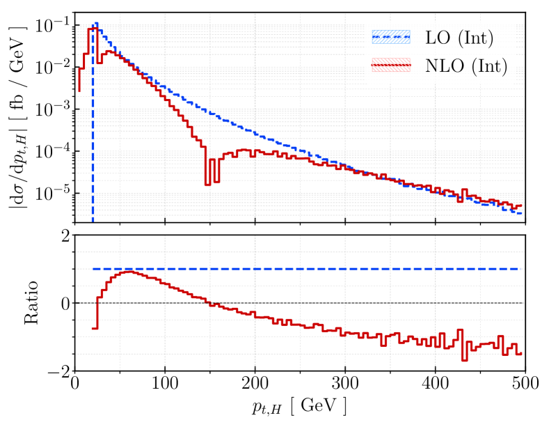
(a) Higgs-boson transverse momentum

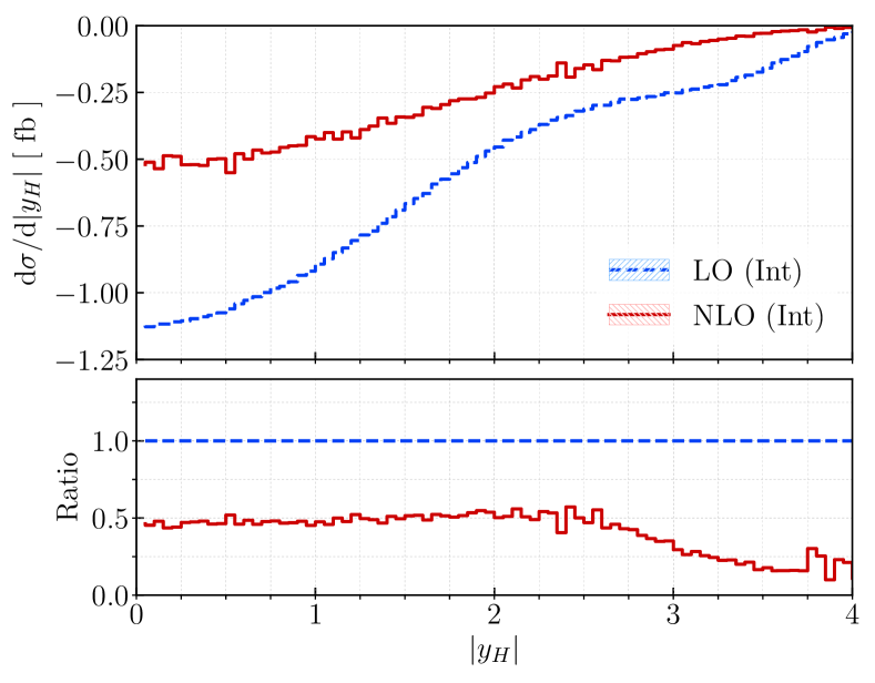
(b) Higgs-boson rapidity

Figure 3: The transverse momentum and rapidity distributions of the Higgs boson calculated at LO (blue) and NLO (red) for central scale choice. We only consider the interference contribution. We note that the absolute value of ${\rm d}\sigma_{\rm Int}/{\rm d}p_{t,H}$ is displayed in the left panel. This implies that this distribution actually changes sign at around $p_{t,H}\sim 150~{}{\rm GeV}$. The lower panels show ratios to the LO interference contribution.

We continue with the discussion of kinematic distributions. We focus on the transverse momentum and the rapidity distributions of Higgs bosons in the interference contribution to $pp\to Hc$ cross section. They are shown in Figure 3. We first discuss the transverse momentum distribution, Figure 3(a); when interpreting this figure it is important to recall that the absolute value of both LO and NLO distributions is plotted there and that the LO distribution is always negative. We observe in Figure 3(a) that the leading-order distribution (blue) is large and negative at small $p_{t,H}$; as $p_{t,H}$ increases, the distribution goes to zero. The NLO QCD corrections affect the shape of the $p_{t,H}$ distribution. Indeed, a sharp edge at $p_{t,H}=20$ GeV, present at leading order, gets smeared at NLO. At moderate values of transverse momenta $p_{t,H}\sim 60~{}{\rm GeV}$ the $K$-factor is equal to one, while there is a large ${\cal O}(+50\%)$ reduction at $p_{t,H}\sim 100~{}{\rm GeV}$. Second, at $p_{t,H}\sim 150~{}{\rm GeV}$ the NLO distribution goes through zero and becomes positive for larger values of $p_{t,H}$. Asymptotically, at even higher $p_{t,H}$ the LO and NLO distributions appear to be equal in absolute values but opposite in sign. Of course, all this happens at such high values of $p_{t,H}$ that are irrelevant for phenomenology, but it is quite a peculiar feature nevertheless.

Compared to Higgs transverse momentum distribution, the rapidity distribution of the Higgs boson in the interference contribution is much less volatile. Indeed, it follows from Figure 3(b) that the difference between leading and next-to-leading-order distributions is well-described by a constant $K$-factor all the way up to $|y_{H}|\sim 2$. Beyond this value of the rapidity, the NLO distribution goes to zero faster than the LO one.

6 Conclusions

Production of Higgs bosons in association with charm jets at the LHC is mediated by two distinct mechanisms, one that involves the charm Yukawa coupling and the other one that involves an effective ${ggH}$ vertex. Their interference involves a helicity flip and, for this reason, vanishes in the limit of massless charm quarks.

Since partonic cross sections are routinely computed for massless incoming partons and since the charm quark appears in the initial state in the main process $cg\to Hc$, it is interesting to understand how to circumvent the problem of having to deal with a massive parton in the initial state and to provide reliable estimate of the interference contribution.

We have addressed this problem by studying the $m_{c}\to 0$ limit of the helicity-flipping interference contribution including NLO QCD corrections. We have shown that the factorization of quasi-collinear and quasi-soft singularities in this case differs from the canonical pattern. We used explicit expressions for real and virtual matrix elements to extract logarithms of the charm quark mass and, having accomplished this, took the $m_{c}\to 0$ limit in the remaining parts of the computation. We removed parts of the ${\cal O}(\ln m_{c})$ contributions by expressing results through conventional ${\overline{\rm MS}}$ parton distribution functions valid for massless partons. Nevertheless, given an unconventional behavior of the interference in quasi-soft and quasi-collinear limits, logarithms of the charm quark mass survive in the final result for the NLO QCD corrections.

We have found that the absolute value of the leading-order interference is reduced by about fifty percent once NLO QCD corrections are accounted for. This significant but still “perturbatively acceptable” reduction is the result of a very strong cancellation between terms that involve double and single logarithms of the charm quark mass. We have observed that the NLO QCD corrections to the interference are kinematics-dependent and may change shapes of certain kinematic distributions in a significant way.

Higgs boson production in association with a charm jet is a promising way to study charm Yukawa coupling at the LHC Brivio:2015fxa . The interference contribution, that is estimated to be about $10$ percent of the Yukawa contribution at leading order, could have been perturbatively unstable given the required helicity flip and an unconventional pattern of quasi-soft and quasi-collinear limits. We addressed this question by performing a dedicated NLO QCD computation for the interference term and did not find a strong indication that this might be the case. Nevertheless, the moderate size of the NLO QCD corrections is the consequence of a very strong cancellations between double and single logarithms of the charm mass. It is unclear if this cancellation persists in higher orders. Hence, resummation of ${\cal O}(\ln m_{c})$-enhanced terms for this process is quite desirable.

Acknowledgments  This research is partially supported by the Deutsche Forschungsgemeinschaft (DFG, German Research Foundation) under grant 396021762 - TRR 257.

Appendix A Extraction of the ${\cal O}(\ln m_{c})$-enhanced contributions in the real corrections

In this appendix we describe a procedure to extract ${\cal O}(\ln m_{c})$ contributions to real emission corrections. They arise because of the quasi-singular behavior of real emission amplitudes in the soft or collinear limits involving charm quarks. The potential singularities in these limits are regulated by the charm mass leading to an appearance of ${\cal O}(\ln m_{c})$-enhanced terms when integrated over relevant phase spaces. To extract logarithms of $m_{c}$, we subtract approximate expressions from exact matrix elements that make the difference integrable in the $m_{c}\to 0$ limit and integrate the subtraction terms over unresolved phase space to explicitly extract logarithms of $m_{c}$.

As an example, we consider the gluon-gluon partonic channel, i.e.

$$g(p_{1})+g(p_{2})\longrightarrow H(p_{H})+c(p_{3})+\bar{c}(p_{4})\,,$$ (41)

and discuss the extraction of ${\cal O}(\ln m_{c})$ terms in detail. This channel is suitable for such a discussion since, if the charm-quark mass is kept finite, it is free of soft and collinear divergences. Hence, all relevant contributions can be computed numerically for small but finite $m_{c}$, and used to validate formulas where logarithms of $m_{c}$ have been extracted and $m_{c}\to 0$ limit has been taken where appropriate.

As we already mentioned in the main text, we use the nested soft-collinear subtraction scheme which, at this order, is equivalent to the FKS subtraction scheme Frixione:1995ms ; Frixione:1997np . The details of the subtraction scheme can be found in the literature Caola:2017dug ; Caola:2019nzf ; Caola:2019pfz ; Asteriadis:2019dte and we do not repeat this discussion here. Nevertheless, the treatment of quasi-collinear and quasi-soft singularities related to the emission of massive charm quarks is new and requires an explanation.

We focus on the interference contribution between the Yukawa-like and the ${ggH}$-like production mechanisms in the process Eq. (41). The interference term is non-zero only if helicity flip on the charm line occurs. Furthermore, the presence of such a helicity flip causes the usual factorization formulas to break down and the singular limits need to be explicitly analyzed. We note that, thanks to the symmetry of the squared amplitude for the process in Eq. (41) under the exchange of $c$ and $\bar{c}$, we can consider only the case where $\bar{c}$ quark becomes soft or quasi-collinear to one of the other partons. The case when both $c$ and $\bar{c}$ become unresolved is impossible since we require a charm jet in the final state.

The quasi-singular limits which appear in this channel are related to the soft-quark limit $S_{4}$ with $E_{4}\sim m_{c}$ and the three collinear limits $C_{4i}$ with $i=1,2,3$ where $({p_{4}\!\cdot\!p_{i}})\sim m_{c}^{2}$. Performing an iterative subtraction of these singular limits, we find

$$\begin{split}\langle F_{\rm LM}(1_{g},2_{g};3_{c},4_{\bar{c}})\rangle={}&\sum_{i=1}^{3}\langle(1-C_{4i})(1-S_{4})\omega^{(i)}_{123}F_{\rm LM}(1_{g},2_{g};3_{c},4_{\bar{c}})\rangle\\ &+\langle C_{4i}(1-S_{4})\omega^{(i)}_{123}F_{\rm LM}(1_{g},2_{g};3_{c},4_{\bar{c}})\rangle\\ &+\langle S_{4}F_{\rm LM}(1_{g},2_{g};3_{c},4_{\bar{c}})\rangle\,,\end{split}$$ (42)

where the first term on the right-hand side denotes the fully-regulated contribution and the second and third terms are the collinear and the soft integrated subtraction terms. The factors $\omega^{(i)}_{123}$ are the weights that describe various collinear sectors. They read

$$\omega^{(i)}_{123}={} \frac{1}{\rho_{4i}}\cdot\left[\frac{1}{\rho_{41}}+\frac{1}{\rho_{42}}+\frac{1}{\rho_{43}}\right]^{-1}\,,$$ (43)

with $\rho_{4i}=1-\cos\theta_{4i}$. We note that, since all $m_{c}\to 0$ singularities are subtracted in the fully-regulated term in Eq. (42), the $m_{c}\to 0$ limit can be immediately taken there. On the other hand, the integrated subtraction terms in the second line of Eq. (42) require care to capture all the ${\cal O}(\ln m_{c})$-terms and constants which survive the $m_{c}\to 0$ limit.

In the remaining part of this section, we discuss in detail the integration of the subtraction terms. We first focus on the soft subtraction term, i.e. the last term in Eq. (42), and then the integration of the collinear subtraction term, i.e. the first term in the second line of Eq. (42).

A.1 Integration of the soft-quark subtraction terms

Consider the soft-quark subtraction term

$$\langle S_{4}F_{\rm LM}(1_{g},2_{g};3_{c},4_{\bar{c}})\rangle\,.$$ (44)

To compute it, we need to know the behavior of the amplitude in the limit $p_{4}\sim m_{c}\to 0$ and then integrate it over the phase space of the charm anti-quark with momentum $p_{4}$.

Although, normally, soft (gluon) emissions factorize into a product of an eikonal factor and a tree-level matrix element squared, a similar formula for soft-quark emission, relevant for helicity-flipping processes, does not exist. Hence, we determine the soft-quark limit of the interference by studying an explicit expression of the amplitude for the process in Eq. (41) in the limit $p_{4}\sim m_{c}\to 0$. We find

$$\begin{split}S_{4}{\rm Int}\left[|\mathcal{M}(1_{g},2_{g};3_{c},4_{\bar{c}})|^{2}\right]\sim{}&\frac{(2C_{F}-C_{A})({p_{1}\!\cdot\!p_{2}})}{({p_{1}\!\cdot\!p_{4}})({p_{2}\!\cdot\!p_{4}})}F_{12}(p_{1},p_{2},p_{3})\\ &+\frac{C_{A}({p_{1}\!\cdot\!p_{3}})}{({p_{1}\!\cdot\!p_{4}})(m_{c}^{2}+{p_{3}\!\cdot\!p_{4}})}\;F_{13}(p_{1},p_{2},p_{3})\\ &+\frac{C_{A}({p_{2}\!\cdot\!p_{3}})}{({p_{2}\!\cdot\!p_{4}})(m_{c}^{2}+{p_{3}\!\cdot\!p_{4}})}F_{23}(p_{1},p_{2},p_{3})\,,\end{split}$$ (45)

where functions $F_{ij}$ depend on the momenta $p_{1}$, $p_{2}$ and $p_{3}$ only. We emphasize that these functions are different from the leading-order interference contribution. The massless limit, $m_{c}\to 0$, can be now taken everywhere except for the eikonal factors and the phase-space measure of the unresolved parton $[{\rm d}{p_{4}}]$.

We write the integrated soft subtraction term as follows

$$\begin{split}\langle S_{4}F_{\rm LM}(1_{g},2_{g};3_{c},4_{\bar{c}})\rangle={}&(2C_{F}-C_{A})\langle F_{12}(p_{1},p_{2},p_{3})\cdot\int\frac{[{\rm d}{p_{4}}]({p_{1}\!\cdot\!p_{2}})}{({p_{1}\!\cdot\!p_{4}})({p_{2}\!\cdot\!p_{4}})}\rangle\\ &+C_{A}\langle F_{13}(p_{1},p_{2},p_{3})\cdot\int\frac{[{\rm d}{p_{4}}]({p_{1}\!\cdot\!p_{3}})}{({p_{1}\!\cdot\!p_{4}})(m_{c}^{2}+{p_{3}\!\cdot\!p_{4}})}\rangle\\ &+C_{A}\langle F_{23}(p_{1},p_{2},p_{3})\cdot\int\frac{[{\rm d}{p_{4}}]({p_{2}\!\cdot\!p_{3}})}{({p_{2}\!\cdot\!p_{4}})(m_{c}^{2}+{p_{3}\!\cdot\!p_{4}})}\rangle\,,\end{split}$$ (46)

where $\langle\ldots\rangle$ denotes the phase space integration and the relevant soft integrals can be found in Appendix B. We stress that soft integrals are finite in four dimensions since they are naturally regulated by the charm-quark mass $m_{c}$.

A.2 Integration of the quasi-collinear subtraction terms

In this subsection, we discuss how to define and compute the soft-subtracted quasi-collinear limits of the interference contribution using the process in Eq. (41) as an example. We focus on the sector $43$ where $c$ and $\bar{c}$ become collinear to each other. The relevant quantity reads

$$\langle C_{43}(1-S_{4})F_{\rm LM}(1_{g},2_{g};3_{c},4_{\bar{c}})\rangle\,.$$ (47)

To proceed further, we split the above formula into collinear and soft-collinear terms

$$\langle C_{43}(1-S_{4})F_{\rm LM}(1_{g},2_{g};3_{c},4_{\bar{c}})\rangle={} \langle C_{43}F_{\rm LM}(1_{g},2_{g};3_{c},4_{\bar{c}})\rangle-\langle C_{43}S_{4}F_{\rm LM}(1_{g},2_{g};3_{c},4_{\bar{c}})\rangle\,.$$ (48)

We first discuss the collinear subtraction term $\langle C_{43}F_{\rm LM}(1_{g},2_{g};3_{c},4_{\bar{c}})\rangle$ defined as follows

$$\begin{split}\langle C_{43}F_{\rm LM}(1_{g},2_{g};3_{c},4_{\bar{c}})\rangle={}&\sum_{i=1}^{2}\int[{\rm d}{p_{H}}][{\rm d}{p_{3}}][{\rm d}{p_{4}}](2\pi)^{4}\delta\left(p_{12}-p_{H}-p_{3}-{\bar{p}_{4}}\right)\\ &\hphantom{\sum_{i=1}^{2}\langle}\times\frac{1}{(p_{3}+p_{4})^{2}}\frac{{p_{i}\!\cdot\!p_{3}}}{p_{i}\!\cdot\!{\bar{p}_{4}}}{C}_{i}(1_{g},2_{g},3_{c},\bar{4}_{\bar{c}})\,,\end{split}$$ (49)

In the above equation, the functions ${C}_{1,2}$ depend on the momenta $p_{1}$, $p_{2}$, $p_{3}$ and $\bar{p}_{4}$. The bar over momentum $p_{4}$ indicates that the relevant collinear limit has been taken, i.e.

$$C_{43}p_{4}=(E_{4},\beta_{4}\vec{n}_{3})\equiv\bar{p}_{4}\,.$$ (50)

Note that in Eq. (50) $\beta_{4}=\sqrt{1-m_{c}^{2}/E_{4}^{2}}$ is the velocity of $\bar{c}$ and $\vec{n}_{3}$ is a unit vector pointing in the direction of momentum $\vec{p}_{3}$. We note that in Eq. (49) the massless limit $m_{c}\to 0$ has not been taken. We also note that the functions $C_{1,2}$ are regular in the soft-quark limit, $E_{4}\to m_{c}\sim 0$.

Our goal is to extract all ${\cal O}(\ln m_{c})$ terms arising from Eq. (49) and take the massless limit after that. To do so, we add and subtract the soft limits of the functions $C_{i}$

$${C}_{i}(1_{g},2_{g},3_{c},\bar{4}_{\bar{c}})={} \big{[}{C}_{i}(1_{g},2_{g},3_{c},\bar{4}_{\bar{c}})-{C}_{i,\rm soft}(1_{c},2_{g},3_{c})\big{]}+{C}_{i,\rm soft}(1_{c},2_{g},3_{c})\,,$$ (51)

where ${C}_{i,\rm soft}(1_{c},2_{g},3_{c})={C}_{i}(1_{g},2_{g},3_{c},0)$. The above procedure splits the integral in Eq. (49) into two parts: the regulated integral that contains the expression in the square bracket in Eq. (51) and the soft part. In the regulated part, the soft divergence at $E_{4}=0$ has been regularized. This implies that, after integrating $1/(p_{3}+p_{4})^{2}$ over the relative angle between $p_{3}$ and $p_{4}$ and extracting logarithms of $m_{c}$ from this angular integral, we can set $m_{c}$ to zero everywhere else right away. We obtain

$$\langle C_{43}F_{\rm LM}(1_{g},2_{g};3_{c},4_{\bar{c}})\rangle_{\rm reg}={} \frac{1}{(2\pi)^{2}}\sum_{i=1}^{2}\int[{\rm d}{p_{H}}][{\rm d}{p_{3}}](2\pi)^{4}\delta\left(p_{12}-p_{H}-p_{34}\right)$$

$$\int_{0}^{1}\frac{z\,{\rm d}{z}}{1-z}\Big{[}C_{i}(1_{g},2_{g},z34,(1-z)34)-{C}_{i,\rm soft}(1_{c},2_{g},z34)\Big{]}$$

$$\times\Big{[}\ln(2E_{34}/m_{c})+\ln(1-z)+\ln(z)\Big{]}\,,$$ (52)

where we have used the fact that in $m_{c}\to 0$ limit we can write $p_{3}=zp_{34}$ and $\bar{p}_{4}=(1-z)p_{34}$ for $p_{34}^{2}=0$.

We will now discuss the soft part of the collinear subtraction term. It reads

$$\begin{split}\langle C_{43}F_{\rm LM}(1_{g},2_{g};3_{c},4_{\bar{c}})\rangle_{\rm soft}={}&\sum_{i=1}^{2}\int[{\rm d}{p_{H}}][{\rm d}{p_{3}}][{\rm d}{p_{4}}](2\pi)^{4}\delta\left(p_{12}-p_{H}-p_{3}-{\bar{p}_{4}}\right)\\ &\times\frac{1}{(p_{3}+p_{4})^{2}}\frac{{p_{i}\!\cdot\!p_{3}}}{p_{i}\!\cdot\!{\bar{p}_{4}}}{C}_{i,\rm soft}(1_{c},2_{g},3_{c})\,.\end{split}$$ (53)

We emphasize that this term still contains soft singularity and, for this reason, the $m_{c}\to 0$ limit cannot be taken. However, it is convenient to combine this integral with the soft-collinear subtraction term $\langle C_{43}S_{4}F_{\rm LM}(1_{g},2_{g};3_{c},4_{\bar{c}})\rangle$, c.f. Eq. (48); if this is done, the required computations simplify significantly.

The soft-collinear integrated subtraction term in sector 43 reads

$$\begin{split}\langle C_{43}S_{4}F_{\rm LM}(1_{g},2_{g};3_{c},4_{\bar{c}})\rangle={}&\sum_{i=1}^{2}\int[{\rm d}{p_{H}}][{\rm d}{p_{3}}][{\rm d}{p_{4}}](2\pi)^{4}\delta\left(p_{12}-p_{H}-p_{3}\right)\\ &\hphantom{\sum_{i=1}^{2}}\times\frac{2C_{A}F_{i3}(p_{1},p_{2},p_{3})}{(p_{3}+p_{4})^{2}}\frac{{p_{i}\!\cdot\!p_{3}}}{p_{i}\!\cdot\!{\bar{p}_{4}}}\,.\end{split}$$ (54)

To derive this result we used the soft-limit of the interference amplitude reported in Eq. (45). We emphasize that, since the soft operator is present on the left hand side in the above equation, the soft-quark momentum $p_{4}$ is removed from the energy-momentum conserving delta-function. Moreover, since

$$C_{i,\rm soft}(1_{c},2_{g},3_{c})={} 2C_{A}F_{i3}(p_{1},p_{2},p_{3})\,,$$ (55)

the two integrals in Eqs. (53,54) appear to be the same up to the argument of the delta-functions. We combine the two integrals and find

$$\langle C_{43}F_{\rm LM}(1_{g},2_{g};3_{c}, 4_{\bar{c}})\rangle_{\rm soft}-\langle C_{43}S_{4}F_{\rm LM}(1_{g},2_{g};3_{c},4_{\bar{c}})\rangle={}$$

$$={} \sum_{i=1}^{2}\int[{\rm d}{p_{H}}][{\rm d}{p_{3}}][{\rm d}{p_{4}}](2\pi)^{4}\Big{[}\delta\left(p_{12}-p_{H}-p_{3}-\bar{p}_{4}\right)-\delta\left(p_{12}-p_{H}-p_{3}\right)\Big{]}$$

$$\hphantom{\sum_{i=1}^{2}}\times\frac{2C_{A}F_{i3}(p_{1},p_{2},p_{3})}{(p_{3}+p_{4})^{2}}\frac{{p_{i}\!\cdot\!p_{3}}}{p_{i}\!\cdot\!{\bar{p}_{4}}}\,.$$ (56)

To proceed further, we note that it is straightforward to integrate over directions of the quark with momentum $p_{4}$ but integration over its energy is more involved. It is convenient to split the $E_{4}$ integration into two regions by introducing an auxiliary parameter $\sigma$

$$1={} \Theta(E_{4}-\sigma)+\Theta(\sigma-E_{4})\,.$$ (57)

We choose $\sigma$ to satisfy the following inequality $m_{c}\ll\sigma\ll E_{3}$. For small energies, $E_{4}<\sigma\ll E_{3}$, we can drop the momentum $\bar{p}_{4}$ from the energy momentum conserving delta-function which leads to

$$\begin{split}\Big{[}&\delta\left(p_{12}-p_{H}-p_{3}-\bar{p}_{4}\right)\big{[}\Theta(E_{4}-\sigma)+\Theta(\sigma-E_{4})\big{]}-\delta\left(p_{12}-p_{H}-p_{3}\right)\Big{]}={}\\ &\hskip 28.45274pt={}\Big{[}\delta\left(p_{12}-p_{H}-p_{3}-\bar{p}_{4}\right)-\delta\left(p_{12}-p_{H}-p_{3}\right)\Big{]}\Theta(E_{4}-\sigma)+\mathcal{O}(\sigma/E_{3})\,.\end{split}$$ (58)

This relation implies that the integrand in Eq. (A.2) is non-vanishing only in the high-energy domain where $E_{4}>\sigma\gg m_{c}$ and, therefore, the limit $m_{c}\to 0$ can be taken. This leads to the following expression

$$\langle C_{43}F_{\rm LM}(1_{g}, 2_{g};3_{c},4_{\bar{c}})\rangle_{\rm soft}-\langle C_{43}S_{4}F_{\rm LM}(1_{g},2_{g};3_{c},4_{\bar{c}})\rangle={}$$

$$= \frac{C_{A}}{(2\pi)^{2}}\sum\limits_{i=1}^{2}\int[{\rm d}p_{H}][{\rm d}p_{34}](2\pi)^{4}\delta(p_{12}-p_{H}-p_{34})$$

$$\Bigg{\{}\int\limits_{z_{\rm min}}^{z_{\rm max}}\frac{{\rm d}z}{1-z}\ln\left(\frac{2E_{34}(1-z)z}{m_{c}}\right)\Big{[}z\theta(z)F_{i3}(p_{1},p_{2},zp_{34})-F_{i3}(p_{1},p_{2},p_{34})\Big{]}$$

$$+\int\limits_{z_{\rm min}}^{z_{\rm max}}\frac{{\rm d}z}{1-z}\ln\big{(}(2-z)z\big{)}F_{i3}(p_{1},p_{2},p_{34})\Bigg{\}}.$$ (59)

To arrive at Eq. (A.2) we introduced the four-momentum $p_{34}=p_{3}+\bar{p}_{4}$ and a variable $z$ such that $p_{3}=zp_{34}$ in terms that contain the delta-function $\delta{(p_{12}-p_{H}-p_{3}-\bar{p}_{4})}$. In terms that contain the delta-function $\delta{(p_{12}-p_{H}-p_{3})}$, we set $(1-z)=E_{4}/E_{3}$, rename $p_{3}$ into $p_{34}$ and set $\sigma\to 0$. The lower integration boundary $z_{\rm min}$ is given by $z_{\rm min}=1-{E_{\rm max}}/E_{34}<0$.

In total, the integrated collinear term $\langle C_{43}(1-S_{4})F_{\rm LM}(1_{g},2_{g};3_{c},4_{\bar{c}})\rangle$ is given by a sum of expressions in Eqs. (A.2,A.2). We describe a numerical check of validity of this result in the following section.

A.3 Numerical checks

Since the cross section of the gluon-gluon channel, Eq. (41), is finite as long as we keep the non-zero charm mass, analytical results derived in the previous section can be checked numerically by computing $\sigma_{gg\to Hc\bar{c}}$ explicitly for small values of the charm mass without any approximation.

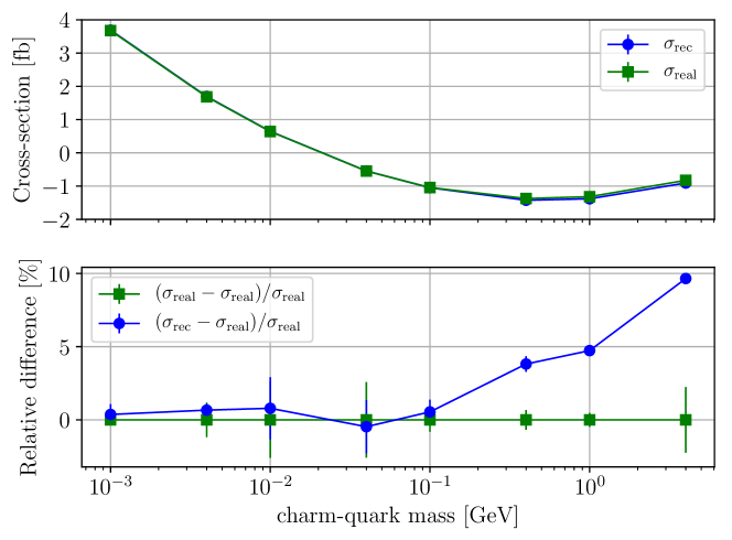
Figure 4: The cross section of the $gg\to H{c\bar{c}}$ process calculated by a direct integration of the matrix element with non-zero charm-quark mass, $\sigma_{\rm real}$ (green rectangles), and reconstructed using procedure described in previous subsections, $\sigma_{\rm rec}$ (blue circles). We employ the same parameters and kinematic constraints as in the main text.

The comparison is shown in Figure 4. We use fiducial cuts described in the main text and compare hadronic contributions to the interference for $gg$ partonic channel computed in two different ways. Green points (rectangles) show the results of the computation without any approximation, i.e. by directly integrating the matrix element squared. Blue points (circles) show the results of the computation that relies on the expansion around $m_{c}\to 0$ limit, as described in previous subsections. The two results should agree for small values of $m_{c}$. The upper panel of Figure 4 shows the absolute values of the interference cross section in the $gg$ partonic channel obtained with the two methods, while their difference is shown in the lower panel. We see a better and better agreement between the two results as we mover to smaller and smaller values of the charm-quark mass. This indicates that the $m_{c}$-dependence of the interference contribution is properly reconstructed.

Appendix B Soft-quark integrals

In this section we list integrals that are required for the integrated soft-quark subtraction terms. We need a number of integrals depending on the type and configuration of the emitters $p_{a}$ and $p_{b}$ as well as the propagator appearing in the eikonal factor.

We note that we are interested only in the terms that contain logarithms of the charm-quark mass and constant terms, but we drop all power-suppressed terms which vanish in the $m_{c}\to 0$ limit. All integrals are computed in $d=4$ dimensions since all singularities are naturally regulated by the charm-quark mass.

The phase-space measure for a massive-quark emission, $p_{4}^{2}=m_{c}^{2}$, reads

$$[{\rm d}{p_{4}}]={} \frac{k_{4}^{2}{\rm d}{k_{4}}}{2E_{4}}\frac{{\rm d}\Omega^{(3)}}{(2\pi)^{3}}\Theta({E_{\rm max}}-E_{4})\Theta(E_{4}-m_{c})\,,$$ (60)

where $k_{4}$ is the length of $\vec{p}_{4}$ momentum, ${\rm d}\Omega^{(3)}$ denotes angular integration and ${E_{\rm max}}$ is the usual energy cutoff of the nested soft-collinear subtraction scheme. In the remaining part of this section, we list soft-quark integrals that are needed to obtain integrated soft-quark subtraction terms, see Section A.1 for details.

Two massless emitters:

Two emitters $a,b$ have four-momenta $p_{a}=E_{a}(1,\vec{n}_{a})$ and $p_{b}=E_{b}(1,\vec{n}_{b})$, respectively. Both four-momenta are light-like $p_{a}^{2}=p_{b}^{2}=0$. Vectors $\vec{n}_{a}$ and $\vec{n}_{b}$ describe direction of flight of the emitters; we refer to the opening angle between $\vec{n}_{a}$ and $\vec{n}_{b}$ as $\theta_{ab}$.

The soft integral reads

$$\int\frac{[{\rm d}{p_{4}}]({p_{a}\!\cdot\!p_{b}})}{({p_{a}\!\cdot\!p_{4}})({p_{b}\!\cdot\!p_{4}})}={} \frac{1}{(2\pi)^{2}}\left[\ln^{2}(2s_{ab}{E_{\rm max}}/m_{c})-\frac{\pi^{2}}{12}+\frac{1}{2}{{\rm Li}_{2}}(c_{ab}^{2})\right]\,,$$ (61)

where we used $s_{ab}=\sin(\theta_{ab}/2)$ and $c_{ab}=\cos(\theta_{ab}/2)$.

One massive and one massless emitters:

Two emitters $a,b$ have four-momenta $p_{a}=E_{a}(1,\vec{n}_{a})$ and $p_{b}=E_{b}(1,\beta_{b}\vec{n}_{b})$, respectively. They satisfy $p_{a}^{2}=0$ and $p_{b}^{2}=m_{c}^{2}$. We refer to the opening angle between $\vec{n}_{a}$ and $\vec{n}_{b}$ as $\theta_{ab}$. We require three soft integrals of this type

$$\begin{split}&\int\frac{[{\rm d}{p_{4}}]({p_{a}\!\cdot\!p_{b}})}{({p_{a}\!\cdot\!p_{4}})(m_{c}^{2}+{p_{b}\!\cdot\!p_{4}})}={}\frac{1}{(2\pi)^{2}}\bigg{[}\ln^{2}(2s_{ab}{E_{\rm max}}/m_{c})-\frac{\pi^{2}}{12}\\ &\hphantom{\frac{1}{(2\pi)^{2}}\bigg{[}}+{{\rm Li}_{2}}(-{E_{\rm max}}/E_{b})+\frac{1}{2}{{\rm Li}_{2}}(c_{ab}^{2})\bigg{]}\,,\\ &\int\frac{[{\rm d}{p_{4}}]({p_{a}\!\cdot\!p_{b}})}{({p_{a}\!\cdot\!p_{4}})({p_{b}\!\cdot\!p_{4}})}=\frac{1}{(2\pi)^{2}}\bigg{[}\ln^{2}(2s_{ab}{E_{\rm max}}/m_{c})+\frac{1}{4}{{\rm Li}_{2}}(-{E_{\rm max}}^{2}/E_{b}^{2})\\ &\hphantom{\frac{1}{(2\pi)^{2}}\bigg{[}}-\frac{\pi^{2}}{12}+\frac{1}{2}{{\rm Li}_{2}}(c_{ab}^{2})\bigg{]}\,,\\ &\int\frac{[{\rm d}{p_{4}}]({p_{a}\!\cdot\!p_{b}})}{({p_{a}\!\cdot\!p_{4}})(m_{c}^{2}-{p_{b}\!\cdot\!p_{4}})}=\frac{1}{(2\pi)^{2}}\bigg{[}-\ln^{2}(2s_{ab}{E_{\rm max}}/m_{c})+{{\rm Li}_{2}}(1-{E_{\rm max}}/E_{b})\\ &\hphantom{\frac{1}{(2\pi)^{2}}\bigg{[}}-\frac{1}{2}{{\rm Li}_{2}}(c_{ab}^{2})+\ln({E_{\rm max}}/E_{b})\ln({E_{\rm max}}/E_{b}-1)-\frac{\pi^{2}}{12}\bigg{]}\,,\end{split}$$ (62)

where we used $s_{ab}=\sin(\theta_{ab}/2)$ and $c_{ab}=\cos(\theta_{ab}/2)$.

Two massive emitters:

Two emitters $a,b$ have four-momenta $p_{a}=E_{a}(1,\beta_{a}\vec{n}_{a})$ and $p_{b}=E_{b}(1,\beta_{b}\vec{n}_{b})$, respectively. They satisfy $p_{a}^{2}=p_{b}^{2}=m_{c}^{2}$. We refer to the opening angle between $\vec{n}_{a}$ and $\vec{n}_{b}$ as $\theta_{ab}$. In this case, we use ${E_{\rm max}}=E_{a}$. We find

$$\begin{split}&\int\frac{[{\rm d}{p_{4}}]({p_{a}\!\cdot\!p_{b}})}{(m_{c}^{2}-{p_{a}\!\cdot\!p_{4}})(m_{c}^{2}+{p_{b}\!\cdot\!p_{4}})}={}\frac{1}{(2\pi)^{2}}\bigg{[}-\ln^{2}(2s_{ab}{E_{\rm max}}/m_{c})-\frac{\pi^{2}}{12}\\ &\hphantom{\frac{1}{(2\pi)^{2}}\bigg{[}}-\frac{1}{2}{{\rm Li}_{2}}(c_{ab}^{2})-{{\rm Li}_{2}}(-{E_{\rm max}}/E_{b})\bigg{]}\,,\\ &\int\frac{[{\rm d}{p_{4}}]({p_{a}\!\cdot\!p_{b}})}{(m_{c}^{2}-{p_{a}\!\cdot\!p_{4}})(m_{c}^{2}-{p_{b}\!\cdot\!p_{4}})}=\frac{1}{(2\pi)^{2}}\bigg{[}\ln^{2}(2{E_{\rm max}}/m_{c})+\frac{\pi^{2}}{4}\bigg{]}\,,\end{split}$$ (63)

where we used $s_{ab}=\sin(\theta_{ab}/2)$ and $c_{ab}=\cos(\theta_{ab}/2)$.

References

- (1) M. Aaboud et al. [ATLAS], Phys. Lett. B 786 (2018), 59-86
- (2) A. M. Sirunyan et al. [CMS], Phys. Rev. Lett. 121 (2018) no.12, 121801
- (3) M. Aaboud et al. [ATLAS], Phys. Rev. D 99 (2019), 072001
- (4) A. M. Sirunyan et al. [CMS], JHEP 06 (2019), 093
- (5) G. Aad et al. [ATLAS], Phys. Lett. B 812 (2021), 135980
- (6) A. M. Sirunyan et al. [CMS], Phys. Rev. Lett. 122 (2019) no.2, 021801
- (7) G. Perez, Y. Soreq, E. Stamou and K. Tobioka, Phys. Rev. D 93 (2016) no.1, 013001
- (8) A. L. Kagan, G. Perez, F. Petriello, Y. Soreq, S. Stoynev and J. Zupan, Phys. Rev. Lett. 114 (2015) no.10, 101802
- (9) T. Modak and R. Srivastava, Mod. Phys. Lett. A 32 (2017) no.03, 1750004
- (10) M. König and M. Neubert, JHEP 08 (2015), 012
- (11) F. Bishara, U. Haisch, P. F. Monni and E. Re, Phys. Rev. Lett. 118 (2017) no.12, 121801
- (12) I. Brivio, F. Goertz and G. Isidori, Phys. Rev. Lett. 115 (2015) no.21, 211801
- (13) A. A. Penin, Phys. Lett. B 745 (2015), 69-72 [erratum: Phys. Lett. B 751 (2015), 596-596; erratum: Phys. Lett. B 771 (2017), 633-634]
- (14) K. Melnikov and A. Penin, JHEP 05 (2016), 172
- (15) Z. L. Liu and M. Neubert, JHEP 04 (2020), 033
- (16) Z. L. Liu, B. Mecaj, M. Neubert and X. Wang, JHEP 01 (2021), 077
- (17) E. Laenen, J. Sinninghe Damsté, L. Vernazza, W. Waalewijn and L. Zoppi, [arXiv:2008.01736].
- (18) S. Catani, S. Dittmaier and Z. Trocsanyi, Phys. Lett. B 500 (2001), 149-160
- (19) S. Frixione, JHEP 11 (2019), 158.
- (20) F. Caola, K. Melnikov and R. Röntsch, Eur. Phys. J. C 77 (2017) no.4, 248
- (21) F. Caola, K. Melnikov and R. Röntsch, Eur. Phys. J. C 79 (2019) no.5, 386
- (22) F. Caola, K. Melnikov and R. Röntsch, Eur. Phys. J. C 79 (2019) no.12, 1013
- (23) K. Asteriadis, F. Caola, K. Melnikov and R. Röntsch, Eur. Phys. J. C 80 (2020) no.1, 8
- (24) S. Frixione, Z. Kunszt and A. Signer, Nucl. Phys. B 467 (1996), 399-442
- (25) S. Frixione, Nucl. Phys. B 507 (1997), 295-314
- (26) A. Behring and W. Bizoń, JHEP 01 (2020), 189
- (27) S. Catani and M. H. Seymour, Nucl. Phys. B 485 (1997), 291-419 [erratum: Nucl. Phys. B 510 (1998), 503-504]
- (28) G. Passarino and M. J. G. Veltman, Nucl. Phys. B 160 (1979), 151-207
- (29) R. Mondini, U. Schubert and C. Williams, JHEP 12 (2020), 058
- (30) S. Catani, Phys. Lett. B 427 (1998), 161-171
- (31) R. Mertig, M. Bohm and A. Denner, Comput. Phys. Commun. 64 (1991), 345-359
- (32) V. Shtabovenko, R. Mertig and F. Orellana, Comput. Phys. Commun. 256 (2020), 107478
- (33) H. H. Patel, Comput. Phys. Commun. 197 (2015), 276-290
- (34) A. Buckley, J. Ferrando, S. Lloyd, K. Nordström, B. Page, M. Rüfenacht, M. Schönherr and G. Watt, Eur. Phys. J. C 75 (2015), 132
- (35) R. D. Ball et al. [NNPDF], Eur. Phys. J. C 77 (2017) no.10, 663
- (36) K. G. Chetyrkin, J. H. Kuhn and M. Steinhauser, Comput. Phys. Commun. 133 (2000), 43-65
- (37) F. Herren and M. Steinhauser, Comput. Phys. Commun. 224 (2018), 333-345