figurec \newwatermark[firstpage,color=gray!90,angle=0,scale=0.28, xpos=0in,ypos=-5in]*correspondence: v.liventsev@tue.nl
Neurogenetic Programming Framework
for Explainable Reinforcement Learning
Abstract
Automatic programming, the task of generating computer programs compliant with a specification without a human developer, is usually tackled either via genetic programming methods based on mutation and recombination of programs, or via neural language models. We propose a novel method that combines both approaches using a concept of a virtual neuro-genetic programmer 111not to be confused with neuroevolution [1]: using evolutionary methods as an alternative to gradient descent for neural network training, or scrum team. We demonstrate its ability to provide performant and explainable solutions for various OpenAI Gym tasks, as well as inject expert knowledge into the otherwise data-driven search for solutions. Source code is available at https://github.com/vadim0x60/cibi
Neurogenetic Programming Framework
Keywords Reinforcement Learning Program Synthesis Genetic Programming
1 Introduction
Automatic programming is a discipline that studies application of mathematical models to infer programs from data and use these generated programs to solve various tasks. For example, given a dataset of clinical decision-making generate a program that describes how doctors make treatment decisions based on clinical history available to them.
One of the primary motivations behind automatic programming is enabling an exchange of knowledge between human experts and machine learning models: black box models have achieved impressive results in diverse decision support settings [2], sometimes competing with human experts in the field. The advantage of automatic programming systems is that they can also cooperate with the experts:
-
•
Code generation models can be trained to produce programs similar to what experts wrote, incorporating expert knowledge into the model
-
•
Code generation models can generate new programs by applying modifications to expert-written programs, using them as the basis
-
•
Experts can examine the generated programs, understand the algorithm suggested by the system and learn from it
The benefits of regulating the program induction task, especially in limited data conditions have been demonstrated earlier [3]. The programming language used in program induction is a regulating constraint that may be expected to guide the learning algorithm to favor solutions with operations that are most natural for the given language [4]. For example, a strictly sequential language such as C seems most natural in cases where the expected solution is a sequential protocol. A parallel language, such as various cellular automata models or deep neural networks, favor concurrent solutions.
We may also approach this from the angle of algorithmic information theory. The Kolmogorov complexity of the solution corresponds to the length of the program and the number of free parameters [5]. In the case of a black box deep model, the Kolmogorov complexity is an architectural constant of the parallel network model while in program induction it is optimized by the learning algorithm based on the available training data. When data is limited, the PI training may use Occam’s razor 222”We consider it a good principle to explain the phenomena by the simplest hypothesis possible” [6, book 3, chapter 2], misattributed [7] to William of Ockham to find a minimal-complexity solution matching the training data, while a standard NN solution always has the same complexity.
In fact, the use of program synthesis for solving a machine learning problem can be seen as generalized hyperparameter optimization; the program optimization may, in principle, converge to a program that implements a particular deep neural network optimized for the problem. In genetic programming [8, 9] new programs are generated by mutating and mixing a population of programs. A more recent approach, largely drawing on the earlier success of deep neural language models (see CodeBERT [10] inspired by BERT [11]), have been to train black box neural models that generate executable programs as text [12, 13, 14]. Neural program synthesis and genetic programming both have unique advantages [15]. In this paper we propose a novel hybrid of the two families of methods. We call the method Instant Scrum in reference to a popular Agile software team work model [16]. We show that Instant Scrum, IS, can solve several reinforcement-guided program synthesis tasks in standard OpenAI gym benchmarks tasks (section 4.3).
After the introduction to the relevant background in the next section, we will give a detailed description of the proposed IS methodology. Next, we describe the experimental setup and the OpenAI gym test tasks, and the results of the experiments in several variations of the core IS method. Finally, we discuss the results and propose future research directions and potential applications for hybrid neurogenetic programming.
2 Background
Specification is central to the field of automatic programming: if no requirements to generated programs are specified, the task becomes random program generation - not useful in most real-world settings beyond testing compilers [17, 18]. The field of automatic programming can be subdivided by what type of specification is used.
One way to specify expected behavior of a program is a dataset of input-output pairs [13, 12]. A lot of work in this area has been inspired [19, 20, 21] by the task of learning a formula that fits a series of cells in spreadsheet applications [22].
Alternatively, the program’s pre- and postcondition predicates can be described in a formal language: proof-theoretic synthesis [23] is the task of generating a program such that if it’s input conforms to the precondition, its output has to conform to the postcondition.
In the task of semantic parsing [24, 25, 26], specification is a textual description of an algorithm that has to be translated from natural language into machine language.
Finally, specification can manifest in the form of a reinforcement learning environment [27] - a program defines behavior of an agent that interacts with its environments and receives positive and negative rewards from it. The goal is to find a program that maximises rewards. In this work, we choose RL specification, because it generalizes other methods: input-output pairs can be seen as an environment that negatively reinforces a metric of difference between expected and observed program output, while in proof-theoretic synthesis the reward is determined by the postcondition. Many real-world problems, such as robot control [28] and clinical decision making [29, 30] are formulated as reinforcement learning as well.
2.1 Programmatically Interpretable Reinforcement Learning
More concretely, we model the task as Episodic Partially Observable Markov Decision Process:
| (1) |
Here, is the set of non-terminal (environment) states and is the set of terminal states. is the set of actions that the learning agent can perform, and is the set of observations about the current state that the agent can make.
A reinforcement learning episode starts in a state sampled from , the initial distribution over environment states. An agent action at the state causes the environment state to change probabilistically, and the destination state follows the distribution . At state , the probability of making observation is and the probability of obtaining reward is . The process continues until a yields a terminal state . This distinction is what sets episodic POMDP popularized by OpenAI gym [31] apart from the more traditional approach [32, 33] where the process is infinite.
A program is a sequence of tokens
| (2) |
that defines behavior of an agent. Depending on the programming language and implementation choices the tokens can be characters or higher-level tokens, i.e. keywords. We denote the language’s alphabet, i.e. the set of all possible tokens as .
An interpreter is a tuple where is the memorization function that defines how the agent’s memory updates upon making an observation and is the action function defines which action the agent at a certain memory state takes in the POMDP. Memory is intialized at state
The agent’s goal is maximizing total reward collected in the environment, calculated as follows:
Since the algorithm for computing this function involves repeatedly sampling values from distributions, function is a mapping from the set of programs to the set of real-valued random variables.
Programmatically Interpretable Reinforcement Learning [27] is the task of maximizing expected total reward with respect to , i.e. finding a program that is best for a given POMDP environment:
| (3) |
3 Methodology
How does one manage a composition of code generators in such a way that the composition yields better programs than individual contributors are capable of? This question is studied extensively in software project management literature [34]. And while, admittedly, project management literature is concerned with human developers and, admittedly, there exist considerable differences between human developers and mathematical models of code generation [35], we mitigate these differences with several simplifying assumptions.
3.1 Modeling the codebase
Following from traditional genetic programming, we define a population of programs. The codebase is a tuple of 2-tuples, representing a program and the total rewaard it collected (see section 3.3):
| (4) |
However, unlike in traditional genetic programming, the initial population can (optionally) be empty.
3.2 Modeling a software developer
A software developer can:
-
1.
Check out programs from the codebase
-
2.
Output new a program
-
3.
Receive feedback on their program’s quality
-
4.
Learn from the feedback by mofidying its strategy
Thus, a developer is a 2-tuple of a program distribution and a parameter update procedure
Distribution is defined over programs and is parametrized with learnable parameters as well as codebase . Having codebase as parameter enables the developer to generate new programs as a modification and/or combination of existing programs, i.e. to apply genetic programming.
Learnable parameters encode the developer’s current methodology of programming that can be modified upon receipt of positive or negative feedback using the developer’s update procedure.
The team of developers is a tuple of 2-tuples:
| (5) |
3.3 Modeling program quality
We define two empirical metrics of overall program fitness. The first is empirical total reward:
| (6) |
If a program has been tested in the environment (Eval() function) several times, there will be several copies of it in the codebase with different quality samples. Averaging over them yields an unbiased estimate of the expectation from equation 3, , that we set out to maximize.
The second is empirical program quality, defined as
| (7) |
Empirical program quality is an unbiased estimate of The idea behind exponentiating the total reward is to encourage exploration [36]. Programs that on average perform poorly, but sometimes, stochastically, collect high rewards, will have a higher than . We consider these programs to be high-quality additions to the codebase because they contain the knowledge necessary for solving environment , even if on average they don’t solve it. We hypothesize that applying genetic operators (section 3.5) to programs with high can yield programs with high . For this reason we train developers to maximize , but when the training is complete, we pick programs from the codebase with the highest as "best programs".
has an additional technical advantage over : invariant holds for all . This lets one sample programs from the codebase with probabilities proportional to their quality, see eq. 19.
3.4 Populating the codebase
Just like instant run-off voting achieves similar results to exhaustive ballot runoff voting, but does it much faster by replacing a series of ballots cast in a series of elections with a ballot cast once that goes on to participate in a series of virtual elections [37], our Instant Scrum algorithm does the same to Scrum [16]: it simulates the iterative software development process recommended by Scrum methodology without humans in the loop making it possible to run many sprints per second:
To combine genetic programming and neural program synthesis we introduce 3 types of developers: genetic and neural and dummy, create a team that contains developers of all types and run Instant Scrum.
3.5 Genetic developers
A genetic developer writes programs by
-
1.
Selecting one of the 7 available stochastic genetic operators (described below)
-
2.
Selecting two programs from the codebase (parents and )
-
3.
Using the operator to modify the parents and yield a new (child) program
A genetic operator is a probability distribution over child programs given 2 parent programs.
| (8) |
Operators whose is invariant to and depends on only are called mutation operators: they generate a new program by mutating one program . The rest are called combination operators as they combine 2 existing programs to generate a new one.
| Parent 1 | ae>>>>>34+ |
| Parent 2 | a[e>-a-]b[e>>-b-] |
| Shuffle mutation | >>4+>3>e>a |
| Uniform mutation |
ae@>!>>35+
|
| 1-point crossover |
ae>>>>-]b[e>>-b-]
|
| 2-point crossover |
ae>>-a-34+
|
| Uniform crossover |
aee>->>3b+
|
| Messy crossover |
ae>>>>e>-a-]b[e>>-b-]
|
| Pruning | e>>>>>4+ |
3.5.1 Mutation operators
The simplest method for randomly modifying a program is shuffle mutation: randomly re-order the tokens of . Let be the set of all possible permutations of size . . Then
| (9) |
Another approach is uniform mutation where a loaded coin is tossed for every token in . With probability it is replaced with a random token from the alphabet of the programming language, with probability it stays the same. The evolution of a single token under shuffle mutation is defined by distribution
| (10) |
Hence over full programs the operator is defined as
| (11) |
3.5.2 Combination operators
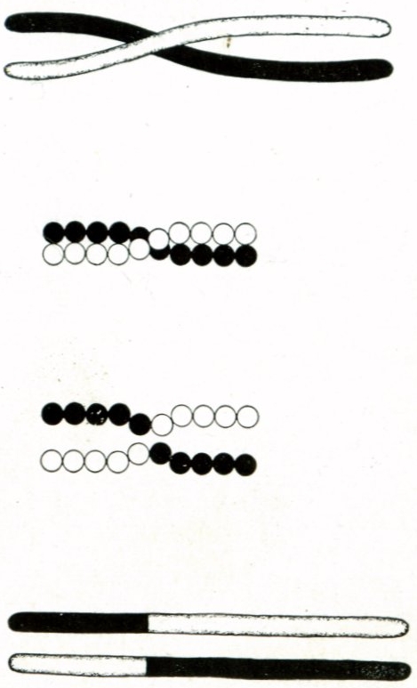
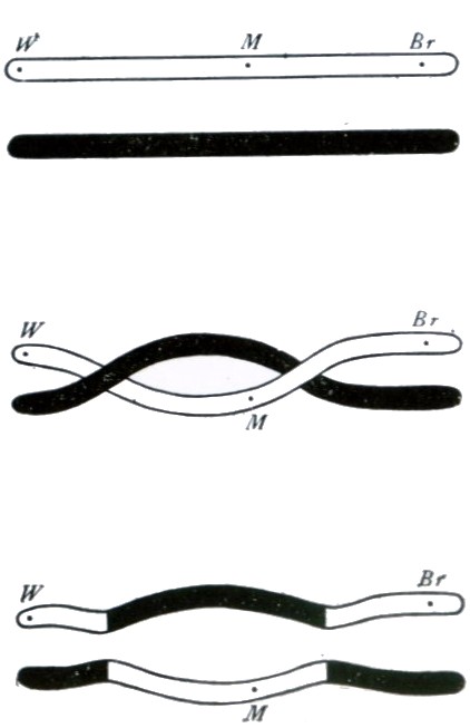
The combination operators we propose are all variants of crossover - a classic genetic programming technique rooted in the way a pair of DNA molecules exchanges genes during mitosis and meiosis, displayed on figure 1(a).
In DNA [38], as well as in most genetic programming literature [8, 9] the crossover operator combines 2 parent sequences to produce 2 children. In this section, in order to reduce complexity, we define the distributions as if only the first child program is saved and the second one is forgotten. Since program pair is equally likely to be selected for combination as (see eq. 19) this modification does not affect the resulting genetic developer distribution.
In one-point crossover a random cut position is selected and the trailing sections of 2 parent programs beginning with the cut point are swapped with each other. If the parent programs have different lengths, the cut point has to fit within both programs:
| (12) |
| (13) |
Hence the probability of being born out of one-point crossover is
| (14) |
Two-point crossover is similar, but instead of swapping the trailing ends of programs, a section in the middle of the programs is chosen, determined by randomly selected cut-off indices and and swapped:
| (15) |
Uniform crossover mirrors uniform mutation in that a loaded coin is tossed for each token in . With probability the token is replaced, but the replacement is not drawn randomly from the alphabet. Instead, the replacement comes from :
| (16) |
Finally, messy crossover is a version of one-point crossover without the assumption that both parent programs have to be cut at the same index . In messy crossover, one parent is cut at index , another is cut at index and the head of one is attached to the tail of the other:
| (17) |
3.5.3 Pruning operator
After initial experiments we found that generated programs often contain sections of unreachable code or code that makes changes to the execution state and fully reverses them. To address this, we introduced an additional operator for removing dead code (pruning): when Instant Scrum encounters a successful program, pruning helps separate sections of this program that led to its success from sections that appeared in a highly-rated program by accident.
Implementation of the pruning operator depends on the programming language at hand, here we define it as a pruning function that outputs a program functionally equivalent to (memory functions of are equal to that of ) and and a degenerate probability distribution:
| (18) |
3.5.4 Operator and parent selection
Let be a tuple of all available genetic operators, in order of introduction, i.e. and
Genetic developer’s program distribution is a mixture distribution, combining different operators that can be applied, weighted by learnable parameters, and different programs that can be sampled from the codebase, weighted by empirical quality (eq. 7).
| (19) |
This is a true probability distribution if and only if
3.5.5 Training the genetic developer
One challenge that remains to be solved to fully define the genetic developer (folowing section 3.2) is to define a learning from feedback strategy . To do this, we notice that equation 19 contains a multi-armed bandit [40] hiding in plain sight. Indeed, once the genetic developer samples and from the codebase, it has to pick one of 7 available options (pull one of 7 levers) to then receive a reward . This subproblem can be represented with a POMDP of its own and solved using one of the standard bandit algorithms [41].
Following Occam’s razor, we picked the simplest method, epsilon-greedy optimization: we calculate the value of each operator as mean total reward of programs generated with this operator:
| (20) |
where is the subset of the codebase produced via operator .
The procedure recalculates values and sets operator probabilities to
| (21) |
where is a hyperparameter responsible for regulating the exploration-exploitation tradeoff [42]
In future work, however, other bandit optimization algorithms can be used in its place 333Our open-source software implementation allows for drop-in replacement of bandit algorithms.
3.5.6 Hyperparameters
The genetic developer, as described above, has 2 hyperparameters:
-
1.
defines severity of mutation in and
-
2.
defines learnability of genetic operator distribution
Note that the team mechanism afforded by Instant Scrum can be used not only to combine genetic and neural program synthesis, but also to combine several genetic developers with different hyperparameters.
3.6 Neural developers
The neural developer, also known as the senior developer because of their unique ability to write original programs, is an LSTM [43] network followed by a linear layer that generates a sequence of vectors where and -th element of vector , , represents the probability of -th token of the program being -th token in the alphabet, . The last element of the vector represents a special end of program symbol. This vector depends deterministically on the full set of neural network parameters (LSTM and linear layer) and can be represented as a function . Then
| (22) |
For the procedure we use the algorithm proposed in [12]. The subproblem of generating a program is considered as a reinforcement learning episode of it’s own, where tokens are actions and token number (end of program token) is assigned reward . In this subenvironment is the policy network [44, chapter 13] trained using REINFORCE algorithm with Priority Queue Training. This algorithm involves a priority queue of best known programs: we implement it as programs from with highest which means that the neural developer can train on programs written by other developers.
can also represent several LSTM layers stacked or a different type of recurrent neural network, i.e. GRU [45]. Hyperparameters of this neural network, such as hidden state size and/or number of stacked layers are hyperparameters of the neural developer.
3.7 Dummy developer
The last developer we introduce is the simplest one:
| (23) |
Dummy developer does not generate novel programs. Instead, it uses the same quality-weighted program sampling as in equation 19 to decide which existing program to copy. Their utility may not be obvious at first, but note (section 3.3) that when the same program is added to the codebase several times, it’s total reward and quality estimates are averaged and grow more accurate.
Dummy developer is a smart compromise between speed at which Instant Scrum (algorithm 2) is searching the program space and the quality of it’s working map of the program space, focusing on its most "interesting" (high ) parts. Without dummy developer, all empirical total rewards would be low quality estimates of true fitness of the program and one spurious success of an otherwise bad program could steer the search in the wrong direction. On the other hand, we could test each program many times before adding it to the codebase, but that would slow down the search prohibitively.
4 Experimental setup
4.1 Teams
In the table below, we introduce 5 teams. Neural developers are denoted as lstm(hidden state dimensionality), several numbers mean a stacked LSTM. Genetic developers are denoted as , see secion 3.5.6. and are recommended configurations while , are ablation studies to prove that combination of neural and genetic methods is useful.
| Developer | ||||
| ✓ | ||||
| ✓ | ||||
| ✓ | ||||
| ✓ | ||||
| ✓ | ✓ | ✓ | ||
| ✓ | ||||
| ✓ | ||||
| ✓ | ||||
| ✓ | ||||
| ✓ | ||||
| dummy | ✓ | ✓ | ✓ | ✓ |
4.2 Language
Instant Scrum can be used to generate programs in any programming language provided:
-
1.
An interpreter , see section 2.1
-
2.
A known finite alphabet
-
3.
A pruning function
The complexity of the chosen language is important since in complex languages random perturbations of program source code often produce grammatically invalid programs. This issue has been addressed with structural models [46, 14] [9, chapter 4], however, we sidestep the issue entirely by using BF++ [39] - a simple language developed for programmatically interpretable reinforcement learning where most random combinations of characters are valid programs. Each BF++ command is represented with a single character, thus the only way to tokenize it is to let tokens be single characters.
4.3 Tasks
4.4 Initial populations
Where possible, we run all experiments twice - a control experiment with empty intial codebase, and an experiment where codebase is pre-populated with human-written programs from [39]. Exceptions to this rule are
-
•
Teams and that only have code modification (not generation) capability and thus require initialization
-
•
BipedalWalker-v2 environment, because no programs for this environment were provided in [39]
4.5 Stopping and scoring
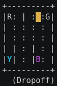
For Taxi we set an to sprints, meaning every developer in the team trains for 100000 iterations. For other tasks we used Exponential Variance Elimination [50] early stopping algorithm to stop the process when the positive trend in is not present for 10000 sprints. This approach rules out the hypothesis that Instant Scrum is equivalent to enumerative search and it finds good programs by exhaustion as opposed to learning - if that was the case, early stopping would fire immediately. Taxi environment is treated differently because programs that cannot pick up and drop off at least one passenger are always rewarded with -200 and at first it takes many iterations to synthesize at least one program that can. In addition to these stopping rules, a hard timelimit was set.
After the process is stopped, we pick 100 programs with the highest and make sure each of them has been tested at least 100 times, otherwise we run and add result to the codebase until 100 samples is reached.
4.6 Implementation
We implemented the framework with Python and Tensorflow as well as DEAP [51] for genetic operators. It is available at https://github.com/vadim0x60/cibi
5 Results
See table 1 for a summary of best programs generated. The metric used, average over 100 evaluations is the same metric that’s used in the OpenAI gym leaderboard, so we include the threshold required to join the leaderboard for context. Initial programs refers to the best program in the codebase before Instant Scrum starts when it is prepopulated with programs from [39].
The main hypothesis of this paper is confirmed: neurogenetic approach is superior to neural program induction or genetic programming separately. Besides, one unintuitive result of our experiments is that initialization of the codebase with previously available programs can be harmful, see . Overall, best results were acheived without inspiration from human experts, however, it is very valuable for lightweight teams with few small (in terms of ) developers.
Additionally, we can explore to see which of its many developers actually produced the best programs:
| Task | Init | Developer | |
| CartPole-v1 | 157.35 | lstm(256) | |
| CartPole-v1 | ✓ | 57.47 | lstm(256,256) |
| MountainCar | 91.65 | lstm(10,10) and pruning | |
| MountainCar | ✓ | 91.42 | lstm(50) |
| Taxi-v3 | -32.12 | lstm(50) | |
| Taxi-v3 | ✓ | -150.44 | human |
| BipedalWalker-v2 | 8.13 | lstm(256,256) |
The same is true for :
| Task | Init | Developer | |
| CartPole-v1 | 60.93 | lstm(50,50) | |
| CartPole-v1 | ✓ | 143.9 | lstm(50,50) |
| MountainCar | 92.53 | lstm(50,50) | |
| MountainCar | ✓ | 88.2 | lstm(50,50) |
| Taxi-v3 | -148.23 | , | |
| Taxi-v3 | ✓ | -150.44 | human |
| BipedalWalker-v2 | -0.15 | lstm(50,50) |
However, comparing results for versus proves that genetic developers have been intstrumental to the quality of these neural networks - this is to be expected with Priority Queue Training (see sec. 3.6).
6 Discussion
We have introduced a neurogenetic programming framework, demonstrated its efficacy and advantages over simpler program induction methods.
We believe that this framework can become a basis for many future methods - new methods of program synthesis can be built into the Instant Scrum framework as developers and combined with existing ones as necessary. In particular, one type of developer currently absent from our experiments is a neural mutation - a neural network that modifies existing programs and can be trained to modify them in a way that improves their performance. Another important direction is applying the framework to more specialized tasks like robotics or healthcare decision support.
Acknowledgements
This work was funded by the European Union’s Horizon 2020 research and innovation programme under grant agreement 812882. This work is part of "Personal Health Interfaces Leveraging HUman-MAchine Natural interactionS" (PhilHumans) project: https://www.philhumans.eu


| Environment | CartPole-v1 | MountainCarContinuous-v0 | Taxi-v3 | BipedalWalker-v2 | |||
| Initial programs | 20.48 | -6.55 | -150.44 | ||||
| 60.93 | 143.91 | 92.53 | 88.20 | -148.23 | -150.44 | -0.16 | |
| 157.35 | 57.47 | 91.65 | 91.42 | -32.12 | -150.44 | 8.13 | |
| - | 59.12 | - | 0 | - | -47.54 | - | |
| 71.38 | 96.64 | 88.41 | 91.38 | -198.9 | -150.44 | 6.17 | |
| Leaderboard threshold | 195 | 195 | 90 | 90 | 0 | 0 | 300 |
References
- Floreano et al. [2008] Dario Floreano, Peter Dürr, and Claudio Mattiussi. Neuroevolution: from architectures to learning. Evolutionary intelligence, 1(1):47–62, 2008.
- Li [2017] Yuxi Li. Deep reinforcement learning: An overview. arXiv preprint arXiv:1701.07274, 2017.
- Devlin et al. [2017a] Jacob Devlin, Rudy Bunel, Rishabh Singh, Matthew J. Hausknecht, and Pushmeet Kohli. Neural program meta-induction. CoRR, abs/1710.04157, 2017a. URL http://arxiv.org/abs/1710.04157.
- Garzon [2012] Max Garzon. Models of Massive Parallelism: Analysis of Cellular Automata and Neural Networks. Springer Publishing Company, Incorporated, 1st edition, 2012. ISBN 3642779077.
- Kolmogorov [1965] Andrei N Kolmogorov. Three approaches to the quantitative definition ofinformation’. Problems of information transmission, 1(1):1–7, 1965.
- Ptolemaeus et al. [1952] Claudius Ptolemaeus, Nicolaus Copernicus, Johannes Kepler, and Charles Glenn tr Wallis. The almagest. Encyclopaedia Britannica, 1952.
- Thorburn [1918] William M Thorburn. The myth of occam’s razor. Mind, 27(107):345–353, 1918.
- Banzhaf et al. [1998] Wolfgang Banzhaf, Peter Nordin, Robert E Keller, and Frank D Francone. Genetic programming: an introduction, volume 1. Morgan Kaufmann Publishers San Francisco, 1998.
- Koza [1992] John R Koza. Genetic programming: on the programming of computers by means of natural selection, volume 1. MIT press, 1992.
- Feng et al. [2020] Zhangyin Feng, Daya Guo, Duyu Tang, Nan Duan, Xiaocheng Feng, Ming Gong, Linjun Shou, Bing Qin, Ting Liu, Daxin Jiang, and Ming Zhou. Codebert: A pre-trained model for programming and natural languages, 2020.
- Devlin et al. [2018] Jacob Devlin, Ming-Wei Chang, Kenton Lee, and Kristina Toutanova. BERT: pre-training of deep bidirectional transformers for language understanding. CoRR, abs/1810.04805, 2018. URL http://arxiv.org/abs/1810.04805.
- Abolafia et al. [2018] Daniel A. Abolafia, Mohammad Norouzi, Jonathan Shen, Rui Zhao, and Quoc V. Le. Neural Program Synthesis with Priority Queue Training. arXiv preprint arXiv:1801.03526, 2018. URL http://arxiv.org/abs/1801.03526.
- Balog et al. [2016] Matej Balog, Alexander L. Gaunt, Marc Brockschmidt, Sebastian Nowozin, and Daniel Tarlow. Deepcoder: Learning to write programs. CoRR, abs/1611.01989, 2016. URL http://arxiv.org/abs/1611.01989.
- Alon et al. [2020] Uri Alon, Roy Sadaka, Omer Levy, and Eran Yahav. Structural language models of code. In International Conference on Machine Learning, pages 245–256. PMLR, 2020.
- [15] Algorithm synthesis: Deep learning and genetic programming. http://iao.hfuu.edu.cn/blogs/33-algorithm-synthesis-deep-learning-and-genetic-programming. (Accessed on 02/03/2021).
- Schwaber and Beedle [2002] Ken Schwaber and Mike Beedle. Agile software development with Scrum, volume 1. Prentice Hall Upper Saddle River, 2002.
- Livinskii et al. [2020] Vsevolod Livinskii, Dmitry Babokin, and John Regehr. Random testing for c and c++ compilers with yarpgen. Proc. ACM Program. Lang., 4(OOPSLA), November 2020. doi: 10.1145/3428264. URL https://doi.org/10.1145/3428264.
- Barany [2017] Gergö Barany. Liveness-driven random program generation. CoRR, abs/1709.04421, 2017. URL http://arxiv.org/abs/1709.04421.
- Polozov and Gulwani [2015] Oleksandr Polozov and Sumit Gulwani. Flashmeta: A framework for inductive program synthesis. In Proceedings of the 2015 ACM SIGPLAN International Conference on Object-Oriented Programming, Systems, Languages, and Applications, pages 107–126, 2015.
- Devlin et al. [2017b] Jacob Devlin, Jonathan Uesato, Surya Bhupatiraju, Rishabh Singh, Abdel-rahman Mohamed, and Pushmeet Kohli. Robustfill: Neural program learning under noisy i/o. In International conference on machine learning, pages 990–998. PMLR, 2017b.
- Le and Gulwani [2014] Vu Le and Sumit Gulwani. Flashextract: A framework for data extraction by examples. In Proceedings of the 35th ACM SIGPLAN Conference on Programming Language Design and Implementation, pages 542–553, 2014.
- Gulwani [2011] Sumit Gulwani. Automating string processing in spreadsheets using input-output examples. ACM Sigplan Notices, 46(1):317–330, 2011.
- Srivastava et al. [2010] Saurabh Srivastava, Sumit Gulwani, and Jeffrey S. Foster. From program verification to program synthesis. SIGPLAN Not., 45(1):313–326, January 2010. ISSN 0362-1340. doi: 10.1145/1707801.1706337. URL https://doi.org/10.1145/1707801.1706337.
- Ling et al. [2016] Wang Ling, Phil Blunsom, Edward Grefenstette, Karl Moritz Hermann, Tomáš Kočiskỳ, Fumin Wang, and Andrew Senior. Latent predictor networks for code generation. In Proceedings of the 54th Annual Meeting of the Association for Computational Linguistics (Volume 1: Long Papers), pages 599–609, 2016.
- Yin and Neubig [2017] Pengcheng Yin and Graham Neubig. A syntactic neural model for general-purpose code generation. In Proceedings of the 55th Annual Meeting of the Association for Computational Linguistics (Volume 1: Long Papers), pages 440–450, 2017.
- Rabinovich et al. [2017] Maxim Rabinovich, Mitchell Stern, and Dan Klein. Abstract syntax networks for code generation and semantic parsing. In Proceedings of the 55th Annual Meeting of the Association for Computational Linguistics (Volume 1: Long Papers), pages 1139–1149, 2017.
- Verma et al. [2018] Abhinav Verma, Vijayaraghavan Murali, Rishabh Singh, Pushmeet Kohli, and Swarat Chaudhuri. Programmatically interpretable reinforcement learning. In Jennifer Dy and Andreas Krause, editors, Proceedings of the 35th International Conference on Machine Learning, volume 80 of Proceedings of Machine Learning Research, pages 5045–5054, Stockholmsmässan, Stockholm Sweden, 10–15 Jul 2018. PMLR. URL http://proceedings.mlr.press/v80/verma18a.html.
- Kober et al. [2013] Jens Kober, J. Andrew Bagnell, and Jan Peters. Reinforcement learning in robotics: A survey. The International Journal of Robotics Research, 32(11):1238–1274, 2013. doi: 10.1177/0278364913495721. URL https://doi.org/10.1177/0278364913495721.
- [29] Vadim Liventsev. Heartpole: A transparent task for reinforcement learning in healthcare. https://github.com/vadim0x60/heartpole/blob/master/HeartPole_abstract.pdf. (Accessed on 01/31/2021).
- [30] Amirhossein Kiani, Tianli Ding, and Peter Henderson. Gymic: An openai gym environment for simulating sepsis treatment for icu patients. https://github.com/akiani/rlsepsis234/blob/master/writeup.pdf. (Accessed on 01/31/2021).
- Brockman et al. [2016] Greg Brockman, Vicki Cheung, Ludwig Pettersson, Jonas Schneider, John Schulman, Jie Tang, and Wojciech Zaremba. Openai gym, 2016.
- Åström [1965] K J Åström. Optimal control of Markov processes with incomplete state information. Journal of Mathematical Analysis and Applications, 10(1):174–205, 1965. ISSN 0022-247X. doi: https://doi.org/10.1016/0022-247X(65)90154-X. URL http://www.sciencedirect.com/science/article/pii/0022247X6590154X.
- Kramer [1964] Jr Kramer, J David R. Partially Observable Markov Processes., 1964.
- Brooks Jr [1995] Frederick P Brooks Jr. The mythical man-month: essays on software engineering. Pearson Education, 1995.
- Le Goues et al. [2012] Claire Le Goues, Michael Dewey-Vogt, Stephanie Forrest, and Westley Weimer. A systematic study of automated program repair: Fixing 55 out of 105 bugs for $8 each. In 2012 34th International Conference on Software Engineering (ICSE), pages 3–13. IEEE, 2012.
- Rückstiess et al. [2010] Thomas Rückstiess, Frank Sehnke, Tom Schaul, Daan Wierstra, Yi Sun, and Jürgen Schmidhuber. Exploring parameter space in reinforcement learning. Paladyn, 1(1):14–24, 2010.
- [37] Christopher R Devlin. Voting Systems: From Method to Algorithm. PhD thesis, California State University Channel Islands.
- Morgan [1916] Thomas Hunt Morgan. A Critique of the Theory of Evolution. Princeton University Press, 1916.
- Liventsev et al. [2021] Vadim Liventsev, Aki Härmä, and Milan Petković. Bf++:a language for general-purpose neural program synthesis, 2021.
- Robbins [1952] Herbert Robbins. Some aspects of the sequential design of experiments. Bulletin of the American Mathematical Society, 58(5):527–535, 1952.
- Kuleshov and Precup [2014] Volodymyr Kuleshov and Doina Precup. Algorithms for multi-armed bandit problems. CoRR, abs/1402.6028, 2014. URL http://arxiv.org/abs/1402.6028.
- Macready and Wolpert [1998] William G Macready and David H Wolpert. Bandit problems and the exploration/exploitation tradeoff. IEEE Transactions on evolutionary computation, 2(1):2–22, 1998.
- Gers et al. [1999] Felix A Gers, Jürgen Schmidhuber, and Fred Cummins. Learning to forget: Continual prediction with lstm. 1999.
- Sutton and Barto [2018] Richard S Sutton and Andrew G Barto. Reinforcement learning: An introduction. MIT press, 2018.
- Cho et al. [2014] Kyunghyun Cho, Bart Van Merriënboer, Caglar Gulcehre, Dzmitry Bahdanau, Fethi Bougares, Holger Schwenk, and Yoshua Bengio. Learning phrase representations using rnn encoder-decoder for statistical machine translation. arXiv preprint arXiv:1406.1078, 2014.
- [46] Peter A Whigham et al. Grammatically-based genetic programming.
- Barto et al. [1983] A. G. Barto, R. S. Sutton, and C. W. Anderson. Neuronlike adaptive elements that can solve difficult learning control problems. IEEE Transactions on Systems, Man, and Cybernetics, SMC-13(5):834–846, Sep. 1983. ISSN 2168-2909. doi: 10.1109/TSMC.1983.6313077.
- Moore [1990] Andrew William Moore. Efficient memory-based learning for robot control. Technical report, 1990.
- Dietterich [2000] Thomas G. Dietterich. Hierarchical reinforcement learning with the maxq value function decomposition. Journal of Artificial Intelligence Research, 13:227–303, 2000.
- [50] vadim0x60/evestop: Early stopping with exponential variance elmination. https://github.com/vadim0x60/evestop. (Accessed on 01/20/2021).
- Fortin et al. [2012] Félix-Antoine Fortin, François-Michel De Rainville, Marc-André Gardner, Marc Parizeau, and Christian Gagné. DEAP: Evolutionary algorithms made easy. Journal of Machine Learning Research, 13:2171–2175, jul 2012.