Numerical approximation and simulation of the stochastic wave equation on the sphere

Abstract.

Solutions to the stochastic wave equation on the unit sphere are approximated by spectral methods. Strong, weak, and almost sure convergence rates for the proposed numerical schemes are provided and shown to depend only on the smoothness of the driving noise and the initial conditions. Numerical experiments confirm the theoretical rates. The developed numerical method is extended to stochastic wave equations on higher-dimensional spheres and to the free stochastic Schrödinger equation on the unit sphere.

1. Introduction

The recent years have witnessed a strong interest in the theoretical study of (regularity) properties and the simulation of random fields, especially the ones that are defined by stochastic partial differential equations (SPDEs) on Euclidean spaces. This increase in the interest in random fields is due to the huge demand from applications as diverse as models for the motion of a strand of DNA floating in a fluid [12], climate and weather forecast models [17], models for the initiation and propagation of action potentials in neurons [15], random surface grow models [21], porous media and subsurface flow [7], or modeling of fibrosis in atrial tissue [9], for instance.

Yet, leaving the (by now well understood) Euclidean setting, theoretical results on random fields on Riemannian manifolds have just started to pop up in the literature. So far, this research has mostly focused on random fields on the sphere, e. g., [25, 26, 31, 29, 27, 30] and references therein. The interest of random fields on spheres is essentially driven by the fact that our planet Earth is approximately a sphere.

One example of an SPDE on the sphere and the main subject of the numerical analysis of this work is the stochastic wave equation

$$\partial_{tt}u(t)-\Delta_{\mathbb{S}^{2}}u(t)=\dot{W}(t),$$

driven by an isotropic $Q$-Wiener process. For details on the notation, see below. Besides the intrinsic mathematical interest, one motivation to study this equation comes from [6]. This work proposes and analyzes stochastic diffusion models for cosmic microwave background (CMB) radiation studies. Such models are given by damped wave equations on the sphere with random initial conditions. Since fluctuations in CMB observations may be generated by errors in the CMB map, contamination from the galaxy or distortions in the optics of the telescope [6], one may be interested in considering a driving noise living on the sphere.

Unfortunately, to this day, available and well-analyzed algorithms for an efficient simulation of random fields on manifolds do not match the current demand from applications. To name a few results from the literature on numerics for SPDEs on manifolds: the paper [29] proves rates of convergence for a spectral discretization of the heat equation on the sphere driven by an additive isotropic Gaussian noise; convergence rates of multilevel Monte Carlo finite and spectral element discretizations of stationary diffusion equations on the unit sphere with isotropic lognormal diffusion coefficients are considered in [19]; [8] proposes a simulation method for Gaussian fields defined over spheres cross time; a numerical approximation to solutions to random spherical hyperbolic diffusions is analyzed in [6]; rates of convergence of approximation schemes to solutions to fractional SPDEs on the unit sphere are shown in [2]; the work [22] studies a numerical scheme for simulating stochastic heat equations on the unit sphere with multiplicative noise; in [18] multilevel algorithms for the fast simulation of nonstationary Gaussian random fields on compact manifolds are analyzed. We are not aware of any results on numerical approximations of stochastic wave equations on manifolds.

In the present publication, we derive a representation of the infinite-dimensional analytical solution of the stochastic wave equation on the sphere driven by an isotropic $Q$-Wiener noise. This needs to be numerically approximated in order to be able to efficiently generate sample paths. The proposed algorithm is given by the truncation of a series expansion of the analytical solution, see (5). We prove strong and almost sure convergence rates of the fully discrete approximation scheme in Proposition 4.1. This is then used to show weak convergence results in Proposition 4.3 and Proposition 4.5. It turns out that these rates depend only on the decay of the angular power spectrum of the driving noise and the smoothness of the initial condition while they are independent of the chosen space and time grids. We show that depending on the smoothness of test functions, we obtain up to twice the strong order of convergence. These results are shown for the stochastic wave equation on the unit sphere $\mathbb{S}^{2}$ and then, strong and almost sure convergence results are extended to higher-dimensional spheres $\mathbb{S}^{d-1}$. Finally we obtain similar results for a related equation, namely the free stochastic Schrödinger equation on the sphere driven by an isotropic noise. Observe that the extension of our results to damped and nonlinear problems is not straightforward and needs further analysis. In particular, one would have to deal with additional errors in the space and time discretization.

A peculiarity in the present approach is that we are able to obtain two equations for the position and velocity component of the stochastic wave equation that can be simulated separately but with respect to two correlated driving noises. Therefore we put some focus on the properties of these correlated random fields and their simulation, see Proposition 3.1. With these in place we are able to show convergence of the position even when the series expansion of the velocity does not converge.

The outline of the paper is as follows: In Section 2 we recall definitions of isotropic Gaussian random fields on $\mathbb{S}^{2}$, of the Karhunen–Loève expansion in spherical harmonic functions of these fields from [31, 29], and of Wiener processes on the sphere. This then allows us to define the stochastic wave equation on the sphere in Section 3 and analyze its properties based on the semigroup approach. In Section 4 we approximate solutions to the SPDE with spectral methods. In addition, we provide convergence rates of these approximations in the $p$-th moment, in the $\mathbb{P}$-almost sure sense, and in the weak sense. Details on the numerical implementation of the studied discretizations are also presented in this section. Numerical illustrations of our theoretical findings are given in Section 5. Although the main focus of the paper is the stochastic wave equation on the unit sphere $\mathbb{S}^{2}$, we include two extensions in the last section that can be solved with the developed theory. Namely, an extension of the corresponding results to higher-dimensional spheres $\mathbb{S}^{d-1}\subset\mathbb{R}^{d}$ and an efficient algorithm for simulating the free stochastic Schrödinger equation on the sphere with its convergence properties.

2. Isotropic Gaussian random fields and Wiener processes on the sphere

We recall some notions and results, mostly from [29], in order to be able to define SPDEs on the sphere in the next section.

Throughout, we denote by $(\Omega,\mathcal{A},(\mathcal{F}_{t})_{t},\mathbb{P})$ a complete filtered probability space and write $\mathbb{S}^{2}$ for the unit sphere in $\mathbb{R}^{3}$, i. e.,

$$\mathbb{S}^{2}=\left\{x\in\mathbb{R}^{3},\|x\|_{\mathbb{R}^{3}}=1\right\},$$

where $\|\cdot\|_{\mathbb{R}^{3}}$ denotes the Euclidean norm. Let $(\mathbb{S}^{2},d)$ be the compact metric space with the geodesic metric given by

$$d(x,y)=\arccos\left(\langle x,y\rangle_{\mathbb{R}^{3}}\right)$$

for all $x,y\in\mathbb{S}^{2}$. We denote by $\mathcal{B}(\mathbb{S}^{2})$ the Borel $\sigma$-algebra of $\mathbb{S}^{2}$.

To introduce basis expansions often also called Karhunen–Loève expansions of a $Q$-Wiener process on the sphere, we first need to define spherical harmonic functions on $\mathbb{S}^{2}$. We recall that the Legendre polynomials $(P_{\ell},\ell\in\mathbb{N}_{0})$ are for example given by Rodrigues’ formula (see, e. g., [33])

$$P_{\ell}(\mu)=2^{-\ell}\frac{1}{\ell!}\,\frac{\partial^{\ell}}{\partial\mu^{\ell}}(\mu^{2}-1)^{\ell}$$

for all $\ell\in\mathbb{N}_{0}$ and $\mu\in[-1,1]$. These polynomials define the associated Legendre functions $(P_{\ell,m},\ell\in\mathbb{N}_{0},m=0,\ldots,\ell)$ by

$$P_{\ell,m}(\mu)=(-1)^{m}(1-\mu^{2})^{m/2}\frac{\partial^{m}}{\partial\mu^{m}}P_{\ell}(\mu)$$

for $\ell\in\mathbb{N}_{0}$, $m=0,\ldots,\ell$, and $\mu\in[-1,1]$. We further introduce the surface spherical harmonic functions $\mathcal{Y}=(Y_{\ell,m},\ell\in\mathbb{N}_{0},m=-\ell,\ldots,\ell)$ as mappings $Y_{\ell,m}\colon[0,\pi]\times[0,2\pi)\to\mathbb{C}$, which are given by

$$Y_{\ell,m}(\vartheta,\varphi)=\sqrt{\frac{2\ell+1}{4\pi}\frac{(\ell-m)!}{(\ell+m)!}}P_{\ell,m}(\cos\vartheta)\mathrm{e}^{\mathrm{i}m\varphi}$$

for $\ell\in\mathbb{N}_{0}$, $m=0,\ldots,\ell$, and $(\vartheta,\varphi)\in[0,\pi]\times[0,2\pi)$ and by

$$Y_{\ell,m}=(-1)^{m}\overline{Y_{\ell,-m}}$$

for $\ell\in\mathbb{N}$ and $m=-\ell,\ldots,-1$. It is well-known that the spherical harmonics form an orthonormal basis of $L^{2}(\mathbb{S}^{2})$, the subspace of real-valued functions in $L^{2}(\mathbb{S}^{2};\mathbb{C})$. In what follows we set for $y\in\mathbb{S}^{2}$

$$Y_{\ell,m}(y)=Y_{\ell,m}(\vartheta,\varphi),$$

where $y=(\sin\vartheta\cos\varphi,\sin\vartheta\sin\varphi,\cos\vartheta)$, i. e., we identify (with a slight abuse of notation) Cartesian and angular coordinates of the point $y\in\mathbb{S}^{2}$. Furthermore we denote by $\sigma$ the Lebesgue measure on the sphere which admits the representation

$$d\sigma(y)=\sin\vartheta\,d\vartheta\,d\varphi$$

for $y\in\mathbb{S}^{2}$, $y=(\sin\vartheta\cos\varphi,\sin\vartheta\sin\varphi,\cos\vartheta)$.

The spherical Laplacian, also called Laplace–Beltrami operator, is given in terms of spherical coordinates similarly to Section 3.4.3 in [31] by

$$\Delta_{\mathbb{S}^{2}}=(\sin\vartheta)^{-1}\frac{\partial}{\partial\vartheta}\left(\sin\vartheta\,\frac{\partial}{\partial\vartheta}\right)+(\sin\vartheta)^{-2}\frac{\partial^{2}}{\partial\varphi^{2}}.$$

It is well-known (see, e. g., Theorem 2.13 in [32]) that the spherical harmonic functions $\mathcal{Y}$ are the eigenfunctions of $\Delta_{\mathbb{S}^{2}}$ with eigenvalues $(-\ell(\ell+1),\ell\in\mathbb{N}_{0})$, i. e.,

$$\Delta_{\mathbb{S}^{2}}Y_{\ell,m}=-\ell(\ell+1)Y_{\ell,m}$$

for all $\ell\in\mathbb{N}_{0}$, $m=-\ell,\ldots,\ell$.

To characterize the regularity of solutions to SPDEs in what follows, we introduce the Sobolev space on $\mathbb{S}^{2}$ for a smoothness index $s\in\mathbb{R}$

$$H^{s}(\mathbb{S}^{2})=(\text{Id}-\Delta_{\mathbb{S}^{2}})^{-s/2}L^{2}(\mathbb{S}^{2})$$

together with its norm

$$\|f\|_{H^{s}(\mathbb{S}^{2})}=\|(\text{Id}-\Delta_{\mathbb{S}^{2}})^{s/2}f\|_{L^{2}(\mathbb{S}^{2})}$$

for some $f\in H^{s}(\mathbb{S}^{2})$ with $H^{0}(\mathbb{S}^{2})=L^{2}(\mathbb{S}^{2})$.

Furthermore, we work on $L^{p}(\Omega;H^{s}(\mathbb{S}^{2}))$ with norm

$$\|Z\|_{L^{p}(\Omega;H^{s}(\mathbb{S}^{2}))}=\operatorname{\mathbb{E}}\left[\|Z\|_{H^{s}(\mathbb{S}^{2})}^{p}\right]^{1/p}$$

for finite $p\geq 1$ and are now in place to introduce the following definitions:

A $\mathcal{A}\otimes\mathcal{B}(\mathbb{S}^{2})$-measurable mapping $Z\colon\Omega\times\mathbb{S}^{2}\rightarrow\mathbb{R}$ is called a real-valued random field on the unit sphere. Such a random field is called Gaussian if for all $k\in\mathbb{N}$ and $x_{1},\ldots,x_{k}\in\mathbb{S}^{2}$, the multivariate random variable $(Z(x_{1}),\ldots,Z(x_{k}))$ is multivariate Gaussian distributed. Finally, such a random field is called isotropic if its covariance function only depends on the distance $d(x,y)$, for $x,y\in\mathbb{S}^{2}$.

We recall Theorem 2.3 and Lemma 5.1 in [29] on the series expansions of isotropic Gaussian random fields on the sphere.

Lemma 2.1.

A centered, isotropic Gaussian random field $Z$ has a converging Karhunen–Loève expansion

$$Z=\sum_{\ell=0}^{\infty}\sum_{m=-\ell}^{\ell}a_{\ell,m}Y_{\ell,m}$$

with $a_{\ell,m}=(Z,Y_{\ell,m})_{L^{2}(\mathbb{S}^{2})}$ and $A_{\ell}=\operatorname{\mathbb{E}}[a_{\ell,m}\overline{a_{\ell,m}}]$ for all $m=-\ell,\ldots,\ell$, where $(A_{\ell},\ell\in\mathbb{N}_{0})$ is called the angular power spectrum of $Z$. For $\ell\in\mathbb{N}$, $m=1,\ldots,\ell$, and $\vartheta\in[0,\pi]$ set

$$L_{\ell,m}(\vartheta)=\sqrt{\frac{2\ell+1}{4\pi}\frac{(\ell-m)!}{(\ell+m)!}}P_{\ell,m}(\cos\vartheta).$$

Then for $y=(\sin\vartheta\cos\varphi,\sin\vartheta\sin\varphi,\cos\vartheta)$

$$Z(y)=\sum_{\ell=0}^{\infty}\left(\sqrt{A_{\ell}}X^{1}_{\ell,0}L_{\ell,0}(\vartheta)+\sqrt{2A_{\ell}}\sum_{m=1}^{\ell}L_{\ell,m}(\vartheta)(X^{1}_{\ell,m}\cos(m\varphi)+X^{2}_{\ell,m}\sin(m\varphi))\right)$$

in law, where $((X^{1}_{\ell,m},X^{2}_{\ell,m}),\ell\in\mathbb{N}_{0},m=0,\ldots,\ell)$ is a sequence of independent, real-valued, standard normally distributed random variables and $X^{2}_{\ell,0}=0$ for $\ell\in\mathbb{N}_{0}$.

In order to simulate solutions to the stochastic wave equation on the sphere, we need to approximate the driving noise which can be generated by a sequence of Gaussian random fields. We choose to truncate the above series expansion for an index $\kappa\in\mathbb{N}$ and set

$$Z^{\kappa}(y)=\sum_{\ell=0}^{\kappa}\left(\sqrt{A_{\ell}}X^{1}_{\ell,0}L_{\ell,0}(\vartheta)+\sqrt{2A_{\ell}}\sum_{m=1}^{\ell}L_{\ell,m}(\vartheta)(X^{1}_{\ell,m}\cos(m\varphi)+X^{2}_{\ell,m}\sin(m\varphi))\right),$$

where we recall $y=(\sin\vartheta\cos\varphi,\sin\vartheta\sin\varphi,\cos\vartheta)$ and $(\vartheta,\varphi)\in[0,\pi]\times[0,2\pi)$.

The above lemma then allows us to present the following results on $L^{p}(\Omega;L^{2}(\mathbb{S}^{2}))$ convergence and $\mathbb{P}$-almost sure convergence of the truncated series which are proven in Theorem 5.3 and Corollary 5.4 in [29].

Theorem 2.2.

Let the angular power spectrum $(A_{\ell},\ell\in\mathbb{N}_{0})$ of the centered, isotropic Gaussian random field $Z$ decay algebraically with order $\alpha>2$, i. e., there exist constants $C>0$ and $\ell_{0}\in\mathbb{N}$ such that $A_{\ell}\leq C\cdot\ell^{-\alpha}$ for all $\ell>\ell_{0}$. Then the series of approximate random fields $(Z^{\kappa},\kappa\in\mathbb{N})$ converges to the random field $Z$ in $L^{p}(\Omega;L^{2}(\mathbb{S}^{2}))$ for any finite $p\geq 1$, and the truncation error is bounded by

$$\|Z-Z^{\kappa}\|_{L^{p}(\Omega;L^{2}(\mathbb{S}^{2}))}\leq\hat{C}_{p}\cdot\kappa^{-(\alpha-2)/2}$$

for $\kappa>\ell_{0}$, where $\hat{C}_{p}$ is a constant depending on $p$, $C$, and $\alpha$.

In addition, $(Z^{\kappa},\kappa\in\mathbb{N})$ converges $\mathbb{P}$-almost surely and for all $\delta<(\alpha-2)/2$, the truncation error is asymptotically bounded by

$$\|Z-Z^{\kappa}\|_{L^{2}(\mathbb{S}^{2})}\leq\kappa^{-\delta},\quad\mathbb{P}\text{-a.s.}.$$

We follow [29], where isotropic Gaussian random fields are connected to $Q$-Wiener processes. There it is shown that an isotropic $Q$-Wiener process $(W(t),t\in\mathbb{T})$ on some finite time interval $\mathbb{T}=[0,T]$ with values in $L^{2}(\mathbb{S}^{2})$ can be represented by the expansion

(1) $$\begin{split}W(t,y)&=\sum_{\ell=0}^{\infty}\sum_{m=-\ell}^{\ell}a^{\ell,m}(t)Y_{\ell,m}(y)\\ &=\sum_{\ell=0}^{\infty}\left(\sqrt{A_{\ell}}\beta_{1}^{\ell,0}(t)Y_{\ell,0}(y)+\sqrt{2A_{\ell}}\sum_{m=1}^{\ell}(\beta_{1}^{\ell,m}(t)\operatorname{Re}Y_{\ell,m}(y)+\beta_{2}^{\ell,m}(t)\operatorname{Im}Y_{\ell,m}(y))\right)\\ &=\sum_{\ell=0}^{\infty}\left(\sqrt{A_{\ell}}\beta_{1}^{\ell,0}(t)L_{\ell,0}(\vartheta)+\sqrt{2A_{\ell}}\sum_{m=1}^{\ell}L_{\ell,m}(\vartheta)(\beta_{1}^{\ell,m}(t)\cos(m\varphi)+\beta_{2}^{\ell,m}(t)\sin(m\varphi))\right),\end{split}$$

where $((\beta_{1}^{\ell,m},\beta_{2}^{\ell,m}),\ell\in\mathbb{N}_{0},m=0,\ldots,\ell)$ is a sequence of independent, real-valued Brownian motions with $\beta_{2}^{\ell,0}=0$ for $\ell\in\mathbb{N}_{0}$ and $t\in\mathbb{T}$. The covariance operator $Q$ is characterized similarly to the introduction in [28] by

$$QY_{\ell,m} =A_{\ell}Y_{\ell,m}$$

for $\ell\in\mathbb{N}_{0}$ and $m=-\ell,\ldots,\ell$, i. e., the eigenvalues of $Q$ are given by the angular power spectrum $(A_{\ell},\ell\in\mathbb{N}_{0})$, and the eigenfunctions are the spherical harmonic functions.

Due to the properties of Brownian motion, the above $Q$-Wiener process can be generated by increments which are isotropic Gaussian random fields with angular power spectrum $(hA_{\ell},\ell\in\mathbb{N}_{0})$ for a time step size $h$.

3. The stochastic wave equation on the sphere

With the preparations from the preceding section at hand, we have all necessary tools to introduce the main subject of our study.

The stochastic wave equation on the sphere is defined as

(2) $$\partial_{tt}u(t)-\Delta_{\mathbb{S}^{2}}u(t)=\dot{W}(t)$$

with initial conditions $u(0)=v_{1}\in L^{2}(\Omega;L^{2}(\mathbb{S}^{2}))$ and $\partial_{t}u(0)=v_{2}\in L^{2}(\Omega;L^{2}(\mathbb{S}^{2}))$, where $t\in\mathbb{T}=[0,T]$, $T<+\infty$. For ease of presentation, we consider the case of non-random initial conditions. The case of random initial conditions follows under appropriate integrability assumptions. The notation $\dot{W}$ stands for the formal derivative of the $Q$-Wiener process with series expansion (1) as introduced in Section 2.

Denoting the velocity of the solution by $u_{2}=\partial_{t}u_{1}=\partial_{t}u$, one can rewrite (2) as

$$\mathop{}\!\mathrm{d}X(t) =AX(t)\,\mathop{}\!\mathrm{d}t+G\,\mathop{}\!\mathrm{d}W(t)$$

(3) $$X(0) =X_{0},$$

where

$$A=\begin{pmatrix}0&I\\ \Delta_{\mathbb{S}^{2}}&0\end{pmatrix},\quad G=\begin{pmatrix}0\\ I\end{pmatrix},\quad X=\begin{pmatrix}u_{1}\\ u_{2}\end{pmatrix},\quad X_{0}=\begin{pmatrix}v_{1}\\ v_{2}\end{pmatrix}.$$

Existence of a unique mild solution of the abstract formulation (3) of the stochastic wave equation on the sphere follows from classical results on linear SPDEs, see for instance [11], and this mild solution reads

$$X(t)=\mathrm{e}^{tA}X_{0}+\int_{0}^{t}\mathrm{e}^{(t-s)A}G\,\mathop{}\!\mathrm{d}W(s).$$

Equivalently, the integral formulation of our problem is given by

(4) $$\begin{cases}u_{1}(t)&\displaystyle=v_{1}+\int_{0}^{t}u_{2}(s)\,\mathop{}\!\mathrm{d}s\\ u_{2}(t)&\displaystyle=v_{2}+\int_{0}^{t}\Delta_{\mathbb{S}^{2}}u_{1}(s)\,\mathop{}\!\mathrm{d}s+W(t).\end{cases}$$

Since the spherical harmonic functions $\mathcal{Y}=(Y_{\ell,m},\ell\in\mathbb{N}_{0},m=-\ell,\ldots,\ell)$ form an orthonormal basis of $L^{2}(\mathbb{S}^{2})$ and are eigenfunctions of $\Delta_{\mathbb{S}^{2}}$, we insert the following ansatz for a series expansion of the exact solution to SPDE (2)

(5) $$u_{1}(t)=\displaystyle\sum_{\ell=0}^{\infty}\sum_{m=-\ell}^{\ell}u_{1}^{\ell,m}(t)Y_{\ell,m}\quad\text{and}\quad u_{2}(t)=\displaystyle\sum_{\ell=0}^{\infty}\sum_{m=-\ell}^{\ell}u_{2}^{\ell,m}(t)Y_{\ell,m}$$

into equation (4) and compare the coefficients in front of $Y_{\ell,m}$ to obtain the following system

$$u_{1}^{\ell,m}(t) =v_{1}^{\ell,m}+\int_{0}^{t}u_{2}^{\ell,m}(s)\,\mathop{}\!\mathrm{d}s$$

$$u_{2}^{\ell,m}(t) =v_{2}^{\ell,m}-\ell(\ell+1)\int_{0}^{t}u_{1}^{\ell,m}(s)\,\mathop{}\!\mathrm{d}s+a^{\ell,m}(t),$$

where $v_{1}^{\ell,m}$, $v_{2}^{\ell,m}$, resp. $a^{\ell,m}$ are the coefficients of the expansions of the initial values $v_{1}$ and $v_{2}$, resp. weighted Brownian motions in the expansion of the noise (1).

Writing the evolution of the initial values in the above linear harmonic oscillators with rotation matrices and using the variation of constants formula, one derives the following system for the coefficients of the expansions of the solution

(6) $$\begin{cases}u_{1}^{\ell,m}(t)&\displaystyle=\cos(t(\ell(\ell+1))^{1/2})v_{1}^{\ell,m}+(\ell(\ell+1))^{-1/2}\sin(t(\ell(\ell+1))^{1/2})v_{2}^{\ell,m}+\hat{W}_{1}^{\ell,m}(t)\\ u_{2}^{\ell,m}(t)&\displaystyle=-(\ell(\ell+1))^{1/2}\sin(t(\ell(\ell+1))^{1/2})v_{1}^{\ell,m}+\cos(t(\ell(\ell+1))^{1/2})v_{2}^{\ell,m}+\hat{W}_{2}^{\ell,m}(t),\end{cases}$$

where

$$\hat{W}^{\ell,m}(t)=\begin{pmatrix}\hat{W}_{1}^{\ell,m}(t)\\ \hat{W}_{2}^{\ell,m}(t)\end{pmatrix}=\displaystyle\int_{0}^{t}R^{\ell}(t-s)\,\mathop{}\!\mathrm{d}a^{\ell,m}(s)$$

with

$$R^{\ell}(t)=\begin{pmatrix}R^{\ell}_{1}(t)\\ R^{\ell}_{2}(t)\end{pmatrix}=\begin{pmatrix}(\ell(\ell+1))^{-1/2}\sin(t(\ell(\ell+1))^{1/2})\\ \cos(t(\ell(\ell+1))^{1/2})\end{pmatrix}$$

for $\ell\neq 0$ and

$$\hat{W}^{0,0}(t)=\begin{pmatrix}\hat{W}_{1}^{0,0}(t)\\ \hat{W}_{2}^{0,0}(t)\end{pmatrix}=\begin{pmatrix}\displaystyle\int_{0}^{t}a^{0,0}(s)\,\mathop{}\!\mathrm{d}s\\ a^{0,0}(t)\end{pmatrix}.$$

We now characterize the above stochastic convolutions $\hat{W}_{i}^{\ell,m}$ for $i=1,2$.

Proposition 3.1.

The stochastic convolution $\hat{W}(t)$ is Gaussian with mean zero and expansion

$$\hat{W}(t,y) =\sum_{\ell=0}^{\infty}\sum_{m=-\ell}^{\ell}W^{\ell,m}(t)Y_{\ell,m}(y)$$

$$=\sum_{\ell=0}^{\infty}\left(\sqrt{A_{\ell}}\hat{\beta}_{1}^{\ell,0}(t)Y_{\ell,0}(y)+\sqrt{2A_{\ell}}\sum_{m=1}^{\ell}(\hat{\beta}_{1}^{\ell,m}(t)\operatorname{Re}Y_{\ell,m}(y)+\hat{\beta}_{2}^{\ell,m}(t)\operatorname{Im}Y_{\ell,m}(y))\right)$$

$$=\sum_{\ell=0}^{\infty}\left(\sqrt{A_{\ell}}\hat{\beta}_{1}^{\ell,0}(t)L_{\ell,0}(\vartheta)+\sqrt{2A_{\ell}}\sum_{m=1}^{\ell}L_{\ell,m}(\vartheta)(\hat{\beta}_{1}^{\ell,m}(t)\cos(m\varphi)+\hat{\beta}_{2}^{\ell,m}(t)\sin(m\varphi))\right),$$

where equality is in distribution.

The processes $(\hat{\beta}^{\ell,m}_{i}(t),i=1,2,\ell\in\mathbb{N}_{0},m=-\ell,\ldots,\ell)$ are given by

$$\hat{\beta}^{\ell,m}_{i}(t)=\begin{pmatrix}\beta_{i,1}^{\ell,m}(t)\\ \beta_{i,2}^{\ell,m}(t)\end{pmatrix}=D_{\ell}(t)X^{\ell,m}_{i}$$

for a sequence $(X^{\ell,m}_{i}=(X_{i,1}^{\ell,m},X_{i,2}^{\ell,m})^{T},i=1,2,\ell\in\mathbb{N}_{0},m=-\ell,\ldots,\ell)$ of independent, identically distributed random variables with $X^{\ell,m}_{i,j}\sim\mathcal{N}(0,1)$. The term $D_{\ell}(t)$ denotes the Cholesky decomposition of the covariance matrix $C_{\ell}(t)$ of $\hat{W}^{\ell,m}(t)$. More specifically, $D_{\ell}$ satisfies

$$D_{\ell}(t)D_{\ell}(t)^{T}=C_{\ell}(t)$$

with

$$C_{\ell}(t)=\begin{pmatrix}\frac{2(\ell(\ell+1))^{1/2}t-\sin(2(\ell(\ell+1))^{1/2}t)}{4(\ell(\ell+1))^{3/2}}&\frac{\sin((\ell(\ell+1))^{1/2}t)^{2}}{2(\ell(\ell+1))}\\ \frac{\sin((\ell(\ell+1))^{1/2}t)^{2}}{2(\ell(\ell+1))}&\frac{2(\ell(\ell+1))^{1/2}t+\sin(2(\ell(\ell+1))^{1/2}t)}{4(\ell(\ell+1))^{1/2}}\end{pmatrix}$$

for $\ell\neq 0$ and

$$C_{0}(t)=\begin{pmatrix}t^{3}/3&t^{2}/2\\ t^{2}/2&t\end{pmatrix}.$$

Proof.

We observe first that $\hat{W}(t)$ satisfies by (1)

$$\hat{W}(t) =\sum_{\ell=0}^{\infty}\sum_{m=-\ell}^{\ell}\hat{W}^{\ell,m}(t)Y_{\ell,m}$$

$$=\hat{W}^{0,0}(t)Y_{0,0}+\sum_{\ell=1}^{\infty}\sum_{m=-\ell}^{\ell}\int_{0}^{t}R^{\ell}(t-s)\,\mathop{}\!\mathrm{d}a^{\ell,m}(s)Y_{\ell,m}$$

$$=\hat{W}^{0,0}(t)Y_{0,0}+\sum_{\ell=1}^{\infty}\sqrt{A_{\ell}}\left[\int_{0}^{t}R^{\ell}(t-s)\,\mathop{}\!\mathrm{d}\beta_{1}^{\ell,0}(s)Y_{\ell,0}\right.$$

$$\left.\hskip 50.00008pt+\sqrt{2}\sum_{m=1}^{\ell}\left(\int_{0}^{t}R^{\ell}(t-s)\,\mathop{}\!\mathrm{d}\beta_{1}^{\ell,m}(s)\operatorname{Re}Y_{\ell,m}+\int_{0}^{t}R^{\ell}(t-s)\,\mathop{}\!\mathrm{d}\beta_{2}^{\ell,m}(s)\operatorname{Im}Y_{\ell,m}\right)\right]$$

with independent Brownian motions $(\beta_{1}^{\ell,m},\ell\in\mathbb{N}_{0},m=0,\ldots,\ell)$ and $(\beta_{2}^{\ell,m},\ell\in\mathbb{N},m=1,\ldots,\ell)$. Since all Brownian motions are centered and independent, it is sufficient to compute the following covariances which are given by

$$C_{0}(t) =A_{0}^{-1}\begin{pmatrix}\operatorname{\mathbb{E}}[\hat{W}^{0,0}_{1}(t)^{2}]&\operatorname{\mathbb{E}}[\hat{W}_{1}^{0,0}(t)\hat{W}_{2}^{0,0}(t)]\\ \operatorname{\mathbb{E}}[\hat{W}_{1}^{0,0}(t)\hat{W}_{2}^{0,0}(t)]&\operatorname{\mathbb{E}}[\hat{W}_{2}^{0,0}(t)^{2}]\end{pmatrix}$$

$$=A_{0}^{-1}\begin{pmatrix}\operatorname{\mathbb{E}}[(\int_{0}^{t}a^{0,0}(s)\,\mathop{}\!\mathrm{d}s)^{2}]&\operatorname{\mathbb{E}}[\int_{0}^{t}a^{0,0}(s)a^{0,0}(t)\,\mathop{}\!\mathrm{d}s]\\ \operatorname{\mathbb{E}}[\int_{0}^{t}a^{0,0}(s)a^{0,0}(t)\,\mathop{}\!\mathrm{d}s]&\operatorname{\mathbb{E}}[(a^{0,0}(t))^{2}]\end{pmatrix}=\begin{pmatrix}t^{3}/3&t^{2}/2\\ t^{2}/2&t\end{pmatrix}$$

for $\ell=0$ and else for $i=1,2$

$$C_{\ell}(t) =\begin{pmatrix}\operatorname{\mathbb{E}}[(\text{Int}_{1})^{2}]&\operatorname{\mathbb{E}}[\text{Int}_{1}\text{Int}_{2}]\\ \operatorname{\mathbb{E}}[\text{Int}_{1}\text{Int}_{2}]&\operatorname{\mathbb{E}}[(\text{Int}_{2})^{2}]\end{pmatrix}$$

$$=\begin{pmatrix}\int_{0}^{t}R^{\ell}_{1}(t-s)^{2}\,\mathop{}\!\mathrm{d}s&\int_{0}^{t}R^{\ell}_{1}(t-s)R^{\ell}_{2}(t-s)\,\mathop{}\!\mathrm{d}s\\ \int_{0}^{t}R^{\ell}_{1}(t-s)R^{\ell}_{2}(t-s)\,\mathop{}\!\mathrm{d}s&\int_{0}^{t}R^{\ell}_{2}(t-s)^{2}\,\mathop{}\!\mathrm{d}s\end{pmatrix}$$

$$=\begin{pmatrix}\frac{2(\ell(\ell+1))^{1/2}t-\sin(2(\ell(\ell+1))^{1/2}t)}{4(\ell(\ell+1))^{3/2}}&\frac{\sin((\ell(\ell+1))^{1/2}t)^{2}}{2(\ell(\ell+1))}\\ \frac{\sin((\ell(\ell+1))^{1/2}t)^{2}}{2(\ell(\ell+1))}&\frac{2(\ell(\ell+1))^{1/2}t+\sin(2(\ell(\ell+1))^{1/2}t)}{4(\ell(\ell+1))^{1/2}}\end{pmatrix},$$

where we have set $\text{Int}_{1}=\int_{0}^{t}R^{\ell}_{1}(t-s)\,\mathop{}\!\mathrm{d}\beta_{i}^{\ell,m}(s)$ and $\text{Int}_{2}=\int_{0}^{t}R^{\ell}_{2}(t-s)\,\mathop{}\!\mathrm{d}\beta_{i}^{\ell,m}(s)$.

Setting $D_{\ell}(t)$ the Cholesky decomposition of the above covariance matrices satisfying

$$D_{\ell}(t)^{T}D_{\ell}(t)=C_{\ell}(t)$$

we obtain for $\ell\neq 0$ and $i=1,2$ that

$$D_{\ell}(t)X^{\ell,m}_{i}=\int_{0}^{t}R^{\ell}(t-s)\,\mathop{}\!\mathrm{d}\beta_{i}^{\ell,m}(s)$$

in distribution and similarly for $\ell=0$

$$D_{\ell}(t)X^{\ell,m}_{1}=\hat{W}^{0,0}(t)$$

with $(X^{\ell,m}_{i}=(X_{i,1}^{\ell,m},X_{i,2}^{\ell,m})^{T},i=1,2,\ell\in\mathbb{N}_{0},m=-\ell,\ldots,\ell)$ independent and identically distributed standard normally distributed random variables. This concludes the proof. ∎

Remark 3.2.

Since we are interested in the simulation of sample paths of solutions to (3), we need to generate increments of $\hat{W}^{\ell,m}(t)$. Therefore it is important to observe that

$$\hat{\beta}^{\ell,m}_{i}(t)-\hat{\beta}^{\ell,m}_{i}(s)=D_{\ell}(t-s)X^{\ell,m}_{i}$$

in distribution for $s<t$. In this way we can generate sample paths of $\hat{W}(t)$ by sums of independent Gaussian increments.

For completeness we also remark that the Cholesky decomposition $D_{\ell}(t)$ can be computed explicitly and is given by

(7) $$D_{\ell}(t)=\begin{pmatrix}d_{1,1}&d_{1,2}\\ 0&d_{2,2}\end{pmatrix}$$

with

$$d_{1,1} =\frac{(2(\ell(\ell+1))^{1/2}t-\sin(2(\ell(\ell+1))^{1/2}t))^{1/2}}{2(\ell(\ell+1))^{3/4}}$$

$$d_{1,2} =\frac{\sin((\ell(\ell+1))^{1/2}t)^{2}}{(\ell(\ell+1))^{1/4}(2(\ell(\ell+1))^{1/2}t-\sin(2(\ell(\ell+1))^{1/2}t))^{1/2}}$$

$$d_{2,2} =\left(\frac{4(\ell(\ell+1))t^{2}-\sin(2(\ell(\ell+1))^{1/2}t)^{2}-4\sin((\ell(\ell+1))^{1/2}t)^{4}}{4(\ell(\ell+1))^{1/2}(2(\ell(\ell+1))^{1/2}t-\sin(2(\ell(\ell+1))^{1/2}t))}\right)^{1/2}$$

for $\ell\neq 0$ and

$$D_{0}(t)=t^{1/2}\begin{pmatrix}t/\sqrt{3}&\sqrt{3}/2\\ 0&1/2\end{pmatrix}.$$

We close this section by showing regularity estimates for the solution of (2) that depend on the regularity of the initial conditions and the driving noise. These properties allow to obtain optimal weak convergence rates in Section 4.

Proposition 3.3.

Denote by $X=(u_{1},u_{2})$ the solution to the stochastic wave equation (3) with initial value $(v_{1},v_{2})$. Assume that there exist $\ell_{0}\in\mathbb{N}$, $\alpha>2$, and a constant $C>0$ such that the angular power spectrum of the driving noise $(A_{\ell},\ell\in\mathbb{N}_{0})$ satisfies $A_{\ell}\leq C\cdot\ell^{-\alpha}$ for all $\ell>\ell_{0}$. Then, for all $t\in[0,T]$, $m\in\mathbb{N}$, and $s<\alpha/2$ with $v_{1}\in H^{s}(\mathbb{S}^{2})$ and $v_{2}\in H^{s-1}(\mathbb{S}^{2})$, $u_{1}(t)\in L^{2m}(\Omega;H^{s}(\mathbb{S}^{2}))$, i. e., there exists a constant $M$ such that

$$\|u_{1}(t)\|_{L^{2m}(\Omega;H^{s}(\mathbb{S}^{2}))}\leq M(1+\|v_{1}\|_{H^{s}(\mathbb{S}^{2})}+\|v_{2}\|_{H^{s-1}(\mathbb{S}^{2})})<+\infty.$$

And for all $t\in[0,T]$, $m\in\mathbb{N}$, and $s<\alpha/2-1$ with $v_{1}\in H^{s+1}(\mathbb{S}^{2})$ and $v_{2}\in H^{s}(\mathbb{S}^{2})$, $u_{2}(t)\in L^{2m}(\Omega;H^{s}(\mathbb{S}^{2}))$, i. e., there exists a constant $M$ such that

$$\|u_{2}(t)\|_{L^{2m}(\Omega;H^{s}(\mathbb{S}^{2}))}\leq M(1+\|v_{1}\|_{H^{s+1}(\mathbb{S}^{2})}+\|v_{2}\|_{H^{s}(\mathbb{S}^{2})})<+\infty.$$

Proof.

Let us first observe that

$$\|u_{1}(t)\|_{L^{2m}(\Omega;H^{s}(\mathbb{S}^{2}))}$$

$$\hskip 30.00005pt\leq\left\|\sum_{\ell=0}^{\infty}\sum_{m=-\ell}^{\ell}\left(R^{\ell}_{2}(t)v_{1}^{\ell,m}+R^{\ell}_{1}(t)v_{2}^{\ell,m}\right)Y_{\ell,m}\right\|_{L^{2m}(\Omega;H^{s}(\mathbb{S}^{2}))}+\left\|\hat{W}(t)\right\|_{L^{2m}(\Omega;H^{s}(\mathbb{S}^{2}))}.$$

The first term with respect to the initial conditions satisfies

$$\left\|\sum_{\ell=1}^{\infty}\sum_{m=-\ell}^{\ell}\left(R^{\ell}_{2}(t)v_{1}^{\ell,m}+R^{\ell}_{1}(t)v_{2}^{\ell,m}\right)Y_{\ell,m}\right\|_{H^{s}(\mathbb{S}^{2})}^{2}$$

$$\qquad\leq 2\sum_{\ell=1}^{\infty}\sum_{m=-\ell}^{\ell}\left((1+\ell(\ell+1))^{s}|v_{1}^{\ell,m}|^{2}+(1+\ell(\ell+1))^{s}(\ell(\ell+1))^{-1}|v_{2}^{\ell,m}|^{2}\right)$$

$$\qquad\leq C(\|v_{1}\|_{H^{s}(\mathbb{S}^{2})}^{2}+\|v_{2}\|_{H^{s-1}(\mathbb{S}^{2})}^{2}).$$

Given the angular power spectrum of $\hat{W}(t)$ in Proposition 3.1, it follows for the second moment, i. e. $m=1$, that

$$\left\|\hat{W}(t)\right\|_{L^{2}(\Omega;H^{s}(\mathbb{S}^{2}))}^{2} =\left\|(\text{Id}-\Delta_{\mathbb{S}^{2}})^{s/2}\hat{W}(t)\right\|_{L^{2}(\Omega;L^{2}(\mathbb{S}^{2}))}^{2}$$

$$=\sum_{\ell=0}^{\infty}(2\ell+1)(1+\ell(\ell+1))^{s}\frac{2(\ell(\ell+1))^{1/2}t-\sin(2(\ell(\ell+1))^{1/2}t)}{4(\ell(\ell+1))^{3/2}}A_{\ell},$$

which converges for $\alpha>2s$ since the elements of the sum behave like $\ell^{2s-\alpha-1}$. By Fernique’s theorem [14], this convergence implies that the norm is finite for all $m$ and arbitrary moment bounds can for example be obtained by the Burkholder–Davis–Gundy inequality.

Similar computations for $u_{2}$ conclude the proof. ∎

4. Convergence analysis

In this section, we numerically solve the wave equation on the sphere driven by additive $Q$-Wiener noise with spectral methods. We approximate the solution by truncation of the derived spectral representation and show convergence rates in $p$-th moment, $\mathbb{P}$-almost surely, and in the weak sense.

An efficient simulation of numerical approximations to solutions to the stochastic wave equation on the sphere (2) is then obtained via Algorithm 1.

Algorithm 1 Simulations of paths of the solution to (2)

1:  Fix a truncation index $\kappa\in\mathbb{N}$.

2:  Compute a discrete time grid $0=t_{0}<t_{1}<\ldots<t_{n}=T$, $n\in\mathbb{N}$, with time step $h$.

3:  Compute the covariance matrix $C_{\ell}(h)$ of the stochastic integrals $\hat{W}_{1}^{\ell,m}(h)$ and $\hat{W}_{2}^{\ell,m}(h)$ in Proposition 3.1.

4:  Perform a Cholesky decomposition of $C_{\ell}(h)=D_{\ell}(h)^{T}D_{\ell}(h)$ or use the explicit formula (7).

5:  Use $D_{\ell}(h)$ to generate noise increments

$$\hat{W}^{\ell,m}(h)=\begin{pmatrix}\hat{W}_{1}^{\ell,m}(h)\\ \hat{W}_{2}^{\ell,m}(h)\end{pmatrix}=D_{\ell}\begin{pmatrix}\beta_{1}^{\ell,m}(h)\\ \beta_{2}^{\ell,m}(h)\end{pmatrix}\sqrt{A_{\ell}}.$$

6:  Compute $u_{1}^{\ell,m}(t_{j}+h)$ and $u_{2}^{\ell,m}(t_{j}+h)$ recursively using (6)

$$u^{\ell,m}(t_{j+1})=\begin{pmatrix}R_{2}^{\ell}(h)\\ -\ell(\ell+1)R_{1}^{\ell}(h)\end{pmatrix}u_{1}^{\ell,m}(t_{j})+R^{\ell}(h)u_{2}^{\ell,m}(t_{j})+\hat{W}^{\ell,m}(h).$$

7:  Truncate the ansatz (5) at the fixed positive integer $\kappa$ to get the numerical approximations

(8) $$u_{1}^{\kappa}(t_{j})=\displaystyle\sum_{\ell=0}^{\kappa}\sum_{m=-\ell}^{\ell}u_{1}^{\ell,m}(t_{j})Y_{\ell,m}\quad\text{and}\quad u_{2}^{\kappa}(t_{j})=\displaystyle\sum_{\ell=0}^{\kappa}\sum_{m=-\ell}^{\ell}u_{2}^{\ell,m}(t_{j})Y_{\ell,m}.$$

The strong errors of this truncation procedure are given in the following proposition.

Proposition 4.1.

Let $t\in\mathbb{T}$ and $0=t_{0}<\cdots<t_{n}=t$ be a discrete time partition for $n\in\mathbb{N}$, which yields a recursive representation of the solution $X=(u_{1},u_{2})$ of the stochastic wave equation on the sphere (3) given by (5). Assume that the initial values satisfy $v_{1}\in H^{\beta}(\mathbb{S}^{2})$ and $v_{2}\in H^{\gamma}(\mathbb{S}^{2})$. Furthermore, assume that there exist $\ell_{0}\in\mathbb{N}$, $\alpha>2$, and a constant $C>0$ such that the angular power spectrum of the driving noise $(A_{\ell},\ell\in\mathbb{N}_{0})$ satisfies $A_{\ell}\leq C\cdot\ell^{-\alpha}$ for all $\ell>\ell_{0}$. Then, the error of the approximate solution $X^{\kappa}=(u_{1}^{\kappa},u_{2}^{\kappa})$, given by (8), is bounded uniformly in time and independently of the time discretization by

$$\|u_{1}(t)-u_{1}^{\kappa}(t)\|_{L^{p}(\Omega;L^{2}(\mathbb{S}^{2}))} \leq\hat{C}_{p}\cdot\left(\kappa^{-\alpha/2}+\kappa^{-\beta}\|v_{1}\|_{H^{\beta}(\mathbb{S}^{2})}+\kappa^{-(\gamma+1)}\|v_{2}\|_{H^{\gamma}(\mathbb{S}^{2})}\right)$$

$$\|u_{2}(t)-u_{2}^{\kappa}(t)\|_{L^{p}(\Omega;L^{2}(\mathbb{S}^{2}))} \leq\hat{C}_{p}\cdot\left(\kappa^{-(\alpha/2-1)}+\kappa^{-(\beta-1)}\|v_{1}\|_{H^{\beta}(\mathbb{S}^{2})}+\kappa^{-\gamma}\|v_{2}\|_{H^{\gamma}(\mathbb{S}^{2})}\right)$$

for all $p\geq 1$ and $\kappa>\ell_{0}$, where $\hat{C}_{p}$ is a constant that may depend on $p$, $C$, $T$, and $\alpha$.

On top of that, the error of the approximate solution $X^{\kappa}$ is bounded uniformly in time, independently of the time discretization, and asymptotically in $\kappa$ by

$$\|u_{1}(t)-u_{1}^{\kappa}(t)\|_{L^{2}(\mathbb{S}^{2})} \leq\kappa^{-\delta},\quad\mathbb{P}\text{-a.s.}$$

$$\|u_{2}(t)-u_{2}^{\kappa}(t)\|_{L^{2}(\mathbb{S}^{2})} \leq\kappa^{-(\delta-1)},\quad\mathbb{P}\text{-a.s.}$$

for all $\delta<\min(\alpha/2,\beta,\gamma+1)$.

Remark 4.2.

We remark that it is not necessary that the angular power spectrum $(A_{\ell},\ell\in\mathbb{N}_{0})$ of the $Q$-Wiener process decays with rate $\ell^{-\alpha}$ for $\alpha>2$ but that it is sufficient to assume that $\alpha>0$ to show convergence in the first component, see the numerical experiment in Section 5. I. e., we do not require that $Q$ is a trace class operator for convergence in the first component.

Proof of Proposition 4.1.

Let us first consider the convergence in $p$-th moment of the first component of the solution for $p\geq 1$. By definition of $u_{1}$ and $u_{1}^{\kappa}$ in (5) and (8), one obtains

$$\left\|u_{1}(t)-u_{1}^{\kappa}(t)\right\|_{L^{p}(\Omega;L^{2}(\mathbb{S}^{2}))}$$

$$\qquad=\left\|\sum_{\ell=\kappa+1}^{\infty}\sum_{m=-\ell}^{\ell}u_{1}^{\ell,m}(t)Y_{\ell,m}\right\|_{L^{p}(\Omega;L^{2}(\mathbb{S}^{2}))}$$

$$\qquad\leq\left\|\sum_{\ell=\kappa+1}^{\infty}\sum_{m=-\ell}^{\ell}\left(R^{\ell}_{2}(t)v_{1}^{\ell,m}+R^{\ell}_{1}(t)v_{2}^{\ell,m}\right)Y_{\ell,m}\right\|_{L^{p}(\Omega;L^{2}(\mathbb{S}^{2}))}$$

$$\qquad\hskip 30.00005pt+\left\|\sum_{\ell=\kappa+1}^{\infty}\sum_{m=-\ell}^{\ell}\int_{0}^{t}R^{\ell}_{1}(t-s)\,\mathop{}\!\mathrm{d}a^{\ell,m}(s)Y_{\ell,m}\right\|_{L^{p}(\Omega;L^{2}(\mathbb{S}^{2}))}$$

$$\qquad\leq\|v_{1}-v_{1}^{\kappa}\|_{L^{2}(\mathbb{S}^{2})}+\left(\sum_{\ell=\kappa+1}^{\infty}\sum_{m=-\ell}^{\ell}(\ell(\ell+1))^{-1}|v_{2}^{\ell,m}|^{2}\right)^{1/2}+\|Z-Z^{\kappa}\|_{L^{p}(\Omega;L^{2}(\mathbb{S}^{2}))},$$

where $Z$ denotes an isotropic Gaussian random field with angular power spectrum

$$\widetilde{A}_{\ell}=\frac{2(\ell(\ell+1))^{1/2}t-\sin(2(\ell(\ell+1))^{1/2}t)}{4(\ell(\ell+1))^{3/2}}A_{\ell}$$

and $Z^{\kappa}$ its truncation. Observe that

$$\widetilde{A}_{\ell}\leq C\left(\frac{t}{2\ell(\ell+1)}+\frac{|\sin(2(\ell(\ell+1))^{1/2}t)|}{4(\ell(\ell+1))^{3/2}}\right)A_{\ell}\leq CT\ell^{-2}A_{\ell}\leq CT\ell^{-(\alpha+2)}$$

for large enough index $\ell>\ell_{0}\geq 0$ using the assumption on the angular power spectrum of the noise $A_{\ell}$. The assumptions on the initial values and the fact that the spherical harmonic functions are orthonormal provide us with the estimate

$$\left\|v_{1}-v_{1}^{\kappa}\right\|_{L^{2}(\mathbb{S}^{2})} =\left\|\sum_{\ell=\kappa+1}^{\infty}\sum_{m=-\ell}^{\ell}v_{1}^{\ell,m}Y_{\ell,m}\right\|_{L^{2}(\mathbb{S}^{2})}$$

$$=\left\|\sum_{\ell=\kappa+1}^{\infty}\sum_{m=-\ell}^{\ell}v_{1}^{\ell,m}(\text{Id}-\Delta_{\mathbb{S}^{2}})^{\beta/2}(\text{Id}-\Delta_{\mathbb{S}^{2}})^{-\beta/2}Y_{\ell,m}\right\|_{L^{2}(\mathbb{S}^{2})}$$

$$=\left\|\sum_{\ell=\kappa+1}^{\infty}\sum_{m=-\ell}^{\ell}v_{1}^{\ell,m}(1+\ell(\ell+1))^{-\beta/2}(\text{Id}-\Delta_{\mathbb{S}^{2}})^{\beta/2}Y_{\ell,m}\right\|_{L^{2}(\mathbb{S}^{2})}$$

$$\leq C\kappa^{-\beta}\left\|v_{1}\right\|_{H^{\beta}(\mathbb{S}^{2})}$$

and similarly for the second component of the initial value.

Collecting all the estimates above and using Theorem 2.2 we obtain the desired bound

$$\|u_{1}(t)-u_{1}^{\kappa}(t)\|_{L^{p}(\Omega;L^{2}(\mathbb{S}^{2}))}\leq\hat{C}_{p}\cdot\left(\kappa^{-\alpha/2}+\kappa^{-\beta}\|v_{1}\|_{H^{\beta}(\mathbb{S}^{2})}+\kappa^{-(\gamma+1)}\|v_{2}\|_{H^{\gamma}(\mathbb{S}^{2})}\right).$$

The corresponding estimate for the second component is done in a similar way and left to the reader. Observe that the rate of convergence decays by one due to the factor $(\ell(\ell+1))^{1/2}$ in the first term of (6).

We continue with the rate of the almost sure convergence in the first component of the solution. Let $\delta<\min(\alpha/2,\beta,\gamma+1)$. The above strong $L^{p}$ error estimate combined with Chebyshev’s inequality provide us with

$$\mathbb{P}\left(\|u_{1}(t)-u_{1}^{\kappa}(t)\|_{L^{2}(\mathbb{S}^{2})}\geq\kappa^{-\delta}\right) \leq\kappa^{\delta p}\operatorname{\mathbb{E}}\left[\|u_{1}(t)-u_{1}^{\kappa}(t)\|_{L^{2}(\mathbb{S}^{2})}^{p}\right]$$

$$\leq\kappa^{\delta p}\hat{C}_{p}^{p}\left(\kappa^{-\alpha/2}+\kappa^{-\beta}\|v_{1}\|_{H^{\beta}(\mathbb{S}^{2})}+\kappa^{-(\gamma+1)}\|v_{2}\|_{H^{\gamma}(\mathbb{S}^{2})}\right)^{p}.$$

For all $p>\max((\alpha/2-\delta)^{-1},(\beta-\delta)^{-1},(\gamma+1-\delta)^{-1})$, the series

$$\sum_{\kappa=1}^{\infty}\kappa^{(\delta-\min(\alpha/2,\beta,\gamma+1))p}<+\infty$$

converges which implies the claim by the Borel–Cantelli lemma. Almost sure convergence of the second component is shown in a similar way which concludes the proof. ∎

Using Proposition 4.1, we continue with bounding weak errors of the mean and second moment in a first step. We observe that the weak error for the mean is the error to the corresponding deterministic wave equation on $\mathbb{S}^{2}$ and that the error for the second moment satisfies the rule of thumb that the weak convergence rate is twice the strong convergence rate.

Proposition 4.3.

Let $t\in\mathbb{T}$ and $0=t_{0}<\cdots<t_{n}=t$ be a discrete time partition for $n\in\mathbb{N}$ which yields a recursive representation of the solution $X=(u_{1},u_{2})$ of the stochastic wave equation on the sphere (3) given by (5). Assume that the initial values satisfy $v_{1}\in H^{\beta}(\mathbb{S}^{2})$ and $v_{2}\in H^{\gamma}(\mathbb{S}^{2})$. Furthermore, assume that there exist $\ell_{0}\in\mathbb{N}$, $\alpha>2$, and a constant $C>0$ such that the angular power spectrum of the driving noise $(A_{\ell},\ell\in\mathbb{N}_{0})$ satisfies $A_{\ell}\leq C\cdot\ell^{-\alpha}$ for all $\ell>\ell_{0}$.

Then, the errors in mean of the approximate solution $X^{\kappa}=(u_{1}^{\kappa},u_{2}^{\kappa})$, given by (8), are bounded uniformly in time and independently of the time discretization by

$$\left\|\operatorname{\mathbb{E}}\left[u_{1}(t)-u_{1}^{\kappa}(t)\right]\right\|_{L^{2}(\mathbb{S}^{2})} \leq\hat{C}\cdot\left(\kappa^{-\beta}\|v_{1}\|_{H^{\beta}(\mathbb{S}^{2})}+\kappa^{-(\gamma+1)}\|v_{2}\|_{H^{\gamma}(\mathbb{S}^{2})}\right)$$

$$\left\|\operatorname{\mathbb{E}}\left[u_{2}(t)-u_{2}^{\kappa}(t)\right]\right\|_{L^{2}(\mathbb{S}^{2})} \leq\hat{C}\cdot\left(\kappa^{-(\beta-1)}\|v_{1}\|_{H^{\beta}(\mathbb{S}^{2})}+\kappa^{-\gamma}\|v_{2}\|_{H^{\gamma}(\mathbb{S}^{2})}\right)$$

for all $\kappa>\ell_{0}$, where $\hat{C}$ is a constant that may depend on $C$, $T$, and $\alpha$.

Furthermore, the errors of the second moment are bounded by

$$\left|\operatorname{\mathbb{E}}\left[\|u_{1}(t)\|^{2}_{L^{2}(\mathbb{S}^{2})}-\|u_{1}^{\kappa}(t)\|^{2}_{L^{2}(\mathbb{S}^{2})}\right]\right| \leq\hat{C}\cdot\left(\kappa^{-\alpha}+\kappa^{-2\beta}\|v_{1}\|_{H^{\beta}(\mathbb{S}^{2})}+\kappa^{-2(\gamma+1)}\|v_{2}\|_{H^{\gamma}(\mathbb{S}^{2})}\right)$$

$$\left|\operatorname{\mathbb{E}}\left[\|u_{2}(t)\|^{2}_{L^{2}(\mathbb{S}^{2})}-\|u_{2}^{\kappa}(t)\|^{2}_{L^{2}(\mathbb{S}^{2})}\right]\right| \leq\hat{C}\cdot\left(\kappa^{-(\alpha-2)}+\kappa^{-2(\beta-1)}\|v_{1}\|_{H^{\beta}(\mathbb{S}^{2})}+\kappa^{-2\gamma}\|v_{2}\|_{H^{\gamma}(\mathbb{S}^{2})}\right)$$

for all $\kappa>\ell_{0}$, where $\hat{C}$ is a constant that may depend on $C$, $T$, and $\alpha$.

Proof.

The definition of $X$ and its approximation $X^{\kappa}$ yield

$$\operatorname{\mathbb{E}}\left[u_{j}(t)-u_{j}^{\kappa}(t)\right]=\sum_{\ell=0}^{\infty}\sum_{m=-\ell}^{\ell}\operatorname{\mathbb{E}}\left[u_{j}^{\ell,m}(t)\right]Y_{\ell,m}$$

for $j=1,2$. Next, using (6) and the properties of $\hat{W}_{1}^{\ell,m}(t)$ from Proposition 3.1, one obtains

$$\operatorname{\mathbb{E}}\left[u_{1}^{\ell,m}(t)\right]=\cos(t(\ell(\ell+1))^{1/2})\operatorname{\mathbb{E}}\left[v_{1}^{\ell,m}\right]+(\ell(\ell+1))^{-1/2}\sin(t(\ell(\ell+1))^{1/2})\operatorname{\mathbb{E}}\left[v_{2}^{\ell,m}\right]$$

and similarly for the second component. This corresponds to the errors in the initial values, see the proof of Proposition 4.1, and we thus obtain the error bound

$$\|\operatorname{\mathbb{E}}\left[u_{1}(t)-u_{1}^{\kappa}(t)\right]\|_{L^{2}(\mathbb{S}^{2})}\leq\hat{C}\cdot\left(\kappa^{-\beta}\|v_{1}\|_{H^{\beta}(\mathbb{S}^{2})}+\kappa^{-(\gamma+1)}\|v_{2}\|_{H^{\gamma}(\mathbb{S}^{2})}\right)$$

and correspondingly for the second component.

In order to bound the second moments, we observe that

$$\operatorname{\mathbb{E}}\left[\|u_{j}(t)\|^{2}_{L^{2}(\mathbb{S}^{2})}-\|u_{j}^{\kappa}(t)\|^{2}_{L^{2}(\mathbb{S}^{2})}\right]=\operatorname{\mathbb{E}}\left[\langle u_{j}(t)+u_{j}^{\kappa}(t),u_{j}(t)-u_{j}^{\kappa}(t)\rangle_{L^{2}(\mathbb{S}^{2})}\right]$$

$$=\operatorname{\mathbb{E}}\left[\left\langle 2\sum_{\ell=0}^{\kappa}\sum_{m=-\ell}^{\ell}u_{j}^{\ell,m}(t)Y_{\ell,m}+\sum_{\ell=\kappa+1}^{\infty}\sum_{m=-\ell}^{\ell}u_{j}^{\ell,m}(t)Y_{\ell,m},\sum_{\ell=\kappa+1}^{\infty}\sum_{m=-\ell}^{\ell}u_{j}^{\ell,m}(t)Y_{\ell,m}\right\rangle_{L^{2}(\mathbb{S}^{2})}\right]$$

$$=2\operatorname{\mathbb{E}}\left[\sum_{\ell=0}^{\kappa}\sum_{m=-\ell}^{\ell}\sum_{\ell^{\prime}=\kappa+1}^{\infty}\sum_{m^{\prime}=-\ell^{\prime}}^{\ell^{\prime}}u_{j}^{\ell,m}(t)u_{j}^{\ell^{\prime},m^{\prime}}(t)\langle Y_{\ell,m},Y_{\ell^{\prime},m^{\prime}}\rangle_{L^{2}(\mathbb{S}^{2})}\right]+\operatorname{\mathbb{E}}\left[\|u_{j}(t)-u_{j}^{\kappa}(t)\|^{2}_{L^{2}(\mathbb{S}^{2})}\right],$$

for $j=1,2$. Using the orthogonality of the spherical harmonics $\mathcal{Y}$, the first term vanishes and the second one is bounded by the square of the strong error in Proposition 4.1. This yields

$$\operatorname{\mathbb{E}}\left[\|u_{1}(t)\|^{2}_{L^{2}(\mathbb{S}^{2})}-\|u_{1}^{\kappa}(t)\|^{2}_{L^{2}(\mathbb{S}^{2})}\right]\leq\hat{C}\cdot\left(\kappa^{-\alpha}+\kappa^{-2\beta}\|v_{1}\|_{H^{\beta}(\mathbb{S}^{2})}+\kappa^{-2(\gamma+1)}\|v_{2}\|_{H^{\gamma}(\mathbb{S}^{2})}\right)$$

and similarly for the second component. ∎

For a more general class of test functions, we obtain weak error rates that depend directly on the regularity of the test function and indirectly on the regularity of the solution. Let us first state the abstract assumption on the test functions that will be required for the next weak convergence result.

Assumption 4.4.

Consider the class of Fréchet differentiable test functions $\varphi$ satisfying for some fixed $s>0$

$$\|\int_{0}^{1}\varphi^{\prime}(\rho u_{j}(t)+(1-\rho)u_{j}^{\kappa}(t))\,\mathop{}\!\mathrm{d}\rho\|_{L^{2}(\Omega;H^{s}(\mathbb{S}^{2}))}\leq\widetilde{C}<+\infty$$

for $j=1,2$.

A typical example of a set of test functions satisfying the above assumption would be polynomial growth of the derivative in $H^{s}(\mathbb{S}^{2})$, i. e., to take $\varphi$ such that for all $x\in H^{s}(\mathbb{S}^{2})$

(9) $$\|\varphi^{\prime}(x)\|_{H^{s}(\mathbb{S}^{2})}\leq C\left(1+\|x\|_{H^{s}(\mathbb{S}^{2})}^{m}\right).$$

Then we observe that

$$\rho u_{j}(t)+(1-\rho)u_{j}^{\kappa}(t)=\sum_{\ell=0}^{\kappa}\sum_{m=-\ell}^{\ell}u_{j}^{\ell,m}(t)Y_{\ell,m}+\rho\sum_{\ell=\kappa+1}^{\infty}\sum_{m=-\ell}^{\ell}u_{1}^{\ell,m}(t)Y_{\ell,m}.$$

This would imply for $\rho\in[0,1]$

$$\|\varphi^{\prime}(\rho u_{j}(t)+(1-\rho)u_{j}^{\kappa}(t))\|_{L^{2}(\Omega;H^{s}(\mathbb{S}^{2}))}^{2}$$

$$\leq C^{2}\operatorname{\mathbb{E}}\left[\left(1+\|\rho u_{j}(t)+(1-\rho)u_{j}^{\kappa}(t)\|_{H^{s}(\mathbb{S}^{2})}^{m}\right)^{2}\right]$$

$$\leq 2C^{2}\left(1+\operatorname{\mathbb{E}}\left[\left(\left\|\sum_{\ell=0}^{\kappa}\sum_{m=-\ell}^{\ell}u_{j}^{\ell,m}(t)Y_{\ell,m}\right\|_{H^{s}(\mathbb{S}^{2})}+\rho\left\|\sum_{\ell=\kappa+1}^{\infty}\sum_{m=-\ell}^{\ell}u_{1}^{\ell,m}(t)Y_{\ell,m}\right\|_{H^{s}(\mathbb{S}^{2})}\right)^{2m}\right]\right)$$

$$\leq 2C^{2}\left(1+\|u_{j}(t)\|_{L^{2m}(\Omega;H^{s}(\mathbb{S}^{2}))}^{2m}\right).$$

Therefore Assumption 4.4 is satisfied if $u_{j}(t)\in L^{2m}(\Omega;H^{s}(\mathbb{S}^{2}))$ which is specified in Proposition 3.3.

Having seen that the class of test functions with derivatives of polynomial growth satisfies Assumption 4.4, we are in place to state our general weak convergence result.

Proposition 4.5.

Under the setting of Proposition 4.3 and Assumption 4.4, there exists a constant $\hat{C}$ such that the weak errors are bounded by

$$\left|\operatorname{\mathbb{E}}\left[\varphi(u_{1}(t))-\varphi(u_{1}^{\kappa}(t))\right]\right| \leq\hat{C}\left(\kappa^{-(\alpha/2+s)}+\kappa^{-(\beta+s)}\|v_{1}\|_{H^{\beta}(\mathbb{S}^{2})}+\kappa^{-(\gamma+s+1)}\|v_{2}\|_{H^{\gamma}(\mathbb{S}^{2})}\right)$$

$$\left|\operatorname{\mathbb{E}}\left[\varphi(u_{2}(t))-\varphi(u_{2}^{\kappa}(t))\right]\right| \leq\hat{C}\left(\kappa^{-(\alpha/2+s-1)}+\kappa^{-(\beta+s-1)}\|v_{1}\|_{H^{\beta}(\mathbb{S}^{2})}+\kappa^{-(\gamma+s)}\|v_{2}\|_{H^{\gamma}(\mathbb{S}^{2})}\right)$$

for all $\kappa>\ell_{0}$.

Proof.

The proof is inspired by [1]. Consider the Gelfand triple

$$V\subset H\subset V^{*}$$

with $V=H^{s}(\mathbb{S}^{2}),H=L^{2}(\mathbb{S}^{2})$ and $V^{*}=H^{-s}(\mathbb{S}^{2})$. The mean value theorem for Fréchet derivatives followed by the Cauchy–Schwarz inequality yields

$$\left|\operatorname{\mathbb{E}}\left[\varphi(u_{j}(t))-\varphi(u_{j}^{\kappa}(t))\right]\right| =\left|\operatorname{\mathbb{E}}\left[\prescript{}{V}{\langle}\int_{0}^{1}\varphi^{\prime}(\rho u_{j}(t)+(1-\rho)u_{j}^{\kappa}(t))\,\text{d}\rho,u_{j}(t)-u_{j}^{\kappa}(t)\rangle_{V^{*}}\right]\right|$$

$$\leq\left\|\int_{0}^{1}\varphi^{\prime}(\rho u_{j}(t)+(1-\rho)u_{j}^{\kappa}(t))\,\text{d}\rho\right\|_{L^{2}(\Omega;V)}\|u_{j}(t)-u_{j}^{\kappa}(t)\|_{L^{2}(\Omega;V^{*})}$$

for $j=1,2$. The first term is bounded by Assumption 4.4 so that the convergence rate will be obtained from the second term. Details are only given for the first component, i. e., for $j=1$, and are obtained for $u_{2}$ in a similar way.

Following the proof of Proposition 4.1, we obtain

$$\left\|u_{1}(t)-u_{1}^{\kappa}(t)\right\|_{L^{2}(\Omega;H^{-s}(\mathbb{S}^{2}))}$$

$$\qquad\leq\|v_{1}-v_{1}^{\kappa}\|_{H^{-s}(\mathbb{S}^{2})}+\left(\sum_{\ell=\kappa+1}^{\infty}\sum_{m=-\ell}^{\ell}(1+\ell(\ell+1))^{-s}(\ell(\ell+1))^{-1}|v_{2}^{\ell,m}|^{2}\right)^{1/2}$$

$$\qquad\qquad+\|\hat{Z}-\hat{Z}^{\kappa}\|_{L^{2}(\Omega;L^{2}(\mathbb{S}^{2}))}$$

with

$$\hat{Z}=(\text{Id}-\Delta_{\mathbb{S}^{2}})^{-s/2}Z$$

and $\hat{Z}^{\kappa}$ its approximation. Therefore the angular power spectrum of the centered Gaussian random field $\hat{Z}$ is given by

$$\hat{A}_{\ell}=(1+\ell(\ell+1))^{-s}\widetilde{A}_{\ell}\leq C\ell^{-(\alpha+2+2s)}.$$

Applying Theorem 2.2 to $\hat{Z}$ and bounding the initial conditions as in Proposition 4.1 with the additional weights $(1+\ell(\ell+1))^{-s/2}$ yield

$$\left\|u_{1}(t)-u_{1}^{\kappa}(t)\right\|_{L^{2}(\Omega;H^{-s}(\mathbb{S}^{2}))} \leq C\left(\kappa^{-(\alpha/2+s)}+\kappa^{-(\beta+s)}\|v_{1}\|_{H^{\beta}(\mathbb{S}^{2})}+\kappa^{-(\gamma+s+1)}\|v_{2}\|_{H^{\gamma}(\mathbb{S}^{2})}\right),$$

which concludes the proof for the weak error in the first component. ∎

Proposition 4.3 states that the approximation of the second moment converges with twice the strong rate of convergence obtained in Proposition 4.1. Let us now investigate which regularity (for the noise and initial values) is required to achieve twice the strong rate in Proposition 4.5. We focus on the convergence of the noise in the parameter $\alpha$. Similar considerations hold for the initial conditions.

For having the weak rate in Proposition 4.5 to be twice the strong rate from Proposition 4.1, one would need $s=\alpha/2$ for $u_{1}$ and $s=\alpha/2-1$ for $u_{2}$.

The regularity result from Proposition 3.3 reads $u_{1}(t)\in L^{2m}(\Omega;H^{s}(\mathbb{S}^{2}))$ for all $s<\alpha/2$ and $u_{2}(t)\in L^{2m}(\Omega;H^{s}(\mathbb{S}^{2}))$ for all $s<\alpha/2-1$. This together with the polynomial growth assumption (9) on the test functions would imply that Assumption 4.4 is satisfied for all $s<\alpha/2$ for $u_{1}$ and $s<\alpha/2-1$ for $u_{2}$. Therefore, in the situation of Proposition 4.5, the general rule of thumb for the rate of weak convergence is also valid.

We end this section by observing that several strategies for proving weak rates of convergence of numerical solutions to SPDEs in the literature could be extended to the present setting or in the case of numerical discretizations of nonlinear stochastic wave equations on the sphere, see for instance [13, 24, 34, 5, 20, 16, 23] and references therein. This could be subject of future research.

5. Numerical experiments

We present several numerical experiments with the aim of supporting and illustrating the above theoretical results.

In order to illustrate the rate of convergence of the mean-square error from Proposition 4.1, we consider a “reference” solution at time $T=1$ with $\kappa=2^{7}$ (since for larger $\kappa$ the elements of the angular power spectrum $A_{\ell}$ and therefore the increments were so small that MATLAB failed to calculate the series expansion). The initial values are taken to be $v_{1}=v_{2}=0$ in order to observe the convergence rate only with respect to the regularity of the noise given by the parameter $\alpha$. Afterwards we will perform a numerical example illustrating the convergence rate with respect to the regularity of the initial position given by the parameter $\beta$. We then compute one time step of numerical solutions (since we have shown in Proposition 4.1 that the convergence rate is independent of the number of calculated time steps) and compute the errors for various truncation indices $\kappa$. Instead of the $L^{2}(\mathbb{S}^{2})$ error in space, we used the maximum over all grid points which is a stronger error. The results and the theoretical convergence rates are shown for $\alpha=3$ and $\alpha=5$ in Figure 1, resp. Figure 2.

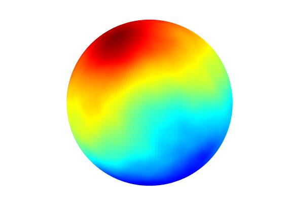
(a) Sample of solution.

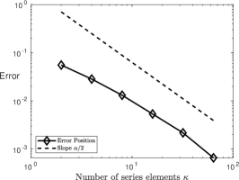
(b) Errors in position.

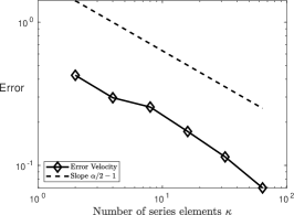
(c) Errors in velocity.

Figure 1. Sample and mean-square errors of the approximation of the stochastic wave equation with angular power spectrum of the $Q$-Wiener process with parameter $\alpha=3$ and $100$ Monte Carlo samples.

In these figures, one observes that the simulation results match the theoretical results from Proposition 4.1. In addition, in order to illustrate the structure of the solution $u$ in dependence of the decay of the angular power spectrum, we include samples next to the convergence plots.

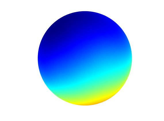
(a) Sample of solution.

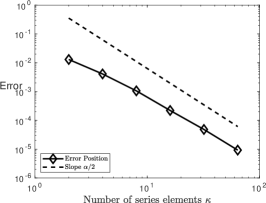
(b) Errors in position.

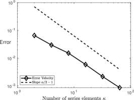
(c) Errors in velocity.

Figure 2. Sample and mean-square errors of the approximation of the stochastic wave equation with angular power spectrum of the $Q$-Wiener process with parameter $\alpha=5$ and $100$ Monte Carlo samples.

In order to illustrate Remark 4.2 on the possibility of taking the parameter $0<\alpha<2$ to show convergence in the first component, we repeat the previous numerical experiments with $\alpha=1$. The results are presented in Figure 3. There, for such non-smooth noise, one can observe convergence in the position but not in the velocity. Similar observations were made for time discretizations of stochastic wave equations on domains (that are not manifolds) in [10, 3], for instance.

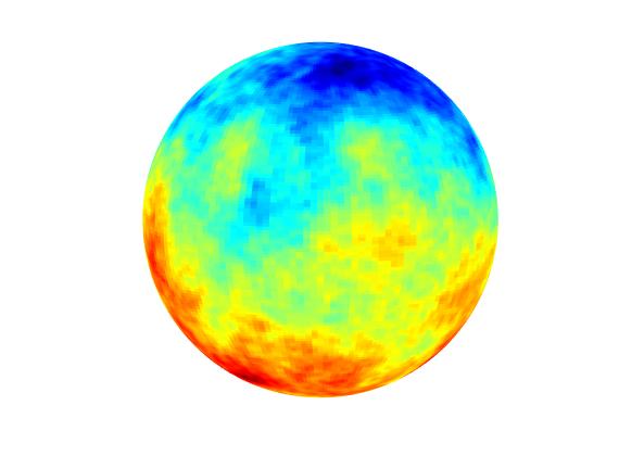
(a) Sample of solution.

(b) Errors in position.

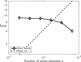
(c) Errors in velocity.

Figure 3. Sample and mean-square errors of the approximation of the stochastic wave equation with angular power spectrum of the $Q$-Wiener process with parameter $\alpha=1$ and $100$ Monte Carlo samples.

In Figure 4 we illustrate the convergence rates with respect to the regularity of the initial position from Proposition 4.1. To ensure that the regularity of the initial position dominates the error, we choose $\alpha=10$ and a random initial position $v_{1}$ scaled such that it belongs to $H^{\beta}(\mathbb{S}^{2})$ with $\beta=2$. The expected convergence rates are indeed observed in this figure.

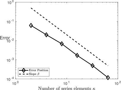
(a) Errors in position.

(b) Errors in velocity.

Figure 4. Mean-square errors of the approximation of the stochastic wave equation with angular power spectrum of the $Q$-Wiener process with parameter $\alpha=10$ and $v_{1}\in H^{\beta}(\mathbb{S}^{2})$ for $\beta=2$ and $100$ Monte Carlo samples.

Errors of one path of the stochastic wave equation to the corresponding error plots from the previous figures (Figure 1 and Figure 2) are presented in Figure 5. The observed convergence rates coincide with the theoretical results on $\mathbb{P}$-almost sure convergence in the second part of Proposition 4.1.

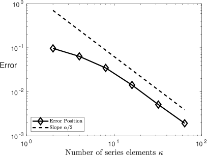
(a) Angular power spectrum with parameter $\alpha=3$.

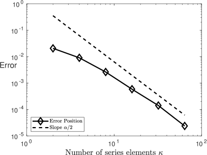
(b) Angular power spectrum with parameter $\alpha=5$.

Figure 5. Error of the approximation of a path of the stochastic wave equation with different angular power spectra of the $Q$-Wiener process.

Let us now illustrate the weak rates of convergence from Proposition 4.3 and Proposition 4.5. We consider a “reference” solution at time $T=1$ with $\kappa=2^{7}$. The initial values are taken to be $v_{1}=v_{2}=0$. The test functions are given by $\varphi(u)=\|u\|_{L^{2}(\mathbb{S}^{2})}^{2}$ and $\varphi(u)=\exp(-\|u\|_{L^{2}(\mathbb{S}^{2})}^{2})$. Observe that the second test function is of class $C^{2}$, bounded and with bounded derivatives. Proposition 4.3 and Proposition 4.5 guarantee that the weak rates will be essentially twice the strong rates in both cases. This is confirmed for $\alpha=3$ in Figure 6.

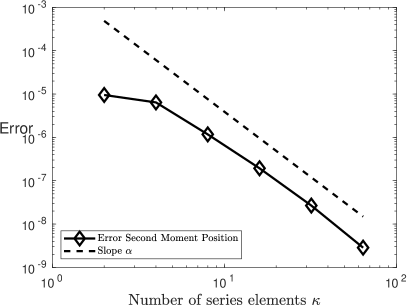
(a) $\varphi(u)=\|u\|_{L^{2}(\mathbb{S}^{2})}^{2}$.

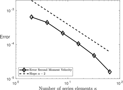
(b) $\varphi(u)=\|u\|_{L^{2}(\mathbb{S}^{2})}^{2}$.

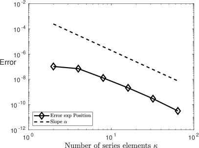
(c) $\varphi(u)=\exp(-\|u\|_{L^{2}(\mathbb{S}^{2})}^{2})$.

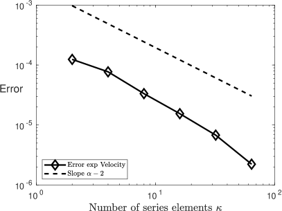
(d) $\varphi(u)=\exp(-\|u\|_{L^{2}(\mathbb{S}^{2})}^{2})$.

Figure 6. Weak errors of the approximation of the stochastic wave equation with angular power spectrum of the $Q$-Wiener process with parameter $\alpha=3$ and $1000$ Monte Carlo samples. Left column shows position, right column velocity.

6. Further extensions

In this section, we extend some of the above results first to the case of the stochastic wave equation on higher-dimensional spheres $\mathbb{S}^{d-1}$, for some integer $d>3$, and second to the case of a free stochastic Schrödinger equation on the sphere $\mathbb{S}^{2}$. We keep this section concise and focus on strong and $\mathbb{P}$-a.s. convergence.

6.1. The stochastic wave equation on $\mathbb{S}^{d-1}$

Let us consider the more general situation of the stochastic wave equation on the unit sphere $\mathbb{S}^{d-1}=\{x\in\mathbb{R}^{d},\|x\|_{\mathbb{R}^{d}}=1\}$ embedded into $\mathbb{R}^{d}$. The angular distance of two points $x$ and $y$ on $\mathbb{S}^{d-1}$ is given in the same way as on $\mathbb{S}^{2}$, see Section 2. Let us denote by $(S_{\ell,m},\ell\in\mathbb{N}_{0},m=1,\ldots,h(\ell,d))$ the spherical harmonics on $\mathbb{S}^{d-1}$, where

$$h(\ell,d)=(2\ell+d-2)\frac{(\ell+d-3)!}{(d-2)!\,\ell!}.$$

Using the same setup as in [29] which goes back to [35], a centered isotropic Gaussian random field $Z$ on $\mathbb{S}^{d-1}$ admits a Karhunen–Loève expansion

$$Z(x)=\sum_{\ell=0}^{\infty}\sum_{m=1}^{h(\ell,d)}a_{\ell,m}S_{\ell,m}(x),$$

where $(a_{\ell,m},\ell\in\mathbb{N}_{0},m=1,\ldots,h(\ell,d))$ is a sequence of independent Gaussian random variables satisfying

$$\operatorname{\mathbb{E}}[a_{\ell,m}]=0,\quad\operatorname{\mathbb{E}}[a_{\ell,m}a_{\ell^{\prime},m^{\prime}}]=A_{\ell}\delta_{\ell\ell^{\prime}}\delta_{mm^{\prime}}$$

for $\ell,\ell^{\prime}\in\mathbb{N}_{0}$ and $m=1,\ldots,h(\ell,d)$, $m^{\prime}=1,\ldots,h(\ell^{\prime},d)$ and

$$\sum_{\ell=0}^{\infty}A_{\ell}\,h(\ell,d)<+\infty.$$

The series converges with probability one and in $L^{p}(\Omega;\mathbb{R})$ as well as in $L^{2}(\Omega;L^{p}(\mathbb{S}^{d-1}))$, $p\geq 1$. Denoting by $(A_{\ell},\ell\in\mathbb{N}_{0})$ the angular power spectrum of $Z$ for $\mathbb{S}^{d-1}$ in analogy to what was done for $\mathbb{S}^{2}$, we can rewrite

$$Z=\sum_{\ell=0}^{\infty}\sum_{m=1}^{h(\ell,d)}a_{\ell,m}S_{\ell,m}=\sum_{\ell=0}^{\infty}\sqrt{A_{\ell}}\sum_{m=1}^{h(\ell,d)}X_{\ell,m}S_{\ell,m},$$

where $(X_{\ell,m},\ell\in\mathbb{N}_{0},m=1,\ldots,h(\ell,d))$ is the sequence of independent, standard normally distributed random variables derived by $X_{\ell,m}=a_{\ell,m}/\sqrt{A_{\ell}}$. We set

$$Z^{\kappa}=\sum_{\ell=0}^{\kappa}\sqrt{A_{\ell}}\sum_{m=1}^{h(\ell,d)}X_{\ell,m}S_{\ell,m}$$

for the corresponding sequence of truncated random fields $(Z^{\kappa},\kappa\in\mathbb{N})$. It is shown in Theorem 5.5 in [29] that these approximations converge to the random field $Z$ in $L^{p}(\Omega;L^{2}(\mathbb{S}^{d-1}))$ and $\mathbb{P}$-almost surely with error bounds

(10) $$\|Z-Z^{\kappa}\|_{L^{p}(\Omega;L^{2}(\mathbb{S}^{d-1}))}\leq C_{p}\cdot\kappa^{-(\alpha+1-d)/2}$$

for $\kappa>\ell_{0}$ and for all $\delta<(\alpha+1-d)/2$

(11) $$\|Z-Z^{\kappa}\|_{L^{2}(\mathbb{S}^{d-1})}\leq\kappa^{-\delta},\quad\mathbb{P}\text{-a.s.},$$

where $A_{\ell}\leq C\cdot\ell^{-\alpha}$ for $\ell\geq\ell_{0}$. This generalizes Theorem 2.2 above and leads to convergence rates that depend also on the dimension of the sphere.

Similarly to (1) in Section 2, we introduce a $Q$-Wiener process $(W(t),t\in\mathbb{T})$ on some finite interval $\mathbb{T}=[0,T]$ with values in $L^{2}(\mathbb{S}^{d-1})$ by the expansion

(12) $$W(t,y)=\sum_{\ell=0}^{\infty}\sum_{m=1}^{h(\ell,d)}a^{\ell,m}(t)S_{\ell,m}(y)=\sum_{\ell=0}^{\infty}\sqrt{A_{\ell}}\sum_{m=1}^{h(\ell,d)}\beta^{\ell,m}(t)S_{\ell,m}(y),$$

where $(\beta^{\ell,m},\ell\in\mathbb{N}_{0},m=1,\ldots,h(\ell,d))$ is a sequence of independent, real-valued Brownian motions.

We next recall that the Laplace–Beltrami operator $\Delta_{\mathbb{S}^{d-1}}$ on $\mathbb{S}^{d-1}$ has the spherical harmonics $(S_{\ell,m},\ell\in\mathbb{N}_{0},m=1,\ldots,h(\ell,d))$ as eigenbasis with eigenvalues given by

$$\Delta_{\mathbb{S}^{d-1}}S_{\ell,m}=-\ell(\ell+d-2)S_{\ell,m}$$

for $\ell\in\mathbb{N}_{0}$ and $m=1,\ldots,h(\ell,d)$ (see, e. g., [4, Sec. 3.3]).

We introduce Sobolev spaces on $\mathbb{S}^{d-1}$, similarly to $\mathbb{S}^{2}$, which are given for a smoothness index $s\in\mathbb{R}$ by

$$H^{s}(\mathbb{S}^{d-1})=(\text{Id}-\Delta_{\mathbb{S}^{d-1}})^{-s/2}L^{2}(\mathbb{S}^{d-1})$$

together with the norm

$$\|f\|_{H^{s}(\mathbb{S}^{d-1})}=\|(\text{Id}-\Delta_{\mathbb{S}^{d-1}})^{s/2}f\|_{L^{2}(\mathbb{S}^{d-1})}$$

for some $f\in H^{s}(\mathbb{S}^{d-1})$. We also denote $H^{0}(\mathbb{S}^{d-1})=L^{2}(\mathbb{S}^{d-1})$.

The stochastic wave equation on $\mathbb{S}^{d-1}$ is defined as

(13) $$\partial_{tt}u(t)-\Delta_{\mathbb{S}^{d-1}}u(t)=\dot{W}(t),$$

with initial conditions $u(0)=v_{1}\in L^{2}(\Omega;L^{2}(\mathbb{S}^{d-1}))$ and $\partial_{t}u(0)=v_{2}\in L^{2}(\Omega;L^{2}(\mathbb{S}^{d-1}))$, where $t\in\mathbb{T}=[0,T]$, $T<+\infty$. The notation $\dot{W}$ stands for the formal derivative of the $Q$-Wiener process.

Denoting as before the velocity of the solution by $u_{2}=\partial_{t}u_{1}=\partial_{t}u$, one can rewrite (13) as

$$\mathop{}\!\mathrm{d}X(t) =AX(t)\,\mathop{}\!\mathrm{d}t+G\,\mathop{}\!\mathrm{d}W(t)$$

(14) $$X(0) =X_{0},$$

where

$$A=\begin{pmatrix}0&I\\ \Delta_{\mathbb{S}^{d-1}}&0\end{pmatrix},\quad G=\begin{pmatrix}0\\ I\end{pmatrix},\quad X=\begin{pmatrix}u_{1}\\ u_{2}\end{pmatrix},\quad X_{0}=\begin{pmatrix}v_{1}\\ v_{2}\end{pmatrix}.$$

Existence of a unique mild solution follows as before.

Using the same ansatz as in Section 3 with respect to the spherical harmonics on $\mathbb{S}^{d-1}$

(15) $$u_{1}(t)=\displaystyle\sum_{\ell=0}^{\infty}\sum_{m=1}^{h(\ell,d)}u_{1}^{\ell,m}(t)S_{\ell,m}\quad\text{and}\quad u_{2}(t)=\displaystyle\sum_{\ell=0}^{\infty}\sum_{m=1}^{h(\ell,d)}u_{2}^{\ell,m}(t)S_{\ell,m}$$

we obtain

$$u_{1}^{\ell,m}(t) =v_{1}^{\ell,m}+\int_{0}^{t}u_{2}^{\ell,m}(s)\,\mathop{}\!\mathrm{d}s$$

$$u_{2}^{\ell,m}(t) =v_{2}^{\ell,m}-\ell(\ell+d-2)\int_{0}^{t}u_{1}^{\ell,m}(s)\,\mathop{}\!\mathrm{d}s+a^{\ell,m}(t),$$

where $v_{1}^{\ell,m}$, $v_{2}^{\ell,m}$, resp. $a^{\ell,m}$ are the coefficients of the expansions of the initial values $v_{1}$ and $v_{2}$, resp. weighted Brownian motion in the expansion of the noise (12).

Similarly to (6), the variation of constants formula yields

$$\begin{cases}u_{1}^{\ell,m}(t)&\displaystyle=R^{\ell}_{2}(t)v_{1}^{\ell,m}+R^{\ell}_{1}(t)v_{2}^{\ell,m}+\hat{W}_{1}^{\ell,m}(t)\\ u_{2}^{\ell,m}(t)&\displaystyle=-(\ell(\ell+d-2))R^{\ell}_{1}(t)v_{1}^{\ell,m}+R^{\ell}_{2}(t)v_{2}^{\ell,m}+\hat{W}_{2}^{\ell,m}(t),\end{cases}$$

where

$$\hat{W}^{\ell,m}(t)=\begin{pmatrix}\hat{W}_{1}^{\ell,m}(t)\\ \hat{W}_{2}^{\ell,m}(t)\end{pmatrix}=\displaystyle\int_{0}^{t}R^{\ell}(t-s)\,\mathop{}\!\mathrm{d}a^{\ell,m}(s)$$

with

$$R^{\ell}(t)=\begin{pmatrix}R^{\ell}_{1}(t)\\ R^{\ell}_{2}(t)\end{pmatrix}=\begin{pmatrix}(\ell(\ell+d-2))^{-1/2}\sin(t(\ell(\ell+d-2))^{1/2})\\ \cos(t(\ell(\ell+d-2))^{1/2})\end{pmatrix}$$

for $\ell\neq 0$ and

$$\hat{W}^{0,0}(t)=\begin{pmatrix}\hat{W}_{1}^{0,0}(t)\\ \hat{W}_{2}^{0,0}(t)\end{pmatrix}=\begin{pmatrix}\displaystyle\int_{0}^{t}a^{0,0}(s)\,\mathop{}\!\mathrm{d}s\\ a^{0,0}(t)\end{pmatrix}.$$

Note that the only change compared to Section 3 is the value of the coefficients given by the eigenvalues $\Delta_{\mathbb{S}^{d-1}}$ and the renaming of the spherical harmonics.

As in Section 4, we approximate the solution to the stochastic wave equation (6.1) by truncation of the series expansion at some finite index $\kappa>0$ and obtain

(16) $$u_{1}^{\kappa}(t_{j})=\displaystyle\sum_{\ell=0}^{\kappa}\sum_{m=1}^{h(\ell,d)}u_{1}^{\ell,m}(t_{j})S_{\ell,m}\quad\text{and}\quad u_{2}^{\kappa}(t_{j})=\displaystyle\sum_{\ell=0}^{\kappa}\sum_{m=1}^{h(\ell,d)}u_{2}^{\ell,m}(t_{j})S_{\ell,m}.$$

Then replacing the eigenvalues $-\ell(\ell+1)$ with $-\ell(\ell+d-2)$, the multiplicity of the eigenvalues $2\ell+1$ with $h(\ell,d)$ and applying (10) and (11) instead of Theorem 2.2 in the proof of Proposition 4.1 yields directly the following extension of Proposition 4.1.

Proposition 6.1.

Let $t\in\mathbb{T}$ and $0=t_{0}<\cdots<t_{n}=t$ be a discrete time partition for $n\in\mathbb{N}$, which yields a recursive representation of the solution $X=(u_{1},u_{2})$ of the stochastic wave equation (6.1) on $\mathbb{S}^{d-1}$ given by (15). Assume that the initial values satisfy $v_{1}\in H^{\beta}(\mathbb{S}^{d-1})$ and $v_{2}\in H^{\gamma}(\mathbb{S}^{d-1})$. Furthermore, assume that there exist $\ell_{0}\in\mathbb{N}$, $\alpha>2$, and a constant $C>0$ such that the angular power spectrum of the driving noise $(A_{\ell},\ell\in\mathbb{N}_{0})$ satisfies $A_{\ell}\leq C\cdot\ell^{-\alpha}$ for all $\ell>\ell_{0}$. Then, the error of the approximate solution $X^{\kappa}=(u_{1}^{\kappa},u_{2}^{\kappa})$, given by (16), is bounded uniformly on any finite time interval and independently of the time discretization by

$$\|u_{1}(t)-u_{1}^{\kappa}(t)\|_{L^{p}(\Omega;L^{2}(\mathbb{S}^{d-1}))} \leq\hat{C}_{p}\cdot\left(\kappa^{-(\alpha+3-d)/2}+\kappa^{-\beta}\|v_{1}\|_{H^{\beta}(\mathbb{S}^{d-1})}+\kappa^{-(\gamma+1)}\|v_{2}\|_{H^{\gamma}(\mathbb{S}^{d-1})}\right)$$

$$\|u_{2}(t)-u_{2}^{\kappa}(t)\|_{L^{p}(\Omega;L^{2}(\mathbb{S}^{d-1}))} \leq\hat{C}_{p}\cdot\left(\kappa^{-(\alpha+1-d)/2}+\kappa^{-(\beta-1)}\|v_{1}\|_{H^{\beta}(\mathbb{S}^{d-1})}+\kappa^{-\gamma}\|v_{2}\|_{H^{\gamma}(\mathbb{S}^{d-1})}\right)$$

for all $p\geq 1$ and $\kappa>\ell_{0}$, where $\hat{C}_{p}$ is a constant that may depend on $p$, $C$, $T$, and $\alpha$.

Additionally, the error is bounded uniformly in time, independently of the time discretization, and asymptotically in $\kappa$ by

$$\|u_{1}(t)-u_{1}^{\kappa}(t)\|_{L^{2}(\mathbb{S}^{d-1})} \leq\kappa^{-\delta},\quad\mathbb{P}\text{-a.s.}$$

$$\|u_{2}(t)-u_{2}^{\kappa}(t)\|_{L^{2}(\mathbb{S}^{d-1})} \leq\kappa^{-(\delta-1)},\quad\mathbb{P}\text{-a.s.}$$

for all $\delta<\min((\alpha+3-d)/2,\beta,\gamma+1)$.

6.2. The free stochastic Schrödinger equation on $\mathbb{S}^{2}$

We consider efficient simulations of paths of solutions to the free stochastic Schrödinger equation on the sphere $\mathbb{S}^{2}$

(17) $$\mathrm{i}\partial_{t}u(t)=\Delta_{\mathbb{S}^{2}}u(t)+\dot{W}(t),$$

with initial condition (possibly complex-valued) $u(0)\in L^{2}(\Omega;L^{2}(\mathbb{S}^{2}))$. Here, the unknown $u(t)=u_{R}(t)+\mathrm{i}u_{I}(t)$, with $t\in[0,T]$ for some $T<+\infty$, is a complex valued stochastic process. Furthermore, the notation $\dot{W}$ stands for the formal derivative of the (real-valued) $Q$-Wiener process with series expansion (1).

Considering the real and imaginary parts of the above SPDE, one can rewrite (17) as

(18) $$\begin{split}\mathop{}\!\mathrm{d}X(t)&=AX(t)\,\mathop{}\!\mathrm{d}t+G\,\mathop{}\!\mathrm{d}W(t)\\ X(0)&=X_{0},\end{split}$$

where

$$A=\begin{pmatrix}0&\Delta_{\mathbb{S}^{2}}\\ -\Delta_{\mathbb{S}^{2}}&0\end{pmatrix},\quad G=\begin{pmatrix}0\\ -I\end{pmatrix},\quad X=\begin{pmatrix}u_{R}\\ u_{I}\end{pmatrix},\quad X_{0}=\begin{pmatrix}u_{R}(0)\\ u_{I}(0)\end{pmatrix}.$$

The existence of a mild form of the abstract formulation (18) of the stochastic Schrödinger equation on the sphere follows like for the above stochastic wave equation. The mild form reads

(19) $$X(t)=\mathrm{e}^{tA}X_{0}+\int_{0}^{t}\mathrm{e}^{(t-s)A}G\,\mathop{}\!\mathrm{d}W(s)$$

with the semigroup

$$\mathrm{e}^{tA}=\begin{pmatrix}\cos(t\Delta_{\mathbb{S}^{2}})&\sin(t\Delta_{\mathbb{S}^{2}})\\ -\sin(t\Delta_{\mathbb{S}^{2}})&\cos(t\Delta_{\mathbb{S}^{2}})\end{pmatrix}.$$

Finally, one obtains the integral formulation of the above problem as

$$\begin{cases}u_{R}(t)&\displaystyle=u_{R}(0)+\int_{0}^{t}\Delta_{\mathbb{S}^{2}}u_{I}(s)\,\mathop{}\!\mathrm{d}s\\ u_{I}(t)&\displaystyle=u_{I}(0)-\int_{0}^{t}\Delta_{\mathbb{S}^{2}}u_{R}(s)\,\mathop{}\!\mathrm{d}s-W(t).\end{cases}$$

As it was done for the stochastic wave equation in Section 3, one can make the following ansatz for the real and imaginary part of solutions to (19)

$$u_{R}(t)=\sum_{\ell=0}^{\infty}\sum_{m=-\ell}^{\ell}u_{R}^{\ell,m}Y_{\ell,m}\quad\text{and}\quad u_{I}(t)=\sum_{\ell=0}^{\infty}\sum_{m=-\ell}^{\ell}u_{I}^{\ell,m}Y_{\ell,m}$$

and find the following system of equations defining the coefficients of these expansions:

$$\begin{cases}u_{R}^{\ell,m}(t)&\displaystyle=\cos(t(\ell(\ell+1))^{1/2})v_{R}^{\ell,m}+\sin(t(\ell(\ell+1))^{1/2})v_{I}^{\ell,m}+\hat{W}_{R}^{\ell,m}(t)\\ u_{I}^{\ell,m}(t)&\displaystyle=-\sin(t(\ell(\ell+1))^{1/2})v_{R}^{\ell,m}+\cos(t(\ell(\ell+1))^{1/2})v_{I}^{\ell,m}+\hat{W}_{I}^{\ell,m}(t),\end{cases}$$

where

$$\hat{W}^{\ell,m}(t)=\begin{pmatrix}\hat{W}_{R}^{\ell,m}(t)\\ \hat{W}_{I}^{\ell,m}(t)\end{pmatrix}=\begin{pmatrix}\displaystyle\int_{0}^{t}\sin((t-s)(\ell(\ell+1))^{1/2})\,\mathop{}\!\mathrm{d}a^{\ell,m}(s)\\ \displaystyle\int_{0}^{t}\cos((t-s)(\ell(\ell+1))^{1/2})\,\mathop{}\!\mathrm{d}a^{\ell,m}(s)\end{pmatrix}$$

and $v_{R}^{\ell,m}$, resp. $v_{I}^{\ell,m}$, are the coefficients of the real, resp. imaginary, part of the initial value $u(0)$.

It is clear that the analysis from Section 4 can directly be extend to the case of the stochastic Schrödinger equation on the sphere (17). The errors in the truncation procedure, denoted by $u_{R}^{\kappa}$ and $u_{I}^{\kappa}$, of the above ansatz are given by the following proposition (presented for zero initial data for simplicity).

Proposition 6.2.

Let $t\in\mathbb{T}=[0,T]$ and $0=t_{0}<\ldots<t_{n}=t$ be a discrete time partition for $n\in\mathbb{N}$, which yields a recursive representation of the solution $X=(u_{R},u_{I})$ of the stochastic Schrödinger equation on the sphere (18) with initial data $u(0)=0$. Assume that there exist $\ell_{0}\in\mathbb{N}$, $\alpha>2$, and a constant $C>0$ such that the angular power spectrum of the driving noise $(A_{\ell},\ell\in\mathbb{N}_{0})$ decays with $A_{\ell}\leq C\cdot\ell^{-\alpha}$ for all $\ell>\ell_{0}$. Then, the error of the approximate solution $X^{\kappa}=(u_{R}^{\kappa},u_{I}^{\kappa})$ is bounded uniformly in time and independently of the time discretization by

$$\|u_{R}(t)-u_{R}^{\kappa}(t)\|_{L^{p}(\Omega;L^{2}(\mathbb{S}^{2}))} \leq\hat{C}_{p}\cdot\kappa^{-(\alpha/2-1)}$$

$$\|u_{I}(t)-u_{I}^{\kappa}(t)\|_{L^{p}(\Omega;L^{2}(\mathbb{S}^{2}))} \leq\hat{C}_{p}\cdot\kappa^{-(\alpha/2-1)}$$

for all $p\geq 1$ and $\kappa>\ell_{0}$, where $\hat{C}_{p}$ is a constant that may depend on $p$, $C$, $T$, and $\alpha$.

On top of that, the error is bounded uniformly in time, independently of the time discretization, and asymptotically in $\kappa$ by

$$\|u_{R}(t)-u_{R}^{\kappa}(t)\|_{L^{2}(\mathbb{S}^{2})} \leq\kappa^{-(\delta-1)},\quad\mathbb{P}\text{-a.s.}$$

$$\|u_{I}(t)-u_{I}^{\kappa}(t)\|_{L^{2}(\mathbb{S}^{2})} \leq\kappa^{-(\delta-1)},\quad\mathbb{P}\text{-a.s.}$$

for all $\delta<\alpha/2$.

Since the proof of this proposition follows the lines of the proof of Proposition 4.1, we omit it and instead present some numerical experiments illustrating these theoretical results.

We compute the errors when approximating solutions to (17) for various truncation indices $\kappa$ for a $Q$-Wiener process with parameter $\alpha=4$. All other parameters are the same as in Section 5. In Figure 7, we display a sample at time $T=1$ and a strong convergence plot of the real part of the numerical approximation, as well as errors in the approximation of a path (imaginary part) to the stochastic Schrödinger equation on the sphere. These illustrations are in agreement with the results from Proposition 6.2.

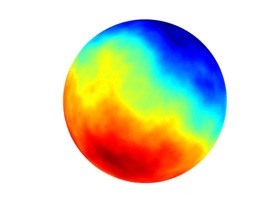
(a) Sample of solution.

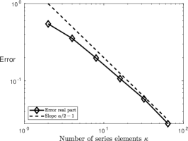
(b) Strong errors (real part).

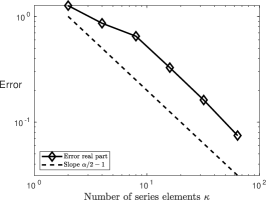
(c) Error in approximation of one path (imaginary part).

Figure 7. Sample, mean-square errors, and error of one path of the approximation of the stochastic Schrödinger equation with angular power spectrum of the $Q$-Wiener process with parameter $\alpha=4$ and $100$ Monte Carlo samples (for the mean-square errors).

References

• [1] Adam Andersson, Raphael Kruse, and Stig Larsson. Duality in refined Sobolev–Malliavin spaces and weak approximations of SPDE. Stoch. PDE: Anal. Comp., 4(1):113–149, 2016.
• [2] Vo V. Anh, Philip Broadbridge, Andriy Olenko, and Yu Guang Wang. On approximation for fractional stochastic partial differential equations on the sphere. Stoch. Environ. Res. Risk Assess, 32(9):2585–2603, 2018.
• [3] Rikard Anton, David Cohen, Stig Larsson, and Xiaojie Wang. Full discretization of semilinear stochastic wave equations driven by multiplicative noise. SIAM J. Numer. Anal., 54(2):1093–1119, 2016.
• [4] Kendall Atkinson and Weimin Han. Spherical Harmonics and Approximations on the Unit Sphere: An Introduction, volume 2044 of Lecture Notes in Mathematics. Springer-Verlag, 2012.
• [5] Charles-Edouard Bréhier, Martin Hairer, and Andrew M. Stuart. Weak error estimates for trajectories of SPDEs under spectral Galerkin discretization. J. Comp. Math., 36(2):159–182, 2018.
• [6] Phil Broadbridge, Alexander D. Kolesnik, Nikolai Leonenko, and Andriy Olenko. Random spherical hyperbolic diffusion. J. Stat. Phys., 177(5):889–916, 2019.
• [7] Julia Charrier. Strong and weak error estimates for elliptic partial differential equations with random coefficients. SIAM J. Numer. Anal., 50(1):216–246, 2012.
• [8] Jorge Clarke De la Cerda, Alfredo Alegría, and Emilio Porcu. Regularity properties and simulations of Gaussian random fields on the sphere cross time. Electron. J. Stat., 12(1):399–426, 2018.
• [9] Richard H. Clayton. Dispersion of recovery and vulnerability to re-entry in a model of human atrial tissue with simulated diffuse and focal patterns of fibrosis. Frontiers in Physiology, 9:1052, 2018.
• [10] David Cohen, Stig Larsson, and Magdalena Sigg. A trigonometric method for the linear stochastic wave equation. SIAM J. Numer. Anal., 51(1):204–222, 2013.
• [11] Giuseppe Da Prato and Jerzy Zabczyk. Stochastic Equations in Infinite Dimensions, volume 152 of Encyclopedia of Mathematics and its Applications. Cambridge University Press, second edition, 2014.
• [12] Robert Dalang, Davar Khoshnevisan, Carl Mueller, David Nualart, and Yimin Xiao. A Minicourse on Stochastic Partial Differential Equations, volume 1962 of Lecture Notes in Mathematics. Springer-Verlag, 2009. Held at the University of Utah, Salt Lake City, UT, May 8–19, 2006, Edited by Khoshnevisan and Firas Rassoul-Agha.
• [13] Arnaud Debussche and Jacques Printems. Weak order for the discretization of the stochastic heat equation. Math. Comput., 78(266):845–863, 2009.
• [14] Xavier Fernique. Intégrabilité des vecteurs gaussiens. C. R. Acad. Sci., Paris, Sér. A, 270:1698–1699, 1970.
• [15] Joshua H. Goldwyn and Eric Shea-Brown. The what and where of adding channel noise to the Hodgkin–Huxley equations. PLOS Comp. Biol., 7(11):1–9, 11 2011.
• [16] Philipp Harms and Marvin S. Müller. Weak convergence rates for stochastic evolution equations and applications to nonlinear stochastic wave, HJMM, stochastic Schrödinger and linearized stochastic Korteweg–de Vries equations. Z. Angew. Math. Phys., 70(1):Paper No. 16, 28, 2019.
• [17] Klaus Hasselmann. Stochastic climate models part I. Theory. Tellus, 28(6):473–485, 1976.
• [18] Lukas Herrmann, Kristin Kirchner, and Christoph Schwab. Multilevel approximation of Gaussian random fields: fast simulation. Math. Models Methods Appl. Sci., 30(1):181–223, 2020.
• [19] Lukas Herrmann, Annika Lang, and Christoph Schwab. Numerical analysis of lognormal diffusions on the sphere. Stoch. PDE: Anal. Comp., 6(1):1–44, 2018.
• [20] Ladislas Jacobe de Naurois, Arnulf Jentzen, and Timo Welti. Lower bounds for weak approximation errors for spatial spectral galerkin approximations of stochastic wave equations. In Andreas Eberle, Martin Grothaus, Walter Hoh, Moritz Kassmann, Wilhelm Stannat, and Gerald Trutnau, editors, Stochastic Partial Differential Equations and Related Fields, pages 237–248, Cham, 2018. Springer International Publishing.
• [21] Mehran Kardar, Giorgio Parisi, and Yi-Cheng Zhang. Dynamic scaling of growing interfaces. Phys. Rev. Lett., 56:889–892, 1986.
• [22] Yoshihito Kazashi and Quoc T. Le Gia. A non-uniform discretization of stochastic heat equations with multiplicative noise on the unit sphere. J. Complexity, 50:43–65, 2019.
• [23] Mihály Kovács, Annika Lang, and Andreas Petersson. Weak convergence of fully discrete finite element approximations of semilinear hyperbolic SPDEs with additive noise. ESAIM:M2AN, 54(6):2199–2227, 2020.
• [24] Mihály Kovács, Stig Larsson, and Fredrik Lindgren. Weak convergence of finite element approximations of linear stochastic evolution equations with additive noise. BIT Num. Math, 52(1):85–108, 2012.
• [25] Yuriy V. Kozachenko and L. F. Kozachenko. Modeling Gaussian isotropic random fields on a sphere. J. Math. Sci., 107(2):3751–3757, 2001.
• [26] Xiaohong Lan and Domenico Marinucci. On the dependence structure of wavelet coefficients for spherical random fields. Stochastic Process. Appl., 119(10):3749–3766, 2009.
• [27] Xiaohong Lan, Domenico Marinucci, and Yimin Xiao. Strong local nondeterminism and exact modulus of continuity for spherical Gaussian fields. Stochastic Process. Appl., 128(4):1294–1315, 2018.
• [28] Annika Lang, Stig Larsson, and Christoph Schwab. Covariance structure of parabolic stochastic partial differential equations. Stoch. PDE: Anal. Comp., 1(2):351–364, 2013.
• [29] Annika Lang and Christoph Schwab. Isotropic Gaussian random fields on the sphere: regularity, fast simulation and stochastic partial differential equations. Ann. Appl. Probab., 25(6):3047–3094, 2015.
• [30] Quoc Thong Le Gia, Ian H. Sloan, Robert S. Womersley, and Yu Guang Wang. Isotropic sparse regularization for spherical harmonic representations of random fields on the sphere. Appl. Comput. Harmon. Anal., 49(1):257–278, 2020.
• [31] Domenico Marinucci and Giovanni Peccati. Random Fields on the Sphere. Representation, Limit Theorems and Cosmological Applications. Cambridge University Press, 2011.
• [32] Mitsuo Morimoto. Analytic Functionals on the Sphere, volume 178 of Translations of Mathematical Monographs. American Mathematical Society, 1998.
• [33] Gábor Szegő. Orthogonal Polynomials, volume XXIII of Colloquium Publications. American Mathematical Society, fourth edition, 1975.
• [34] Xiaojie Wang. An exponential integrator scheme for time discretization of nonlinear stochastic wave equation. J. Sci. Comput., 64(1):234–263, 2015.
• [35] Myhailo I. Yadrenko. Spectral Theory of Random Fields. Translation Series in Mathematics and Engineering. Optimization Software, Inc., Publications Division; Springer-Verlag, 1983. Transl. from the Russian.