Novel Deep neural networks for solving
Bayesian statistical inverse problems

Abstract

We consider the simulation of Bayesian statistical inverse problems governed by large-scale linear and nonlinear partial differential equations (PDEs). Markov chain Monte Carlo (MCMC) algorithms are standard techniques to solve such problems. However, MCMC techniques are computationally challenging as they require several thousands of forward PDE solves. The goal of this paper is to introduce a fractional deep neural network based approach for the forward solves within an MCMC routine. Moreover, we discuss some approximation error estimates and illustrate the efficiency of our approach via several numerical examples.

1 Introduction

Large-scale statistical inverse problems governed by partial differential equations (PDEs) are increasingly found in different areas of computational science and engineering [5, 9, 10, 20, 36]. The basic use of this class of problems is to recover certain physical quantities from limited and noisy observations. They are generally computationally demanding and can be solved using the Bayesian framework [9, 18, 20]. In the Bayesian approach to statistical inverse problems, one models the solution as a posterior distribution of the unknown parameters conditioned on the observations. Such mathematical formulations are often ill-posed and regularization is introduced in the model via prior information. The posterior distribution completely characterizes the uncertainty in the model. Once it has been computed, statistical quantities of interest can then be obtained from the posterior distribution. Unfortunately, many problems of practical relevance do not admit analytic representation of the posterior distribution. Thus, the posterior distributions are generally sampled using Markov chain Monte Carlo (MCMC)-type schemes.

We point out here that a large number of samples are generally needed by MCMC methods to obtain convergence. This makes MCMC methods computationally intensive to simulate Bayesian inverse problems. Moreover, for statistical inverse problems governed by PDEs, one needs to solve the forward problem corresponding to each MCMC sample. This task further increases the computational complexity of the problem, especially if the governing PDE is a large-scale nonlinear PDE [18]. Hence, it is reasonable to construct a computationally cheap surrogate to replace the forward model solver [40]. Problems that involve large numbers of input parameters often lead to the so-called curse of dimensionality. Projection-based reduced-order models e.g., reduced basis methods and the discrete empirical interpolation method (DEIM) are typical examples of dimensionality reduction methods for tackling parametrized PDEs [1, 6, 12, 17, 21, 33, 44]. However, they are intrusive by design in the sense that they do not allow reuse of existing codes in the forward solves, especially for nonlinear forward models. To mitigate this computational issue, the goal of this work is to demonstrate the use of deep neural networks (DNN) to construct surrogate models specifically for nonlinear parametrized PDEs governing statistical Bayesian inverse problems. In particular, we will focus on fractional Deep Neural Networks (fDNN) which have been recently introduced and applied to classification problems [2].

The use of DNNs for surrogate modeling in the framework of PDEs has received increasing attention in recent years, see e.g., [13, 25, 29, 41, 43, 45, 49, 52, 54] and the references therein. Some of these references also cover the type of Bayesian inverse problems considered in our paper. To accelerate or replace computationally-expensive PDE solves, a DNN is trained to approximate the mapping from parameters in the PDE to observations obtained from its solution. In a supervised learning setting, training data consisting of inputs and outputs are available and the learning problem aims at tuning the weights of the DNN. To obtain an effective surrogate model, it is desirable to train the DNN to a high accuracy.

We consider a different approach than the aforementioned works. We propose novel dynamical systems based neural networks which allow connectivity among all the network layers. Specifically, we consider a fractional DNN technique recently proposed in [2] in the framework of classification problems. We note that [2] is motivated by [26]. Both papers are in the spirit of the push to develop rigorous mathematical models for the analysis and understanding of DNNs. The idea is to consider DNNs as dynamical systems. More precisely, in [7, 26, 28], DNN is thought of as an optimization problem constrained by a discrete ordinary differential equation (ODE). As pointed out in [2], designing the DNN solution algorithms at the continuous level has the appealing advantage of architecture independence; in other words, the number of optimization iterations remains the same even if the number of layers is increased. Moreover, [2] specifically considers continuous fractional ODE constraint. Unlike standard DNNs, the resulting fractional DNN allows the network to access historic information of input and gradients across all subsequent layers since all the layers are connected to one another.

We demonstrate that our fractional DNN leads to a significant reduction in the overall computational time used by MCMC algorithms to solve inverse problems, while maintaining accurate evaluation of the relevant statistical quantities. We note here that, although the papers [41, 49, 54] consider DNNs for inverse problems governed by PDEs, the DNNs used in these studies do not, in general, have the optimization-based formulation considered here.

The remainder of the paper is organized as follows: In section 2 we state the generic parametrized PDEs under consideration, as well as discuss the well-known surrogate modeling approaches. Our main DNN algorithm to approximate parametrized PDEs is provided in section 3. We first discuss a ResNet architecture to approximate parametrized PDEs, which is followed by our fractional ResNet (or fractional DNN) approach to carry out the same task. A brief discussion on error estimates has been provided. Next, we discuss the application of fractional DNN to statistical Bayesian inverse problems in section 4. We conclude the paper with several illustrative numerical examples in section 5.

2 Parametrized PDEs

In this section, we present an abstract formulation of the forward problem as a discrete partial differential equation (PDE) depending on parameters. We are interested in the following model which represents (finite element, finite difference or finite volume) discretization of a (possibly nonlinear) parametrized PDE

$$F({\bf{u}}({\boldsymbol{\xi}});{\boldsymbol{\xi}})=0,$$ (1)

where ${\bf{u}}({\boldsymbol{\xi}})\in\mathcal{U}\subset\mathbb{R}^{N_{x}}$ and ${\boldsymbol{\xi}}\in\mathcal{P}\subset\mathbb{R}^{N_{{\boldsymbol{\xi}}}}$ denote the solution of the PDE and the parameter in the model, respectively. Here, $\mathcal{P}$ denotes the parameter domain and $\mathcal{U}$ the solution manifold. For a fixed parameter ${\boldsymbol{\xi}}\in\mathcal{P}$, we seek the solution ${\bf{u}}({\boldsymbol{\xi}})\in\mathcal{U}$. In other words, we have the functional relation given by the parameter-to-solution map

$${\boldsymbol{\xi}}\mapsto\Phi({\boldsymbol{\xi}})\equiv{\bf{u}}({\boldsymbol{\xi}}).$$ (2)

Several processes in computational sciences and engineering are modelled via parameter-dependent PDEs, which when discretized are of the form (1), for instance, in viscous flows governed by Navier-Stokes equations, which is parametrized by the Reynolds number [19]. Similarly, in unsteady natural convection problems modelled via Boussinesq equations, the Grashof or Prandtl numbers are important parameters [44], etc. Approximating the high-fidelity solution of (1) can be done with nonlinear solvers, such as Newton or Picard methods combined with Krylov solvers [19]. However, computing solutions to (1) can become prohibitive, especially when they are required for many parameter values and $N_{{\boldsymbol{\xi}}}$ is large. Besides, a relatively large $N_{x}$ (resulting from a really fine mesh in the discretization of the PDE) yields large (nonlinear) algebraic systems which are computationally expensive to solve and may also lead to huge storage requirements. This is, for instance, the case in Bayesian inference problems governed by PDEs where several forward solves are required to adequately sample posterior distributions through MCMC-type schemes [8, 42]. As a result of the above computational challenges, it is reasonable to replace the high-fidelity model by a surrogate model which is relatively easy to evaluate.

In what follows, we discuss two classes of surrogate models, namely: reduced-order models and deep learning models.

2.1 Surrogate Modeling

Surrogate models are cheap-to-evaluate models designed to replace computationally costly models. The major advantage of surrogate models is that approximate solution of the models can be easily evaluated at any new parameter instance with minimal loss of accuracy, at a cost independent of the dimension of the original high-fidelity problem.

A popular class of surrogate models are the reduced-order models (ROMs), see e.g., [1, 6, 11, 16, 17, 21, 33, 44]. Typical examples of ROMs include the reduced basis method [44], proper orthogonal decomposition [11, 24, 33, 44] and the discrete empirical interpolation method (DEIM) and its variants [1, 6, 11, 17, 21]. A key feature of the ROMs is that they use the so-called offline-online paradigm. The offline step essentially constructs the low-dimensional approximation to the solution space; this approximation is generally known as the reduced basis. The online step uses the reduced basis to solve a smaller reduced problem. The resulting reduced solution accurately approximates the solution of the original problem.

Deep neural network (DNN) models constitute another class of surrogate models which are well-known for their high approximation capabilities. The basic idea of DNNs is to approximate multivariate functions through a set of layers of increasing complexity [23]. Examples of DNNs for surrogate modeling include Residual Neural Network (ResNet) [28, 31], physics-informed neural network (PINNs) [45] and fractional DNN [2].

Note that the ROMs require system solves and they are highly intrusive especially for nonlinear problems [1, 11, 17, 18]. In contrast, the DNN approach is fully non-intrusive, which is essential for legacy codes. Although rigorous error estimates for ROMs under various assumptions have been well studied [44], we like the advantage of DNN being nonintrusive, but recognize that error analysis is not yet as strong.

In this work, we propose a surrogate model based on the combination of POD and fractional DNN. Before we discuss our proposed model, we first review POD.

2.2 Proper orthogonal decomposition

For sufficiently large $N_{s}\in\mathbb{N}$, suppose that $\mathbb{E}:=\{{\boldsymbol{\xi}}_{1},{\boldsymbol{\xi}}_{2},\cdots,{\boldsymbol{\xi}}_{N_{s}}\}$ is a set of parameter samples with ${\boldsymbol{\xi}}_{i}\in\mathbb{R}^{N_{{\boldsymbol{\xi}}}}$, and $\{{\bf{u}}({\boldsymbol{\xi}}_{1}),{\bf{u}}({\boldsymbol{\xi}}_{2}),\cdots,{\bf{u}}({\boldsymbol{\xi}}_{N_{s}})\}$ the corresponding snapshots (solutions of the model (1), with ${\bf{u}}_{i}\in\mathbb{R}^{N_{x}}$). Here, we assume that $\mbox{span}\{{\bf{u}}({\boldsymbol{\xi}}_{1}),{\bf{u}}({\boldsymbol{\xi}}_{2}),\cdots,{\bf{u}}({\boldsymbol{\xi}}_{N_{s}})\}$ sufficiently approximates the space of all possible solutions of (1). Next, we denote by

$$\mathbb{S}=[{\bf{u}}_{1}|{\bf{u}}_{2}|\cdots|{\bf{u}}_{N_{s}}]\in\mathbb{R}^{N_{x}\times N_{s}}$$ (3)

the matrix whose columns are the solution snapshots. Then, the singular value decomposition (SVD) of $\mathbb{S}$ is given by

$$\mathbb{S}=\widetilde{\mathbb{V}}\Sigma\mathbb{W}^{T},$$ (4)

where $\widetilde{\mathbb{V}}\in\mathbb{R}^{N_{x}\times r}$ and $\mathbb{W}\in\mathbb{R}^{N_{s}\times r}$ are orthogonal matrices called the left and right singular vectors, and $r\leq\min\{N_{s},N_{x}\}$ is the rank of $\mathbb{S}$. Thus, $\widetilde{\mathbb{V}}^{T}\widetilde{\mathbb{V}}=I_{r},\;\;\mathbb{W}^{T}\mathbb{W}=I_{r},$ and $\Sigma=\mbox{diag}(\rho_{1},\rho_{2},\cdots,\rho_{r})\in\mathbb{R}^{r\times r},$ where $\rho_{1}\geq\rho_{2}\geq\cdots\geq\rho_{r}\geq 0$ are the singular values of $\mathbb{S}.$

Now, denote by $\mathbb{V}\subset\widetilde{\mathbb{V}}$ the first $k\leq r$ left singular vectors of $\mathbb{S}.$ Then, the columns of $\mathbb{V}\in\mathbb{R}^{N_{x}\times k}$ form a POD basis of dimension $k.$ According to the Schmidt-Eckart-Young theorem [14, 22], the POD basis $\mathbb{V}$ minimizes, over all possible $k$-dimensional orthonormal bases $\mathbb{Z}\in\mathbb{R}^{N_{x}\times k}$, the sum of the squares of the errors between each snapshot vector ${\bf{u}}_{i}$ and its projection onto the subspace spanned by $\mathbb{Z}$. More precisely,

$$\sum_{i=1}^{N_{s}}||{\bf{u}}_{i}-\mathbb{V}\mathbb{V}^{T}{\bf{u}}_{i}||_{2}^{2}=\min_{\mathbb{Z}\in\mathcal{Z}}\sum_{i=1}^{N_{s}}||{\bf{u}}_{i}-\mathbb{Z}\mathbb{Z}^{T}{\bf{u}}_{i}||_{2}^{2}=\sum_{i=k+1}^{r}\rho_{i},$$ (5)

where $\mathcal{Z}:=\{\mathbb{Z}\in\mathbb{R}^{N_{x}\times k}:\mathbb{Z}^{T}\mathbb{Z}=I_{k}\}.$ Note from (5) that the POD basis $\mathbb{V}$ solves a least squares minimization problem, which guarantees that the approximation error is controlled by the singular values.

For every ${\boldsymbol{\xi}}$, we then approximate the continuous solution ${\bf{u}}({\boldsymbol{\xi}})$ as ${\bf{u}}({\boldsymbol{\xi}})\approx\mathbb{V}\widehat{{\bf{u}}}({\boldsymbol{\xi}})$, where $\widehat{{\bf{u}}}({\boldsymbol{\xi}})$ solves the reduced problem

$$\mathbb{V}^{T}F(\mathbb{V}\widehat{{\bf{u}}}({\boldsymbol{\xi}});{\boldsymbol{\xi}})=0.$$ (6)

Notice that, in some reduced-modeling techniques such as DEIM, additional steps are needed to fully reduce the dimensionality of the problem (6). Nevertheless, one still needs to solve a nonlinear (reduced) system like (6) to evaluate $\widehat{{\bf{u}}}$.

We conclude this section by emphasizing that the above approach is “linear” because ${\bf{u}}({\boldsymbol{\xi}})\approx\widehat{\Phi}({\boldsymbol{\xi}})$, where $\widehat{\Phi}({\boldsymbol{\xi}})=\mathbb{V}\widehat{{\bf{u}}}({\boldsymbol{\xi}})$ is an approximation of the map $\Phi({\boldsymbol{\xi}})$ given in (2).

3 Deep neural network

The DNN approach to modeling surrogates produces a nonlinear approximation $\widehat{\Phi}$ of the input-output map $\Phi:\mathbb{R}^{N_{{\boldsymbol{\xi}}}}\rightarrow\mathbb{R}^{N_{x}}$ given in (2), where $\widehat{\Phi}$ depends implicitly on a set of parameters ${\boldsymbol{\theta}}\in\mathbb{R}^{N_{\theta}}$ configured as a layered set of latent variables that must be trained. We represent this dependence using the notation $\widehat{\Phi}({\boldsymbol{\xi}};{{\boldsymbol{\theta}}}).$ In the context of PDE surrogate modeling, training a DNN requires a data set $(\mathbb{E},\mathbb{S}),$ where the parameter samples ${\boldsymbol{\xi}}_{j}\in\mathbb{E}$ are the inputs and the corresponding snapshots ${{\bf{u}}_{j}}\in\mathbb{S}$ are targets; training then consists of constructing ${\boldsymbol{\theta}}$ so that the DNN $\widehat{\Phi}({\boldsymbol{\xi}}_{j};{\boldsymbol{\theta}})$ matches ${\bf{u}}_{j}$ for each ${\boldsymbol{\xi}}_{j}.$ This matching is determined by a loss functional. The learning problem therefore involves computing the optimal parameter ${\boldsymbol{\theta}}$ that minimizes the loss functional and satisfies $\widehat{\Phi}({{\boldsymbol{\xi}}}_{j};{\boldsymbol{\theta}})\approx{{\bf{u}}_{j}}.$ The ultimate goal is that this approximation also holds with the same optimal parameter ${\boldsymbol{\theta}}$ for a different data set; in other words, for ${\boldsymbol{\xi}}\notin\mathbb{E},$ we take $\widehat{\Phi}({\boldsymbol{\xi}};{\boldsymbol{\theta}})$ to represent a good approximation to $\Phi({\boldsymbol{\xi}}).$

Deep learning can be either supervised or unsupervised depending on the data set used in training. In the supervised learning technique for DNN, all the input samples ${{\boldsymbol{\xi}}_{j}}$ are available for all the corresponding samples of the targets ${{\bf{u}}_{j}}.$ In contrast, the unsupervised learning framework does not require all the outputs to accomplish the training phase. In this paper, we adopt the supervised learning approach to model our surrogate and apply it to Bayesian inverse problems. In particular, we shall discuss Residual neural network (ResNet)[28, 31] and Fractional DNN [2] in the context of PDE surrogate modeling.

3.1 Residual neural network

The residual neural network (ResNet) model was originally proposed in [31]. For a given input datum ${\boldsymbol{\xi}}$, ResNet approximates $\Phi$ through the following recursive expression

$$\begin{aligned} \phi_{1}&=\sigma(W_{0}{{\boldsymbol{\xi}}}+{\bf b}_{0}),\\ \phi_{j}&=\phi_{j-1}+h\sigma(W_{j-1}\phi_{j-1}+{\bf b}_{j-1}),\quad 2\leq j\leq L-1,\\ \phi_{L}&=W_{L-1}\phi_{L-1},\end{aligned}$$ (7)

where $\{W_{j},{\bf b}_{j}\}$ are the weights and the biases, $h>0$ is the stepsize and $L$ is the number of layers and $\sigma$ is an activation function which is applied element-wise on its arguments. Typical examples of $\sigma$ include the hyperbolic tangent function, the logistic function or the rectified linear unit (or ReLU) function. ReLU is a nonlinear function given by $\sigma(x)=\max\{x,0\}.$ In this work, we use a smoothed ReLU function defined, for $\varepsilon>0,$ as

$$\sigma(x):=\begin{cases}x,&x>\varepsilon\\ 0,&x<-\varepsilon\\ \frac{1}{4\varepsilon}x^{2}+\frac{1}{2}x+\frac{\varepsilon}{4},&-\varepsilon\leq x\leq\varepsilon.\end{cases}$$ (8)

Note that as $\varepsilon\to 0$, smooth ReLU approaches ReLU, see Figure 1.

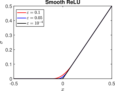
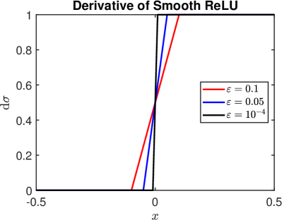
Figure 1: Smooth ReLU and derivative for different values of $\varepsilon$.

It follows from (7) that

$${\widehat{\Phi}}({\boldsymbol{\xi}};{\boldsymbol{\theta}})=\phi_{L}({\boldsymbol{\xi}})=W_{L-1}\Big{(}\big{(}I+h(\sigma\circ\mathcal{K}_{{L-1}})\big{)}\circ\dots\circ\big{(}I+h(\sigma\circ\mathcal{K}_{{1}})\big{)}\circ\mathcal{K}_{0}\Big{)}({\boldsymbol{\xi}}),$$ (9)

where $\mathcal{K}_{j}({\bf y})=W_{j}\,{\bf y}+{\bf b}_{j},$ for all $j=0,\ldots,L-1$ and for any $\bf y$.

To this end, the following two critical questions naturally come to mind:

1. How well does $\widehat{\Phi}({\boldsymbol{\xi}};{\boldsymbol{\theta}})$ approximate $\Phi({\boldsymbol{\xi}})$?

2. How do we determine ${\boldsymbol{\theta}}$?

We will address (b) first and leave (a) for a discussion provided in section 3.3. Now, setting ${\boldsymbol{\theta}}=\{W_{j},{\bf b}_{j}\},$ it follows that the problem of approximating $\Phi$ via ResNet is essentially the problem of learning the unknown parameter ${\boldsymbol{\theta}}.$ More specifically, the learning problem is the solution of the minimization problem [28]:

$$\min_{{\boldsymbol{\theta}}}\mathcal{J({\boldsymbol{\theta}};{\boldsymbol{\xi}},{\bf{u}})}$$ (10)

subject to constraints (7), where $\mathcal{J({\boldsymbol{\theta}},{\boldsymbol{\xi}},{\bf{u}})}$ is suitable loss function.

In this work, we consider the mean squared error, together with a regularization term, as our loss functional:

$$\mathcal{J}({\boldsymbol{\theta}};{\boldsymbol{\xi}},{\bf{u}})=\frac{1}{2N_{s}}\sum_{j=1}^{N_{s}}\|\hat{\Phi}({\boldsymbol{\xi}}_{j};{\boldsymbol{\theta}})-{\bf{u}}_{j}\|^{2}_{2}+\frac{\lambda}{2}||{\boldsymbol{\theta}}||_{2}^{2},$$ (11)

where $\lambda$ is the regularization parameter. Due to its highly non-convex nature, this is a very difficult optimization problem. Indeed, a search over a high dimensional parameter space for the global minimum of a non-convex function can be intractable. The current state-of-the-art approaches to solve these optimization problems are based on the stochastic gradient descent method [41, 49, 54].

As pointed out in, for instance, [28], the middle equation in expression (7) mimics the forward Euler discretization of a nonlinear differential equation:

$$d_{t}\phi(t) = \sigma(W(t)\phi(t)+b(t)),\;\;t\in(0,T],$$

$$\phi(0) = \phi_{0}.$$

It is known that standard DNNs are prone to vanishing gradient problem [50], leading to loss of information during the training phase. ResNets do help, but more helpful is the so-called DenseNet [35]. Notice that in a typical DenseNet, each layer takes into account all the previous layers. However, this is an ad hoc approach with no rigorous mathematical framework. Recently in [2], a mathematically rigorous approach based on fractional derivatives has been introduced. This ResNet is called Fractional DNN. In [2], the authors numerically establish that fractional derivative based ResNet outperforms ResNet in overcoming the vanishing gradient problem. This is not surprising because fractional derivatives allow connectivity among all the layers. Building rigorously on the idea of [2], we proceed to present the fractional DNN surrogate model for the discrete PDE in (1).

3.2 Fractional deep neural network

As pointed out in the previous section, the fractional DNN approach is based on the replacement of the standard ODE constraint in the learning problem by a fractional differential equation. To this end, we first introduce the definitions and concepts on which we shall rely to discuss fractional DNN.

Let $u:[0,T]\rightarrow\mathbb{R}$ be an absolutely continuous function and assume $\gamma\in(0,1)$. Next, consider the following fractional differential equations

$$d_{t}^{\gamma}u(t)=f(u(t)),\quad u(0)=u_{0},$$ (12)

and

$$d_{T-t}^{\gamma}u(t)=f(u(t)),\quad u(T)=u_{T}.$$ (13)

Here, $d_{t}^{\gamma}$ and $d_{T-t}^{\gamma}$ denote left and right Caputo derivatives, respectively [2].

Then, setting $u(t_{j})=u_{j},$ and using the $L^{1}$-scheme (see e.g., [2]) for the discretization of (12) and (13) yields, respectively,

$$u_{j+1}=u_{j}-\sum_{k=0}^{j-1}a_{j-k}\>\left(u_{k+1}-u_{k}\right)+h^{\gamma}\Gamma(2-\gamma)f(u_{j}),\quad j=0,...,L-1,\;$$ (14)

and

$$u_{j-1}=u_{j}+\sum_{k=j}^{L-1}a_{k-j}\>\left(u_{k+1}-u_{k}\right)-h^{\gamma}\Gamma(2-\gamma)f(u_{j}),\quad j=L,...,1,$$ (15)

where $h>0$ is the step size, $\Gamma(\cdot)$ is the Euler-Gamma function, and

$$a_{j-k}=(j+1-k)^{1-\gamma}-(j-k)^{1-\gamma}.$$ (16)

After this brief overview of the fractional derivatives, we are ready to introduce our fractional DNN (cf. (7))

$$\phi_{1} =\sigma(W_{0}\phi_{0}+{\bf b}_{0});\quad\phi_{0}={\boldsymbol{\xi}},$$

$$\phi_{j} =\phi_{j-1}-\sum_{k=0}^{j-2}a_{j-1-k}\>\left(\phi_{k+1}-\phi_{k}\right)+h^{\gamma}\Gamma(2-\gamma) \sigma(W_{j-1}\phi_{j-1}+{\bf b}_{j-1}),$$ (17)

$$2\leq j\leq L-1,$$

$$\phi_{L} =W_{L-1}\phi_{L-1}.$$

Our learning problem then amounts to

$$\min_{{\boldsymbol{\theta}}}\mathcal{J}({\boldsymbol{\theta}};{\boldsymbol{\xi}},{\bf{u}})$$ (18)

subject to constraints (3.2). Notice that the middle equation in (3.2) mimics the $L^{1}$-in time discretization of the following nonlinear fractional differential equation

$$d_{t}^{\gamma}\phi(t) =\sigma(W(t)\phi(t)+b(t)),\;\;t\in(0,T],$$

$$\phi(0) =\phi_{0}.$$

There are two ways to approach the constrained optimization problem (18). The first approach is the so-called reduced approach, where we eliminate the constraints (3.2) and consider the minimization problem (18) only in terms of ${\boldsymbol{\theta}}$. The resulting problem can be solved by using a gradient based method such as BFGS, see e.g., [38, Chapter 4]. During every step of the gradient method, one needs to solve the state equation (3.2) and an adjoint equation. These two solves enable us to derive an expression of the gradient of the reduced loss function with respect to ${\boldsymbol{\theta}}$. Alternatively, one can derive the gradient and adjoint equations by using the Lagrangian approach. It is well-known that the gradient with respect to ${\boldsymbol{\theta}}$ for both approaches coincides, see [3, pg. 14] for instance. We next illustrate how to evaluate this gradient using the Lagrangian approach.

The Lagrangian functional associated with the discrete constrained optimization problem (18) is given by

$$\mathcal{L}({\bf{u}},{\boldsymbol{\theta}},\boldsymbol{\psi}):=\mathcal{J({\boldsymbol{\theta}};{\boldsymbol{\xi}},{\bf{u}})}+\langle\phi_{1}-\sigma(W_{0}\phi_{0}+{\bf b}_{0}),\psi_{1}\rangle\\ +\sum_{j=2}^{L-1}\Bigg{\langle}\phi_{j}-\phi_{j-1}+\sum_{k=0}^{j-2}a_{j-1-k}\>\left(\phi_{k+1}-\phi_{k}\right)+h^{\gamma}\Gamma(2-\gamma)\sigma(W_{j-1}\phi_{j-1}+{\bf b}_{j-1}),\psi_{j}\Bigg{\rangle}\\ +\langle\phi_{L}-W_{L-1}\phi_{L-1},\psi_{L}\rangle,$$ (19)

where $\psi_{j}$’s are the Lagrange multi1pliers, also called adjoint variables, corresponding to (3.2) and $\langle\cdot,\cdot\rangle$ is the inner product on $\mathbb{R}^{N_{x}}$.

Next we write the state and adjoint equations fulfilled at a stationary point of the Lagrangian $\mathcal{L}$. In addition, we state the derivative of $\mathcal{L}$ with respect to the design variable ${\boldsymbol{\theta}}$.

1. State Equation.

   $$\begin{aligned} \phi_{1}&=\sigma(W_{0}{{\boldsymbol{\xi}}}+{\bf b}_{0}),\\ \phi_{j}&=\phi_{j-1}-\sum_{k=0}^{j-2}a_{j-1-k}\>\left(\phi_{k+1}-\phi_{k}\right)+h^{\gamma}\Gamma(2-\gamma)\sigma(W_{j-1}\phi_{j-1}+{\bf b}_{j-1}),\\ &\hskip 227.62204pt2\leq j\leq L-1,\\ \phi_{L}&=W_{L-1}\phi_{L-1}.\end{aligned}$$ (20a)

2. Adjoint Equation.

   $$\psi_{j} =\psi_{j+1}+\sum_{k=j+1}^{L-2}a_{k-j}\>\left(\psi_{k+1}-\psi_{k}\right)-\hskip 28.45274ptj=L-2,...,1$$ (20b)

   $$\hskip 71.13188pth^{\gamma}\Gamma(2-\gamma)\left[-W_{j}^{T}\left(\psi_{j+1}\odot\sigma^{\prime}\left(W_{j}\phi_{j+1}+{\bf b}_{j}\right)\right)\right],$$

   $$\psi_{L-1} =-W_{L-1}^{T}\psi_{L},$$

   $$\psi_{L} =\partial_{\phi_{L}}\mathcal{J({\boldsymbol{\theta}};{\boldsymbol{\xi}},{\bf{u}})}.$$

3. Derivative with respect to ${\boldsymbol{\theta}}$.

   $$\partial_{W_{L-1}}\mathcal{L} =\psi_{L}\;\phi_{L-1}^{T}=\partial_{\phi_{L}}\mathcal{J({\boldsymbol{\theta}};{\boldsymbol{\xi}},{\bf{u}})}\;\phi_{L-1}^{T},$$ (20c)

   $$\partial_{W_{j}}\mathcal{L}= -\phi_{j}\>\left(\psi_{j+1}\odot\sigma^{\prime}(W_{j}\phi_{j}+{\bf b}_{j})\right)^{T}+\partial_{W_{j}}\mathcal{J({\boldsymbol{\theta}};{\boldsymbol{\xi}},{\bf{u}})},$$

   $$\hskip 156.49014ptj=0,...,L-2,$$

   $$\partial_{{\bf b}_{j}}\mathcal{L}= -\;\psi_{j+1}^{T}\;\sigma^{\prime}(W_{j}\phi_{j}+{\bf b}_{j})+\partial_{{\bf b}_{j}}\mathcal{J({\boldsymbol{\theta}};{\boldsymbol{\xi}},{\bf{u}})}.$$

   $$\hskip 156.49014ptj=0,...,L-2\,.$$

The right-hand-side of (20c) represents the gradient of $\mathcal{L}$ with respect to ${\boldsymbol{\theta}}$. We then use a gradient-based method (BFGS in our case) to identify ${\boldsymbol{\theta}}$.

3.3 Error analysis

In this section we briefly address the question of how well the deep neural approximation approximates the PDE solution map $\Phi:\mathbb{R}^{N_{{\boldsymbol{\xi}}}}\rightarrow\mathbb{R}^{N_{x}}.$ The approximation capabilities of neural networks has received a lot of attention recently in the literature, see e.g., [15, 34, 46, 53] and the references therein. The papers [34, 46] obtain results based on general activation functions for which the approximation rate is $\mathcal{O}(n^{-1/2})$, where $n$ is the total number of hidden neurons. This implies that neural networks can overcome the curse of dimensionality, as the approximation rate is independent of dimension $N_{x}$.

We begin by making the observation that the fractional DNN can be written as a linear combination of activation functions evaluated at different layers. Indeed, observe from (3.2) that if $\Phi({\boldsymbol{\xi}})$ is approximated by a one-hidden layer network $\hat{\Phi}({\boldsymbol{\xi}},{\boldsymbol{\theta}}):=\phi_{2}$ (that is, $L=2$) then it can be expressed as:

$$\phi_{2}=W_{1}\sigma(W_{0}{\boldsymbol{\xi}}+{\bf b}_{0}).$$ (21)

By a one-hidden layer network, we mean a network with the input layer, one hidden layer and the output layer [15, 34, 39, 46]. Next, for $L=3$, we obtain

$$\phi_{3}=W_{2}\phi_{2}=W_{2}\left[\alpha_{0}\sigma(W_{0}\phi_{0}+{\bf b}_{0})+\alpha_{1}\sigma(W_{1}\phi_{1}+{\bf b}_{1})+\alpha_{2}\phi_{0}\right],$$ (22)

where $\alpha_{0}=1-a_{1},\;\alpha_{1}=\tau:=h^{\gamma}\Gamma(2-\gamma)$ and $\alpha_{2}=a_{1}.$ Similarly, if we set $L=4$, then we get

$$\phi_{4} = W_{3}\phi_{3}$$ (23)

$$= W_{3}\left[\alpha_{0}\sigma(W_{0}\phi_{0}+{\bf b}_{0})+\alpha_{1}\sigma(W_{1}\phi_{1}+{\bf b}_{1})+\alpha_{2}\sigma(W_{2}\phi_{2}+{\bf b}_{2})+\alpha_{3}\phi_{0}\right],$$

where $\alpha_{0}=(1-a_{1}+a_{1}^{2}-a_{2}),\;\alpha_{1}=(1-a_{1})\tau,\;\alpha_{2}=\tau,$ and $\alpha_{3}=2a_{2}-a_{1}-a_{1}^{2}.$

Proceeding in a similar fashion yields the following result regarding multilayer fractional DNN.

Proposition 1 (Representation of multilayer fractional DNN).

For $L\geq 3$, the fractional DNN given by (3.2) fulfills

$$\phi_{L}=W_{L-1}\left[\alpha_{L-1}\phi_{0}+\sum_{i=0}^{L-2}\alpha_{i}\sigma(W_{i}\phi_{i}+{\bf b}_{i})\right],$$ (24)

where $\alpha_{i}$ are constants depending on $\tau$ and $a_{i}$, as given by (16). Observe that a one-hidden layer fDNN (that is, $L=2$) coincides with a one-hidden layer standard DNN.

Error analysis for multilayer networks is generally challenging. Some papers that study this include [30, 53] and the references therein. The results of these two papers focus mainly on the ReLU activation function. In particular, [30] discusses the approximation of linear finite elements by ReLU deep and shallow networks.

In this paper, we restrict the analysis discussion to one-hidden layer fDNN i.e., $L=2$. In particular, we consider a one-hidden layer network with finitely many neurons. Notice that for $L=2$, fDNN coincides with standard DNN according to Proposition 1. Therefore, it is possible to extend the result from [46] to our case. To state the result from [46], we first introduce some notation.

To this end, we make the assumption that the function $\Phi({\boldsymbol{\xi}})$ is defined on a bounded domain $\mathcal{P}\subset\mathbb{R}^{N_{{\boldsymbol{\xi}}}}$ and has a bounded Barron norm

$$||\Phi||_{\mathcal{B}^{m}}=\int_{\mathcal{P}}(1+\omega)^{m}|\hat{\Phi}(\omega)|\;d\omega,\;\;m\geq 0.$$ (25)

Now, let $m\in\mathbb{N}\cup\{0\}$ and $p\in[1,\infty].$ Recall that the Sobolev space $\mathcal{W}^{m,p}(\mathcal{P})$ is the space of functions in $L^{p}(\mathcal{P})$ whose weak derivatives of order $m$ are also in $L^{p}(\mathcal{P}):$

$$\mathcal{W}^{m,p}(\mathcal{P}):=\{f\in L^{p}(\mathcal{P}):D^{\bf m}f\in L^{p}(\mathcal{P}),\;\forall{\bf m}\;\mbox{with}\;|{\bf m}|\leq m\},$$ (26)

where ${\bf m}=(m_{1},\ldots,m_{N_{\xi}})\in\{0,1,\ldots\}^{N_{\xi}},$ $|{\bf m}|=m_{1}+m_{2}\ldots+m_{N_{\xi}}$ and $D^{\bf m}f$ is the weak derivative. In particular, the space $\mathcal{H}^{m}(\mathcal{P}):=\mathcal{W}^{m,2}(\mathcal{P})$ is a Hilbert space with inner product and norm given respectively by

$$(f,g)_{\mathcal{H}^{m}(\mathcal{P})}=\sum_{|{\bf m}|\leq m}\int_{\mathcal{P}}D^{\bf m}f({\bf x})D^{\bf m}g({\bf x})\;d{\bf x},$$

and $||f||_{\mathcal{H}^{m}(\mathcal{P})}=(f,f)^{1/2}_{\mathcal{H}^{m}(\mathcal{P})}.$ For $p=\infty,$ we note that the Sobolev space $\mathcal{W}^{m,\infty}(\mathcal{P})$ is equipped with the norm

$$||f||_{\mathcal{W}^{m,\infty}(\mathcal{P})}=\max_{{\bf m}:|{\bf m}|\leq m}\mbox{ess}\sup_{{\bf x}\in\mathcal{P}}|D^{\bf m}f({\bf x})|.$$ (27)

Also, we say that $f\in\mathcal{W}_{loc}^{m,p}(\mathcal{P})$ if $f\in\mathcal{W}^{m,p}(\mathcal{P}^{\prime}),\;\;\forall$ compact ${\mathcal{P}^{\prime}}\subset\mathcal{P}.$

Next, since the mapping $\Phi:\mathbb{R}^{N_{{\boldsymbol{\xi}}}}\rightarrow\mathbb{R}^{N_{x}}$ can be computed using ${N_{x}}$ mappings $\Phi_{j}:\mathbb{R}^{N_{{\boldsymbol{\xi}}}}\rightarrow\mathbb{R},$ it suffices to focus on networks with one output unit. Observe from (21) that

$$\hat{\Phi}({\boldsymbol{\xi}},{\boldsymbol{\theta}}):=\phi_{2}=\sum_{i=1}^{n}c_{i}\cdot\sigma(\omega_{i}\cdot\xi+b_{i}),$$ (28)

where $n$ is the total number of neurons in the hidden layer, $b_{i}$ an element of the bias vector, $c_{i}$ and $\omega_{i}$ are rows of $W_{1}$ and $W_{0}$ respectively. Now, for a given activation function $\sigma,$ define the set

$$\mathcal{F}_{N_{{\boldsymbol{\xi}}}}^{n}(\sigma)=\left\{\sum_{i=1}^{n}c_{i}\cdot\sigma(\omega_{i}\cdot\xi+b_{i}),\quad\omega_{i}\in\mathbb{R}^{N_{\xi}},\;b_{i}\in\mathbb{R}\right\}.$$ (29)

We can now state the following result for any non-zero activation functions satisfying some regularity conditions [46, Corollary 1]. After this result, we will show that our activation function in (8) fulfills the required assumptions.

Theorem 2.

Let $\mathcal{P}$ be a bounded domain and $\sigma\in\mathcal{W}_{loc}^{m,\infty}(\mathbb{R})$ be a non-zero activation function. Suppose there exists a function $\nu\in\mathcal{F}_{1}^{q}(\sigma)$ satisfying

$$|\nu^{(k)}(t)|\leq C_{p}(1+|t|)^{-p},\;\;0\leq k\leq m,\;\;p>1.$$ (30)

Then, for any $\Phi\in\mathcal{B}^{m},$ we have

$$\inf_{\hat{\Phi}_{n}\in\mathcal{F}_{N_{\xi}}^{n}(\sigma)}||\Phi-\hat{\Phi}_{n}||_{\mathcal{H}^{m}(\mathcal{P})}\leq C(\sigma,m,p,\beta)|\mathcal{P}|^{1/2}{q}^{1/2}n^{-1/2}||\Phi||_{\mathcal{B}^{m+1}},$$ (31)

where $\beta=\mbox{diam}(\mathcal{P})$ and $C$ is a constant depending on $\sigma,m,p$ and $\beta.$

Note that the bound in (31) is $\mathcal{O}(n^{-1/2}).$ Here, the function $\nu(x)$ is a linear combination of the shifts and dilations of the activation $\sigma(x).$ Moreover, the activation function itself need not satisfy the decay (30). The theorem says that it suffices to find some function $\nu\in\mathcal{F}_{1}^{q}(\sigma)$ (cf. (29) with $n=q,\;N_{\xi}=1$) for which (30) holds.

In this paper, we are working with smooth ReLU (see (8)) as the activation function $\sigma(x)$ for which $m=2$. One choice of $\nu$ for which (30) holds is $\nu\in\mathcal{F}_{1}^{3}(\sigma)$ given by

$$\nu(t)=\sigma(t+1)+\sigma(t-1)-2\sigma(t).$$ (32)

It can be shown that, $\nu$ satisfies (30) with $C_{p}=20$ and $p=1.5$, that is,

$$|\nu^{(k)}(t)|\leq 20(1+|t|)^{-1.5},\;\;0\leq k\leq 2.$$ (33)

This can be verified from Figure 2.

Figure 2: Verification of the decay condition (30) for $\nu$ in (32), which has been defined using the smooth ReLU in (8).

In what follows, we discuss the application of our proposed fractional DNN to the solution of two statistical Bayesian inverse problems.

4 Application to Bayesian inverse problems

The inverse problem associated with the forward problem (1) essentially requires estimating a parameter vector ${\boldsymbol{\xi}}\in\mathbb{R}^{N_{{\boldsymbol{\xi}}}}$ given some observed noisy limited data $d\in\mathbb{R}^{N_{x}}.$ In the Bayesian inference framework, the posterior probability density, $\pi({\boldsymbol{\xi}}|d):\mathbb{R}^{N_{{\boldsymbol{\xi}}}}\rightarrow\mathbb{R},$ solves the statistical inverse problem. In principle, $\pi({\boldsymbol{\xi}}|d)$ encodes the uncertainty from the set of observed data and the sought parameter vector. More formally, the posterior probability density is given by Baye’s rule as

$$\pi_{pos}({\boldsymbol{\xi}}):=\pi({\boldsymbol{\xi}}|d)\propto\pi({\boldsymbol{\xi}})\pi(d|{\boldsymbol{\xi}}),$$ (34)

where $\pi(\cdot):\mathbb{R}^{N_{{\boldsymbol{\xi}}}}\rightarrow\mathbb{R}$ is the prior and $\pi(d|{\boldsymbol{\xi}})$ is the likelihood function. The standard approach to Bayesian inference uses the assumption that the observed data are of the form (see e.g., [10, 20])

$$d=\Phi({\boldsymbol{\xi}})+\eta,$$ (35)

where $\Phi$ is the parameter-to-observable map and $\eta\sim\mathcal{N}(0,\Sigma_{\eta})$. In our numerical experiments, we assume that $\Sigma_{\eta}=\kappa^{2}I,$ where $I$ is the identity matrix with appropriate dimensions and $\kappa$ denotes the variance. Now, let the log-likelihood be given by

$$L({\boldsymbol{\xi}})=\frac{1}{2}\left|\left|\Sigma_{\eta}^{1/2}(d-\Phi({\boldsymbol{\xi}}))\right|\right|^{2};$$ (36)

then Baye’s rule in (34) becomes

$$\pi_{pos}({\boldsymbol{\xi}}):=\pi({\boldsymbol{\xi}}|d)\propto\pi({\boldsymbol{\xi}})\pi(d|{\boldsymbol{\xi}})=\frac{1}{Z}\exp\left(-L({\boldsymbol{\xi}})\right)\pi({\boldsymbol{\xi}}),$$ (37)

where $Z=\int_{\mathcal{P}}\exp(-L({\boldsymbol{\xi}}))\pi({\boldsymbol{\xi}})\;d{\boldsymbol{\xi}}$ is a normalizing constant.

We note here that, in practice, the posterior density rarely admits analytic expression. Indeed, it is generally evaluated using Markov chain Monte Carlo (MCMC) sampling techniques. In MCMC schemes one has to perform several thousands of forward model simulations. This is a significant computational challenge, especially if the forward model represents large-scale high fidelity discretization of a nonlinear PDE. It is therefore reasonable to construct a cheap-to-evaluate surrogate for the forward model in the offline stage for use in online computations in MCMC algorithms.

In what follows, we discuss MCMC schemes for sampling posterior probability distributions, as well as how our fractional DNN surrogate modeling strategy can be incorporated in them.

4.1 Markov Chain Monte Carlo

Markov chain Monte Carlo (MCMC) methods are very powerful and flexible numerical sampling approaches for approximating posterior distributions, see e.g., [8, 10, 47]. Prominent MCMC methods include Metropolis-Hastings algorithm (MH) [47], Gibbs algorithm [5] and Hamiltonian Monte Carlo algorithm (HMC) [8, 9], Metropolis-adjusted Langevin algorithm (MALA) [8], and preconditioned Crank Nicolson algorithm (pCN) [5], and their variants. In our numerical experiments, we will use MH, pCN, HMC, and MALA algorithms. We will describe only MH in this paper and refer the reader to [8] for the details of the derivation and properties of the many variants of the other three algorithms.

To this end, consider a given parameter sample ${\boldsymbol{\xi}}={\boldsymbol{\xi}}^{i}$. The MH algorithm generates a new sample ${\boldsymbol{\xi}}^{i+1}$ as follows:

1. Generate a proposed sample ${\boldsymbol{\xi}}^{\ast}$ from a proposal density $q({\boldsymbol{\xi}}^{\ast}|{\boldsymbol{\xi}})$, and compute $q({\boldsymbol{\xi}}|{\boldsymbol{\xi}}^{\ast})$.

2. Compute the acceptance probability

   $$\alpha({\boldsymbol{\xi}}^{\ast}|{\boldsymbol{\xi}})=\min\left\{1,\frac{\pi({\boldsymbol{\xi}}^{\ast}|d)q({\boldsymbol{\xi}}^{\ast}|{\boldsymbol{\xi}})}{\pi({\boldsymbol{\xi}}|d)q({\boldsymbol{\xi}}|{\boldsymbol{\xi}}^{\ast})}\right\}.$$ (38)

3. If $\mbox{Uniform}(0;1]<\alpha({\boldsymbol{\xi}}^{\ast}|{\boldsymbol{\xi}}),$ then ${\boldsymbol{\xi}}^{i+1}={\boldsymbol{\xi}}^{\ast}.$ Else, set ${\boldsymbol{\xi}}^{i+1}={\boldsymbol{\xi}}$.

Observe from (36) and (37) that each evaluation of the likelihood function, and hence, the acceptance probability (38) requires the evaluation of the forward model to compute $\pi({\boldsymbol{\xi}}^{\ast}|d)$. In practice, one has to do tens of thousands of forward solves for the HM algorithm to converge. We propose to replace the forward solves by the fractional DNN surrogate model. In our numerical experiments, we follow [27] in which an adaptive Gaussian proposal is used:

$$q({\boldsymbol{\xi}}^{\ast}|{\boldsymbol{\xi}}^{i})=\exp\left(-\frac{1}{2}({\boldsymbol{\xi}}^{\ast}-{\boldsymbol{\xi}}^{i-1})^{T}C_{i-1}({\boldsymbol{\xi}}^{\ast}-{\boldsymbol{\xi}}^{i-1})\right),$$ (39)

where $C_{0}=I,$

$$C_{i-1}=\frac{1}{i}\sum_{j=0}^{i-1}({\boldsymbol{\xi}}^{j}-\bar{\boldsymbol{\xi}})({\boldsymbol{\xi}}^{j}-\bar{\boldsymbol{\xi}})^{T}+\vartheta I,$$

$\bar{\boldsymbol{\xi}}=i^{-1}\sum_{j=0}^{i-1}{\boldsymbol{\xi}}^{j},$ and $\vartheta\approx 10^{-8}.$ When the proposal is chosen adaptively as specified above, the HM method is referred to as an Adaptive Metropolis (AM) method [4, 27].

5 Numerical Experiments

In this section, we consider two statistical inverse problems. The first one is a diffusion-reaction problem in which two parameters need to be inferred [18]. The second one is a more challenging problem – a thermal fin problem from [8], which involves one hundred parameters to be identified. All experiments were performed using MATLAB R2020b on a Mac desktop with RAM 32GB and CPU 3.6 GHz Quad-Core Intel Core i7.

In both of these experiments we train using a 3-hidden layer network with $15$ neurons in each hidden layer (that is, $L=4,\;n=45$) and $k=400$ neurons in the output layer, where $k$ matches the dimension of POD basis as described in section 5.1 below. We chose $\varepsilon=0.1$ in the smooth ReLU activation function, final time $T=1$ and step-size $h=\frac{1}{3}$. We set the fractional exponent $\gamma=0.5$ in the Caputo Fractional derivative and the regularization parameter $\lambda=10^{-6}$. To train the network, we use the BFGS optimization method [38, Chapter 4].

Tables 1 and 2 show the number of BFGS iterations and the CPU times required to train the data from the diffusion-reaction problem and the thermal fin problem, respectively. Also shown in these tables are the relative errors obtained by evaluating the trained network at a parameter ${\boldsymbol{\xi}}^{e}$ not in the training set $\mathbb{E}$; here,

$$Error=\frac{||u({\boldsymbol{\xi}}^{e})-\hat{\Phi}({\boldsymbol{\xi}}^{e})||_{\infty}}{||u({\boldsymbol{\xi}}^{e})||_{\infty}},$$

where $u({\boldsymbol{\xi}}^{e})$ and $\hat{\Phi}({\boldsymbol{\xi}}^{e})$ are the true and surrogate solutions at ${\boldsymbol{\xi}}^{e}$, respectively. Note from both tables that after $1600$ BFGS iterations, the decrease in errors is not significant. Hence, for all the experiments discussed below, we use $1600$ BFGS iterations.

BFGS iterations	Error	Time (in sec)
$400$	$2.26\times 10^{-2}$	$7.99$
$800$	$1.10\times 10^{-2}$	$15.10$
$1600$	$4.09\times 10^{-3}$	$29.45$
$3200$	$3.43\times 10^{-3}$	$56.14$
$6400$	$2.56\times 10^{-3}$	$105.66$

Table 1: Diffusion-reaction problem: Number of BFGS iterations, relative errors and times for training the fractional DNN.

BFGS iterations	Error	Time (in sec)
$400$	$1.87\times 10^{-2}$	$10.69$
$800$	$1.15\times 10^{-2}$	$18.51$
$1600$	$7.39\times 10^{-3}$	$33.52$
$3200$	$4.80\times 10^{-3}$	$62.90$
$6400$	$3.73\times 10^{-3}$	$117.55$

Table 2: Thermal fin problem: Number of BFGS iterations, relative errors and times for training the fractional DNN.

5.1 Diffusion-reaction example

We consider the following nonlinear diffusion-reaction problem posed in a two-dimensional spatial domain [11, 24]

$$\begin{aligned} -\Delta u+g(u;{\boldsymbol{\xi}})&=f,\quad\mbox{in }\Omega=(0,1)^{2},\\ u&=0,\quad\mbox{on }\partial\Omega,\end{aligned}$$ (40)

where $g(u;{\boldsymbol{\xi}})=\frac{{\boldsymbol{\xi}}_{2}}{{\boldsymbol{\xi}}_{1}}\left[\exp({\boldsymbol{\xi}}_{1}u)-1\right]$ and $f=100\sin(2\pi x_{1})\sin(2\pi x_{2})$. Moreover, the parameters are ${\boldsymbol{\xi}}=({\boldsymbol{\xi}}_{1},{\boldsymbol{\xi}}_{2})\in[0.01,10]^{2}\subset\mathbb{R}^{2}$.

Equation (40) is discretized on a uniform mesh in $\Omega$ with $64$ grid points in each direction using centered differences resulting in $4096$ degrees of freedom. We obtained the solution of the resulting system of nonlinear equations using an inexact Newton-GMRES method as described in [37]. The stopping tolerance was $10^{-6}.$

To train the network, we first computed $N_{s}=900$ solution snapshots $\mathbb{S}$ corresponding to a set $\mathbb{E}$ of $900$ parameters ${\boldsymbol{\xi}}=({\boldsymbol{\xi}}_{1},{\boldsymbol{\xi}}_{2})$ drawn from the parameter space $[0.01,10]^{2}$. These parameters were chosen using Latin hypercube sampling. Each solution snapshot is of dimension $N_{x}=4096.$ Next, we computed the SVD of the matrix of solution snapshots $\mathbb{S}=\widetilde{\mathbb{V}}\Sigma\mathbb{W}^{T},$ and set our POD basis $\mathbb{V}=\widetilde{\mathbb{V}}(:,1:k),$ where $k=400.$ Our training set then consisted of $\mathbb{E}$ as inputs and $\mathbb{V}^{T}\mathbb{S}\in\mathbb{R}^{k\times N_{s}}$ as our targets. As reported by Hesthaven and Ubbiali in [32] in the context of solving parameterized PDEs, the POD-DNN approach accelerates the online computations for surrogate models. Thus, we follow this approach in our numerical experiments; in particular, using $k$-dimensional data (where $k\ll N_{x}$) confirms an overall speed up in the solution of the statistical inverse problems.

Next, in both numerical examples considered in this paper, we solved the inverse problems using $M=20,000$ MCMC samples. In each case, the first $10,000$ samples were discarded for “burn-in” effects, and the remaining $10,000$ samples were used to obtain the reported statistics. Here, we used an initial Gaussian proposal (39) with covariance $C_{0}=I$ and updated the covariance after every $100$th sample. As in [18], we assume for this problem, that ${\boldsymbol{\xi}}$ is uniformly distributed over the parameter space $[0.01,10]^{2}$. Hence, (37) becomes

$$\pi_{pos}({\boldsymbol{\xi}}) \propto\begin{cases}\exp\left(-\frac{1}{2\kappa^{2}}(d-\Phi({\boldsymbol{\xi}}))^{T}(d-\Phi({\boldsymbol{\xi}}))\right)&\text{if }{\boldsymbol{\xi}}\in[0.01,10]^{2}.\\ 0&\text{otherwise.}\end{cases}$$ (41)

We generated the observations $d$ by using (35) the true parameter to be identified ${\boldsymbol{\xi}}^{e}=(1,0.1)$ and a Gaussian noise vector $\eta$ with $\kappa=10^{-2}.$

Figures 3, 4 and 5, represent, respectively, the histogram (which depicts the posterior distribution), the Markov chains and the autocorrelation functions corresponding to the parameters using the high fidelity model (Full) and the deep neural network surrogate (DNN) models in the MCMC algorithm. Recall that, for a Markov chain $\{\delta_{j}\}_{j=1}^{J}$ generated by the Metropolis-Hastings algorithm, with variance $\kappa^{2},$ the autocorrelation function (ACF) $\varrho$ of the $\delta$-chain is given by

$$\varrho(j)=\mbox{cov}(\delta_{1},\delta_{1+|j|})/\kappa^{2}.$$

and the integrated autocorrelation time, $\tau_{int}$, (IACT) of the chain is defined as

$$\tau_{int}(\delta) := \sum_{j=-J+1}^{J-1}\varrho(j)\approx 1+2\sum_{j=1}^{J-1}\left(1-\frac{j}{J}\right)\mbox{cov}(\delta_{1},\delta_{1+j})/\kappa^{2}.$$ (42)

ACF decays very fast to zero as $J\rightarrow\infty.$ In parctice, $J$ is often taken to be $\left\lfloor{10\log_{10}M}\right\rfloor,$ [5]. If $\mbox{IACT}=K,$ this means that the roughly every $K$th sample of the $\delta$ chain is independent. We have used the following estimators to approximate $\varrho(j)$ and $\tau_{int}$ in our computations [4, 48]:

$$\varrho(j):=B(j)/B(0),\;\;\mbox{and}\;\;\tau_{int}:=\sum_{j=-\widehat{J}}^{\widehat{J}}\varrho(j),$$

where $B(j)=\frac{1}{J-j}\sum_{k=1}^{J-j}(\delta_{k}-\bar{\delta})(\delta_{k+|j|}-\bar{\delta}),$ $\bar{\delta}$ is the mean of the $\delta$-chain, and ${\widehat{J}}$ is chosen be the smallest integer such that ${\widehat{J}}\geq 3\tau_{int}.$

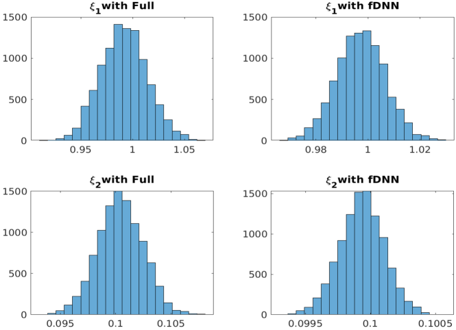
Figure 3: Histograms of the posterior distributions for the parameters ${\boldsymbol{\xi}}=({\boldsymbol{\xi}}_{1},{\boldsymbol{\xi}}_{2}).$ They have been obtained from Full (left) and fDNN (right) models with $M=10,000$ MCMC samples.

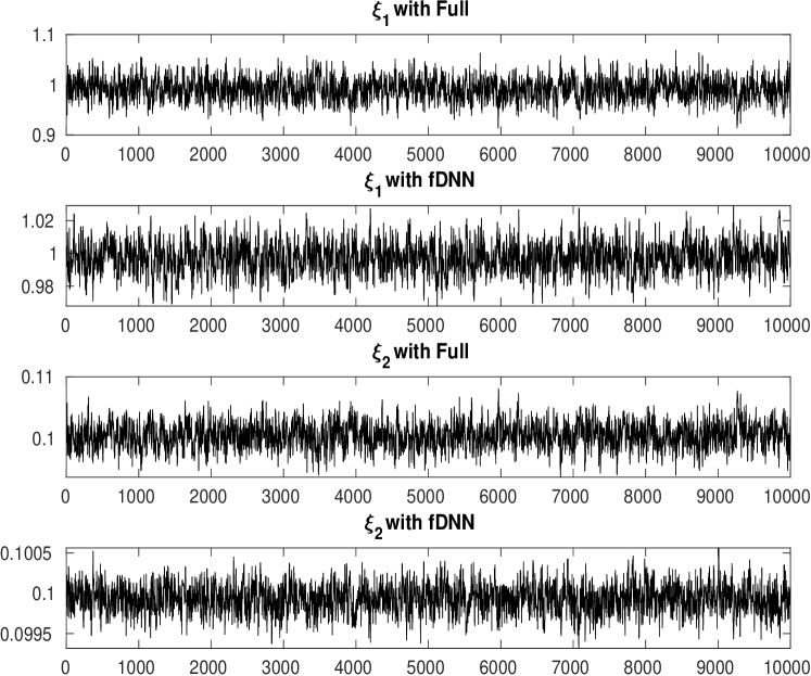
Figure 4: MCMC samples for the parameters ${\boldsymbol{\xi}}=({\boldsymbol{\xi}}_{1},{\boldsymbol{\xi}}_{2})$ using Full (first and third) and fDNN (second and fourth) models. For the full model, the $95\%$ confidence interval for $\xi_{1}$ and $\xi_{2}$ are $[0.9496,1.0492]$ and $[0.0954,0.1048]$. For the fDNN model, the $95\%$ confidence interval for $\xi_{1}$ and $\xi_{2}$ are $[0.9818,1.0196]$ and $[0.0995,0.1005]$.

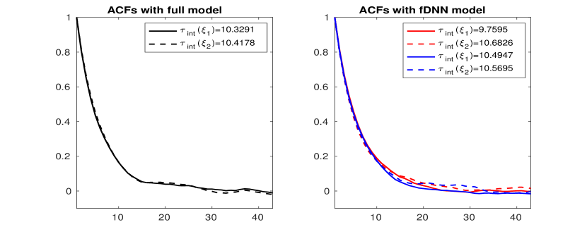
Figure 5: Autocorrelation functions (ACFs) for ${\boldsymbol{\xi}}_{1}$ and ${\boldsymbol{\xi}}_{2}$ chains computed with Full (left) and DNN (right) models. The red and blue lines are ACFs obtained with 1600 and 6400 BFGS iterations, respectively.

Observe from Figs. 3 and 4 that, for both Full and fDNN models, the respective histograms and Markov chains are centered around the parameters of interest $(1,0.1).$ In fact, for the full model, the $95\%$ confidence intervals (CIs) for $\xi_{1}$ and $\xi_{2}$ are $[0.9496,1.0492]$ and $[0.0954,0.1048]$. For the fDNN model, the CIs are $[0.9818,1.0196]$ and $[0.0995,0.1005]$. Thus, fDNN identifies $(1,0.1)$ appropriately.

We also examine the impact of training accuracy in Fig 5. The figure shows that the ACFs decay very fast to zero, as expected. The value of IACT is roughly $10$ for all the MCMC chains generated by the full model (left). The right of the figure shows the IACT for fDNN model, where the red-colored curves show the results obtained with $1600$ training steps and the blue curves show those obtained with $6400$ steps. In general, the IACT values imply that roughly every $10th$ sample of the MCMC chains generated by both the full and the fDNN models are independent.

These results indicate that the fDNN surrogate model produces results with accuracy comparable to those obtained using the full model. The advantage of the surrogate lies in its reduced costs. In this example, using the HM algorithm, the full model required $2347.7$ seconds of CPU time to solve the inverse problem, whereas the fractional DNN model required $29.3$ seconds (the online costs for fDNN), a reduction in CPU time of a factor of $80$. As always for surrogate approximations, there is overhead, the offline computations, associated with construction of the surrogate, i.e., identification of the parameter set ${\boldsymbol{\theta}}$ that defines the fDNN. For this example, this entailed construction of the $900$ snapshot solutions used to produce targets for the training process, computation of the SVD of the matrix $\mathbb{S}$ of snapshots giving the targets, together with the training of the network (using BFGS). The times required for these computations were $127.8$ seconds to construct the inputs/targets, $0.52$ second to compute the SVD and $29.5$ seconds to train the network. Thus, the offline and online times sum to $187.1$ seconds, which is a lot smaller than the time needed for the full solution (that is, $2347.7$ seconds). Of course, the offline computations represent a one-time expense which need not be repeated if more samples are used to perform an MCMC simulation or if different MCMC algorithms are used. This is, for instance, the case with the Differential Evolution Adaptive Metropolis (DREAM) method which runs multiple different chains simultaneously when used to sample the posterior distributions [51].

5.2 Thermal fin example

Next, we consider the following thermal fin problem from [8]:

$$\begin{aligned} -\mbox{div }(e^{{\boldsymbol{\xi}}({\bf x})}\nabla u)&=0,\quad&&\mbox{in }\Omega,\\ (e^{{\boldsymbol{\xi}}({\bf x})}\nabla u)\cdot{\bf n}+0.1u&=0,\quad&&\mbox{on }\partial\Omega\setminus\Gamma,\,\\ (e^{{\boldsymbol{\xi}}({\bf x})}\nabla u({\bf x}))\cdot{\bf n}&=1,\quad&&\mbox{on }\Gamma=(-0.5,0.5)\times\{0\}.\end{aligned}$$ (43)

These equations (43) represent a forward model for heat conduction over the non-convex domain $\Omega$ as shown in Fig. 6. Given the heat conductivity function $e^{{\boldsymbol{\xi}}({\bf x})}$, the forward problem (43) is used to compute the temperature $u$. The goal of this inverse problem is to infer $100$ unknown parameters ${\boldsymbol{\xi}}$ from $262$ noisy observations of $u$. Fig. 6 shows the location of the observations on the boundary $\partial\Omega\setminus\Gamma$, as well as the forward PDE solution $u$ at the true parameter ${\boldsymbol{\xi}}$.

To train the network, we first computed, as in the diffusion-reaction case, $N_{s}=900$ solution snapshots $\mathbb{S}$ corresponding to $900$ parameters ${\boldsymbol{\xi}}\in\mathbb{R}^{100}$ drawn using Latin hypercube sampling. This problem is a lot more difficult than the previous problem in the sense that the dimension of the parameter space in this case is $100$ rather than $2.$ Next, we compute the SVD of $\mathbb{S}$ and proceed as before.

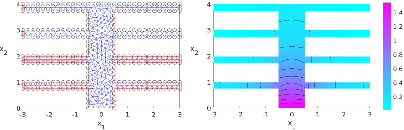
Figure 6: The location of observations (circles) (left) and the forward PDE solution $u$ under the true parameter ${\boldsymbol{\xi}}$ (right).

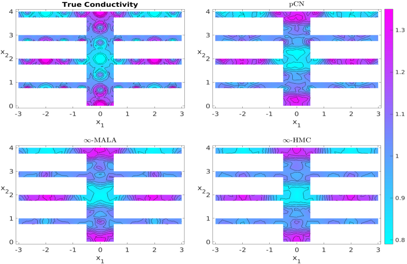
Figure 7: The true heat conductivity field $e^{{\boldsymbol{\xi}}({\bf x})}$ (upper left) and the mean estimates of the posterior obtained by the different MCMC methods using fractional DNN as a surrogate model.

In what follows, the infinite variants of Riemannian manifold Metropolis-adjusted Langevin algorithm (MALA) and Hamiltonian Monte-Carlo (HMC) algorithms as presented in [8] are denoted, respectively, by $\infty$-MALA and $\infty$-HMC. In particular, Fig. 7 shows the true conductivity, as well as the posterior mean estimates obtained by three MCMC methods – pCN, $\infty$-MALA and $\infty$-HMC – using the fractional DNN as a surrogate model.

As in [8], for this problem we used a Gaussian prior defined on the domain $\mathcal{D}:=[-3,3]\times[0,4]$ with covariance $\mathcal{C}$ of eigen-structure given by

$$\mathcal{C}=\sum_{i\in I}\mu_{i}^{2}\{\varphi_{i}\otimes\varphi_{i}\},$$

where $\mu_{i}^{2}=\{\pi^{2}((i_{1}+1/2)^{2}+(i_{2}+1/2)^{2})\}^{-1.2},$

$$\varphi_{i}({\bf x})=2|\mathcal{D}|^{-1/2}\cos(\pi(i_{1}+1/2)x_{1})\cos(\pi(i_{2}+1/2)x_{2}),$$

and $I=\{i=(i_{1},i_{2}),i_{1}\geq 0,\;i_{2}\geq 0\}.$ Moreover, the log-conductivity ${\boldsymbol{\xi}}$ was the true parameter to be inferred with coordinates ${\boldsymbol{\xi}}_{i}=\mu_{i}\sin((i_{1}-1/2)^{2}+(i_{2}-1/2)^{2}),\;\;i_{1}\leq 10,\;i_{2}\leq 10.$

Table 3 shows the average acceptance rates for these models and the computational times required to perform the MCMC simulation for different variants of the MCMC algorithm, using both fDNN surrogate computations and full-order discrete PDE solution. These results indicate that the acceptance rates are comparable for the fDNN surrogate model and the full order forward discrete PDE solver. Moreover, there is about a $90\%$ reduction in the computational times when fDNN surrogate solution is used, a clear advantage of the fDNN approach. The costs of the offline computations for fDNN were $63.2$ seconds to generate the data used for the fractional DNN models and $33.5$ seconds to train the network (with $1600$ BFGS iterations) a total of $99.7$ seconds. As in the case of the diffusion-reaction problem, the overhead required for the one-time offline computations is offset by the short CPU time required for the online phase with the MCMC algorithms. Note that the same offline computations were used for each of the three MCMC simulations tested.

Model	pCN	$\infty$-MALA	$\infty$-HMC
Acc. Rate (fDNN)	$0.67$	$0.67$	$0.79$
Acc. Rate (Full)	$0.66$	$0.70$	$0.75$
CPU time (fDNN)	$16.46$	$98.0$	$228.4$
CPU time (Full)	$157.8$	$958.9$	$2585.3$

Table 3: Acceptance rates and computational times needed to solve the inverse problem by pCN, $\infty$-MALA and $\infty$-HMC algorithms together with fDNN and full forward models.

6 Conclusions

This paper has introduced a novel deep neural network (DNN) based approach to approximate nonlinear parametrized partial differential equations (PDEs). The proposed DNN helps learn the parameter to PDE solution operator. We have used this learnt solution operator to solve two challenging Bayesian inverse problems. The proposed approach is highly efficient without compromising on accuracy. We emphasize, that the proposed approach shows several advantages over the traditional surrogate approaches for parametrized PDEs such as reduced basis methods. For instance the proposed approach is fully non-intrusive and therefore it can be directly used in legacy codes, unlike the reduced basis method for nonlinear PDEs which can be highly intrusive.

References

- [1] H. Antil, M. Heinkenschloss, and D. C. Sorensen, Application of the discrete empirical interpolation method to reduced order modeling of nonlinear and parametric systems, in Reduced order methods for modeling and computational reduction, vol. 9 of MS&A. Model. Simul. Appl., Springer, Cham, 2014, pp. 101–136.
- [2] H. Antil, R. Khatri, R. Lohner, and D. Verma, Fractional deep neural network via constrained optimization, Machine Learning: Science and Technology, (2020).
- [3] H. Antil and D. Leykekhman, A brief introduction to PDE-constrained optimization, in Frontiers in PDE-constrained optimization, vol. 163 of IMA Vol. Math. Appl., Springer, New York, 2018, pp. 3–40.
- [4] J. M. Bardsley, Computational Uncertainty Quantification for Inverse Problems, SIAM, 2018.
- [5] J. M. Bardsley, A. Solonen, H. Haario, and M. Laine, Randomize-then-optimize: A method for sampling from posterior distributions in nonlinear inverse problems, SIAM Journal on Scientific Computing, 36(4) (2014), pp. A1895 – A1910.
- [6] M. Barrault, Y. Maday, N. C. Nguyen, and A. T. Patera, An ‘empirical interpolation’ method: Application to efficient reduced-basis discretization of partial differential equations, Comptes Rendus Mathematique, 339 (2004), pp. 667 – 672.
- [7] M. Benning, E. Celledoni, M. Ehrhardt, B. Owren, and C.-B. Schnlieb, Deep learning as optimal control problems: Models and numerical methods, J. of Comp. Dynamics, 6 (2019), pp. 171 – 198.
- [8] A. Beskos, M. Girolami, S. Lan, P. E. Farrell, and A. M. Stuart, Geometric MCMC for infinite-dimensional inverse problems, J. of Comp. Physics, 335 (2017), pp. 327 – 351.
- [9] T. Bui-Thanh and M. Girolami, Solving large-scale PDE-constrained Bayesian inverse problems with Riemann manifold Hamiltonian Monte Carlo, Inverse Problems, 2014 (30), p. 114014.
- [10] D. Calvetti and E. Somersalo, Introduction to Bayesian Scientific Computing, Springer, 2007.
- [11] S. Chaturantabut, Nonlinear Model Reduction via Discrete Empirical Interpolation, PhD thesis, Rice University, Houston, 2011.
- [12] S. Chaturantabut and D. C. Sorensen, Nonlinear model reduction via discrete empirical interpolation, SIAM Journal on Scientific Computing, 32 (2010), pp. 2737 – 2764.
- [13] Y. Chen, L. Lu, G. E. Karniadakis, and L. D. Negro, Physics-informed neural networks for inverse problems in nano-optics and metamaterials, Optics Express, 28 (2020), pp. 11618–11633.
- [14] C. Eckart and G. Young, The approximation of one matrix by another of lower rank, Psychometrika, 1 (1936), pp. 211 – 218.
- [15] S. Ellacott, Aspects of the numerical analysis of neural networks, Acta Numerica, 3 (1994), pp. 145 – 202.
- [16] H. C. Elman and V. Forstall, Preconditioning techniques for reduced basis methods for parameterized elliptic partial differential equations, SIAM Journal on Scientific Computing, 37(5) (2015), pp. S177 – S194.
- [17] , Numerical solution of the steady-state Navier-Stokes equations using empirical interpolation methods, CMAME, 317 (2017), pp. 380 – 399.
- [18] H. C. Elman and A. Onwunta, Reduced-order modeling for nonlinear bayesian statistical inverse problems, hhttps://arxiv.org/abs/1909.02539, (2019), pp. 1 – 20.
- [19] H. C. Elman, D. J. Silvester, and A. J. Wathen, Finite Elements and Fast Iterative Solvers, vol. Second Edition, Oxford University Press, 2014.
- [20] H. P. Flath, L. C. Wilcox, V. Akcelik, J. Hill, B. van Bloemen Waanders, and O. Ghattas, Fast algorithms for Bayesian uncertainty quantification in large-scale linear inverse problems based on low-rank partial Hessian approximations, SIAM Journal on Scientific Computing, 33 (2011), pp. 407 – 432.
- [21] V. Forstall, Iterative Solution Methods for Reduced-order Models of Parameterized Partial Differential Equations, PhD thesis, University of Maryland, College Park, 2015.
- [22] G. H. Golub and C. H. Van Loan, Matrix Computations, JHU press, 1996.
- [23] I. Goodfellow, Y. Bengio, and A. Courville, Deep Learning, MIT Press, 2016.
- [24] M. A. Grepl, Y. Maday, N. C. Nguyen, and A. T. Patera, Efficient reduced-basis treatment of nonaffine and nonlinear partial differential equations, Mathematical Modelling and Numerical Analysis, 41(3) (2007), pp. 575 – 605.
- [25] M. Gulian, M. Raissi, P. Perdikaris, and G. E. Karniadakis, Machine learning of space-fractional differential equations, SIAM Journal on Scientific Computing, 41 (2019), pp. A2485 – A2509.
- [26] S. Günther, L. Ruthotto, J. B. Schroder, E. C. Cyr, and N. R. Gauger, Layer-parallel training of deep residual neural networks, SIAM J. on Math. of Data Science, 2 (2020), pp. 1 – 23.
- [27] H. Haario, E. Saksman, and J. Tamminen, An adaptive Metropolis algorithms, Bernoulli, 7 (2001), pp. 223 – 242.
- [28] E. Haber and L. Ruthotto, Stable architectures for deep neural networks, Inverse Problems, 34 (2017), p. 014004.
- [29] J. Han, A. Jentzen, and W. E., Solving high-dimensional partial differential equations using deep learning, PNAS, 115 (2018), pp. 8505 – 8510.
- [30] J. He, L. Li, J. Xu, and C. Zheng, ReLU deep neural newtworks and linear finite elements, Journal of Computational Mathematics, 38 (2020), p. 502.
- [31] K. He, X. Zhang, S. Ren, and J. Sun, Deep residual learning for image recognition, in Proceedings of the IEEE Conference on Computer Vision and Pattern Recognition, 2016, pp. 770–778.
- [32] J. Hesthaven and S. Ubbiali, Non-intrusive reduced order modeling of nonlinear problems using neural networks, Journal of Computational Physics, 363 (2018), pp. 55 –78.
- [33] J. S. Hesthaven, G. Rozza, and B. Stamm, Certified reduced basis methods for parametrized partial differential equations, SpringerBriefs in Mathematics, Springer, Bilbao, 2016.
- [34] K. Hornik, M. Stinchcombe, H. White, and P. Auer, Degree of approximation results for feedforward networks approximating unknown mappings and their derivatives, Neural Computation, 6 (1994), pp. 1262 – 1275.
- [35] G. Huang, Z. Liu, L. van der Maaten, and K. Q. Weinberger, Densely connected convolutional networks, in Proceedings of the IEEE Conference on Computer Vision and Pattern Recognition, 2017, pp. 4700–4708.
- [36] J. Kaipio and E. Somersalo, Statistical and Computional Inverse Problems, Springer, 2005.
- [37] C. T. Kelley, Iterative Methods for Linear and Nonlinear Equations, SIAM, 1995.
- [38] , Iterative Methods for Optimization, SIAM, 1999.
- [39] M. Leshno, V.Y. Lin, A. Pinkus, and S. Schocken, Multilayer feedforward networks with a nonpolynomial activation function can approximate any function, Neural networks, 6 (1993), pp. 861–867.
- [40] J. Li and Y. M Marzouk, Adaptive construction of surrogates for the bayesian solution of inverse problems, SIAM Journal on Scientific Computing, 36 (2014), pp. A1163 – A1186.
- [41] Z. Li, N. Kovachki, K. Azizzadenesheli, B. Liu, K. Bhattacharya, A. Stuart, and A. Anandkumar, Fourier neural operator for parametric partial differential equations, arXiv preprint arXiv:2010.08895, (2020).
- [42] J. Martin, L. C. Wilcox, C. Burstedde, and O. Ghattas, A stochastic Newton MCMC method for large-scale statistical inverse problems with application to seismic inversion, SIAM Journal on Scientific Computing, 34 (2012), pp. A1460 – A1487.
- [43] G. Pang, L. Lu, and G. E. Karniadakis, Fpinns: Fractional physics-informed neural networks, SIAM Journal on Scientific Computing, 41 (2019), pp. A2603 – A2626.
- [44] A. Quarteroni, A. Manzoni, and F. Negri, Reduced basis methods for partial differential equations: an introduction, vol. 92, Springer, 2015.
- [45] M. Raissi, P. Perdikaris, and G. E. Karniadakis, Physics-informed neural networks: a deep learning framework for solving forward and inverse problems involving nonlinear partial differential equations, Journal of Compuational Physics, 378 (2019), pp. 686 – 707.
- [46] J. W. Siegel and Jinchao Xu, Approximation rates for neural networks with general activation functions, Neural Networks, (2020), pp. 313 – 321.
- [47] R. C. Smith, Uncertainty Quantification: Theory, Implementation, and Applications, SIAM, 2014.
- [48] A. Sokal, Monte Carlo methods in statistical mechanics: Foundations and new algorithms, in Functional Integration, C. DeWitt-Morette, P. Cartier, and A. Folacci, eds., Springer, 1997, pp. 131 – 192.
- [49] R. K. Tripathy and I. Bilionis, Deep UQ: Learning deep neural network surrogate models for high dimensional uncertainty quantification, JCP, 375 (2018), pp. 565 – 588.
- [50] A. Veit, M. J. Wilber, and S. Belongie, Residual networks behave like ensembles of relatively shallow networks, in Advances in neural information processing systems, 2016, pp. 550–558.
- [51] J. A. Vrugt, C. J. F. Ter Braak, C. G. H. Diks, B. A. Robinson, J. M. Hyman, and D. Higdon, Accelerating markov chain monte carlo simulation by differential evolution with self-adaptive randomized subspace sampling, International Journal of Nonlinear Sciences and Numerical Simulation, 10 (2009), pp. 273 – 290.
- [52] L. Yang, X. Meng, and G. E. Karniadakis, B-PINNs: Bayesian physics-informed neural networks for forward and inverse PDE problems with noisy data, Journal of Computational Physics, 425 (2021), p. 109913.
- [53] D. Yarotsky, Error bounds for approximations with deep ReLU networks, Neural Networks, 94 (2017), pp. 103 – 114.
- [54] Y. Zhu and N. Zabaras, Bayesian deep convolutional encoder-decoder networks for surrogate modeling and uncertainty quantification, J. of Comp. Physics, 366 (2018), pp. 415 – 447.