The axial charge of the triton from lattice QCD

Abstract

The axial charge of the triton is investigated using lattice quantum chromodynamics (QCD). Extending previous work at heavier quark masses, calculations are performed using three ensembles of gauge field configurations generated with quark masses corresponding to a pion mass of 450 MeV. Finite-volume energy levels for the triton, as well as for the deuteron and diproton systems, are extracted from analysis of correlation functions computed on these ensembles, and the corresponding energies are extrapolated to infinite volume using finite-volume pionless effective field theory (FVEFT). It is found with high likelihood that there is a compact bound state with the quantum numbers of the triton at these quark masses. The axial current matrix elements are computed using background field techniques on one of the ensembles and FVEFT is again used to determine the axial charge of the proton and triton. A simple quark mass extrapolation of these results and earlier calculations at heavier quark masses leads to a value of the ratio of the triton to proton axial charges at the physical quark masses of $g_{A}^{{}^{3}{\rm H}}/g_{A}^{p}=0.91$$\begin{subarray}{c}+0.07\\ -0.09\end{subarray}$. This result is consistent with the ratio determined from experiment and prefers values less than unity (in which case the triton axial charge would be unmodified from that of the proton), thereby demonstrating that QCD can explain the modification of the axial charge of the triton.

I Introduction

The triton (${}^{3}\text{H}$) is the simplest nucleus that undergoes weak decay, and as such is an important system with which to investigate the Standard Model (SM) origins of nuclear physics. While at the quark level the weak decay of the triton is mediated by the weak interactions, it is the strong interactions, described by Quantum Chromodynamics (QCD), that dictate the embedding of quarks inside nuclei and thus are key to the nuclear decay rate. A notable feature of the $\beta$-decay of the triton and other nuclei is a reduction of the Gamow-Teller (isovector axial-vector) transition rate as compared to that of the neutron; this reduction scales approximately with the atomic number of the system, $A$, for medium mass nuclei Wilkinson (1973); Brown and Wildenthal (1985); Chou et al. (1993); Martínez-Pinedo et al. (1996) and can be described phenomenologically by an ad hoc reduction of the in-nucleus axial charge of the proton or by the introduction of two-nucleon interactions with the weak current Gysbers et al. (2019). For the triton, this manifests as a suppression of the isovector axial matrix element; analysis of precision tritium decay experiments finds that the ratio of the axial charge of the triton to that of the proton is $g_{A}^{{}^{3}{\rm H}}/g_{A}^{p}=0.9511(13)$ Baroni et al. (2016). This deviation from unity, and more generally, the difference of the axial charges of nuclei from that of the nucleon, is important phenomenologically and is a key aspect of nuclear physics to understand from the underlying SM. As well as probing our understanding of nuclear structure, study of tritium $\beta$-decay is a very promising avenue through which to improve constraints on neutrino masses Kraus et al. (2005); Aseev et al. (2011); Angrik et al. (2005); Ashtari Esfahani et al. (2017). Careful comparison of decay measurements with theoretical predictions may also reveal physics beyond that of the SM González-Alonso et al. (2019); Crivellin and Hoferichter (2020). Moreover, nuclear effects in Gamow-Teller transitions are important for understanding neutrinoful and neutrinoless double-$\beta$ decay matrix elements and thereby for sensitive searches for lepton number violation Engel and Menéndez (2017).

The half-life of tritium, $t_{1/2},$ is related to the Fermi ($\langle\mathbf{F}\rangle$) and Gamow-Teller ($\langle\mathbf{GT}\rangle$) reduced matrix elements through

$$t_{1/2}=\frac{K/G_{V}^{2}}{\left(1+\delta_{R}\right)f_{V}}\frac{1}{\langle\mathbf{F}\rangle^{2}+f_{A}/f_{V}g_{A}^{2}\langle\mathbf{G}\mathbf{T}\rangle^{2}}\,,$$ (1)

where the constants $K$, $G_{V}$, and $\delta_{R}$ are known precisely from theory or experiment Simpson (1987), $f_{A,V}$ denote known Fermi functions Simpson (1987), and $g_{A}\equiv g_{A}^{p}$ is the axial charge of the nucleon. From the Ademollo-Gatto theorem Ademollo and Gatto (1964), $\langle\mathbf{F}\rangle\sim 1$ and is only modified at second-order in isospin breaking and by electromagnetic corrections. The Gamow-Teller matrix element is less well determined and depends on the isovector axial current

$$A_{k}^{a}=\bar{q}\gamma_{k}\gamma_{5}\tau^{a}q,$$ (2)

where $q=(u,d)^{T}$ denotes a doublet of quark fields, $\gamma_{\mu}$ are Dirac matrices, and $\tau^{a}$ are Pauli matrices in flavor space. In particular, the Gamow-Teller matrix element is defined from the zero-momentum projected current $\tilde{A}_{k}^{a}$ as

$$\left\langle{}^{3}\text{He},s\left|\tilde{A}_{k}^{+}\right|{}^{3}\text{H},s^{\prime}\right\rangle=\bar{U}_{s}\gamma_{k}\gamma_{5}\tau^{+}U_{s^{\prime}}g_{A}\langle\mathbf{GT}\rangle,$$ (3)

where $g_{A}^{{}^{3}{\rm H}}\equiv g_{A}\langle\mathbf{GT}\rangle$, $U_{s}$ is a relativistic spinor for the nucleus spin component $s\in\{+,-\}$, and $\tau^{+}=\tau_{1}+i\tau_{2}$. Eq. (3) is valid for zero electron mass and vanishing electron momentum.

Because of the low energy scale of the $\beta$-decay process, determinations of the axial charges of hadronic and nuclear systems probe QCD in the non-perturbative regime; theoretical determinations must therefore be undertaken using lattice QCD (LQCD) which is the only known systematically improvable tool for calculations in this regime. The axial charge of the proton has been calculated using LQCD for many years following the first studies in Ref. Fucito et al. (1982), see Ref. Aoki et al. (2020) for a recent summary of results. A first calculation of the axial charge of the triton was presented in Ref. Savage et al. (2017), albeit at an $SU(3)$-symmetric point with quark masses corresponding to a pion mass $m_{\pi}=806$ MeV. This work extends Ref. Savage et al. (2017) with calculations at quark masses that are considerably closer to their physical values, corresponding to $m_{\pi}=450$ MeV and a kaon mass $m_{K}=595$ MeV Orginos et al. (2015). At these quark masses, the infinite volume extrapolated Gamow-Teller matrix element is determined to be $\langle\mathbf{GT}\rangle_{L\to\infty}=0.938(41)$. Combined with the earlier work, extrapolations of this result to the physical quark masses leads to $\langle\mathbf{GT}\rangle=g_{A}^{{}^{3}\text{H}}/g_{A}^{p}=0.91$$\begin{subarray}{c}+0.07\\ -0.09\end{subarray}$. These are the main results of this work and show that the phenomenological modification of the axial charge of the triton can be reproduced directly from QCD.

II Lattice QCD Details

The lattice QCD calculations presented in this work make use of isotropic gluon configurations generated with a Lüscher-Weisz M. Lüscher and P. Weisz (1985) gauge action and $N_{f}=2+1$ flavors of fermions implemented using a tadpole-improved clover quark action Sheikholeslami and Wohlert (1985). All ensembles are generated using a gauge coupling of $\beta=6.1$ and with degenerate up and down quark masses corresponding to a pion mass of $m_{\pi}=450$ MeV and a strange quark mass that corresponds to a kaon mass of $m_{K}=595$ MeV. Performing scale setting using upsilon spectroscopy extrapolated to the physical quark masses results in a lattice spacing of $a=0.1167(16)$ fm. These configurations have previously been used to study two-baryon interactions Orginos et al. (2015); Illa et al. (2020) and further details are presented in Ref. Orginos et al. (2015). Three different lattice volumes are used, as shown in Table 1.

Label	$L/a$	$T/a$	$L$ [fm]	$T$ [fm]	$m_{\pi}L$	$m_{\pi}T$	$N_{\rm cfg}$	$N_{\rm meas}$
E24	24	64	2.80	7.47	6.390	17.04	2124	$5.6\times 10^{5}$
E32	32	96	3.73	11.2	8.514	25.54	2850	$2.8\times 10^{5}$
E48	48	96	5.60	11.2	12.78	25.49	980	$4.7\times 10^{4}$

Table 1: Details of the ensembles of gauge field configurations used in this calculation, and of the measurements performed on them. In all cases, the gauge coupling is $\beta=6.1$, the tadpole-improved Sheikholeslami-Wohlert parameter is $c_{\rm SW}=1.24931$ Sheikholeslami and Wohlert (1985), and the bare light and strange quark masses in lattice units are $am_{ud}^{(\rm bare)}=-0.2800$ and $am_{s}^{(\rm bare)}=-0.2450$, respectively. Each ensemble consists of $N_{\rm cfg}$ configurations on which a total of $N_{\rm meas}$ measurements were made (slightly different numbers of sources were used on each configuration).

III Spectroscopy and infinite volume extrapolation at $m_{\pi}\sim 450$ MeV

In order to determine the ground-state energy of the triton and ³He, which are degenerate for the isospin-symmetric quark masses used in this calculation, two-point correlation functions projected to zero three-momentum are constructed using the methodology introduced in Refs. Detmold and Orginos (2013); Beane et al. (2013). The correlation functions are

$$C_{h,s}(t)=\sum_{\bf x}\Gamma^{(s)}_{\beta\alpha}\left\langle\chi_{\alpha}^{(h)\prime}({\bf x},t)\chi_{\beta}^{(h)\dagger}({\bf 0},0)\right\rangle\quad{\rm for}\ s\in\{+,-\},$$ (4)

where $\Gamma^{(\pm)}=\frac{1}{4}(1+\gamma_{4})(1\pm i\gamma_{1}\gamma_{2})$ is a projector onto the given positive energy spin component and $\chi_{\alpha}^{(h)\prime}$ and $\chi_{\alpha}^{(h)}$ are interpolating operators with the quantum numbers of the hadron $h\in\{p,{}^{3}\text{H}\}$. For the triton, the interpolating operator is built from three color-singlet nucleons that are independently projected to zero three-momentum in Eq. (4). The quark propagators used to construct the correlation functions are computed using APE smeared Falcioni et al. (1985) sources and point or APE smeared sinks; the resulting correlation functions are referred to as ‘SP’ and ‘SS’ respectively. An advantage of using local multi-hadron sources in this manner is that they can be efficiently computed for light nuclei such as the triton using baryon block algorithms whose cost scales linearly with the spatial volume Detmold and Orginos (2013). A disadvantage of this approach is that since source and sink operators are distinct, it is not possible to build a variational basis of operators that would explicitly account for excited-state contamination from unbound multi-nucleon states that have small energy separations to the ground state for large volumes. Similar issues arise in the two-nucleon sector, and Ref. Illa et al. (2020) discusses a number of consistency checks that have been applied to two-nucleon results using multiple interpolating operators on the same ensemble as used here. Given tensions between two-nucleon ground-state energy results with $m_{\pi}\sim 800$ MeV obtained using products of zero-momentum baryon sources Francis et al. (2019); Hörz et al. (2020) compared with results obtained using local or approximately local two-baryon sources Beane et al. (2013); Wagman et al. (2017), it will be important to pursue variational studies of both the two-nucleon and three-nucleon sectors, including operators overlapping with bound and unbound states, in the future. However, multi-nucleon variational studies require a large set of interpolating operators whose correlation functions are significantly more costly to compute than those calculated here and are deferred to future work. While here the focus is on the triton and the nucleon, other single hadron and two-baryon systems have been studied using the same approach as applied here, on the same ensembles of gauge field configurations, as discussed in Refs. Orginos et al. (2015); Illa et al. (2020).

The ground-state triton energy and its difference from the mass of three non-interacting nucleons are extracted in each volume from analysis of the time dependence of $C_{{}^{3}{\rm H},\pm}(t)$ and $C_{p,\pm}(t)$ using the same fitting methodology as applied and detailed in Refs. Beane et al. (2020); Illa et al. (2020). For completeness, the approach is summarized here. Provided that the temporal separation of the source and sink, $t$, is larger than the extent of the lattice action, and small compared with the temporal extent of the lattice geometry ($t\ll T$), the correlation functions are given by a sum of exponentials whose exponents are determined by the energies of the eigenstates of the given quantum numbers:

$$C^{{\cal S}{\cal S}^{\prime}}_{h,\pm}(t)=\sum_{n=0}^{N_{\rm ex}}{Z_{n}^{(h)\cal S}Z_{n}^{(h){\cal S}^{\prime}\ast}}\exp(-E_{n}^{(h)}t)\quad{\rm for}\ \{{\cal S},{\cal S}^{\prime}\}\in\{{\rm S},{\rm P}\},$$ (5)

where $N_{\rm ex}$ excited states contribute to the sum, $Z_{n}^{(h)\text{S/P}}$ denotes the overlap factor of the corresponding interpolating operators onto the $n$th energy eigenstate, and thermal effects arising from the finite temporal extent of the lattice geometry have been neglected. Fits of the correlation functions to Eq. (5) determine the ground state energies $M_{h}=E_{0}^{(h)}$ among the fit parameters; while correlation functions for different propagator smearings have different overlap factors, the energies are common and are thus fit simultaneously. To quantify the systematic uncertainties arising from the choice of source-sink separations, $t$, included in the fit, and of the truncation of the sum in Eq. (5), 200 fit windows are sampled at random from the set of all choices of contiguous time-ranges longer than $t_{\rm plat}=6$ and with final times less than $t_{\rm max}$ (defined by the point at which the noise-to-signal ratio exceeds $tol_{\rm noise}=0.25$ for the given correlation function). For each fit range, the Akaike Information Criterion Akaike (1974) (AIC) is used to perform model selection (i.e., fix the number of exponential terms in the sum above). The truncation is set as the largest $N_{\rm ex}$ for which the change in AIC is $\Delta\text{AIC}<-0.5N_{\rm dof}$, where $N_{\rm dof}$ is the number of degrees of freedom of the fit. In each case, combined correlated fits are performed to average correlation functions as well as to $N_{\rm boot}=200$ bootstrap resamplings of the correlation functions using covariance matrices computed using optimal shrinkage Stein (1956); Ledoit and Wolf (2004); Rinaldi et al. (2019) and using variable projection (VarPro) Golub and Pereyra (2003); O’Leary and Rust (2013) to eliminate overlap factors. All fits with a $\chi^{2}/N_{\rm dof}<tol_{\chi^{2}}=2$ are included in a set of ‘accepted’ fits (accepted fits must also pass tests that the fit results are a) invariant to the choice of the minimizer that is used to within $tol_{\rm solver}=10^{-5}$, b) agree within a prescribed tolerance of $tol_{\rm corr}=5\sigma$ with uncorrelated fits, and c) agree within a prescribed tolerance of $tol_{\rm median}=2\sigma$ to the median bootstrap result, as in Refs. Illa et al. (2020); Beane et al. (2020)). The final value and uncertainties for the energy are then computed from the results of all $N_{\rm success}$ accepted fits using a weighted average. The central value and statistical and systematic uncertainties are computed as

$$\overline{E}_{0}=\sum_{f=1}^{N_{\rm success}}w^{f}E_{0}^{f},\hskip 28.45274pt\delta_{\rm stat}\overline{E}_{0}=\delta E_{0}^{f_{\rm max}},\hskip 28.45274pt\delta_{\rm sys}\overline{E}_{0}^{2}=\sum_{f=1}^{N_{\rm success}}w^{f}\left(E_{0}^{f}-\overline{E}_{0}\right)^{2},$$ (6)

where $E_{0}^{f}$ denotes the fit result from a given fit labelled by $f$, and $w_{f}$ is the associated weight. For each fit range, the statistical uncertainties $\delta E_{0}^{f}$ are computed using 67% confidence intervals determined from the results of the $N_{\rm boot}$ resampled correlation function fits described above; the total statistical uncertainty is defined as the statistical uncertainty of the fit $f_{\rm max}$ with maximum weight $w_{f_{\rm max}}$. The statistical and systematic uncertainties are combined in quadrature to give a total uncertainty $\delta\overline{E}_{0}=\sqrt{\delta_{\rm stat}\overline{E}_{0}^{2}+\delta_{\rm sys}\overline{E}_{0}^{2}}$. Since each successful fit provides a statistically unbiased estimate of the ground-state energy, the relative weights $w_{f}$ of each fit in the weighted average can be chosen arbitrarily (in the limit of large statistics) Rinaldi et al. (2019). Here, as in Refs. Rinaldi et al. (2019); Illa et al. (2020); Beane et al. (2020), the weights are set as

$$\begin{split}w^{f}&=\frac{p_{f}\left(\delta E_{0}^{f}\right)^{-2}}{\sum_{f^{\prime}=1}^{N_{\rm success}}p_{f^{\prime}}\left(\delta E_{0}^{f^{\prime}}\right)^{-2}},\end{split}$$ (7)

where $p_{f}=\Gamma(N_{\rm dof}/2,\chi_{f}^{2}/2)/\Gamma(N_{\rm dof}/2)$ is the $p$-value of fit $f$ assuming $\chi^{2}$-distributed goodness-of-fit parameters.

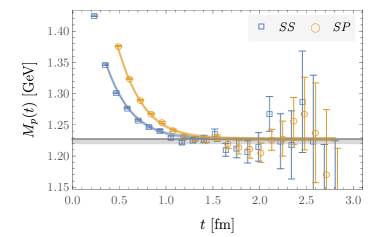
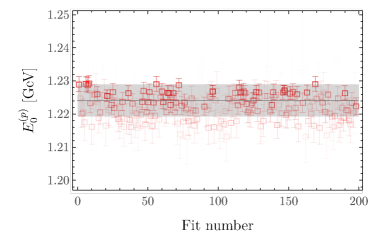
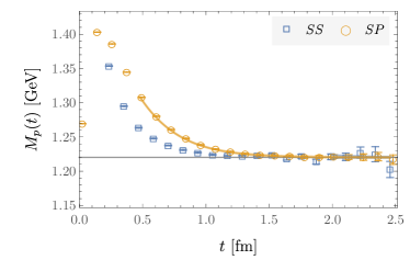
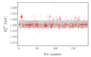
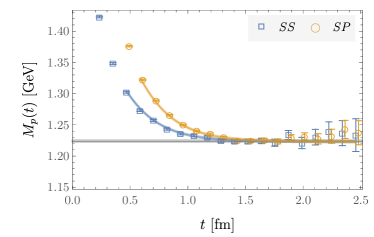
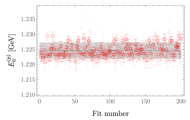
Figure 1: Left column: effective mass functions (Eq. (8)) for the proton correlation function on the E24 (top), E32 (center), and E48 (bottom) ensembles. The orange circles and blue squares show effective masses constructed from SP and SS correlation functions respectively, and the corresponding orange and blue curves display the highest-weight fit contributing to the weighted average of Eq. (6); the light (dark) grey bands show the mass extracted from the weighted average (single highest-weight fit). Right column: masses extracted from each successful fit to the correlators. The opacity of each point is set by the contribution of the fit to the weighted average. The horizontal line and grey band in each figure correspond to the final result for the mass and its total uncertainty.

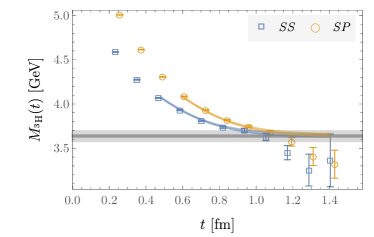
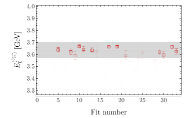
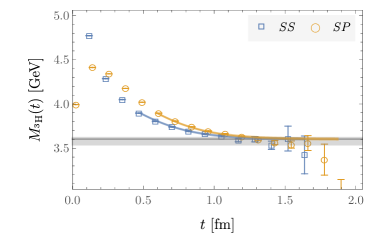
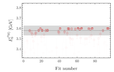
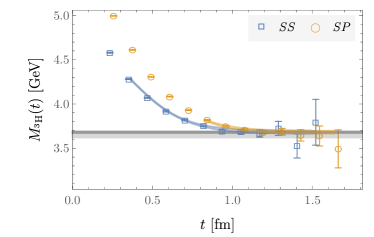
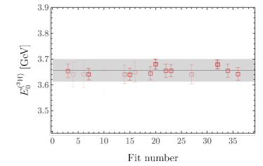
Figure 2: Effective mass functions and fit summaries for the fits of the triton correlation function on the E24 (top), E32 (center), and E48 (bottom) ensembles. All features are as in Fig. 1.

The resulting fitted masses are summarised for each volume in Table 2 and the fits are shown graphically for the proton in Fig. 1 and for the triton in Fig. 2. In each figure, the effective mass functions

$$aM^{\mathcal{SS^{\prime}}}_{h}(t)=\ln\left(\frac{\sum_{s=\pm}C^{\mathcal{SS^{\prime}}}_{h,s}(t)}{\sum_{s=\pm}C^{\mathcal{SS^{\prime}}}_{h,s}(t+a)}\right),$$ (8)

are shown for the SS and SP data along with the functional form of best fits to the correlation functions and the final result for $E_{0}^{(h)}$. The difference between the triton mass and three times the proton mass, $\Delta E_{{}^{3}{\rm H}}=E_{0}^{({}^{3}{\rm H})}-3E_{0}^{(p)}$, is determined from the correlated differences of the fitted energies computed under bootstrap. The results for this quantity are also presented in Table 2.

Ensemble	$aE_{0}^{(p)}$	$aE_{0}^{({}^{3}{\rm H})}$	$a\Delta E_{{}^{3}{\rm H}}$
E24	$0.7258(29)$	$2.157(40)$	$-0.024(32)$
E32	$0.7236(8)$	$2.122(28)$	$-0.054(24)$
E48	$0.7261(16)$	$2.168(26)$	$-0.012(14)$

Table 2: Fit results for the proton and triton ground-state energies, as well as the difference $\Delta E_{{}^{3}{\rm H}}=E_{0}^{({}^{3}{\rm H})}-3E_{0}^{(p)}$, determined in lattice units on each ensemble.

In the limit in which $m_{\pi}L$ is sufficiently large and the pion mass is sufficiently small that the volume dependence of the proton mass is described by $p$-regime chiral perturbation theory ($\chi$PT), that dependence takes the form Ali Khan et al. (2004); Beane (2004)

$$M_{p}(L)-M_{p}^{\infty}=-\frac{3g_{A}^{2}}{8\pi^{2}f_{\pi}^{2}}\mathcal{K}(0,L)-\frac{g_{\Delta N}^{2}}{3\pi^{2}f_{\pi}^{2}}\mathcal{K}(\Delta,L)\,,$$ (9)

where $f_{\pi}$ is the chiral limit pion decay constant and

$$\mathcal{K}(\Delta,L)\equiv\int_{0}^{\infty}d\lambda\beta_{\Delta}\sum_{\vec{n}\neq\vec{0}}\left[(L|\vec{n}|)^{-1}K_{1}\left(L\beta_{\Delta}|\vec{n}|\right)-\beta_{\Delta}K_{0}\left(L\beta_{\Delta}|\vec{n}|\right)\right]\,.$$ (10)

Here, $L$ denotes the spatial extent of the lattice geometry, $K_{n}$ are modified Bessel functions, $\beta_{\Delta}^{2}\equiv\lambda^{2}+2\lambda\Delta+m_{\pi}^{2}$, $\Delta$ denotes the mass splitting between the nucleon and the $\Delta$ baryon, and $g_{\Delta N}$ is the nucleon-$\Delta$ transition axial coupling. The sum in Eq. (10) is over integer triplets excluding $\vec{n}=(0,0,0)$, and for $\Delta=0$ the asymptotic behavior of Eq. (9) is $\sim e^{-m_{\pi}L}/L$. While $m_{\pi}=450$ MeV is not in the regime where chiral perturbation theory shows rapid convergence for baryon properties, it has been found to effectively describe the volume-dependence of baryon masses in this mass regime Beane et al. (2011). With the physical values of $g_{A}=1.26$, $g_{\Delta N}=1.4$, $f_{\pi}=132$ MeV and $\Delta=300$ MeV, Eq. (9) is used to fit to the infinite volume proton mass from the masses determined on the three volumes. This fit, displayed in Figure 3, results in an infinite volume mass of $M_{p}^{\infty}=1.2242(12)$ GeV.

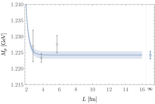
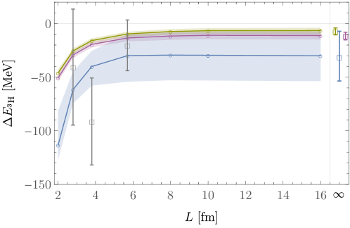
Figure 3: (a) Mass of the proton as a function of the spatial extent of the lattice geometry, along with the fit to this dependence via Eq. (9). (b) The binding energy of the triton as a function of the spatial extent of the lattice geometry. Grey squares correspond to the binding energies determined in the LQCD calculations, while the blue curve shows the finite-volume dependence in pionless EFT fitted to the LQCD data. The blue point at the right indicates the infinite volume extrapolation of the binding energy. For comparison, the binding energies of the $pp$ (purple) and deuteron (green) systems obtained via an analogous FVEFT study are also shown.

Figure 3 also shows the difference between the triton energy and the three-nucleon threshold for each of the three volumes. Unlike for the proton, the form of the volume dependence of the triton energy is not known analytically, however a numerical description can be found by matching to finite-volume effective field theory (FVEFT). The procedure of matching pionless EFT to LQCD results for the binding energies of light nuclei using the stochastic variational method has been demonstrated in Ref. Eliyahu et al. (2020) using LQCD results with $m_{\pi}=806$ MeV. The same procedure as detailed in that work is followed for the data presented here, and further details of the FVEFT approach used here are provided in Appendix A. The infinite volume extrapolation leads to an energy shift $\Delta E_{{}^{3}{\rm H}}^{\infty}=-32(23)$ MeV. The FVEFT formalism is compatible with both scattering states and bound systems and the extracted energy suggests the state is not consistent with three scattering nucleons. This leaves the possibility that it is a compact three-body bound state or either a deuteron–neutron or dineutron-proton scattering state, as the binding energies of the deuteron and dineutron are $7.2(3.2)$ and $11.6(3.6)$ MeV from the FVEFT extrapolation respectively (illustrated in Fig. 9 in Appendix  A; note also that these results are consistent, within 1 standard deviation, with those obtained from this data via Lüscher’s method in Ref. Orginos et al. (2015); Illa et al. (2020)). While the latter cases of 2+1 body systems can not be ruled out, there is a strong preference (80% likelihood, using the most conservative two-body binding energies) that the state is a compact three-body system. In what follows, this is assumed to be the case and the state is referred to as the ‘triton’.

In Fig. 4, the resulting binding energy of the triton is compared to the results of other calculations, including that of Ref. Beane et al. (2013) using the same action but heavier quark masses corresponding to $m_{\pi}=806$ MeV. The extracted binding energy is compatible with those of other calculations at nearby quark masses Yamazaki et al. (2012, 2015), although no effort is made to take into account the differences between the lattice actions or scale-setting schemes that are used. Naive extrapolations of the current result and that from Ref. Beane et al. (2013) that are linear or quadratic in $m_{\pi}$ are consistent with the experimental value for the binding energy of the triton, albeit with large uncertainties. The strong evidence for binding at the other masses shown in the figure, and the assumption of smooth behavior under variation in the pion mass provides additional support for the conclusion that the triton is a compact three-body system at these quark masses.

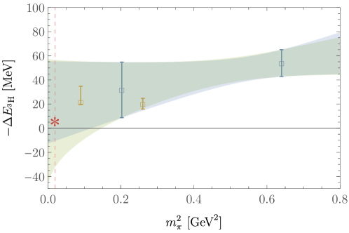
Figure 4: Binding energy of the triton as a function of the pion mass. The current result is shown in blue, along with the result obtained in a previous calculation Beane et al. (2013) using the same action at $m_{\pi}=806$ MeV. The results of Refs. Yamazaki et al. (2012, 2015) are shown in orange. The physical value of the binding is shown as a red star at the physical pion mass, as indicated by the vertical line. Linear and quadratic fits in $m_{\pi}$ to the blue data are shown as the green and blue bands respectively.

IV Gamow-Teller matrix element for tritium $\beta$-decay

To extract the axial charge of the triton, and hence the Gamow-Teller contribution to tritium $\beta$-decay, LQCD calculations of matrix elements of the isovector axial current in the triton and proton are performed using the E32 ensemble. Only a single ensemble is used due to computational cost and for technical simplicity, the flavor-diagonal matrix element $\langle{}^{3}\text{H}|\tilde{A}_{3}^{3}|{}^{3}\text{H}\rangle$ is studied and is related by isospin symmetry to the tritium $\beta$-decay matrix element. The resulting values are matched to FVEFT to determine the relevant low energy constants (LECs), which are then used to predict the infinite-volume matrix element.

To compute the finite-volume matrix elements, the extended propagator technique discussed in detail in Refs. Savage et al. (2017); Shanahan et al. (2017); Tiburzi et al. (2017); Bouchard et al. (2017); Davoudi et al. (2020) is used. This requires extraction of hadronic and nuclear correlation functions at a range of values of an applied constant axial field that couples to up and down quarks separately. Extended quark propagators are defined as

$$S_{\lambda_{f}}^{(f)}(x,y)=S^{(f)}(x,y)+\lambda_{f}\int d^{4}zS^{(f)}(x,z)\gamma_{3}\gamma_{5}S^{(f)}(z,y),$$ (11)

where $S^{(f)}(x,y)$ is a quark propagator of flavor $f\in\{u,d\}$ and $\lambda_{f}$ is the strength of the applied field for the given flavor. These quantities are calculated for five values of the external field strength $\lambda_{u,d}\in\{0,\pm 0.05,\pm 0.1\}$ in lattice units. Two-point correlation functions $C_{h,s}^{(\lambda_{u},\lambda_{d})}(t)$ are constructed from these extended propagators using the same contraction methods as for the zero-field correlation functions discussed in the previous section. For clarity, the smearing labels SS/SP are suppressed in this section. The two-point correlation functions are polynomials in $\lambda_{f}$ of order $n_{f}$, the number of quark propagators of flavor $f$ in the correlation function. With computations at $n_{f}$ different field strength values, the terms in the polynomial can thus be extracted uniquely Tiburzi et al. (2017) and are labelled as $\left.C_{h,s}^{(\lambda_{f},0)}\right|_{{\cal O}(\lambda_{f}^{k})}$ and $\left.C_{h,s}^{(0,\lambda_{f})}\right|_{{\cal O}(\lambda_{f}^{k})}$ for $k\in\{0,\ldots,n_{f}\}$. It is straightforward to show Savage et al. (2017); Tiburzi et al. (2017) through insertions of complete sets of states that an effective isovector axial charge function, which asymptotes to the desired bare axial charge in the corresponding hadronic or nuclear state at large temporal separations, can be defined as

$$g_{A}^{h}(t)=R_{h}(t+a)-R_{h}(t)\underset{t\rightarrow\infty}{\longrightarrow}g_{A}^{h(0)}+{\cal O}(e^{-\delta t}),$$ (12)

where the $(0)$ superscript denotes that the charge is not renormalized, $\delta$ is the energy difference between the ground state and the first excited state with the quantum numbers of the state $h$, and

$$R_{h}(t)=\sum_{s=\pm}\eta_{s}\frac{\left.C_{h,s}^{(\lambda_{u},0)}(t)\right|_{{\cal O}(\lambda_{u})}-\left.C_{h,s}^{(0,\lambda_{d})}(t)\right|_{{{\cal O}(\lambda_{d})}}}{2a\,C_{h,s}^{(0,0)}(t)}$$ (13)

for $\eta_{\pm}=\mp 1$.

The effective charges in Eq. (12) are constructed from sums of ratios of two-point functions whose time dependence is each of the generic exponential form in Eq. (5). The axial charges can therefore be isolated by fits to the time-dependence of the effective charge functions. These fits are performed using an extension of the fit range sampling and excited-state model selection procedure discussed above to background field three-point functions (see Ref. Detmold et al. (2020) for further details). The spectral representations for the $\mathcal{O}(\lambda)$ correlation functions appearing in Eq. (13) can be constructed as

$$\begin{split}\left.C_{h,s}^{(\lambda_{u},0)}(t)\right|_{{\cal O}(\lambda_{u})}-\left.C_{h,s}^{(0,\lambda_{d})}(t)\right|_{{\cal O}(\lambda_{d})}&=a\eta_{s}\sum_{\tau/a=0}^{t/a}\sum_{n,m}{Z_{n}^{(h)}Z_{m}^{(h)\prime\ast}}e^{-E_{n}^{(h)}(t-\tau)}e^{-E_{m}^{(h)}\tau}g_{A}^{h(m,n)(0)},\end{split}$$ (14)

where the prime on the second $Z$-factor is included to denote that, although smearings are suppressed in this section, the overlap factors differ at the source and sink, and the bare (transition) charge $g_{A}^{h(m,n)(0)}$ is defined from the corresponding matrix element as

$$\left<h,n,s\vphantom{\tilde{A}_{3}^{3}h,m,s^{\prime}}\right|\tilde{A}_{3}^{3}\left|h,m,s^{\prime}\vphantom{h,n,s\tilde{A}_{3}^{3}}\right>=\bar{U}_{n,s}\gamma_{3}\gamma_{5}\tau_{3}U_{m,s^{\prime}}g_{A}^{h(m,n)(0)},$$ (15)

where $\left|h,n,s\right>$ denotes states with the quantum numbers of $h$ and $U_{m,s}$ denotes the spinor for state $m$ with spin $s$. This can be used to derive a spectral representation for $g_{A}^{h}(t)$:

$$g_{A}^{h}(t) =\sum_{n}{Z_{n}^{(h)}Z_{n}^{(h)\prime\ast}}g_{A}^{h(n,n)(0)}\left(\frac{(t/a+1)e^{-E_{n}^{(h)}(t+a)}}{\sum_{k}{Z_{k}^{(h)}Z_{k}^{(h)\prime\ast}}e^{-E_{k}^{(h)}(t+a)}}-\frac{(t/a)\,e^{-E_{n}^{(h)}t}}{\sum_{k}{Z_{k}^{(h)}Z_{k}^{(h)\prime\ast}}e^{-E_{k}^{(h)}t}}\right)$$

$$+\mathcal{O}(a),$$ (16)

where the $\mathcal{O}(a)$ contribution is detailed in Ref. Detmold et al. (2020) and depends on excited-state transition matrix elements as well as combinations of overlap factors not determined from fits of two-point functions to Eq. (5). Notably, the $\mathcal{O}(a)$ term is absent for a single-state correlation function model. Multi-state fits have been performed both with and without these $\mathcal{O}(a)$ terms and the AIC is used to determine whether the $\mathcal{O}(a)$ terms should be included in the fit. For both the triton and proton, this AIC test prefers the fit without $\mathcal{O}(a)$ terms for all fit range choices. Combined fits of $\frac{1}{2}\sum_{s=\pm}C_{h,s}(t)$ to Eq. (5) and $g_{A}^{h}(t)$ to Eq. (16) without $\mathcal{O}(a)$ terms using both SP/SS interpolating operator combinations are therefore used to determine $E_{n}^{(h)}$, the product ${Z_{n}^{(h)}Z_{n}^{(h)\prime\ast}}$, and $g_{A}^{h(n,n)}$. For each fitting interval, $\ln(E_{n}^{(h)})$ and $g_{A}^{h(0)}=g_{A}^{h(n,n)(0)}$ are used as nonlinear optimizer parameters with $Z_{n}^{(h)}$ obtained from $C_{h,s}(t)$ using VarPro as above and $g_{A}^{h(n,n)(0)}$ subsequently obtained from $g_{A}^{h}(t)$ using VarPro. Statistical uncertainties on the ground-state matrix elements for each fit are obtained using bootstrap confidence intervals, and a weighted average performed analogously to the two-point function case described above is used to determine the final ground-state matrix element values and statistical plus fitting systematic uncertainties. Results for the ground-state matrix elements $g_{A}^{h{(0)}}$ obtained using this fitting procedure for both one- and three-nucleon systems are shown in Table 3.

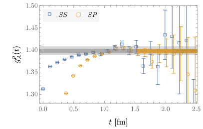
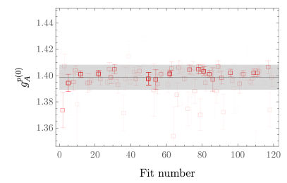
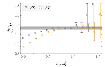
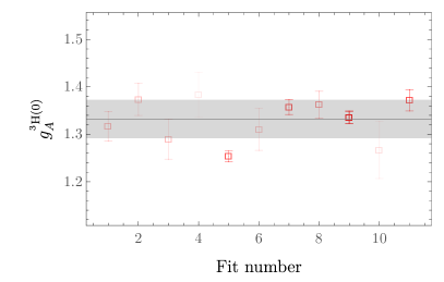
Figure 5: The left panels show the proton and triton bare effective matrix element functions, $g_{A}^{p}(t)$ and $g_{A}^{{}^{3}{\rm H}}(t)$, respectively, calculated on the E32 ensemble. In each figure, the orange (blue) data correspond to the SP (SS) calculations and the corresponding shaded bands illustrate the highest weight fit. The light (dark) shaded gray bands denote the extracted values of the matrix elements arising from the combined analysis (single highest-weight fit). The right panels show the values obtained for all the successful fits to different time ranges, with the opacity determined by the contribution of the fit in the final weighted average. The horizontal line and gray band in the right panels show the final central value and uncertainty.

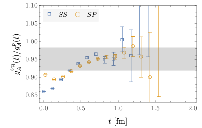
Figure 6: The effective ratio function $g_{A}^{{}^{3}{\rm H}}(t)/g_{A}^{p}(t)$, constructed through Eq. (12), which asymptotes to $g_{A}^{{}^{3}\text{H}}/g_{A}^{p}$ and is independent of axial current renormalization. The orange (blue) data show the SP (SS) correlation functions on the E32 ensemble and the shaded band indicates the extracted value of the matrix element (not a fit to the displayed data).

The quantities $g_{A}^{p}(t)$ and $g_{A}^{{}^{3}{\rm H}}(t)$ constructed on ensemble E32 for both SS and SP source–sink pairs are shown in Fig. 5. Also shown are the values of the bare matrix elements determined from fits to the time-dependence of these functions as discussed above. Table 3 displays the extracted bare couplings $g_{A}^{h(0)}$ as well as renormalized couplings $g_{A}^{h}=Z_{A}g_{A}^{h(0)}$ obtained by multiplying by the appropriate axial current renormalization constant, $Z_{A}=0.8623(01)(71)$ determined in Ref. Yoon et al. (2017). The ratio $g_{A}^{{}^{3}{\rm H}}(t)/g_{A}^{p}(t)$, which at large times asymptotes to the GT reduced matrix element $\langle\mathbf{GT}\rangle=g_{A}^{{}^{3}{\rm H}}/g_{A}^{p}$, and is independent of the renormalization of the axial current, is shown in Fig. 6 along with the value of $\langle\mathbf{GT}\rangle$ that is extracted from the fits to the individual axial couplings.

h	$g_{A}^{h(0)}$	$g_{A}^{h}$	$g_{A}^{h}/g_{A}^{p}$
$p$	$1.399(9)$	$1.230(19)$	–
${}^{3}{\rm H}$	$1.332(40)$	$1.171(39)$	$0.953(30)$

Table 3: Fit results for the bare, $g_{A}^{h(0)}$, and renormalized, $g_{A}^{h}$, axial charges of the proton and triton as well as the corresponding ratio to the axial charge of the proton. The statistical uncertainties and fitting systematic uncertainties are combined in quadrature. The fitting systematic uncertainties account for variation in the choice of fit ranges and multi-state fit models used to obtain $g_{A}^{h(0)}$ and the resulting correlated ratio of ground-state matrix elements $g_{A}^{h}/g_{A}^{p}$ as described in the main text.

The FV three-body matrix element in Table 3 can be used to constrain the leading two-nucleon axial current counterterm of pionless effective field theory in the finite volume. To do so, the approach developed in Ref. W. Detmold and P. E. Shanahan (2021) is followed, whereby EFT wavefunctions, determined variationally and matched to the LQCD spectrum computed in the E32 volume, are used to evaluate the FVEFT matrix elements of the EFT current:

$${\cal A}_{i,a}= \frac{g_{A}}{2}N^{\dagger}\tau_{a}\sigma_{i}N+L_{1,A}\left[\left(N^{T}P_{i}N\right)^{\dagger}\left(N^{T}\bar{P}_{a}N\right)+\text{h.c.}\right]+\ldots,$$ (17)

where $g_{A}$ is the single-nucleon axial coupling, and the projectors

$$P_{i} \equiv\frac{1}{\sqrt{8}}\sigma_{2}\sigma_{i}\tau_{2},\qquad\overline{P}_{a} \equiv\frac{1}{\sqrt{8}}\sigma_{2}\tau_{2}\tau_{a},$$ (18)

form spin-triplet and spin-singlet two-nucleon states, respectively. The two-body couterterm $L_{1,A}$ is regulator-dependent, and in this work a Gaussian regulator scheme is used with a scale $\Lambda$ as discussed in Appendix A.

The ratio of the triton to proton matrix elements in FVEFT is given by

$$\frac{2}{g_{A}}\frac{\langle\Psi_{{}^{3}\text{H}},s=+|{\cal A}_{3,3}|\Psi_{{}^{3}\text{H}},s=+\rangle}{\langle\Psi_{{}^{3}\text{H}},s=+|\Psi_{{}^{3}\text{H}},s=+\rangle}=\left(1+\frac{L_{1,A}}{3g_{A}}h_{{}^{3}\text{H}}(\Lambda,L)\right)\,,$$ (19)

where $|\Psi_{{}^{3}\text{H}},s\rangle$ is the wavefunction for the spin-$s$ ${}^{3}\text{H}$ state and $h_{{}^{3}\text{H}}(\Lambda,L)$ is the spatial expectation value of a regulated form of ${\cal A}_{3,3}$ in the triton spatial wavefunction as detailed in Appendix A. The ratio of LECs $\widetilde{L}_{1,A}\equiv L_{1,A}/g_{A}$ is determined by demanding that Eq. (19) for the E32 volume reproduces the LQCD ratio of axial charges for ${}^{3}\text{H}$ and for the proton computed on that volume. This value of $\widetilde{L}_{1,A}$ is then used to compute the axial current matrix element in variationally-optimised triton wavefunctions for different volumes, including the infinite volume wave function that allows the infinite-volume matrix element to be determined (more details on this procedure are given in Appendix A). While the counterterm $L_{1,A}$ is scheme and scale-dependent, the triton axial charge for any volume is scale-independent. Figure 7 shows the result of this matching procedure and the volume dependence of the ratio of triton to proton axial matrix elements. As expected from the deep binding of this system, the volume effects are small. The resulting infinite-volume GT matrix element is $\langle\mathbf{GT}\rangle_{L=\infty}=g_{A}^{{}^{3}{\rm H}}/g_{A}^{p}=0.938(41)$.

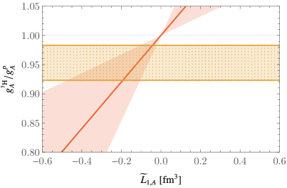
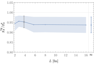
Figure 7: (a) Determination of the LEC ratio $\widetilde{L}_{1,A}$ by matching the matrix element defined in Eq. (19), computed in the optimized FVEFT wavefunction for the E32 volume, to the LQCD result in the E32 volume, which is depicted as the horizontal band. (b) The FVEFT extrapolation of the ratio of triton to proton axial charges to infinite volume.

V Discussion

In order to connect to the physical quark masses, the result for the ratio of triton and proton axial charges described in the last section can be combined with the previous determination of $g_{A}^{{}^{3}{\rm H}}/g_{A}^{p}=0.979(03)(10)$ in Ref. Savage et al. (2017) at the $SU(3)$-symmetric point (where $m_{\pi}=m_{K}=806$ MeV) using the same action and scale setting procedure. Tritium $\beta$-decay has been investigated in $\chi$PT in Ref. Baroni et al. (2018) (see Refs. De-Leon et al. (2016, 2019) for related work in pionless effective field theory) and so the mass dependence of the ratio is in principle known. However, the quark masses in the calculation of Ref. Savage et al. (2017), and potentially in the current work, are beyond the regime of applicability of $\chi$PT. Additionally, for the three-body system of the triton, the effective field theory results are determined numerically rather than analytically. At present, the above discussion, and the paucity of LQCD data, motivates extrapolation of the axial current matrix element ratio with the phenomenological forms of linear and quadratic dependence on the pion mass. The calculated GT matrix elements and both of these extrapolations are shown in Fig. 8; the two fits result in values of 0.90(8) and 0.92(6), respectively. Given the model dependence of the forms used in this extrapolation, the envelope of the extrapolated uncertainties is taken as the extrapolated result, leading to $g_{A}^{{}^{3}{\rm H}}/g_{A}^{p}=0.91$$\begin{subarray}{c}+0.07\\ -0.09\end{subarray}$.

While extrapolated to infinite volume and the physical quark masses, these results are determined at a single lattice spacing and QED and isospin breaking effects are absent and the uncertainties from these systematic effects can as yet only be estimated. Lattice spacing effects are expected to contribute to the matrix elements at ${\cal O}(a\Lambda_{\rm QCD})$, however it is likely that there will be partial cancellations in these effects between the proton and triton axial charges and a full evaluation of this uncertainty will require further calculations. The leading QED effects cancel in the ratio of triton to proton axial charges and isospin breaking effects in $g_{A}^{p}$ have been estimated as $\lesssim 1$ % Jin (1996); Kaiser (2001) and are assumed to be similarly small for the triton. Exponentially-suppressed FV effects due to virtual pions are neglected in the pionless FVEFT formalism that has been used. However, for the volumes and masses used in this work and Ref. Savage et al. (2017), $e^{-m_{\pi}L}\sim 10^{-4}$ so these effects are expected to be negligible.

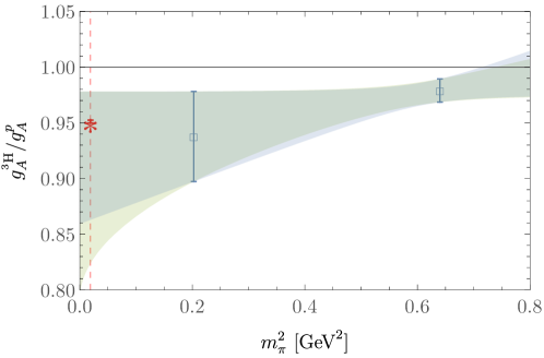
Figure 8: Ratio of the axial charge of tritium to that of the single nucleon as a function of the pion mass. The result from this work and that of Ref. Savage et al. (2017) are shown as the blue points while the physical value Baroni et al. (2016) is shown in red at the physical pion mass (indicated by the vertical line).

The axial charge of the triton is thus extracted from lattice QCD for the first time in this work. The extrapolated coupling ratio is in agreement with the phenomenological value $g_{A}^{{}^{3}{\rm H}}/g_{A}^{p}=0.9511(13)$ Baroni et al. (2016) and thus this calculation demonstrates the QCD origins of nuclear effects in the GT tritium $\beta$-decay matrix element. In the future, the two-body pionless EFT currents that are determined using these methods will also allow for calculations of the GT matrix elements in larger nuclei and a more comprehensive investigation of the QCD origin of the phenomenological quenching of the axial charge.

Appendix A FVEFT

Following Ref. W. Detmold and P. E. Shanahan (2021), the stochastic variational method is used to connect the finite volume axial matrix element to its infinite volume limit in pionless EFT. The pionless EFT Lagrangian relevant to the interaction of few-nucleon systems is

$$\mathcal{L}=\mathcal{L}_{1}+\mathcal{L}_{2}+\mathcal{L}_{3},$$ (20)

where the strong interactions between nucleons arise from

$$\mathcal{L}_{1} =N^{\dagger}\left(iD_{0}+\frac{\mathbf{D}^{2}}{2M_{N}}\right)N+\ldots,$$ (21)

$$\mathcal{L}_{2} =-{C_{S}}\left(N^{T}P_{i}N\right)^{\dagger}\left(N^{T}P_{i}N\right)-{C_{T}}\left(N^{T}\overline{P}_{a}N\right)^{\dagger}\left(N^{T}\overline{P}_{a}N\right)+\ldots,$$ (22)

$$\mathcal{L}_{3} =-\frac{D_{0}}{6}(N^{\dagger}N)^{3}+\ldots,$$ (23)

where $P_{i}$ and $\overline{P}_{a}$ are the projectors defined in Eq. (18), $M_{N}$ is the nucleon mass, and $C_{S}$, $C_{T}$, and $D_{0}$ are the relevant two and three-nucleon low-energy constants (LECs). The two-nucleon couplings can also be expressed in terms of alternative LECs $C_{0,1}$ through the relations

$$C_{T}=C_{0}-3C_{1}\text{ and }C_{S}=C_{0}+C_{1}.$$ (24)

The $n$-particle non-relativistic Hamiltonian corresponding to Eq. (20) is

$$H=-\frac{1}{2M_{N}}\sum_{i}\nabla_{i}^{2}+\sum_{i<j}V_{2}\left({\bf r}_{ij}\right)+\sum_{i<j<k}V_{3}\left({\bf r}_{ij},{\bf r}_{jk}\right),$$ (25)

where the integers $\{i,j,k\}$ label the particle, ${\bf r}_{ij}={\bf r}_{i}-{\bf r}_{j}$ denotes the displacement between particles $i$ and $j$, and the two and three-particle potentials are given by

$$V_{2}\left({\bf r}_{ij}\right)=\left(C_{0}+C_{1}\sigma_{i}\cdot\sigma_{j}\right)g_{\Lambda}\left({\bf r}_{ij},L\right),\hskip 14.22636ptV_{3}\left({\bf r}_{ij},{\bf r}_{jk}\right)=D_{0}\sum_{cyc}g_{\Lambda}\left({\bf r}_{ij},L\right)g_{\Lambda}\left({\bf r}_{jk},L\right).$$ (26)

Here $g_{\Lambda}({\bf r},L)$ includes the Gaussian smearing which is used to regulate the interactions, and periodicity in the finite spatial volume of extent $L$ has been imposed in the regulator:

$$g_{\Lambda}({\bf r},L)=\frac{\Lambda^{3}}{8\pi^{3/2}}\prod_{\alpha=x,y,z}\sum_{q^{(\alpha)}=-\infty}^{\infty}\exp\left(-\Lambda^{2}(r_{\alpha}-Lq^{(\alpha)})^{2}/4\right),$$ (27)

where ${\bf r}=(r_{x},r_{y},r_{z})$.

As described in Refs. Eliyahu et al. (2020); W. Detmold and P. E. Shanahan (2021), the stochastic variational approach proceeds by the optimization of a two or three-body variational wavefunction defined in terms of correlated Gaussian basis components to minimize the expectation value of the Hamiltonian in Eq. (25) and converge to a representation of the ground-state wavefunction. Since rotational symmetry is broken by the lattice geometry, shifted correlated Gaussians are used Eliyahu et al. (2020). Defining a trial wavefunction as a linear combination of such shifted correlated Gaussians, the linear coefficients of the terms are optimized by solving the generalized eigenvalue problem of the variational method; the approach taken to optimization is as detailed in Ref. W. Detmold and P. E. Shanahan (2021). Given wavefunctions optimized in the same volumes as the LQCD calculations, the LECs $C_{S}$, $C_{T}$, and $D_{0}$ of the pionless EFT Lagrangian can be constrained by matching the finite volume energies to the LQCD results, with the allowed range of LECs determined by a fit to the constraints from the three volumes. With the LECs fixed, volume-extrapolated energies are obtained using wavefunctions optimized at infinite volume.

Figure 9 shows the determination of the two-body LECs from the LQCD results for the deuteron and dineutron energy shifts in the three lattice volumes. The couplings are regulator-scale–dependent but the resulting energy shifts are not; calculations with cutoff parameter $\Lambda=\sqrt{2}/r_{0}$ with $r_{0}\in\{0.3,0.4\}$ fm result in indistinguishable results from those with $r_{0}=0.2$ fm which are shown here. The extrapolation to infinite volume using these couplings is shown in Fig. 10. Figure 11 shows the same analysis of the three body system, determining the three-nucleon coupling $D_{0}$ and leading to the infinite-volume extrapolation presented in Fig. 3.

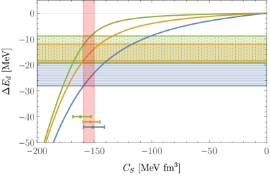
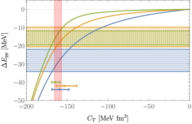
Figure 9: Determination of the EFT two-body couplings, $C_{S,T}$ from the deuteron (left) and $pp$ (right) energies. The horizontal bands correspond to the energy shifts from the LQCD calculations on the E24 (blue), E32 (orange), and E48 (green) ensembles. The curves in each figure show the FVEFT two-body energy shifts for $L\in\{24,32,48\}$ (using the same color scheme) for the EFT cutoff parameter $r_{0}=0.2$ fm W. Detmold and P. E. Shanahan (2021). The LECs are determined by a simultaneous optimization matching the LQCD constraints from all three volumes to the corresponding curves; the results are shown as the red bands. To guide the eye, the intercept ranges of each band with the corresponding curve are shown as the colored bars.

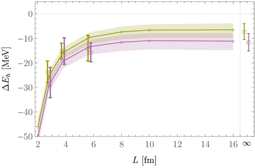
Figure 10: Extrapolation of the deuteron (green) and $pp$ (purple) energies to the infinite volume limit. Data points denote lattice results (from Ref. Orginos et al. (2015)), displaced slightly horizontally for clarity, while the shaded bands and infinite-volume points show the result of the FVEFT extrapolation.

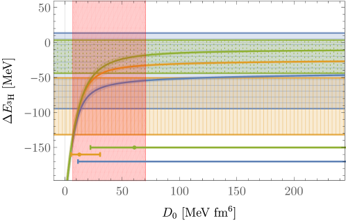
Figure 11: Determination of the EFT three-body couplings $D_{0}$. As in Fig. 9, the horizontal bands correspond to the energy shifts from the LQCD calculations on the E24 (blue), E32 (orange), and E48 (green) ensembles. The curves in each figure show the corresponding FVEFT energy shifts for the EFT cutoff parameter $r_{0}=0.2$ fm. The uncertainties on the curves are propagated from the uncertainties on the two-body LECs.

Using the optimized wavefunctions, matrix elements of the isovector axial-vector current can be computed for the same finite volume as the LQCD calculations to fix the corresponding LECs, and the extrapolation to infinite-volume can then be undertaken in the same manner as that used for the binding energies themselves. The isovector axial-vector current is expressed in pionless EFT as given in Eq. (17) in the main text. In position space, the two-nucleon contribution proportional to $L_{1,A}$ is implemented using the same gaussian regulator as for the potential, specifically

$$L_{1,A}\left[\left(N^{T}({\bf r}_{i})P_{i}N({\bf r}_{i})\right)^{\dagger}\left(N({\bf r}_{j})^{T}\bar{P}_{a}N({\bf r}_{j})\right)+\text{h.c.}\right]g_{\Lambda}({\bf r}_{ij})\,.$$ (28)

The optimised triton wavefunction corresponding to volume of the E32 ensemble is used to compute the finite-volume axial matrix element in Eq. (19). Approximating the triton wavefunction as a tensor product

$$\left|\Psi_{{}^{3}\text{H}},s\right\rangle=\left|\chi_{s}\right\rangle\otimes\left|\psi({\bf r}_{1},{\bf r}_{2},{\bf r}_{3})\right\rangle,$$ (29)

the computation of the matrix elements separates into the spin-isospin and spatial parts. The simplest spin-isospin wavefunction for the spin-up component is given by

$$\left|\chi_{s=+}\right\rangle= \frac{1}{\sqrt{6}}\left[\left|n^{\uparrow}p^{\uparrow}n^{\downarrow}\right>-\left|n^{\downarrow}p^{\uparrow}n^{\uparrow}\right>-\left|p^{\uparrow}n^{\uparrow}n^{\downarrow}\right>\right.\left.+\left|p^{\uparrow}n^{\downarrow}n^{\uparrow}\right>-\left|n^{\uparrow}n^{\downarrow}p^{\uparrow}\right>+\left|n^{\downarrow}n^{\uparrow}p^{\uparrow}\right>\right],$$ (30)

with an analogous expression for the spin-down wavefunction. The spatial part of the matrix element is determined from the variationally-optimized triton wavefunction and is given by

$$h_{{}^{3}\text{H}}(\Lambda,L)=\frac{\int\prod_{k}d^{3}{\bf r}_{k}\sum_{i<j}g_{\Lambda}({\bf r}_{ij})|\psi({\bf r}_{1},{\bf r}_{2},{\bf r}_{3})|^{2}}{\int\prod_{k}d^{3}{\bf r}_{k}|\psi({\bf r}_{1},{\bf r}_{2},{\bf r}_{3})|^{2}}\,,$$ (31)

where $\{i,j,k\}\in\{1,2,3\}$ and $\psi({\bf r}_{1},{\bf r}_{2},{\bf r}_{3})$ is the position-space representation of the spatial wavefunction of the triton.

The LQCD ratio of the triton to proton axial couplings is reproduced by tuning the LEC ratio $\widetilde{L}_{1,A}=L_{1,A}/g_{A}$ in Eq. (19) as shown in Fig. 7. Having fixed this LEC ratio, the infinite-volume matrix element is evaluated using the infinite-volume variational wavefunction, and the volume-dependence is evaluated using wavefunctions optimized at a range of intermediate volumes. Note that just as for the LECs $\{C_{S},C_{T},D_{0}\}$, the LEC ratio $\widetilde{L}_{1,A}$ is determined in the exponential regulator scheme, but the evaluated axial matrix element itself is independent of the choice of regulator.

References

- Wilkinson (1973) D.H. Wilkinson, “Renormalization of the axial-vector coupling constant in nuclear -decay (II),” Nucl. Phys. A 209, 470–484 (1973).
- Brown and Wildenthal (1985) B.A. Brown and B.H. Wildenthal, “Experimental and Theoretical Gamow-Teller Beta-Decay Observables for the sd-Shell Nuclei,” Atom. Data Nucl. Data Tabl. 33, 347–404 (1985).
- Chou et al. (1993) W.-T. Chou, E.K. Warburton, and B.Alex Brown, “Gamow-Teller beta-decay rates for nuclei,” Phys. Rev. C 47, 163–177 (1993).
- Martínez-Pinedo et al. (1996) G. Martínez-Pinedo, A. Poves, E. Caurier, and A.P. Zuker, “Effective in the pf shell,” Phys. Rev. C 53, 2602 (1996), arXiv:nucl-th/9603039 .
- Gysbers et al. (2019) P. Gysbers et al., “Discrepancy between experimental and theoretical -decay rates resolved from first principles,” Nature Phys. 15, 428–431 (2019), arXiv:1903.00047 [nucl-th] .
- Baroni et al. (2016) A. Baroni, L. Girlanda, A. Kievsky, L.E. Marcucci, R. Schiavilla, and M. Viviani, “Tritium -decay in chiral effective field theory,” Phys. Rev. C 94, 024003 (2016), [Erratum: Phys.Rev.C 95, 059902 (2017)], arXiv:1605.01620 [nucl-th] .
- Kraus et al. (2005) Ch. Kraus et al., “Final results from phase II of the Mainz neutrino mass search in tritium beta decay,” Eur. Phys. J. C 40, 447–468 (2005), arXiv:hep-ex/0412056 .
- Aseev et al. (2011) V.N. Aseev et al. (Troitsk), “An upper limit on electron antineutrino mass from Troitsk experiment,” Phys. Rev. D 84, 112003 (2011), arXiv:1108.5034 [hep-ex] .
- Angrik et al. (2005) J. Angrik et al. (KATRIN), KATRIN design report 2004, Tech. Rep. (2005).
- Ashtari Esfahani et al. (2017) Ali Ashtari Esfahani et al. (Project 8), “Determining the neutrino mass with cyclotron radiation emission spectroscopy—Project 8,” J. Phys. G 44, 054004 (2017), arXiv:1703.02037 [physics.ins-det] .
- González-Alonso et al. (2019) Martin González-Alonso, Oscar Naviliat-Cuncic, and Nathal Severijns, “New physics searches in nuclear and neutron decay,” Prog. Part. Nucl. Phys. 104, 165–223 (2019), arXiv:1803.08732 [hep-ph] .
- Crivellin and Hoferichter (2020) Andreas Crivellin and Martin Hoferichter, “Beta decays as sensitive probes of lepton flavor universality,” (2020), arXiv:2002.07184 [hep-ph] .
- Engel and Menéndez (2017) Jonathan Engel and Javier Menéndez, “Status and Future of Nuclear Matrix Elements for Neutrinoless Double-Beta Decay: A Review,” Rept. Prog. Phys. 80, 046301 (2017), arXiv:1610.06548 [nucl-th] .
- Simpson (1987) J. J. Simpson, “Half-life of tritium and the Gamow-Teller transition rate,” Phys. Rev. C35, 752–754 (1987).
- Ademollo and Gatto (1964) M. Ademollo and Raoul Gatto, “Nonrenormalization Theorem for the Strangeness Violating Vector Currents,” Phys. Rev. Lett. 13, 264–265 (1964).
- Fucito et al. (1982) F. Fucito, G. Parisi, and S. Petrarca, “First Evaluation of G(A) / G(V) in lattice QCD in the quenched approximation,” Phys. Lett. B 115, 148–150 (1982).
- Aoki et al. (2020) S. Aoki et al. (Flavour Lattice Averaging Group), “FLAG Review 2019,” Eur. Phys. J. C 80, 113 (2020), arXiv:1902.08191 [hep-lat] .
- Savage et al. (2017) Martin J. Savage, Phiala E. Shanahan, Brian C. Tiburzi, Michael L. Wagman, Frank Winter, Silas R. Beane, Emmanuel Chang, Zohreh Davoudi, William Detmold, and Kostas Orginos, “Proton-Proton Fusion and Tritium Decay from Lattice Quantum Chromodynamics,” Phys. Rev. Lett. 119, 062002 (2017), arXiv:1610.04545 [hep-lat] .
- Orginos et al. (2015) Kostas Orginos, Assumpta Parreño, Martin J. Savage, Silas R. Beane, Emmanuel Chang, and William Detmold, “Two nucleon systems at from lattice QCD,” Phys. Rev. D 92, 114512 (2015), [Erratum:Phys. Rev. D 102, 039903 (2020)], arXiv:1508.07583 [hep-lat] .
- M. Lüscher and P. Weisz (1985) M. Lüscher and P. Weisz, “On-Shell Improved Lattice Gauge Theories,” Commun. Math. Phys. 97, 59 (1985), [Erratum: Commun. Math. Phys.98,433(1985)].
- Sheikholeslami and Wohlert (1985) B. Sheikholeslami and R. Wohlert, “Improved Continuum Limit Lattice Action for QCD with Wilson Fermions,” Nucl. Phys. B259, 572 (1985).
- Illa et al. (2020) Marc Illa et al., “Low-energy Scattering and Effective Interactions of Two Baryons at MeV from Lattice Quantum Chromodynamics,” (2020), arXiv:2009.12357 [hep-lat] .
- Detmold and Orginos (2013) William Detmold and Kostas Orginos, “Nuclear correlation functions in lattice QCD,” Phys. Rev. D87, 114512 (2013), arXiv:1207.1452 [hep-lat] .
- Beane et al. (2013) S. R. Beane, E. Chang, S. D. Cohen, William Detmold, H. W. Lin, T. C. Luu, K. Orginos, A. Parreño, M. J. Savage, and A. Walker-Loud (NPLQCD), “Light Nuclei and Hypernuclei from Quantum Chromodynamics in the Limit of SU(3) Flavor Symmetry,” Phys. Rev. D87, 034506 (2013), arXiv:1206.5219 [hep-lat] .
- Falcioni et al. (1985) M. Falcioni, M.L. Paciello, G. Parisi, and B. Taglienti, “Again on SU(3) glueball mass,” Nucl. Phys. B 251, 624–632 (1985).
- Francis et al. (2019) A. Francis, J.R. Green, P.M. Junnarkar, Ch. Miao, T.D. Rae, and H. Wittig, “Lattice QCD study of the dibaryon using hexaquark and two-baryon interpolators,” Phys. Rev. D 99, 074505 (2019), arXiv:1805.03966 [hep-lat] .
- Hörz et al. (2020) Ben Hörz et al., “Two-nucleon S-wave interactions at the flavor-symmetric point with : a first lattice QCD calculation with the stochastic Laplacian Heaviside method,” (2020), arXiv:2009.11825 [hep-lat] .
- Wagman et al. (2017) Michael L. Wagman, Frank Winter, Emmanuel Chang, Zohreh Davoudi, William Detmold, Kostas Orginos, Martin J. Savage, and Phiala E. Shanahan, “Baryon-Baryon Interactions and Spin-Flavor Symmetry from Lattice Quantum Chromodynamics,” Phys. Rev. D 96, 114510 (2017), arXiv:1706.06550 [hep-lat] .
- Beane et al. (2020) S.R. Beane et al., “Charged multi-hadron systems in lattice QCD+QED,” (2020), arXiv:2003.12130 [hep-lat] .
- Akaike (1974) H. Akaike, “A new look at the statistical model identification,” IEEE Transactions on Automatic Control 19, 716–723 (1974).
- Stein (1956) Charles Stein, “Inadmissibility of the usual estimator for the mean of a multivariate normal distribution,” in Proceedings of the Third Berkeley Symposium on Mathematical Statistics and Probability, Volume 1: Contributions to the Theory of Statistics (University of California Press, Berkeley, Calif., 1956) pp. 197–206.
- Ledoit and Wolf (2004) Olivier Ledoit and Michael Wolf, “A well-conditioned estimator for large-dimensional covariance matrices,” Journal of Multivariate Analysis 88, 365 – 411 (2004).
- Rinaldi et al. (2019) Enrico Rinaldi, Sergey Syritsyn, Michael L. Wagman, Michael I. Buchoff, Chris Schroeder, and Joseph Wasem, “Lattice QCD determination of neutron-antineutron matrix elements with physical quark masses,” Phys. Rev. D99, 074510 (2019), arXiv:1901.07519 [hep-lat] .
- Golub and Pereyra (2003) Gene Golub and Victor Pereyra, “Separable nonlinear least squares: the variable projection method and its applications,” Inverse Problems 19, R1 (2003).
- O’Leary and Rust (2013) Dianne P. O’Leary and Bert W. Rust, “Variable projection for nonlinear least squares problems,” Computational Optimization and Applications 54, 579–593 (2013).
- Ali Khan et al. (2004) A. Ali Khan et al. (QCDSF-UKQCD), “The Nucleon mass in N(f) = 2 lattice QCD: Finite size effects from chiral perturbation theory,” Nucl. Phys. B 689, 175–194 (2004), arXiv:hep-lat/0312030 .
- Beane (2004) Silas R. Beane, “Nucleon masses and magnetic moments in a finite volume,” Phys. Rev. D 70, 034507 (2004), arXiv:hep-lat/0403015 .
- Beane et al. (2011) S.R. Beane, E. Chang, W. Detmold, H.W. Lin, T.C. Luu, K. Orginos, A. Parreño, M.J. Savage, A. Torok, and A. Walker-Loud, “High Statistics Analysis using Anisotropic Clover Lattices: (IV) Volume Dependence of Light Hadron Masses,” Phys. Rev. D 84, 014507 (2011), arXiv:1104.4101 [hep-lat] .
- Eliyahu et al. (2020) Moti Eliyahu, Betzalel Bazak, and Nir Barnea, “Extrapolating Lattice QCD Results using Effective Field Theory,” Phys. Rev. C 102, 044003 (2020), arXiv:1912.07017 [nucl-th] .
- Briceño et al. (2018) Raul A. Briceño, Jozef J. Dudek, and Ross D. Young, “Scattering processes and resonances from lattice QCD,” Rev. Mod. Phys. 90, 025001 (2018), arXiv:1706.06223 [hep-lat] .
- Yamazaki et al. (2012) Takeshi Yamazaki, Ken-ichi Ishikawa, Yoshinobu Kuramashi, and Akira Ukawa, “Helium nuclei, deuteron and dineutron in 2+1 flavor lattice QCD,” Phys. Rev. D 86, 074514 (2012), arXiv:1207.4277 [hep-lat] .
- Yamazaki et al. (2015) Takeshi Yamazaki, Ken-ichi Ishikawa, Yoshinobu Kuramashi, and Akira Ukawa, “Study of quark mass dependence of binding energy for light nuclei in 2+1 flavor lattice QCD,” Phys. Rev. D 92, 014501 (2015), arXiv:1502.04182 [hep-lat] .
- Shanahan et al. (2017) Phiala E. Shanahan, Brian C. Tiburzi, Michael L. Wagman, Frank Winter, Emmanuel Chang, Zohreh Davoudi, William Detmold, Kostas Orginos, and Martin J. Savage, “Isotensor Axial Polarizability and Lattice QCD Input for Nuclear Double- Decay Phenomenology,” Phys. Rev. Lett. 119, 062003 (2017), arXiv:1701.03456 [hep-lat] .
- Tiburzi et al. (2017) Brian C. Tiburzi, Michael L. Wagman, Frank Winter, Emmanuel Chang, Zohreh Davoudi, William Detmold, Kostas Orginos, Martin J. Savage, and Phiala E. Shanahan, “Double- Decay Matrix Elements from Lattice Quantum Chromodynamics,” Phys. Rev. D96, 054505 (2017), arXiv:1702.02929 [hep-lat] .
- Bouchard et al. (2017) Chris Bouchard, Chia Cheng Chang, Thorsten Kurth, Kostas Orginos, and Andre Walker-Loud, “On the Feynman-Hellmann Theorem in Quantum Field Theory and the Calculation of Matrix Elements,” Phys. Rev. D96, 014504 (2017), arXiv:1612.06963 [hep-lat] .
- Davoudi et al. (2020) Zohreh Davoudi, William Detmold, Kostas Orginos, Assumpta Parreño, Martin J. Savage, Phiala Shanahan, and Michael L. Wagman, “Nuclear matrix elements from lattice QCD for electroweak and beyond-Standard-Model processes,” (2020), arXiv:2008.11160 [hep-lat] .
- Detmold et al. (2020) William Detmold, Marc Illa, David J. Murphy, Patrick Oare, Kostas Orginos, Phiala E. Shanahan, Michael L. Wagman, and Frank Winter, “Lattice QCD constraints on the parton distribution functions of ,” (2020), arXiv:2009.05522 [hep-lat] .
- Yoon et al. (2017) Boram Yoon et al., “Isovector charges of the nucleon from 2+1-flavor QCD with clover fermions,” Phys. Rev. D95, 074508 (2017), arXiv:1611.07452 [hep-lat] .
- W. Detmold and P. E. Shanahan (2021) W. Detmold and P. E. Shanahan, “Few-nucleon matrix elements in pionless effective field theory in a finite volume,” (2021).
- Baroni et al. (2018) A. Baroni et al., “Local chiral interactions, the tritium Gamow-Teller matrix element, and the three-nucleon contact term,” Phys. Rev. C98, 044003 (2018), arXiv:1806.10245 [nucl-th] .
- De-Leon et al. (2016) Hilla De-Leon, Lucas Platter, and Doron Gazit, “Tritium -decay in pionless effective field theory,” (2016), arXiv:1611.10004 [nucl-th] .
- De-Leon et al. (2019) Hilla De-Leon, Lucas Platter, and Doron Gazit, “Calculation of an bound-state matrix element in pionless effective field theory,” (2019), arXiv:1902.07677 [nucl-th] .
- Jin (1996) Xue-min Jin, “Isospin breaking in the nucleon isovector axial charge from QCD sum rules,” (1996), arXiv:hep-ph/9602298 .
- Kaiser (2001) Norbert Kaiser, “Isospin breaking in neutron beta decay and SU(3) violation in semileptonic hyperon decays,” Phys. Rev. C 64, 028201 (2001), arXiv:nucl-th/0105043 .
- Edwards and Joó (2005) Robert G. Edwards and Balint Joó (SciDAC, LHPC, UKQCD), “The Chroma software system for lattice QCD,” Lattice field theory. Proceedings, 22nd International Symposium, Lattice 2004, Batavia, USA, June 21-26, 2004, Nucl. Phys. Proc. Suppl. 140, 832 (2005), [,832(2004)], arXiv:hep-lat/0409003 [hep-lat] .
- (56) A. Pochinsky, “Qlua, https://usqcd.lns.mit.edu/qlua.” .
- Clark et al. (2010) M.A. Clark, R. Babich, K. Barros, R.C. Brower, and C. Rebbi, “Solving Lattice QCD systems of equations using mixed precision solvers on GPUs,” Comput. Phys. Commun. 181, 1517–1528 (2010), arXiv:0911.3191 [hep-lat] .
- Babich et al. (2011) R. Babich, M.A. Clark, B. Joo, G. Shi, R.C. Brower, and S. Gottlieb, “Scaling Lattice QCD beyond 100 GPUs,” in SC11 International Conference for High Performance Computing, Networking, Storage and Analysis (2011) arXiv:1109.2935 [hep-lat] .
- Clark et al. (2016) M.A. Clark, Bálint Joó, Alexei Strelchenko, Michael Cheng, Arjun Gambhir, and Richard Brower, “Accelerating Lattice QCD Multigrid on GPUs Using Fine-Grained Parallelization,” (2016), arXiv:1612.07873 [hep-lat] .
- Winter et al. (2014) F. T. Winter, M. A. Clark, R. G. Edwards, and B. Joó, “A framework for lattice qcd calculations on gpus,” in 2014 IEEE 28th International Parallel and Distributed Processing Symposium (2014) pp. 1073–1082.
- Joó et al. (2016) Bálint Joó, Dhiraj D. Kalamkar, Thorsten Kurth, Karthikeyan Vaidyanathan, and Aaron Walden, “Optimizing wilson-dirac operator and linear solvers for intel® knl,” in High Performance Computing, edited by Michela Taufer, Bernd Mohr, and Julian M. Kunkel (Springer International Publishing, Cham, 2016) pp. 415–427.