Tilting the playing field: Dynamical loss functions for machine learning

Abstract

We show that learning can be improved by using loss functions that evolve cyclically during training to emphasize one class at a time. In underparameterized networks, such dynamical loss functions can lead to successful training for networks that fail to find deep minima of the standard cross-entropy loss. In overparameterized networks, dynamical loss functions can lead to better generalization. Improvement arises from the interplay of the changing loss landscape with the dynamics of the system as it evolves to minimize the loss. In particular, as the loss function oscillates, instabilities develop in the form of bifurcation cascades, which we study using the Hessian and Neural Tangent Kernel. Valleys in the landscape widen and deepen, and then narrow and rise as the loss landscape changes during a cycle. As the landscape narrows, the learning rate becomes too large and the network becomes unstable and bounces around the valley. This process ultimately pushes the system into deeper and wider regions of the loss landscape and is characterized by decreasing eigenvalues of the Hessian. This results in better regularized models with improved generalization performance.

I Introduction

In supervised classification tasks, neural networks learn as they descend a loss function that quantifies their performance. Given a task, there are many components of the learning algorithm that may be tuned to improve performance including: hyperparameters such as the initialization scale Glorot and Bengio (2010); Xiao et al. (2018) or learning rate schedule He et al. (2016); the neural network architecture itself Zoph and Le (2016); the types of data augmentation Cubuk et al. (2018); or the optimization algorithm Kingma and Ba (2015). The structure of the loss function also plays an important role in the outcome of learning Choromanska et al. (2015); Soudry and Carmon (2016); Cooper (2018); Verpoort et al. (2020); Ballard et al. (2017); Mannelli et al. (2019); Arous et al. (2019), and it promotes phenomenology reminiscent of physical systems, such as the jamming transition Franz and Parisi (2016); Geiger et al. (2019); Franz et al. (2019a, b); Geiger et al. (2020a, b). A possible strategy to improve learning could be to vary the loss function itself; is it possible to tailor the loss function to the training data and to the network architecture to facilitate learning? The first step along this path is to compare how different loss functions perform under the same conditions, see for example Janocha and Czarnecki (2017); Rosasco et al. (2004); Kornblith et al. (2020). However, the plethora of different types of initializations, optimizers, or hyper-parameter combinations, makes it very difficult to find the best option even for a specified set of tasks. Given that choosing an optimal loss function landscape from the beginning is difficult, one might ask if transforming the landscape continuously during training can lead to a better final result. This takes us to continuation methods, very popular in computational chemistry Stillinger and Weber (1988); Wawak et al. (1998); Wales and Scheraga (1999), which had their machine learning counterpart in curriculum learning Bengio et al. (2009).

Curriculum learning was introduced by Bengio et al. Bengio et al. (2009) as a method to improve training of deep neural networks. They found that learning can be improved when the training examples are not randomly presented but are organized in a meaningful order which illustrates gradually more concepts, and gradually more complex ones. In practice, this “curriculum” can be achieved by weighing the contribution of easier samples (e.g. most common words) to the loss function more at the beginning and increasing the weight of more difficult samples (e.g. less frequent words) at the end of training. In this way one expects to start with a smoothed-out version of the loss landscape that progressively becomes more complex as training progresses. Since its introduction in 2009, curriculum learning has played a crucial role across deep learning Amodei et al. (2016); Graves et al. (2016); Silver et al. (2017). While this approach has been very successful, it often requires additional supervision: for example when labelling images one needs to add a second label for its difficulty. This requirement can render curriculum learning impractical when there is no clear way to evaluate the difficulty of each training example.

These considerations raised by curriculum learning suggest new questions: if continuously changing the landscape facilitates learning, why do it only once? Furthermore, training data is already divided into different classes–is it possible to take advantage of this already-existing label for each training example instead of introducing a new label for difficulty? In physical systems, cyclical landscape variation has proven effective in training memory Keim and Nagel (2011); Keim and Arratia (2014); Pine et al. (2005); Hexner et al. (2020); Sachdeva et al. (2020). In human learning, as well, many educational curricula are developed to expose students to concepts by cycling through them many times rather than learning everything at the same time or learning pieces randomly. Here we extend this approach to neural network training by introducing a dynamical loss function. In short, we introduce a time-dependent weight for each class to the loss function. During training, the weight applied to each class oscillates, shifting within each cycle to emphasize one class after another. We show in this work that this approach improves training and test accuracy in the underparametrized regime, when the neural network was unable to optimize the standard (static) loss function. Even more surprisingly, it improves test accuracy in the overparameterized regime where the landscape is nearly convex and the final training accuracy is always perfect. Finally, we show how changes in the curvature of the landscape during training lead to bifurcation cascades in the loss function that facilitate better learning.

The advantage of using a dynamical loss function can be understood conceptually as follows. The dynamical loss function changes the loss landscape during minimization, so that although the system is always descending in the instantaneous landscape, it can cross loss-barriers in the static version of the loss function in which each class is weighted equally. The process can be viewed as a sort of peristaltic movement in which the valleys of the landscape alternately sink/grow and rise/shrink, pushing the system into deeper and wider valleys. Progress also occurs when the system falls into valleys that narrow too much for a given learning rate, so that the system caroms from one side of the valley to another, propelling the system into different regions of the landscape. This behavior manifests as bifurcation cascades in the loss function that we will explain in terms of eigenvalues of the Hessian and the Neural Tangent Kernel (NTK) Jacot et al. (2018); Lee et al. (2019). Together, this leads networks trained using dynamical loss functions to move towards wider minima – a criterion which has been shown to correlate with generalization performance Zhang et al. (2016).

II Myrtle5 and CIFAR10 phase diagrams

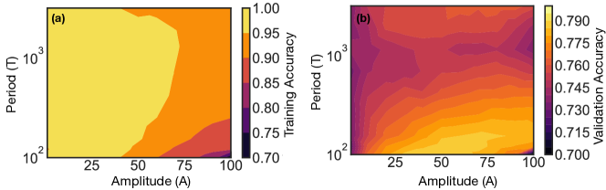
Figure 1: Phase diagrams for the dynamical loss function (1) applied to Myrtle5 Shankar et al. (2020) and CIFAR10. The contour plots represent the training (a) and validation accuracy (b) depending on the amplitude ($A$) and period ($T$) of the oscillations. To create the contour plot we averaged the result of $30$ simulations for each point in a grid in the $(T,A)$ plane. Note that using the standard cross entropy loss function without the oscillations ($\Gamma_{i}=1$, $A=1$ line in both panels) the system already fitted all the training data (training accuracy $\sim 1$) and achieved a $\sim 0.73$ validation accuracy. However, the validation accuracy improved up to $6\%$ thanks to the oscillations for $A\sim 50$ and $T\sim 100$. This neural network is a realistic setup adapted from Shankar et al. (2020). We used $64$ channels, Nesterov optimizer with momentum $=0.9$, minibatch size $512$, a linear learning rate schedule starting at $0$, reaching $0.02$ in the epoch $300$ and decreasing to $0.002$ in the final epoch ($700$). For all $A$ and $T$ the oscillations stopped at epoch $600$ (see the Supplementary Materials for more details).

During learning, we denote the number of minimization steps as $t$. We define a dynamical loss function that is a simple variation of cross entropy and changes during learning:

$$\mathcal{F}=\sum_{j\leq P}\Gamma_{y_{j}}(t)\left(-\log\left(\frac{e^{f_{y_{j}}(x_{j},\mathbf{W})}}{\sum_{i}e^{f_{i}(x_{j},\mathbf{W})}}\right)\right)$$ (1)

Where $\Gamma_{i}$ is a different oscillating factor for each class $i$. We further denote $(x_{j},y_{j})$ to be an element of the the training set of size $P$, $f(x_{j},\mathbf{W})$ is the logit output of the neural network given a training sample $x_{j}$ and the value of the trainable parameters $\mathbf{W}$. Here $f(x_{j},\mathbf{W})\in\mathbb{R}^{C}$ where $C$ is the number of classes. Depending on the values of $\Gamma_{i}$, the topography of the loss function will change, but the loss function will still vanish at the same global minima, which are unaffected by the value of $\Gamma_{i}$. This transformation was motivated by recent work in which the topography of the loss function was changed to improve the tuning of physical flow networks Ruiz-García et al. (2019). Here, we use $\Gamma_{i}$ to emphasize one class relative to the others for a period $T$, and cycle through all the classes in turn so the total duration of a cycle that passes through all classes is $CT$. To simplify the expression, let us define the time within every period $T$ as

$$t_{T}=t\bmod T.$$ (2)

For simplicity we use a function that linearly increases then decreases with amplitude $A$ so that

$$g(t_{T})=\begin{cases}1+mt_{T}&\text{for}\quad 0<t_{T}\leq T/2\\ 2A-mt_{T}-1&\text{for}\quad T/2<t_{T}\leq T\end{cases}$$ (3)

where $A\geq 1$ is the amplitude ($A=1$ corresponds to no oscillations) and $m=2(A-1)/T$. During each period, $\Gamma_{i}$ increases for one class $i$. We cycle through the classes one by one:

$$\hat{\Gamma}_{i}=\begin{cases}g(t_{T})&\text{for}\quad t/T\bmod C=i\\ 1&\text{for}\quad t/T\bmod C\neq i\\ \end{cases}$$ (4)

where $C$ is the number of classes in the dataset. Finally, we normalize these factors,

$$\Gamma_{i}=C\frac{\hat{\Gamma}_{i}}{\sum_{j=1}^{C}\hat{\Gamma}_{j}}.$$ (5)

Figure 4 (a) shows the oscillating factors $\Gamma_{i}$ for the case of a dataset with three classes. Note that due to the normalization, when $\Gamma_{i}$ increases, $\Gamma_{j\neq i}$ decreases.

To test the effect of oscillations on the outcome of training, we use CIFAR10 as a benchmark, without data augmentation. We train the model $30$ times with the same hyperparameter values to average the results over random initializations of $\mathbf{W}$. We use the Myrtle neural network, introduced in Shankar et al. (2020), since it is an efficient convolutional network that achieves good performance with CIFAR10. To obtain enough statistics, we use Myrtle5 with $64$ channels instead of the $1024$ channels used in Ref. Shankar et al. (2020). In all of the experiments we use JAX Bradbury et al. (2018) for training, Neural Tangents for computation of the NTK Novak et al. (2020), and an open source implementation of the Lanczos algorithm for estimating the spectrum of the Hessian Ghorbani et al. (2019a).

In the standard case without oscillations ($A=1$ in Figure 1) this model fits all the training data essentially perfectly (training accuracy $\sim 1$) and achieves a modest $\sim 0.73$ validation accuracy. In figure 1 we vary the amplitude $A$ and period $T$ of oscillations to explore the parameter space of the dynamical loss function. We find a region at $25\lesssim A\lesssim 70$, $T\lesssim 250$ where validation accuracy increases by $\sim 6\%$ to $\sim 0.79$, showing that the dynamical loss function improves generalization significantly.

In addition to the Myrtle5 network, we additionally ran several experiments on a standard Wide Residual Network architecture Zagoruyko and Komodakis (2016) (see Supplementary Information Sec. IV). Over our limited set of experiments, we did not observe a statistically significant improvement to the test accuracy from using an oscillatory loss. We have several hypotheses for why the oscillatory loss was unhelpful in this case: 1) the oscillatory loss may interact poorly with batch normalization, 2) the network is already well-conditioned and so the oscillations may not lead to further improvements to conditioning, and 3) we used a larger batch size than is typical (1024 vs 128) and trained for only 200 epochs; thus, it might be that the model trained in too few steps to take advantage of the oscillations. It is an interesting avenue for future work to disentangle these effects.

III Understanding the effect of the dynamical loss function in a simpler model

III.1 Phase diagrams for the spiral dataset

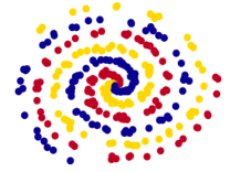
Figure 2: Spiral dataset adapted from Karpathy et al. (2020). Samples are $2$D arrays belonging to three classes, represented by different colors in the image. Each class follows a different spiral arm plus a small noise.

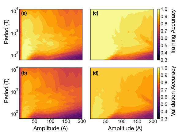
Figure 3: Phase diagrams using the spiral dataset and a neural network with only one hidden layer. We show two examples where the neural network width is $100$ (panels a and b) and $1000$ (panels c and d) respectively. To create the contour plot we averaged the result of $50$ simulations for each point in a grid in the $(T,A)$ plane. In each simulation we used full batch gradient descent for $35000$ steps, a constant learning rate of $1$, and we stopped the oscillations ($\Gamma_{i}=1$) for the last period. The training dataset is shown in Fig. 2 and the validation dataset is analogous to it but with a different distribution of the points along the arms.

To better understand how the oscillations of the dynamical loss function improve generalization, we study a simple but illustrative case. We use synthetic data consisting of points in $2$D that follow a spiral distribution (see Figure 2), with the positions of points belonging to each class following a different arm of the spiral with additional noise (different colors in Fig. 2). In this case we use a neural network with one hidden layer and full batch gradient descent.

Figure 3 shows phase diagrams similar to those in Figure 1, where we vary the amplitude $A$ and period $T$ of oscillation, for two different network widths, which we will call narrow (100 hidden units) and wide (1000 hidden units), respectively. For the narrow network (left side of Fig. 3) with the standard cross-entropy loss function (no oscillations; $A=1$) the model is unable to fit the training data, leading to very poor training and validation accuracies ($\sim 0.65$), suggesting that the standard loss function landscape is complex and the network is unable to find a path to a region of low loss. For the dynamical loss function ($A>1$), on the other hand, there is a region in the phase diagram ($5\lesssim A\lesssim 20$, $T\lesssim 300$), where the training accuracy is nearly perfect and the validation accuracy reaches $\sim 0.9$. Similarly, as we saw in the previous case with Myrtle5 and CIFAR10, when the network is wide enough so that the standard loss landscape is convex (at least in the subspace where training occurs) and the training accuracy is already $\sim 1$ for the standard (static) loss function ($A=1$), there is a regime ($5\lesssim A\lesssim 25$, $T\lesssim 700$) in which the dynamical loss function improves generalization.

III.2 Studying the dynamics of learning with a dynamical loss function in terms of the curvature of the landscape

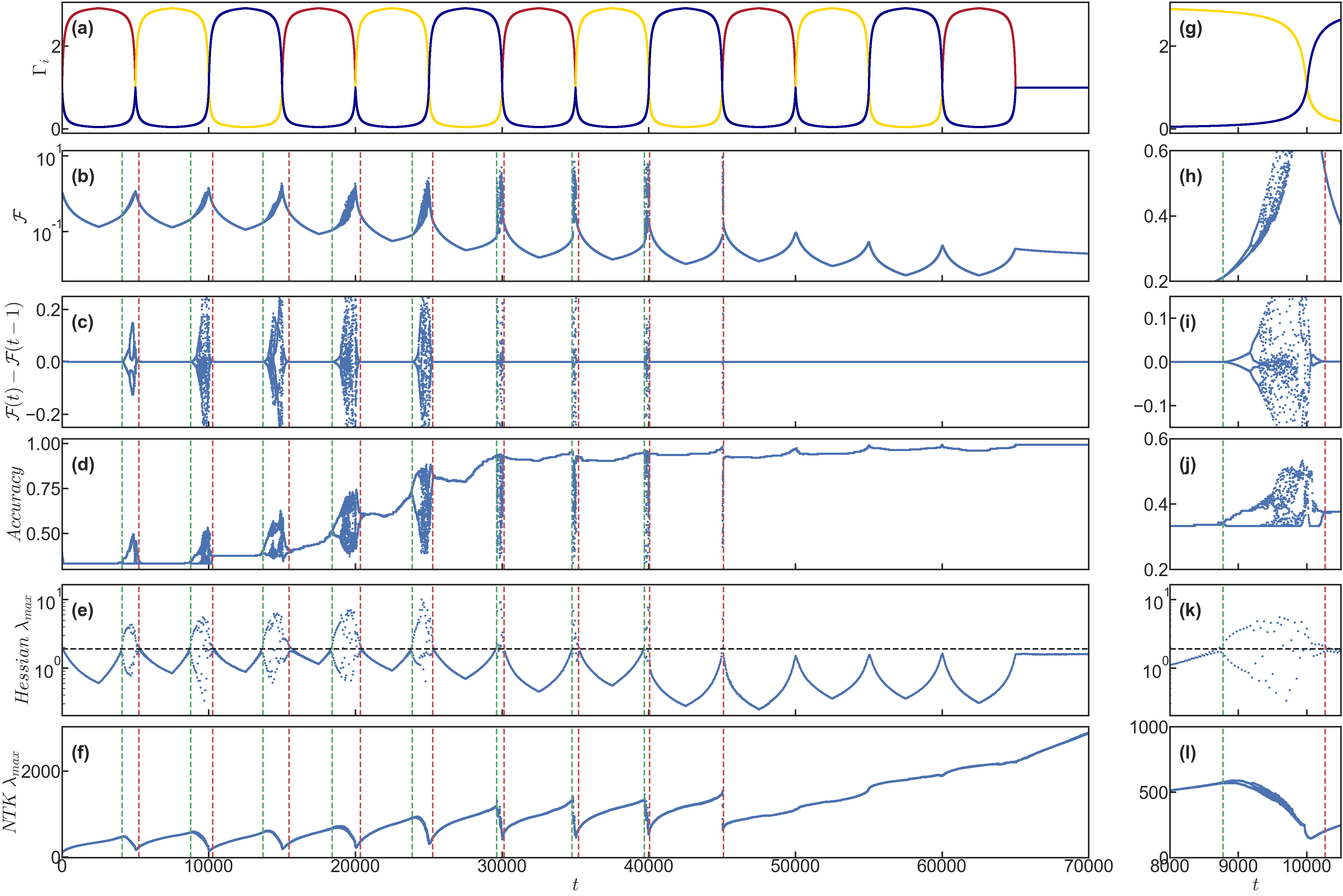
Figure 4: Example of the learning dynamics using a dynamical loss function (1). The width of the hidden layer is $100$. We use $T=5000$ and $A=70$. Panel (a) shows $\Gamma_{i}$ as training progresses, with colors identifying the corresponding classes shown in figure 2. Panel (b) displays the value of the dynamical loss function $\mathcal{F}(t)$. Panel (c) shows $\mathcal{F}(t)-\mathcal{F}(t-1)$ to display the instabilities more clearly. Panel (d) shows the accuracy of the model during training. Panel (e) shows the largest eigenvalue of the Hessian of the loss function computed using the Lanczos algorithm as described in Ghorbani et al. (2019b) (we have used an implementation in Google-JAX Gilmer (2020)) and panel (f) displays the largest eigenvalue of the NTK Jacot et al. (2018). Panels (g-l) correspond to a zoom of panels (a-f) into a region where one bifurcation cascade is present. Vertical green and red dashed lines mark the times at which Hessian $\lambda_{max}(t)-\lambda_{max}(t-1)\sim 0.1$ corresponding to the start and finish of the instabilities. Averaging Hessian $\lambda_{max}$ at these times we get the horizontal dashed line in panel (e), the threshold above which instabilities occur.

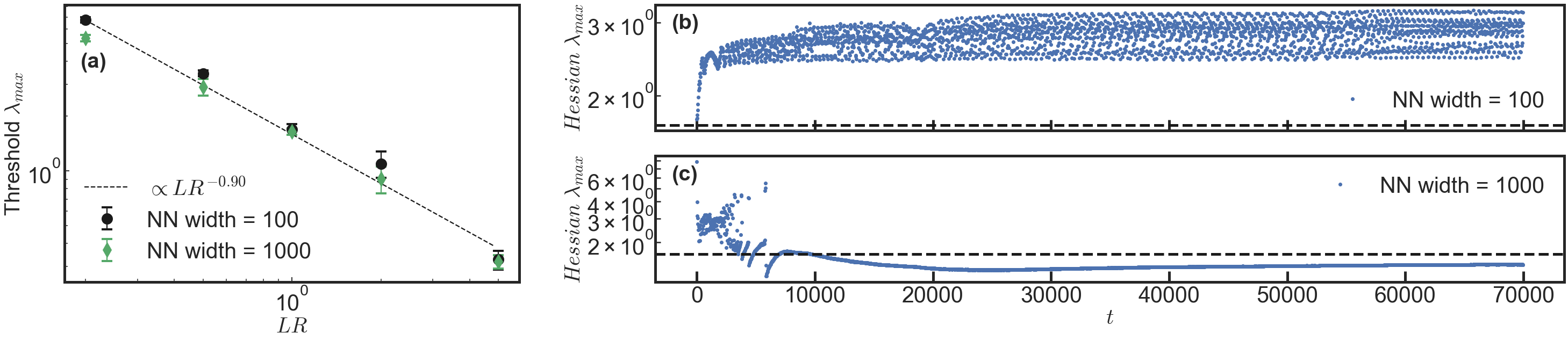
Figure 5: Dependence of the curvature threshold on the learning rate. Panel (a) shows how the threshold of the largest eigenvalue of the Hessian (see Fig. 4) changes as a function of the learning rate for the two NN widths in Fig. 3. Panel (b) and (c) correspond to two simulations without oscillations ($A=1$) and learning rate $1$. The horizontal dashed line marks the threshold (computed in panel (a)). In panel (b) the system does not find a valley that is wide enough, this prevents learning and $\lambda_{max}$ stays above threshold. Panel (c) presents the same case but with a wider network. The system finds a valley that is wide enough to accommodate the learning rate, the model learns the data and after a transitory it stays below the threshold computed in panel (c) using the dynamical loss function.

Let us now take a closer look at the training process to understand how loss function oscillations affect learning. During each period $T$, $\Gamma_{i}>1$ for one class $i$ and $\Gamma_{j\neq i}<1$. In the most extreme case, $A\to\infty$, the network only needs to learn class $i$ during that period. For any initial value of the parameters ($\mathbf{W}$) the model can find a solution (the simplest solution is for the network to output the chosen class regardless of input) without making any uphill moves, and therefore the landscape is convex. However, in the next period the network will have to learn a different class, suggesting that the transition between periods will mark the points at which the topography of the landscape becomes more interesting. (Note that right at the transition all $\Gamma_{i}$ are $1$ and we recover the standard loss function).

Even without the oscillations ($A=1$), the system does not fully reach a minimum of the loss function after training–most of the eigenvalues of the Hessian are very small in modulus (even negative) and only a few of the outliers seem to control learning Sagun et al. (2017, 2016). We will refer not to minima but rather to valleys of the loss function, where we consider the projection of parameter space spanned by large-eigenvalue outliers of the Hessian Gur-Ari et al. (2018).

The behavior of the system as it descends in the dynamical loss function landscape is summarized in Fig. 4, for the spiral dataset for a case with a rather high period of $T=5000$ minimization steps and amplitude of $A=70$, chosen for ease of visualization. Panel (a) shows the values of $\Gamma_{i}$ as learning progresses. Note that due to the normalization (5) these values are bounded between $0$ and $3$ (the number of classes $C$). Panel (b) displays the value of the dynamical loss function at each step: in the first half of each period $T$, the loss function decreases as the system descends in a valley, the change of the loss function in each step is small (panel (c)) and the training accuracy is roughly constant (panel (d)). Panel (e) shows the largest eigenvalue of the Hessian, which provides a measure of the width of the valley; during the first half of the period, the system follows a valley that prioritizes learning samples from the chosen class and the largest eigenvalue decreases (the valley widens) as that class is increasingly emphasized. In this way, the system will move towards a region of parameter space where many (or all) samples belonging to the chosen class are correctly classified.

It follows that during the first half of the oscillation:

• The valley that the system is descending shifts downwards because the network is focusing on learning one class and the contributions to the loss function from the misclassified samples belonging to other classes contribute less and less as learning progresses ($\Gamma_{i}(t)>\Gamma_{i}(t-1)$ and $\Gamma_{j\neq i}(t)<\Gamma_{j\neq i}(t-1)$).

• This valley also widens as other valleys that correctly classify less samples belonging to the chosen class move upwards and shrink (we know about the evolution of the other valleys because it is analogous to the second part of the oscillation, explained below).

In the second half of each oscillation $\Gamma_{i}$ decreases so that the chosen class is now being weighted less and less as time, $t$, progresses. The valley narrows (the largest eigenvalue $\lambda_{max}$ of the Hessian increases; see panel (e)) and rises (the loss function increases even though the system is undergoing gradient descent; see panel (b)).

To summarize, during the second half of each oscillation, we see the following:

• The valley occupied by the system shifts upwards, as the class that the network is focusing on contributes less and less to the loss function and misclassified samples from other classes contribute more ($\Gamma_{i}(t)<\Gamma_{i}(t-1)$ and $\Gamma_{j\neq i}(t)>\Gamma_{j\neq i}(t-1)$).

• The valley also narrows as other valleys that correctly classify samples belonging to other classes grow and sink (as we saw from the first part of the oscillation).

Additionally, during the second part of each period something remarkable happens when Hessian $\lambda_{max}$ crosses a threshold value, marked by the horizontal dashed line in panel (e). At this time (marked by green dashed lines spanning panels (b-f)), a bifurcation instability appears. Panel (c) and (i) show $\mathcal{F}(t)-\mathcal{F}(t-1)$ where the bifurcation instabilities are clearly visible. As $\Gamma_{i}\to 1$ there are additional bifurcation instabilities, forming a cascade.

What is the origin of these bifurcation instabilities? Minimizing the dynamical loss function interweaves two different dynamics: the loss landscape is changing at the same time that the position of the system evolves as it tries to locally minimize the loss function. Thus, both the period $T$ and the learning rate are important. If the learning rate is high enough and the valley is narrow enough, the system is unable to descend the valley and an instability emerges; when other eigenvalues cross this threshold they trigger subsequent bifurcations creating a cascade. A similar phenomenon is described in detail in Lewkowycz et al. (2020) where they discuss early learning dynamics with a large learning rate. At the end of the period $T$ (start of the next period) the loss function begins to emphasize another class. Once the system falls into a valley that is favorable to the new class, the valley widens (Hessian $\lambda_{max}$ decreases) and falls below the learning-rate dependent threshold, so the system no longer bounces and begins to smoothly descend the sinking landscape of that valley. In the specific case depicted in Fig. 4, the system manages after $10$ oscillations to find a valley that is wide enough so that $\lambda_{max}$ never exceeds threshold during subsequent oscillations. To confirm this hypothesis in the next section we study how the curvature threshold at which instabilities emerge depends on the learning rate. See also the Supplementary Materials for simulations where we plot more than one eigenvalue of the Hessian, and for an example of bifurcating dynamics using Myrtle5 to classify CIFAR10.

III.3 Dependence of the threshold on the learning rate.

At each step in the minimization process, the system follows the negative gradient of the loss function, $-\nabla\mathcal{F}$. Taking into account the Taylor series of the loss,

$$\mathcal{F}(\vec{x})\sim\mathcal{F}(\vec{a})+\nabla\mathcal{F}(\vec{a})(\vec{x}-\vec{a})+\frac{1}{2}(\vec{x}-\vec{a})^{T}H\mathcal{F}(\vec{a})(\vec{x}-\vec{a}),$$ (6)

where $H\mathcal{F}(\vec{a})$ is the Hessian matrix evaluated at the point $\vec{a}$, our minimization algorithm may fail when the second order terms are of the same order or larger than the first order terms. This is similar to the upper bound for the learning rate using standard loss functions Le Cun et al. (1991). In this case one step in the direction of $-\nabla\mathcal{F}$ can actually take you to a higher value of the loss, as it occurs in the bifurcation cascades. For a learning rate $\eta$, $(\vec{x}-\vec{a})\propto\eta$, the threshold ($\lambda_{max}^{Th}$) at which the largest eigenvalue of the Hessian makes the first and second order terms in (6) comparable scales as

$$\lambda_{max}^{Th}\propto\eta^{-1},$$ (7)

where we have kept only the term corresponding to the largest eigenvalue of the Hessian in (6). We have also assumed that $-\nabla\mathcal{F}$ is not perpendicular to the eigenvector associated to the largest eigenvalue.

In Fig. 5 (a) we perform simulations equivalent to the one presented in Fig. 4 but with different learning rates. To make the protocol equivalent we rescale the hyperparameters as $T=5000/\eta$ and the total time $70000/\eta$. Panel 5 (a) shows that $\lambda_{max}^{Th}$ does not depend on the network width and it scales as $\sim\eta^{0.9}$, remarkably close to our prediction (7). Furthermore, although these thresholds are computed using the dynamical loss function, they also control learning in the static loss function (the standard cross entropy). Without oscillations, panel (b) depicts how a NN of width $100$ cannot learn with $\eta=1$ because its loss function valleys are too narrow ($\lambda_{max}$ is always above threshold). On the other side, panel (c) shows that after a transitory $\lambda_{max}$ decays below threshold indicating that a wider network produce wider valleys in the loss function what enables learning with higher learning rates. Note that at least in this case, the underparametrized regime prevents learning because the valleys are too narrow for the learning rate. Even if no bad local minima existed, one may be unable to train the network because an unreasonably small learning rate is necessary.

In figure 4 we observed that when the learning rate is too large for the curvature to accommodate, a instability occurs. The values of Hessian $\lambda_{max}$, ${\cal F}$, ${\cal F}(t)-{\cal F}(t-1)$ and training accuracy bifurcate into two branches that the system visits alternatively in each minimization step. This effect can be understood in terms of the gradient and the Hessian of ${\cal F}$: each minimization step is too long for the curvature so that the system bounces between the walls of the valley. However, in the next section we show that the bifurcation in two branches appears naturally when studying the discrete dynamics of the system using the NTK.

III.4 Understanding the bifurcations with the NTK

In addition to the Hessian, the NTK has emerged as a central quantity of interest for understanding the behavior of wide neural networks Jacot et al. (2018); Lee et al. (2019); Yang and Littwin (2021) whose conditioning has been shown to be closely tied to training and generalization Xiao et al. (2020); Dauphin and Schoenholz (2019); Jacot et al. (2019). Even away from the infinite width limit, the NTK can shed light on the dynamics. Figure 4 (f) shows the largest eigenvalue of the NTK. During each of the first 10 oscillations, it increases until the system undergoes a bifurcation instability. It then decreases during the bifurcation cascade. In this section we explain the origin of this phenomenology. We do not develop a rigorous proof but provide the intuition to understand the behavior of the system from the perspective of the NTK.

While the training dynamics in the NTK regime for cross entropy losses have been studied previously Agarwala et al. (2020), here we find that it suffices to consider the case of the Mean Squared Error (MSE) loss. Note that the arguments in this section closely resemble a previous analysis of neural networks at large learning rates Lewkowycz et al. (2020). We write the MSE loss as,

$$\mathcal{L}=\frac{1}{2N}\sum_{i,k}\left(f_{k}(x_{i},\mathbf{W})-y_{i,k}\right)^{2},$$ (8)

where $(x_{i},y_{i,k})$ is the training dataset. Indices $i$ and $k$ are for each sample and class, respectively. $f_{k}(x_{i},\mathbf{W})$ is the output of the neural network (array of dimension $C$) given a training sample $x_{i}$ and the value of the internal parameters of the NN, $\mathbf{W}=\{w_{p}\}$. Using gradient descent, the evolution of parameter $w_{p}$ is

$$\frac{\partial w_{p}}{\partial t} =-\eta\frac{\partial\mathcal{L}}{\partial w_{p}}$$

$$=-\frac{\eta}{N}\sum_{i,k}\frac{\partial f_{k}(x_{i},\mathbf{W})}{\partial w_{p}}\left(f_{k}(x_{i},\mathbf{W})-y_{i,k}\right).$$ (9)

We focus on the evolution of the output of the neural network for an arbitrary sample of the training dataset $x^{\prime}$,

$$\frac{\partial f_{k^{\prime}}(x^{\prime},\mathbf{W})}{\partial t}=\sum_{p}\frac{\partial f_{k^{\prime}}(x^{\prime},\mathbf{W})}{\partial w_{p}}\frac{\partial w_{p}}{\partial t}=$$

$$-\frac{\eta}{N}\sum_{i,k,p}\frac{\partial f_{k^{\prime}}(x^{\prime},\mathbf{W})}{\partial w_{p}}\frac{\partial f_{k}(x_{i},\mathbf{W})}{\partial w_{p}}\left(f_{k}(x_{i},\mathbf{W})-y_{i,k}\right),$$ (10)

and define the NTK as

$$\Theta_{k^{\prime},k^{\prime\prime}}(x^{\prime},x^{\prime\prime})=\sum_{p}\frac{\partial f_{k^{\prime}}(x^{\prime},\mathbf{W})}{\partial w_{p}}\frac{\partial f_{k^{\prime\prime}}(x^{\prime\prime},\mathbf{W})}{\partial w_{p}}.$$ (11)

As an example, in our spiral dataset ($300$ samples and three classes) the NTK can be viewed as a $900$x$900$ matrix. It is useful to consider the difference between the output of the network and the correct label for that sample:

$$g_{k}(x)=\left(f_{k}(x,\mathbf{W})-y_{k}\right).$$ (12)

Combining (10), (11) and (12) one obtains

$$\frac{\partial}{\partial t}g_{k^{\prime}}(x^{\prime})=-\frac{\eta}{N}\sum_{i,k}\Theta_{k^{\prime},k^{\prime\prime}}(x^{\prime},x^{\prime\prime})g_{k}(x_{i}).$$ (13)

In the limit of infinitely small learning rates we can diagonalize the NTK and equation (13) leads to exponential learning of the data, with a rate that is fastest in the directions of the eigenvectors of the NTK associated with the largest eigenvalues. In our case it is more useful to rewrite equation (13) making explicit our discrete dynamics:

$$g^{t+1}_{k^{\prime}}(x^{\prime})=g^{t}_{k^{\prime}}(x^{\prime})-\frac{\eta}{N}\sum_{i,k}\Theta^{t}_{k^{\prime},k^{\prime\prime}}(x^{\prime},x^{\prime\prime})g^{t}_{k}(x_{i}).$$ (14)

Diagonalizing the NTK as $\Theta^{t}_{k^{\prime},k^{\prime\prime}}(x^{\prime},x^{\prime\prime})\tilde{g}_{j}=\lambda_{j}\tilde{g}_{j}$ one finds again a stable learning regime when $0<1-\frac{\eta}{N}\lambda_{j}<1$ (all $\tilde{g}_{j}$ decrease exponentially). When one NTK eigenvalue increases such that $-1<1-\frac{\eta}{N}\lambda_{j}<0$, there is still convergence although $\tilde{g}_{j}$ flips sign with each step. Finally, if one or more eigenvalues cross a threshold such that $1-\frac{\eta}{N}\lambda_{j}<-1$, learning is unstable and the magnitude of $\tilde{g}_{j}$ diverges while the sign flips in each step, creating two branches.

Note that in our case the loss function changes during training, and the NTK (as we have defined it here) cannot account for this change, since it only depends on the data and the parameters $\mathbf{W}$. However, we can interpret the instabilities in Figure 4 in terms of the NTK if we take into account the change of the landscape with an effective learning rate that changes during training. This agrees with our observations: instabilities emerge in the NTK as bifurcations that change sign between one step and the next one (reminiscent of Fig. 4 (c)); after the first bifurcation starts, the largest eigenvalue of the NTK decreases (Fig. 4 (e)) to try to prevent the divergence. Since the values of the NTK largest eigenvalue (Fig. 4 (e)) are not the same every time that a bifurcation starts (as is the case for the largest eigenvalue of the Hessian) we know that the effective learning rate has a non-trivial dependence on the topography of the loss function.

IV Discussion

In this work we have shown that dynamical loss functions can facilitate learning and elucidated the mechanism by which they do so. We have demonstrated that the dynamical loss function can lead to higher training accuracy in the underparametrized region, and can improve the generalization (test or validation accuracy) of overparametrized networks. We have shown this using a realistic model (Myrtle network and CIFAR10) and also using a simple neural network on synthetic data (the spiral dataset). In the latter case we have presented a detailed study of the learning dynamics during gradient descent on the dynamical loss function. In particular, we see that the largest eigenvalue of the Hessian is particularly important in understanding how cycles in the dynamical loss function improve training accuracy by giving rise to bifurcation cascades that allow the system to find wider valleys in the dynamical loss function landscape.

One interesting feature is that the improvement in learning comes in part from using a learning rate that is too fast for the narrowing valley, so that the system bounces instead of descending smoothly within the valley. This feature is somewhat counterintuitive but highly convenient. Our results show that dynamical loss functions introduce new considerations into the trade-off between speed and accuracy of learning.

In the underparametrized case, learning succeeds with the dynamical loss function while it fails with the standard static loss function for the same values of the hyper-parameters. The attention of most practitioners is focused now on the overparametrized limit, where the model has no problem reaching zero training error. However, for complex problems where the overparametrized limit is infeasible, our results suggest that dynamical loss functions can provide a useful path for learning.

Learning each class can be considered a different task, so our approach corresponds to switching tasks in a cyclical fashion. The fact that such switching helps learning may seem to be in contradiction with catastrophic forgetting Goodfellow et al. (2013); Ratcliff (1990); McCloskey and Cohen (1989), where learning new tasks can lead to the forgetting of previous ones. Figure 3 shows that there is an optimum amplitude of the dynamical weighting of the loss function ($A\approx 30$), and that larger values lead to worse performance, in agreement with catastrophic forgetting. Our results show that a strategy that allows learning to proceed on all tasks at all times, but with an oscillating emphasis on one task after another not only avoids catastrophic forgetting but also achieves better results. Our results imply that task-switching schedules should be viewed as a resource for improving learning rather than a liability. Indeed, our results open up a host of interesting questions about how to optimize the choice of static loss function that forms the basis of the dynamical one (e.g. MSE vs. cross entropy) as well as the time-dependence and form of the weighting in the dynamical loss function.

Finally, we note that in the limit $A\to\infty$, the loss function can achieve arbitrarily small values without any uphill moves, starting from any initial weights. The fact that this limit leads to a convex landscape suggests that it could be interesting to carry out a detailed study of the complexity (number of local minima and saddles of different indices) of the landscape as one varies $A$. This could provide additional valuable insight into the learning process for dynamical loss functions. However, it is probably not enough to simply consider minima and saddles–it is clear from our analysis that valleys play an extremely important role and that their width and depth are important. Studying these topographical features of landscapes as $A$ changes should be very enlightening, although likely very challenging.

References

- Glorot and Bengio (2010) X. Glorot and Y. Bengio, in Proceedings of the Thirteenth International Conference on Artificial Intelligence and Statistics, Proceedings of Machine Learning Research, Vol. 9, edited by Y. W. Teh and M. Titterington (JMLR Workshop and Conference Proceedings, Chia Laguna Resort, Sardinia, Italy, 2010) pp. 249–256.
- Xiao et al. (2018) L. Xiao, Y. Bahri, J. Sohl-Dickstein, S. Schoenholz, and J. Pennington, in Proceedings of the 35th International Conference on Machine Learning, Proceedings of Machine Learning Research, Vol. 80, edited by J. Dy and A. Krause (PMLR, Stockholmsmässan, Stockholm Sweden, 2018) pp. 5393–5402.
- He et al. (2016) K. He, X. Zhang, S. Ren, and J. Sun, in 2016 IEEE Conference on Computer Vision and Pattern Recognition (CVPR) (2016) pp. 770–778.
- Zoph and Le (2016) B. Zoph and Q. V. Le, arXiv preprint arXiv:1611.01578 (2016).
- Cubuk et al. (2018) E. D. Cubuk, B. Zoph, D. Mane, V. Vasudevan, and Q. V. Le, arXiv preprint arXiv:1805.09501 (2018).
- Kingma and Ba (2015) D. P. Kingma and J. Ba, CoRR abs/1412.6980 (2015).
- Choromanska et al. (2015) A. Choromanska, M. Henaff, M. Mathieu, G. B. Arous, and Y. LeCun, in Artificial intelligence and statistics (PMLR, 2015) pp. 192–204.
- Soudry and Carmon (2016) D. Soudry and Y. Carmon, arXiv preprint arXiv:1605.08361 (2016).
- Cooper (2018) Y. Cooper, arXiv preprint arXiv:1804.10200 (2018).
- Verpoort et al. (2020) P. C. Verpoort, D. J. Wales, et al., Proceedings of the National Academy of Sciences 117, 21857 (2020).
- Ballard et al. (2017) A. J. Ballard, R. Das, S. Martiniani, D. Mehta, L. Sagun, J. D. Stevenson, and D. J. Wales, Physical Chemistry Chemical Physics 19, 12585 (2017).
- Mannelli et al. (2019) S. S. Mannelli, G. Biroli, C. Cammarota, F. Krzakala, and L. Zdeborová, arXiv preprint arXiv:1907.08226 (2019).
- Arous et al. (2019) G. B. Arous, S. Mei, A. Montanari, and M. Nica, Communications on Pure and Applied Mathematics 72, 2282 (2019).
- Franz and Parisi (2016) S. Franz and G. Parisi, Journal of Physics A: Mathematical and Theoretical 49, 145001 (2016).
- Geiger et al. (2019) M. Geiger, S. Spigler, S. d’Ascoli, L. Sagun, M. Baity-Jesi, G. Biroli, and M. Wyart, Physical Review E 100, 012115 (2019).
- Franz et al. (2019a) S. Franz, S. Hwang, and P. Urbani, Physical review letters 123, 160602 (2019a).
- Franz et al. (2019b) S. Franz, A. Sclocchi, and P. Urbani, Physical review letters 123, 115702 (2019b).
- Geiger et al. (2020a) M. Geiger, A. Jacot, S. Spigler, F. Gabriel, L. Sagun, S. d’Ascoli, G. Biroli, C. Hongler, and M. Wyart, Journal of Statistical Mechanics: Theory and Experiment 2020, 023401 (2020a).
- Geiger et al. (2020b) M. Geiger, L. Petrini, and M. Wyart, arXiv preprint arXiv:2012.15110 (2020b).
- Janocha and Czarnecki (2017) K. Janocha and W. M. Czarnecki, arXiv preprint arXiv:1702.05659 (2017).
- Rosasco et al. (2004) L. Rosasco, E. D. Vito, A. Caponnetto, M. Piana, and A. Verri, Neural Computation 16, 1063 (2004).
- Kornblith et al. (2020) S. Kornblith, H. Lee, T. Chen, and M. Norouzi, arXiv preprint arXiv:2010.16402 (2020).
- Stillinger and Weber (1988) F. Stillinger and T. Weber, Journal of statistical physics 52, 1429 (1988).
- Wawak et al. (1998) R. J. Wawak, J. Pillardy, A. Liwo, K. D. Gibson, and H. A. Scheraga, The Journal of Physical Chemistry A 102, 2904 (1998).
- Wales and Scheraga (1999) D. J. Wales and H. A. Scheraga, Science 285, 1368 (1999).
- Bengio et al. (2009) Y. Bengio, J. Louradour, R. Collobert, and J. Weston, in Proceedings of the 26th annual international conference on machine learning (2009) pp. 41–48.
- Amodei et al. (2016) D. Amodei, S. Ananthanarayanan, R. Anubhai, J. Bai, E. Battenberg, C. Case, J. Casper, B. Catanzaro, Q. Cheng, G. Chen, J. Chen, J. Chen, Z. Chen, M. Chrzanowski, A. Coates, G. Diamos, K. Ding, N. Du, E. Elsen, J. Engel, W. Fang, L. Fan, C. Fougner, L. Gao, C. Gong, A. Hannun, T. Han, L. Johannes, B. Jiang, C. Ju, B. Jun, P. LeGresley, L. Lin, J. Liu, Y. Liu, W. Li, X. Li, D. Ma, S. Narang, A. Ng, S. Ozair, Y. Peng, R. Prenger, S. Qian, Z. Quan, J. Raiman, V. Rao, S. Satheesh, D. Seetapun, S. Sengupta, K. Srinet, A. Sriram, H. Tang, L. Tang, C. Wang, J. Wang, K. Wang, Y. Wang, Z. Wang, Z. Wang, S. Wu, L. Wei, B. Xiao, W. Xie, Y. Xie, D. Yogatama, B. Yuan, J. Zhan, and Z. Zhu, in Proceedings of The 33rd International Conference on Machine Learning, Proceedings of Machine Learning Research, Vol. 48, edited by M. F. Balcan and K. Q. Weinberger (PMLR, New York, New York, USA, 2016) pp. 173–182.
- Graves et al. (2016) A. Graves, G. Wayne, M. Reynolds, T. Harley, I. Danihelka, A. Grabska-Barwińska, S. G. Colmenarejo, E. Grefenstette, T. Ramalho, J. Agapiou, et al., Nature 538, 471 (2016).
- Silver et al. (2017) D. Silver, J. Schrittwieser, K. Simonyan, I. Antonoglou, A. Huang, A. Guez, T. Hubert, L. Baker, M. Lai, A. Bolton, et al., nature 550, 354 (2017).
- Keim and Nagel (2011) N. C. Keim and S. R. Nagel, Physical review letters 107, 010603 (2011).
- Keim and Arratia (2014) N. C. Keim and P. E. Arratia, Physical review letters 112, 028302 (2014).
- Pine et al. (2005) D. J. Pine, J. P. Gollub, J. F. Brady, and A. M. Leshansky, Nature 438, 997 (2005).
- Hexner et al. (2020) D. Hexner, A. J. Liu, and S. R. Nagel, Proceedings of the National Academy of Sciences 117, 31690 (2020).
- Sachdeva et al. (2020) V. Sachdeva, K. Husain, J. Sheng, S. Wang, and A. Murugan, Proceedings of the National Academy of Sciences 117, 12693 (2020).
- Jacot et al. (2018) A. Jacot, F. Gabriel, and C. Hongler, in Advances in neural information processing systems (2018) pp. 8571–8580.
- Lee et al. (2019) J. Lee, L. Xiao, S. Schoenholz, Y. Bahri, R. Novak, J. Sohl-Dickstein, and J. Pennington, in Advances in neural information processing systems (2019) pp. 8572–8583.
- Zhang et al. (2016) C. Zhang, S. Bengio, M. Hardt, B. Recht, and O. Vinyals, arXiv preprint arXiv:1611.03530 (2016).
- Shankar et al. (2020) V. Shankar, A. Fang, W. Guo, S. Fridovich-Keil, J. Ragan-Kelley, L. Schmidt, and B. Recht, in International Conference on Machine Learning (PMLR, 2020) pp. 8614–8623.
- Ruiz-García et al. (2019) M. Ruiz-García, A. J. Liu, and E. Katifori, Physical Review E 100, 052608 (2019).
- Bradbury et al. (2018) J. Bradbury, R. Frostig, P. Hawkins, M. J. Johnson, C. Leary, D. Maclaurin, G. Necula, A. Paszke, J. VanderPlas, S. Wanderman-Milne, and Q. Zhang, “JAX: composable transformations of Python+NumPy programs,” (2018).
- Novak et al. (2020) R. Novak, L. Xiao, J. Hron, J. Lee, A. A. Alemi, J. Sohl-Dickstein, and S. S. Schoenholz, in International Conference on Learning Representations (2020).
- Ghorbani et al. (2019a) B. Ghorbani, S. Krishnan, and Y. Xiao, CoRR abs/1901.10159 (2019a), 1901.10159 .
- Zagoruyko and Komodakis (2016) S. Zagoruyko and N. Komodakis, CoRR abs/1605.07146 (2016), arXiv:1605.07146 .
- Karpathy et al. (2020) A. Karpathy et al., Course notes hosted on GitHub. Retrieved from: http://cs231n. github. io (2020).
- Ghorbani et al. (2019b) B. Ghorbani, S. Krishnan, and Y. Xiao, arXiv preprint arXiv:1901.10159 (2019b).
- Gilmer (2020) J. Gilmer, “Large scale spectral density estimation for deep neural networks,” https://github.com/google/spectral-density (2020).
- Sagun et al. (2017) L. Sagun, U. Evci, V. U. Guney, Y. Dauphin, and L. Bottou, arXiv preprint arXiv:1706.04454 (2017).
- Sagun et al. (2016) L. Sagun, L. Bottou, and Y. LeCun, arXiv preprint arXiv:1611.07476 (2016).
- Gur-Ari et al. (2018) G. Gur-Ari, D. A. Roberts, and E. Dyer, arXiv preprint arXiv:1812.04754 (2018).
- Lewkowycz et al. (2020) A. Lewkowycz, Y. Bahri, E. Dyer, J. Sohl-Dickstein, and G. Gur-Ari, arXiv preprint arXiv:2003.02218 (2020).
- Le Cun et al. (1991) Y. Le Cun, I. Kanter, and S. A. Solla, Physical Review Letters 66, 2396 (1991).
- Yang and Littwin (2021) G. Yang and E. Littwin, “Tensor programs iib: Architectural universality of neural tangent kernel training dynamics,” (2021), arXiv:2105.03703 [cs.LG] .
- Xiao et al. (2020) L. Xiao, J. Pennington, and S. Schoenholz, in Proceedings of the 37th International Conference on Machine Learning, Proceedings of Machine Learning Research, Vol. 119, edited by H. D. III and A. Singh (PMLR, 2020) pp. 10462–10472.
- Dauphin and Schoenholz (2019) Y. N. Dauphin and S. Schoenholz, in Advances in Neural Information Processing Systems, Vol. 32, edited by H. Wallach, H. Larochelle, A. Beygelzimer, F. d’ Alché-Buc, E. Fox, and R. Garnett (Curran Associates, Inc., 2019).
- Jacot et al. (2019) A. Jacot, F. Gabriel, and C. Hongler, CoRR abs/1907.05715 (2019), arXiv:1907.05715 .
- Agarwala et al. (2020) A. Agarwala, J. Pennington, Y. N. Dauphin, and S. S. Schoenholz, CoRR abs/2010.07344 (2020), arXiv:2010.07344 .
- Goodfellow et al. (2013) I. J. Goodfellow, M. Mirza, D. Xiao, A. Courville, and Y. Bengio, arXiv preprint arXiv:1312.6211 (2013).
- Ratcliff (1990) R. Ratcliff, Psychological review 97, 285 (1990).
- McCloskey and Cohen (1989) M. McCloskey and N. J. Cohen, in Psychology of learning and motivation, Vol. 24 (Elsevier, 1989) pp. 109–165.
- Towns et al. (2014) J. Towns, T. Cockerill, M. Dahan, I. Foster, K. Gaither, A. Grimshaw, V. Hazlewood, S. Lathrop, D. Lifka, G. D. Peterson, et al., Computing in science & engineering 16, 62 (2014).