Abstract

The count-min sketch (CMS) is a randomized data structure that provides estimates of tokens’ frequencies in a large data stream using a compressed representation of the data by random hashing. In this paper, we rely on a recent Bayesian nonparametric (BNP) view on the CMS to develop a novel learning-augmented CMS under power-law data streams. We assume that tokens in the stream are drawn from an unknown discrete distribution, which is endowed with a normalized inverse Gaussian process (NIGP) prior. Then, using distributional properties of the NIGP, we compute the posterior distribution of a token’s frequency in the stream, given the hashed data, and in turn corresponding BNP estimates. Applications to synthetic and real data show that our approach achieves a remarkable performance in the estimation of low-frequency tokens. This is known to be a desirable feature in the context of natural language processing, where it is indeed common in the context of the power-law behaviour of the data.

1 Introduction

When processing large data streams of data, it is critical to represent the data in compact structures that allow to efficiently extract statistical information. Sketching algorithms, or simply sketches, are randomized data structures that can be easily updated and queried to perform a time and memory efficient estimation of statistics of large data streams of tokens. Sketches have found numerous applications in, e.g., machine learning (Aggarwal and Yu,, 2010), security analysis (Dwork et al.,, 2010), natural language processing (Goyal et al.,, 2009), computational biology (Zhang et al.,, 2014), social networks (Song et al.,, 2009) and games (Harrison,, 2010). Of particular interest is the problem of estimating the unknown frequency of a token in a stream, which is typically referred to as a “point query". A notable approach to address point queries is the count-min sketch (CMS) (Cormode and Muthukrishnan, 2005b, ; Cormode and Muthukrishnan, 2005a, ), which uses random hashing to obtain a compressed, or approximated, representation of tokens’ frequencies in the stream. The CMS achieves the goal of using a memory efficient representation of the data stream, while having provable theoretical guarantees on the estimated point query via hashed frequencies. In the recent years, there has been an increasing interest in improving the performance of the CMS by means of learning models that allow to better exploit properties of the data. (Cai et al.,, 2018; Aamand et al.,, 2019; Hsu et al.,, 2019). In this paper, we focus on the learning-augmented CMS of (Cai et al.,, 2018), which relies on Bayesian nonparametric (BNP) modeling of a data stream of tokens.

The learning-augmented CMS of Cai et al., (2018) assumes that tokens in a stream are modeled as random samples from an unknown discrete distribution, which is endowed with a Dirichlet process (DP) prior (Ferguson,, 1973). Under this BNP framework, the predictive distribution induced by the DP provides a natural generative scheme for tokens. That is, predictive distributions, combined with both a restriction property and a finite-dimensional projective property of the DP, lead to the posterior distribution of a point query, given the hashed frequencies. This is referred to as the CMS-DP. Interestingly, the posterior mode recovers the CMS estimate of Cormode and Muthukrishnan, 2005a , while other CMS-DP estimates, e.g. posterior mean and median, may be viewed as CMS estimates with shrinkage. The CMS-DP improves over the CMS on several aspects: i) it incorporates a priori knowledge on the data into the estimates; ii) it assumes an unknown and unbounded number of distinct tokens, which is typically expected in large datasets; iii) it allows to model, via the posterior distribution induced by a point query, the uncertainty induced by the process of random hashing.

We extend the BNP approach of Cai et al., (2018) to develop a novel learning-augmented CMS under power-law data streams. Power-law distributions occur in many situations of scientific interest, and have significant consequences for the understanding of natural and man-made phenomena (Clauset et al.,, 2009). Here, we assume that tokens in the stream are modeled as random samples from an unknown discrete distribution, which is endowed with a normalized inverse Gaussian process (NIGP) prior (Prünster,, 2002; Lijoi et al.,, 2005). The NIGP comes as a “forced" choice since it is the sole discrete nonparametric prior that combines: i) a power-law tail behaviour, in contrast with the exponential tail behaviour of the DP; ii) both a restriction property and a finite-dimensional projective property analogous to those of the DP, which are critical to compute and work with the posterior distribution of a point query given the hashed frequencies. While this prior choice limits the flexibility of tuning the prior to the power-law degree of the data, the NIGP is arguably still a sensible choice of practical interest. Under the NIGP prior, we compute the posterior distribution of a point query, given the stored hashed frequencies, and in turn corresponding BNP estimates. Applications to synthetic and real data show that our approach outperforms the CMS and the CMS-DP in the estimation of low-frequency tokens. This is known to be a desirable feature in the context of natural language processing (Goyal et al.,, 2012, 2009; Pitel and Fouquier,, 2015), where it is indeed common the power-law behaviour of the data stream.

The paper is structured as follows. In Section 2 we review the BNP approach to CMS of Cai et al., (2018), and in Section 3 we extend this approach to develop a novel learning-augmented CMS under power-law data streams. Section 4 contains numerical experiments, whereas Section 5 concludes with final remarks and future works.

2 A BNP approach to CMS

To introduce the BNP approach of Cai et al., (2018), let $X_{1:m}=(X_{1},\ldots,X_{m})$ be a large data stream of tokens taking values in a (possibly infinite) measurable space of symbols $\mathcal{V}$. The stream $X_{1:m}$ is available for inferential purposes only through its compressed representation obtained by means of random hashing. Specifically, let $J$ and $N$ be positive integers such that $[J]=\{1,\ldots,J\}$ and $[N]=\{1,\ldots,N\}$, and let $h_{1},\ldots,h_{N}$, with $h_{n}:\mathcal{V}\rightarrow[J]$, be a collection of hash functions drawn uniformly at random from a pairwise independent hash family $\mathcal{H}$. For mathematical convenience it is assumed that $\mathcal{H}$ is a perfectly random hash family, that is for $h_{n}$ drawn uniformly at random from $\mathcal{H}$ the random variables $(h_{n}(x))_{x\in\mathcal{V}}$ are i.i.d. as a Uniform distribution over $[J]$. In practice, as discussed in Cai et al., (2018), real-world hash functions yield only small perturbations from perfect hash functions. Hashing $X_{1:m}$ through $h_{1},\ldots,h_{N}$ creates $N$ vectors of $J$ buckets $\{\mathbf{C}_{n}\}_{n\in[N]}$, where $\mathbf{C}_{n}=(C_{n,1},\ldots,C_{n,J})$ with $C_{n,j}$ obtained by aggregating the frequencies for all $x$ such that $h_{n}(x)=j$. Every $C_{n,j}$ is initialized at zero, and whenever a new token $X_{i}$ is observed we set $C_{n,h_{n}(X_{i})}\leftarrow 1+C_{n,h_{n}(X_{i})}$ for every $n\in[N]$. Under this setting, the goal consists in estimating the frequency $f_{v}$ of a token of type $v\in\mathcal{V}$ in $X_{1:m}$, i.e. the point query $f_{v}=\sum_{1\leq i\leq m}\bm{1}_{X_{i}}(v)$. In particular, the CMS of Cormode and Muthukrishnan, 2005a estimates $f_{v}$ with

$$\hat{f}_{v}^{\text{{(CMS)}}}=\min_{n\in[N]}\{C_{n,h_{n}(v)}\}_{n\in[N]}.$$ (1)

We refer to Appendix A for a detailed account on the CMS and a theoretical (probabilistic) guarantee for the estimator (1).

Differently from the CMS of Cormode and Muthukrishnan, 2005a , the CMS-DP of Cai et al., (2018) estimates $f_{v}$ by relying on the following modeling assumptions on the data stream $X_{1:m}$: i) symbols $v_{j}$’s in $\mathcal{V}$ are distributed as an unknown probability measure $P(\cdot)=\sum_{j\geq 1}p_{j}\delta_{v_{j}}(\cdot)$ on $\mathcal{V}$; ii) $P$ is distributed as a DP prior (Ferguson,, 1973) with diffuse probability (base) measure $\nu$ on $\mathcal{V}$ and mass parameter $\alpha>0$. Then, tokens $X_{i}$’s are modeled as random samples from a DP, i.e.,

$$X_{1:m}\mid P \,\stackrel{{\scriptstyle\mbox{{iid}}}}{{\sim}}\,P$$

$$P \,\sim\,\mathrm{DP}(\alpha,\nu)$$ (2)

for $m\geq 1$. Under (2), a point query induces the posterior distribution of $f_{v}$, given $\{C_{n,h_{n}(v)}\}_{n\in[N]}$, for $v\in\mathcal{V}$. CMS-DP estimates of $f_{v}$ are obtained as functionals of the posterior distribution, e.g. mode, mean, median. The computation of the posterior distribution of $f_{v}$ relies on the predictive distribution of the DP prior, namely the conditional distribution of an additional token given the stream of tokens. This is combined with two critical properties of the DP: P1) the restriction property which, due to the perfectly random $\mathcal{H}$, implies that the prior governing the tokens hashed in each of the $J$ buckets is a DP prior with mass parameter $\alpha/J$; P2) the finite-dimensional projective property which, due to the perfectly random $\mathcal{H}$, implies that the prior governing the multinomial hashed frequencies $\mathbf{C}_{n}$ is a $J$-dimensional symmetric Dirichlet distribution with parameter $\alpha/J$.

Now, we outline the BNP approach of Cai et al., (2018) based properties P1) and P2). Because of the discreteness of $P\sim\mathrm{DP}(\alpha,\nu)$, a random sample $X_{1:m}$ from $P$ induces a random partition of $\{1,\ldots,m\}$ into subsets labelled by distinct symbols in $\mathcal{V}$. See Appendix C. The predictive distribution of the DP provides the conditional distribution, given $X_{1:m}$, over which partition subset a new token $X_{m+1}$ will join; the size of that subset is precisely the frequency $f_{v}$ we seek to estimate. However, since we have only access to the hashed frequencies, the object of interest is the distribution $p_{f_{v}}(m,\alpha)$ of $f_{v}$. This distribution follows by marginalizing out the sampling information $X_{1:,m}$, with respect to the DP prior, from the conditional distribution of $f_{v}$ given $X_{1,m}$. According to property P1), for a single $h_{n}$ the distribution $p_{f_{v}}(\cdot;c_{n,h_{n}(v)},\alpha/J)$ coincides with the posterior distribution of $f_{v}$, given $C_{n,h_{n}(v)}=c_{n,h_{n}(v)}$; the posterior distribution of $f_{v}$ given $\{C_{n,h_{n}(v)}\}_{n\in[N]}$ follows by the independence assumption on $\mathcal{H}$ and Bayes theorem. To conclude, it remains to estimate the prior’s parameter $\alpha>0$ based on the hashed frequencies. According to property P2), and by the independence assumption on $\mathcal{H}$, the $N$ vectors $\{\mathbf{C}_{n}\}_{n\in[N]}$ are i.i.d. as a Dirichlet-Multinomial distribution with symmetric parameter $\alpha/J$. This fact provides an explicit expression for the likelihood function of the hashed frequencies, and thus to a Bayesian estimation of $\alpha$.

3 A BNP approach to CMS under power-law data streams

We extend the BNP approach of Cai et al., (2018) to develop a novel learning-augmented CMS under power-law data streams. In this respect, it is natural to assume that tokens in a stream $X_{1:m}$ are modeled as random samples from an unknown discrete distribution $P$, and then to endow $P$ with prior distribution $\mathcal{Q}$ with power-law tail behaviour. Critical constraints in the choice of $\mathcal{Q}$ arises directly from the approach of Cai et al., (2018). In particular, the prior $\mathcal{Q}$ must feature both a restriction property and a finite-dimensional projective property analogous to those of the DP prior. This is required to compute and work with the posterior distribution of a point query, given the hashed data stream $X_{1:m}$. To the best of our knowledge, the NIGP prior (Prünster,, 2002; Lijoi et al.,, 2005) is the sole discrete nonparametric prior with power-law tail behaviour that features both a restriction property and a finite-dimensional projective property analogous to those of the DP. This paves the way to our learning-augmented CMS under data streams with power-law behaviour.

3.1 NIGP priors

The DP and the NIGP are discrete random probability measures belonging to the class of homogeneous normalized completely random measures (hNCRMs) (James,, 2002; Prünster,, 2002; Regazzini et al.,, 2003; Pitman,, 2006; Lijoi and Prünster,, 2010). Let the measurable space $\mathcal{V}$ be endowed with its Borel $\sigma$-field $\mathcal{F}$. A completely random measure CRM $\mu$ on $\mathcal{V}$ is defined as a random measure such that for any $A_{1},\ldots,A_{k}$ in $\mathcal{F}$, with $A_{i}\cap A_{j}=\emptyset$ for $i\neq j$, the random variables $\mu(A_{1}),\ldots,\mu(A_{k})$ are mutually independent (Kingman,, 1993). Any CRM $\mu$ with no fixed point of discontinuity and no deterministic drift is represented as $\mu=\sum_{j\geq 1}\xi_{j}\delta_{v_{j}}$, where the $\xi_{j}$’s are positive random jumps and the $v_{j}$’s are $\mathcal{V}$-valued random locations. Then, $\mu$ is characterized by the Lévy–Khintchine representation

$$\mathbb{E}\left[\text{e}^{-\int_{\mathcal{V}}f(v)\mu(\text{d}v)}\right]=\text{e}^{-\int_{\mathbb{R}^{+}\times\mathcal{V}}[1-\text{e}^{-\xi f(v)}]\gamma(\text{d}\xi,\text{d}v)},$$ (3)

where $f:\mathcal{V}\rightarrow\mathbb{R}$ is a measurable function such that $\int|f|\text{d}\mu<+\infty$ and $\gamma$ is a measure on $\mathbb{R}^{+}\times\mathcal{V}$ such that $\int_{B}\int_{\mathbb{R}^{+}}\min\{\xi,1\}\gamma(\text{d}\xi,\text{d}v)<+\infty$ for any $B\in\mathcal{F}$. For our purposes it is useful to separate the jump and location part of the Lévy intensity measure $\gamma$ by writing it as $\gamma(\text{d}\xi,\text{d}v)=\rho(\text{d}\xi;v)\nu(\text{d}v)$, where $\nu$ denotes a measure on $(\mathcal{V},\mathcal{F})$ and $\rho$ denotes a transition kernel on $\mathcal{B}(\mathbb{R}^{+})\times\mathcal{V}$, with $\mathcal{B}(\mathbb{R}^{+})$ being the Borel $\sigma$-field of $\mathbb{R}^{+}$, i.e. $v\mapsto\rho(A;v)$ is $\mathcal{F}$-measurable for any $A\in\mathcal{B}(\mathbb{R}^{+})$ and $\rho(\cdot;v)$ is a measure on $(\mathbb{R}^{+},\mathcal{B}(\mathbb{R}^{+}))$ for any $v\in\mathcal{V}$. In particular, if $\rho(\cdot;v)=\rho(\cdot)$ for any $v$ then the jumps of $\mu$ are independent of their locations. In this case, the CMR $\mu$ is termed homogeneous CRM. See Appendix B.

hNCRMs are obtained by normalizing CRMs. To define the NIGP, we first introduce the normalized generalized Gamma process (NGGP) (James,, 2002; Prünster,, 2002; Lijoi et al.,, 2007), which is a hNCRM including both the DP and NIGP as special cases. The NGGP is useful to understand the power-law tail behaviuor featured by the NIGP, in contrast with the exponential tail behaviour of the DP, as well as predictive properties of the NIGP. A generalized Gamma process (GGP) $\mu$ on $\mathcal{V}$ is a CRM characterized, through the Lévy–Khintchine formula (3), by the Lévy intensity measure $\gamma(\mathrm{d}\xi,\mathrm{d}v)=\rho_{\sigma}(\mathrm{d}\xi)\alpha\nu(\mathrm{d}v)$, where: i) $\alpha>0$ is the mass parameter; ii) $\nu$ is a diffuse probability (base) measure on $\mathcal{V}$, governing the location part of $\mu$; iii) $\rho_{\sigma}$, with $\sigma\in[0,1)$, is a rate measure on $\mathbb{R}^{+}$ governing the jump part of $\mu$ such that

$$\rho_{\sigma}(\mathrm{d}\xi)=\frac{2^{-(1-\sigma)}}{\Gamma(1-\sigma)}\xi^{-(1+\sigma)}e^{-\frac{\xi}{2}}\bm{1}_{\mathbb{R}^{+}}(\xi)\mathrm{d}\xi.$$ (4)

See Appendix B. The total mass $\mu(\mathcal{V})$ is finite (almost surely) (Lijoi et al.,, 2007), and then the NGGP is defined as

$$P=\frac{\mu}{\mu(\mathcal{V})}=\sum_{j\geq 1}p_{j}\delta_{v_{j}},$$ (5)

where $p_{j}=\xi_{j}/\mu(\mathcal{V})$ for $j\geq 1$ are random probabilities such that $p_{j}\in(0,1)$ for any $j\geq 1$ and $\sum_{j\geq 1}p_{j}=1$ almost surely. For short, we write $P\sim\text{NGGP}(\alpha,\sigma,\nu)$. For $\sigma=0$ the GGP reduces to the Gamma process (Kingman,, 1993), and hence the NGPP becomes a DP with mass parameter $\alpha/2$. The NIGP with mass parameter $\alpha>0$ is defined as the NGGP with $\sigma=1/2$ and, for short, we write $P\sim\text{NIGP}(\alpha,\nu)$. See Appendix C.

The NIGP features a restriction property analogous to that of the DP. That is, if $A\subset\mathcal{V}$ and $P_{A}$ is the random probability measure on $A$ induced by $P\sim\text{NIGP}(\alpha,\nu)$ on $\mathcal{V}$ then $P_{A}\sim\text{NIGP}(\alpha\nu(A),\nu_{A}/\nu(A))$, where $\nu_{A}$ is the projection of $\nu$ to $A$. The restriction property of the NIGP follows from the definition of the NIGP as a normalized GGP, which has a Poisson process representation admitting the Poisson coloring theorem. See Appendix B and Chapter 5 of (Kingman,, 1993) for details. To the best of our knowledge, hNCRM priors are the sole discrete nonparametric priors featuring the restriction property. The NIGP also features a finite-dimensional projective property analogous that of the DP. That is, if $\{B_{1},\ldots,B_{k}\}$ is a measurable $k$-partition of $\mathcal{V}$, for any $k\geq 1$, then $P\sim\text{NIGP}(\alpha,\nu)$ is such that

$$(P(B_{1}),\ldots,P(B_{k}))\stackrel{{\scriptstyle\text{d}}}{{=}}\left(\frac{W_{1}}{\sum_{i=1}^{k}W_{i}},\ldots,\frac{W_{k}}{\sum_{i=1}^{k}W_{i}}\right),$$ (6)

with $\stackrel{{\scriptstyle\text{d}}}{{=}}$ denoting an equality in distribution, where the $W_{i}$’s are independent random variables distributed as an inverse Gaussian (IG) distribution (Seshadri,, 1993) with shape parameter $\alpha\nu(B_{i})$ and scale parameter $1$, for $i=1,\ldots,k$. The distribution of $(P(B_{1}),\ldots,P(B_{k}))$ is referred to as the normalized IG distribution (Lijoi et al.,, 2005; Hadjicharalambous et al.,, 2011) with parameter $(\alpha\nu(B_{1}),\ldots,\alpha\nu(B_{k}))$. The finite-dimensional projective property of the NIGP follows directly from the definition of the NIGP through its finite-dimensional distributions (Lijoi et al.,, 2005), for which it is critical a peculiar additive property of the IG distribution. See Appendix D. To the best of our knowledge, the DP prior and the NIGP prior are the sole hNCRM priors featuring the finite-dimensional projective property.

Before describing the power-law tail behaviour of the NGGP prior, and hence the power-law tail behaviour featured by the NIGP prior, we recall the sampling structure of the NGGP. Hereafter, we denote by $(a)_{(n)}$ the ascending factorial of $a$ of order $n$, i.e., $(a)_{(n)}=\prod_{0\leq i\leq n-1}(a+i)$. Let $P\sim\text{NGGP}(\alpha,\sigma,\nu)$, with $\sigma\in(0,1)$. Because of the discreteness of $P$, a random sample of tokens $X_{1:m}$ from $P$ induces a random partition of the set $\{1,\ldots,m\}$ into $1\leq K_{m}\leq m$ partition subsets, labelled by distinct symbols $\mathbf{v}=\{v_{1},\ldots,v_{K_{m}}\}$, with corresponding frequencies $(N_{1},\ldots,N_{K_{m}})$ such that $1\leq N_{i}\leq n$ and $\sum_{1\leq i\leq K_{n}}N_{i}=n$. For any $1\leq r\leq m$, let $M_{r,m}\geq 0$ denote the random number of distinct symbols with frequency $r$, i.e. $M_{r,m}=\sum_{1\leq i\leq K_{m}}\bm{1}_{N_{i}}(r)$ such that $\sum_{1\leq r\leq m}M_{r,m}=K_{m}$ and $\sum_{1\leq r\leq m}rM_{r,m}=m$. The distribution of $\mathbf{M}_{m}=(M_{1,m},\ldots,M_{m,m})$ is defined on the set $\mathcal{M}_{m,k}=\{(m_{1},\ldots,m_{n})\text{ : }m_{i}\geq 0,\,\sum_{1\leq i\leq m}m_{i}=k,\,\sum_{1\leq i\leq m}im_{i}=m\}$. See Appendix C. For $\mathbf{m}\in\mathcal{M}_{m,k}$

$$\text{Pr}[\mathbf{M}_{m}=\mathbf{m}]=V_{m,k}m!\prod_{i=1}^{m}\left(\frac{(1-\sigma)_{(i-1)}}{i!}\right)^{m_{i}}\frac{1}{m_{i}!},$$ (7)

where

$$V_{m,k} =\frac{\alpha^{k}2^{m-k}\text{e}^{\frac{\alpha}{2\sigma}}}{\Gamma(m)}\int_{0}^{+\infty}\frac{x^{m-1}\text{e}^{-\frac{\alpha}{2\sigma}\left(1+2x\right)^{\sigma}}}{(1+2x)^{m-k\sigma}}\mathrm{d}x.$$

In the the next proposition we state the predictive distribution of $P\sim\text{NGGP}(\alpha,\sigma,\nu)$ as a function of the sampling information $X_{1:m}$ through the statistic $\mathbf{M}_{m}$. The predictive distribution of the DP prior arises by letting $\sigma\rightarrow 0$, whereas the predictive distribution of the NIGP prior arises by setting $\sigma=1/2$. See Appendix C.

Proposition 1.

For any $m\geq 1$, let $X_{1:m}$ be a random sample from $P\sim\text{NGGP}(\alpha,\sigma,\nu)$, with $\sigma\in(0,1)$, and let $X_{1:m}$ feature $K_{m}=k$ partition subsets, labelled by $\mathbf{v}=\{v_{1},\ldots,v_{K_{m}}\}$, with frequencies $(N_{1},\ldots,N_{K_{m}})$ such that $M_{r,m}=m_{r}$ for $1\leq r\leq m$. Let $\mathbf{v}_{r}=\{v_{i}\in\mathbf{v}\text{ : }N_{i}=r\}$, i.e., the labels of the partition subsets with frequency $r$ in $\mathbf{v}$, and $\mathbf{v}_{0}=\mathcal{V}-\mathbf{v}$, i.e., the labels in $\mathcal{V}$ not in $\mathbf{v}$. Then,

$$\text{Pr}[X_{m+1}\in\mathbf{v}_{r}\mid X_{1:m}]=\begin{cases}\frac{V_{m+1,k+1}}{V_{m,k}}&\quad r=0\\[11.38092pt] \frac{V_{m+1,k}}{V_{m,k}}(r-\sigma)m_{r}&\quad r\geq 1.\end{cases}$$ (8)

Let $P\sim\text{NGGP}(\alpha,\sigma,\nu)$ with $\sigma\in(0,1)$ and, from the definition of $P$ in (5), let $(p_{(j)})_{i\geq}$ denote the decreasing ordered random probabilities $p_{j}$’s of $P$. By combining the rate measure (4) with Proposition 23 of Gnedin et al., (2007), as $j\rightarrow+\infty$ the $p_{(j)}$’s follow a power-law distribution of exponent $s=\sigma^{-1}$. See Pitman, (2003) and references therein for details. That is, the parameter $\sigma\in(0,1)$ controls the power-law tail behaviour of $P$ through the small probabilities $p_{(j)}$’s: the larger $\sigma$ the heavier the tail of $P$. At the sampling level, the power-law behaviour of $P\sim\text{NGGP}(\alpha,\sigma,\nu)$ emerges directly from the large $m$ asymptotic behaviour of the statistics $K_{m}$ and $M_{r,m}/K_{m}$ induced by (8). In particular, let $X_{1:m}$ be a random sample from $P$. Then, in Proposition 3 of (Lijoi et al.,, 2007) it is showed that, as $m\rightarrow+\infty$,

$$\frac{K_{m}}{m^{\sigma}}\rightarrow S_{\sigma}$$ (9)

almost surely, where $S_{\sigma}$ is a positive and finite (almost surely) random variable (Pitman,, 2006). Moreover, as $m\rightarrow+\infty$

$$\frac{M_{r,m}}{K_{m}}\rightarrow\frac{\sigma(1-\sigma)_{(r-1)}}{r!}$$ (10)

almost surely. Equation (9) shows that the number $K_{m}$ of distinct symbols in $X_{1:m}$, for large $m$, grows as $m^{\sigma}$. This is the growth of the number of distinct symbols in random samples from a power-law distribution of exponent $s=\sigma^{-1}$. Moreover, Equation (10) shows that $p_{\sigma,r}=\sigma(1-\sigma)_{(r-1)}/r!$ is the large $m$ asymptotic proportion of the number of distinct symbols with frequency $r$. Then $p_{\sigma,r}\approx c_{\sigma}r^{-\sigma-1}$ for large $r$, for a constant $c_{\sigma}$. This is the distribution of the number of distinct symbols with frequency $r$ in random samples from a power-law distribution of exponent $s=\sigma^{-1}$. See Figure 1.

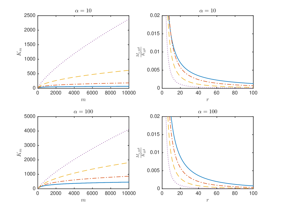
Figure 1: $K_{m}$ and $\frac{M_{r,10^{4}}}{K_{10^{4}}}$ under $P\sim\text{NGGP}(\alpha,\sigma,\nu)$: $\sigma=0$ (blue -), $\sigma=.25$ (red -.), $\sigma=.5$ (yellow –) $\sigma=.75$ (purple :)

3.2 The CMS-NIGP

Because of its unicity in combining a power-law tail behaviour with both a restriction property and a finite-dimensional projective property, the NIGP prior comes as a “forced" choice within our problem of extending the BNP approach of Cai et al., (2018) to deal with power-law data streams. While this choice limits the flexibility of tuning the prior to the power-law degree of the data, in the sense that the NIGP prior is defined as a NGGP prior with $\sigma=1/2$, it is still a sensible choice of practical interest in applications. In particular, if one were forced to choose a single value for $\sigma\in(0,1)$, without information on the power-law degree of the data, $\sigma=1/2$ would arguably be a sensible and safe choice. Hereafter, we assume that tokens in a stream $X_{1:m}$ are modeled as random samples from the NIGP, i.e.,

$$X_{1:m}\mid P \,\stackrel{{\scriptstyle\mbox{{iid}}}}{{\sim}}\,P$$

$$P \,\sim\,\text{NIGP}(\alpha,\nu)$$

for $m\geq 1$. Tokens $X_{i}$’s are hashed through a collection of hash functions $h_{1},\ldots,h_{N}$ drawn uniformly at random from a pairwise independent hash family $\mathcal{H}$ which, for mathematical convenience, it is assumed to be perfectly random. Under this BNP setting, we combine the predictive distribution of the NIGP with both its restriction property and the finite-dimensional projective property to develop a learning-augmented CMS under power-law data streams. This is referred to as the CMS-NIGP. In particular, we show that, a point query induces the posterior distribution for the frequency $f_{v}$ of a token of type $v$ in $X_{1:m}$, given the hashed frequencies $\{C_{n,h_{n}(v)}\}_{n\in[N]}$, for $v\in\mathcal{V}$. CMS-NIGP estimates of $f_{v}$ are obtained as suitable functionals of the posterior distribution, e.g. mode, mean, median.

The predictive distribution of $P\sim\text{NIGP}(\alpha,\nu)$, i.e. Equation (8) with $\sigma=1/2$, induces the conditional distribution of $f_{v}$, given $\mathbf{M}_{m}$. However, since we have only access to the hashed frequencies $\{C_{n,h_{n}(v)}\}_{n\in[N]}$, the object of interest is in the distribution $p_{f_{v}}(m,\alpha)$ of $f_{v}$. Therefore $\mathbf{M}_{m}$ must be marginalized out, under the NIGP prior, from the conditional distribution of $f_{v}$ given $\mathbf{M}_{m}$. That is, the distribution of $f_{v}$ is obtained as

$$p_{f_{v}}(\ell;m,\alpha)=\text{Pr}[f_{v}=\ell]$$

$$\quad=\sum_{\mathbf{m}\in\mathcal{M}_{k,m}}\text{Pr}[X_{m+1}\in\mathbf{v}_{\ell}\mid\mathbf{M}_{m}=\mathbf{m}]\text{Pr}[\mathbf{M}_{m}=\mathbf{m}]$$

for $\ell=0,1,\ldots,m$, where the predictive distribution $\text{Pr}[X_{m+1}\in\mathbf{v}_{\ell}\mid\mathbf{M}_{m}=\mathbf{m}]$ arises from (8) with $\sigma=1/2$, and the distribution $\text{Pr}[\mathbf{M}_{m}=\mathbf{m}]$ arises from (7) with $\sigma=1/2$. The next proposition combines (8) and (7) with $\sigma=1/2$ to compute the distribution $p_{f_{v}}(\ell;m,\alpha)$. In this respect, we exploit the fact that the predictive distribution of the NGGP is a function of simple sufficient statistics of the data stream $X_{1:m}$, i.e. the statistics $K_{n}$ and $(K_{n},M_{r,m})$ for $r=1,\ldots,m$. This peculiar feature of the NGGP (Bacallado et al.,, 2017) prior allows to obtain a workable expression, from a purely computational perspective, of $p_{f_{v}}(\ell;m,\alpha)$. See Appendix E.

Proposition 2.

For any $m\geq 1$, let $X_{1:m}$ denote a random sample of tokens from $P\sim\text{NIGP}(\alpha,\nu)$. Then,

$$p_{f_{v}}(\ell;m,\alpha)=\begin{cases}\frac{{m\choose\ell}e^{\alpha}\alpha}{\pi}\\ \quad\times\int_{0}^{1}K_{-1}\left(\frac{\alpha}{\sqrt{x}}\right)\frac{x^{m-\ell-1}}{(1-x)^{-\frac{1}{2}-\ell+1}}\mathrm{d}x\\ \quad\quad\quad\quad\quad\quad\quad\quad\ell=0,1,\ldots,m-1\\[11.38092pt] \frac{2^{m}\alpha\left(\frac{1}{2}\right)_{(m)}}{\Gamma(m+1)}\\ \quad\times\int_{0}^{+\infty}\frac{x^{m}\text{e}^{-\alpha(\sqrt{1+2x}-1)}}{(1+2x)^{m+1/2}}\mathrm{d}x\\ \quad\quad\quad\quad\quad\quad\quad\quad\ell=m,\end{cases}$$ (11)

where $K_{-1}(\cdot)$ is the modified Bessel function of the second type, or Macdonald function, with parameter $-1$.

Uniformity of the hash function $h\sim\mathcal{H}$ implies that each hash function $h_{n}$ induces a $J$-partition of $\mathcal{V}$, say $\{B_{h_{n},1},\ldots,B_{h_{n},J}\}$, and the measure with respect to $P\sim\text{NIGP}(\alpha,\nu)$ of each $B_{h_{n},j}$ is $1/J$. By the restriction property of the NIGP, the hash function $h_{n}$ turns a global $P\sim\text{NIGP}(\alpha,\nu)$ that governs the distribution of $X_{1:m}$ into a collection of bucket-specific $P_{j}\sim\text{NIGP}(\alpha/J,J\nu_{B_{h_{n},j}})$, for $j=1,\ldots,J$, that govern the distribution of the sole tokens that hashed there. This, combined Proposition 2, leads to the posterior distribution, for the single hash function $h_{n}$, of $f_{v}$ given $C_{n,h_{n}(v)}$, i.e.,

$$\text{Pr}[f_{v}=\ell\,|\,C_{n,h_{n}(v)}=c_{n,h_{n}(v)}]=p_{f_{v}}\left(\ell;c_{n,h_{n}(v)},\frac{\alpha}{J}\right)$$ (12)

for $\ell=0,1,\ldots,c_{n,h_{n}(v)}$ and $n\in[N]$. Then, the posterior distribution of $f_{v}$ given $\{C_{n,h_{n}(v)}\}_{n\in[N]}$ follows from the posterior distribution (12) by exploiting the independence assumption of $\mathcal{H}$ and by Bayes theorem. This posterior distribution, which is reported in the next theorem, is the core of the CMS-NIGP. See Appendix E.

Theorem 3.

Let $h_{1},\ldots,h_{N}$ be hash functions drawn at random from a truly random hash family $\mathcal{H}$. For any $m\geq 1$, let $X_{1:m}$ be a random sample of tokens from $P\sim\text{NIGP}(\alpha,\nu)$ and let $\{C_{n,h_{n}(v)}\}_{n\in[N]}$ be the hashed frequencies induced form $X_{1:m}$ through $h_{1},\ldots,h_{N}$, i.e. $C_{n,h_{n}(v)}=\sum_{1\leq i\leq m}\bm{1}_{h_{n}(X_{i})}(h_{n}(v))$ for $n\in[N]$ and $v\in\mathcal{V}$. Then, the posterior distribution of $f_{v}$, given $\{C_{n,h_{n}(v)}\}_{n\in[N]}$, is

$$\text{Pr}[f_{v}=\ell\mid\{C_{n,h_{n}(v)}\}_{n\in[N]}=\{c_{n,h_{n}(v)}\}_{n\in[N]}]$$ (13)

$$\quad\propto\prod_{n\in[N]}\begin{cases}\frac{{c_{n,h_{n}(v)}\choose\ell}e^{\frac{\alpha}{J}}\alpha}{J\pi}\\ \quad\times\int_{0}^{1}K_{-1}\left(\frac{\alpha}{J\sqrt{x}}\right)\frac{x^{c_{n,h_{n}(v)}-\ell-1}}{(1-x)^{-\frac{1}{2}-\ell+1}}\mathrm{d}x\\ \quad\quad\quad\quad\quad\quad\quad\ell=0,1,\ldots,c_{n,h_{n}(v)}-1\\[11.38092pt] \frac{2^{c_{n,h_{n}(v)}}\alpha\left(\frac{1}{2}\right)_{(c_{n,h_{n}(v)})}}{J\Gamma(c_{n,h_{n}(v)}+1)}\\ \quad\times\int_{0}^{+\infty}\frac{x^{c_{n,h_{n}(v)}}e^{-\frac{\alpha}{J}(\sqrt{1+2x}-1)}}{(1+2x)^{c_{n,h_{n}(v)}+1/2}}\mathrm{d}x\\ \quad\quad\quad\quad\quad\quad\quad\ell=c_{n,h_{n}(v)},\end{cases}$$

where $K_{-1}(\cdot)$ is the modified Bessel function of the second type, or Macdonald function, with parameter $-1$.

While computing the posterior distribution of $f_{v}$ is more than what is required from the classical CMS, it leads to two main advantages: i) the posterior distribution of $f_{v}$ allows to compute different CMS estimates of $f_{v}$ according to the specification of suitable loss functions, e.g. posterior mean under a quadratic loss, posterior median under the absolute loss, posterior mode under the $0$-$1$ loss; ii) the posterior distribution of $f_{v}$ provides a natural tool to quantify uncertainty of CMS estimates, e.g. via the posterior variance or, in general, via credible intervals arising from suitable concentration inequalities. With respect to i), Cai et al., (2018) showed that the posterior mode recovers the CMS estimate, and they applied the posterior mean to improve CMS estimates of low-frequency tokens. In our context of power-law data streams, we will consider the posterior mean, which is shown to provide better estimates of low-frequency tokens. With respect to ii), to the best of our knowledge, there are no studies investigating the problem of assessing uncertainty of CMS estimates. The BNP approach improves over CMS’s algorithms, by providing with a natural tool, i.e. the posterior distribution, for quantifying uncertainty of CMS estimates.

To conclude our posterior analysis of $f_{v}$, it remains to estimate the prior’s parameter $\alpha>0$ from the collection of hashed frequencies. In particular, this step requires the distribution of $\{\mathbf{C}_{n}\}_{n\in[N]}$, that is the likelihood function of the hashed frequencies. According to the finite-dimensional projective property of the NIGP prior, for a single hash function $h_{n}$ the distribution of the hashed frequencies $\mathbf{C}_{n}$ is obtained by integrating the normalized IG distribution (6) with parameter $(\alpha/J,\ldots,\ldots,\alpha/J)$ against the multinomial counts $(\mathbf{c}_{n})$. Then, the distribution of $\{\mathbf{C}_{n}\}_{n\in[N]}$ follows by the independence assumption of the hash family $\mathcal{H}$. That is,

$$\text{Pr}[\{\mathbf{C}_{n}\}_{n\in[N]}=\{\mathbf{c}_{n}\}_{n\in[N]}]$$ (14)

$$\quad=\prod_{n\in[N]}\frac{m\left(\frac{\alpha}{J}\right)^{m+\frac{J}{2}}\text{e}^{\alpha}}{(\pi/2)^{\frac{J}{2}}\prod_{j=1}^{J}c_{n,j}!}$$

$$\quad\quad\times\int_{0}^{+\infty}\frac{x^{m-1}\prod_{j=1}^{J}K_{c_{n,j}-\frac{1}{2}}\left(\frac{\left(\frac{\alpha}{J}\right)}{(1+2x)^{-1/2}}\right)}{(1+2x)^{\frac{m}{2}-\frac{J}{4}}}\mathrm{d}x.$$

See Appendix F. Equation (14) provides an explicit expression of the likelihood function of the hashed frequencies $\{\mathbf{c}_{n}\}_{n\in[N]}$, and thus it allows for estimating the parameter $\alpha$. Here, we adopt an empirical Bayes approach to estimate $\alpha$: we maximize, with respect to $\alpha$, the likelihood function of the hashed frequencies. Alternatively, a fully Bayesian approach can be considered by placing a prior distribution on $\alpha$. The maximization of the likelihood function is performed by evaluating (14) on a grid of exponentially spaced values, which gives an initial bracketing of the maximum. Then, we apply the golden section search derivative-free optimization algorithm (Press et al.,, 2007) to maximize (14) up to a given absolute tolerance for $\alpha$. See Appendix F.

4 Experiments

We apply the CMS-NIGP to synthetic data and to real data. For the CMS-NIGP estimator of $f_{v}$, we consider the posterior mean $\hat{f}_{v}^{\text{{(NIGP)}}}$, which follows from: i) the maximization of (14) with respect to the parameter $\alpha$ for the given data stream of tokens; ii) the evaluation, under the selected (optimal) $\alpha$, of (13) for the given data stream of tokens. To ensure numerical stability in float64, it is imperative to work in log-space and employ the log-sum-exp trick for all summations, including the quadratures to evaluate integrals. In general, the function $K_{\nu}(x)$ is difficult to evaluate for an arbitrary real-valued $\nu$. Hoverer, for the special case $\nu=c_{n,j}-1/2$ considered in (14), $K_{c_{n,j}-1/2}(x)$ admits a finite sum representation that simplify its evaluation. See Appendix F. In (13) instead $\nu$ is integer-valued and numerically accurate implementations are available (Stan and Boost C++). We checked that the number of employed quadrature points resulted in converged numerical estimates, and that the evaluations of (13) passed basic sanity checks. The computational complexity for evaluating (14) directly is $\mathcal{O}(NQJ)$, where $Q$ is the number of quadrature points; we reduced this quantity by caching the evaluations of $K_{c_{n,j}-1/2}$ for each step of the optimization. Instead the evaluation of (13) has $\mathcal{O}(NQ\min_{n}{c_{n,h_{n}(v)}})$ computational complexity. The evaluation of (13) and (14) have been performed on a MacBook Pro, and it takes about ten minutes.

We compare the CMS-NIGP estimator $\hat{f}_{v}^{\text{{(NIGP)}}}$ with respect to: i) the CMS estimator $\hat{f}_{v}^{\text{{(CMS)}}}$ in Cormode and Muthukrishnan, 2005a , namely the minimum hashed frequency based on $N$ hash functions; ii) the CMS-DP estimator $\hat{f}_{v}^{\text{{(DP)}}}$ of Cai et al., (2018) corresponding to the posterior mean under the DP prior. We also consider the count-mean-min (CMM) estimator $\hat{f}_{v}^{\text{{(CMM)}}}$ discussed in the work of Goyal et al., (2012). The CMM relies on the same summary statistics, i.e. the buckets $\{\mathbf{C}_{n}\}_{n\in[N]}$, applied in the CMS, CMS-DP and CMS-NIGP. This facilitates the implementation of a fair comparison among estimators, since the storage requirement and sketch update complexity are unchanged. In particular, Goyal et al., (2012) shows that the CMM estimator stands out in the estimation of low-frequency tokens (see Figure 1 of Goyal et al., (2012)), which is a desirable feature in the context of natural language processing where it is common the power-law behaviour of the data stream of tokens. Hereafter, we compare estimators $\hat{f}_{v}^{\text{{(NIGP)}}}$, $\hat{f}_{v}^{\text{{(DP)}}}$, $\hat{f}_{v}^{\text{{(CMS)}}}$ and $\hat{f}_{v}^{\text{{(CMM)}}}$ in terms of the MAE (mean absolute error) between true frequencies and their corresponding estimates. Because of the limitation of page space, the comparison of $\hat{f}_{v}^{\text{{(NIGP)}}}$ with respect to $\hat{f}_{v}^{\text{{(CMS)}}}$ and $\hat{f}_{v}^{\text{{(CMM)}}}$ on synthetic data is reported in Appendix G. The comparison of $\hat{f}_{v}^{\text{{(NIGP)}}}$ with respect to $\hat{f}_{v}^{\text{{(CMS)}}}$ on real data is also in Appendix G.

We consider datasets of tokens simulated from Zipf’s distribution with (exponent) parameter $s>1$, denoted by $\mathcal{Z}_{s}$. The parameter $s$ controls the tail behaviour of the Zipf’s distribution: the smaller $s$ the heavier is the tail of the distribution, i.e., the smaller $s$ the larger the fraction of symbols with low-frequency tokens. Here, we generate synthetic datasets of $m=500.000$ tokens from a Zipf’s distributions with parameter $s=1.3,\,1.6,\,1.9,\,2.2,\,2.5$. We make use of a $2$-universal hash family, with the following pairs of hashing parameters: i) $J=320$ and $N=2$; ii) $J=160$ and $N=4$. Table 1 and Table 2 reports the MAE of the estimators $\hat{f}_{v}^{\text{{(DP)}}}$ and $\hat{f}_{v}^{\text{{(NIGP)}}}$. From Table 1 and Table 2, it is clear that $\hat{f}_{v}^{\text{{(NIGP)}}}$ has a remarkable better performance than $\hat{f}_{v}^{\text{{(DP)}}}$ in the estimation of low-frequency tokens. In particular, for both Table 1 and Table 2, if we consider the bin of low-frequencies $(0,32]$ the MAE of $\hat{f}_{v}^{\text{{(NIGP)}}}$ is alway smaller than the MAE of $\hat{f}_{v}^{\text{{(DP)}}}$, i.e. $\hat{f}_{v}^{\text{{(NIGP)}}}$ outperforms $\hat{f}_{v}^{\text{{(DP)}}}$. This behaviour becomes more and more evident as the parameter $s$ decreases, that is the heavier is the tail of the distribution the more the estimator $\hat{f}_{v}^{\text{{(NIGP)}}}$ outperforms the estimator $\hat{f}_{v}^{\text{{(DP)}}}$. In particular, for dataset $\mathcal{Z}_{1.5}$ the CMS-NIGP outperforms the CMS-DP for tokens with frequency smaller than 256, whereas for dataset $\mathcal{Z}_{2.5}$ the CMS-NIGP outperforms the CMS-DP for tokens with frequency smaller than 16.

A comparison between $\hat{f}_{v}^{\text{{(NIGP)}}}$, $\hat{f}_{v}^{\text{{(CMS)}}}$ and $\hat{f}_{v}^{\text{{(CMM)}}}$ is reported in Appendix G. This comparison reveals that the CMS-NIGP outperforms the CMS in the estimation of low-frequency tokens for both the choices of hashing parameters, whereas the CMS-NIGP outperforms the CMM in the estimation of low-frequency token for the choice of hashing parameters $J=160$ and $N=4$. In general, from our experiments it emerges that $\hat{f}_{v}^{\text{{(NIGP)}}}$ underestimates large-frequency tokens. To explain this underestimation phenomenon, we observe that the posterior distribution $p_{f_{v}}(\ell;c_{n,h_{n}(v)},\alpha/J)$ in (12) is a decreasing function of $\ell\in\{1,2,\ldots,m\}$. In other terms, the posterior distribution of $f_{v}$ assigns more probability mass to small values of $f_{v}$. Such a decreasing behaviour of $p_{f_{v}}(\ell;c_{n,h_{n}(v)},\alpha/J)$, which is is inherited from the predictive distribution of the NIGP prior, provides an intuitive explanation of the empirical evidence that the larger $v$ the more $\hat{f}_{v}^{\text{{(NIGP)}}}$ underestimates $f_{v}$, i.e. for any parameter $s=1.3,\,1.6,\,1.9,\,2.2,\,2.5$ of Zipf’s distribution the MAE increases along the rows of Table 1 and Table 2. This underestimation phenomenon for large $v$ becomes more evident as $s$ becomes larger, namely as the tail of Zipf’s distribution becomes lighter and hence the fraction of symbols with low-frequency becomes smaller. For instance, we observe that for the bin $(128,256]$ the MAE for $s=2.5$ is larger than the MAE for $s=1.3$.

We also present an application of the CMS-NIGP to textual datasets, for which the distribution of words is typically a power-law distribution. See Clauset et al., (2009) and references therein. Here, we consider the 20 Newsgroups dataset (http://qwone.com/~jason/20Newsgroups/) and the Enron dataset (https://archive.ics.uci.edu/ml/machine-learning-databases/bag-of-words/). The 20 Newsgroups dataset consists of $m=2.765.300$ tokens with $k=53.975$ distinct tokens, whereas the Enron dataset consists of $m=6412175$ tokens with $k=28102$ distinct tokens. Following experiments in Cai et al., (2018), we make use of a $2$-universal hash family, with the following hashing parameters: i) $J=12000$ and $N=2$; ii) $J=8000$ and $N=4$. By means the goodness of fit test proposed in Clauset et al., (2009), we found that the 20 Newsgroups and Enron datasets fit with a power-law distribution with exponent $s=2.3$ and $s=2.1$, respectively. Table 3 reports the MAE of $\hat{f}_{v}^{\text{{(DP)}}}$ and $\hat{f}_{v}^{\text{{(NIGP)}}}$ applied to the 20 Newsgroups dataset and to the Enron dataset. Results of Table 3 confirms the behaviour observed in Zipf’ synthetic data. That is, $\hat{f}_{v}^{\text{{(NIGP)}}}$ outperforms $\hat{f}_{v}^{\text{{(DP)}}}$ for low-frequency tokens, whereas $\hat{f}_{v}^{\text{{(DP)}}}$ of Cai et al., (2018) has a better performance than $\hat{f}_{v}^{\text{{(NIGP)}}}$ for high-frequency tokens. Table 3 also contains a comparison with respect to $\hat{f}_{v}^{\text{{(CMM)}}}$, revealing that $\hat{f}_{v}^{\text{{(NIGP)}}}$ is competitive with $\hat{f}_{v}^{\text{{(CMM)}}}$ in the estimation of low-frequency tokens both the choices of hashing parameters.

Table 1: Synthetic data: MAE for $\hat{f}_{v}^{\text{{(NIGP)}}}$ and $\hat{f}_{v}^{\text{{(DP)}}}$, case $J=320,N=2$

	$\mathcal{Z}_{1.3}$		$\mathcal{Z}_{1.6}$		$\mathcal{Z}_{1.9}$		$\mathcal{Z}_{2.2}$		$\mathcal{Z}_{2.5}$
Bins $v$	$\hat{f}_{v}^{\text{{(DP)}}}$	$\hat{f}_{v}^{\text{{(NIGP)}}}$	$\hat{f}_{v}^{\text{{(DP)}}}$	$\hat{f}_{v}^{\text{{(NIGP)}}}$	$\hat{f}_{v}^{\text{{(DP)}}}$	$\hat{f}_{v}^{\text{{(NIGP)}}}$	$\hat{f}_{v}^{\text{{(DP)}}}$	$\hat{f}_{v}^{\text{{(NIGP)}}}$	$\hat{f}_{v}^{\text{{(DP)}}}$	$\hat{f}_{v}^{\text{{(NIGP)}}}$
(0,1]	1,057.61	231.31	626.85	134.75	306.70	65.71	51.38	12.91	32.43	7.16
(1,2]	1,194.67	287.43	512.43	119.22	153.57	37.03	288.27	61.87	47.84	9.88
(2,4]	1,105.16	262.18	472.59	95.78	2,406.00	353.73	133.31	26.90	53.97	10.09
(4,8]	1,272.02	302.89	783.88	175.10	457.57	83.30	117.76	21.58	69.47	14.28
(8,16]	1,231.63	257.08	716.52	136.66	377.99	66.44	411.21	77.39	80.43	20.15
(16,32]	1,252.18	248.41	829.17	190.05	286.98	41.99	501.00	90.29	9.61	15.36
(32,64]	1,309.14	284.12	780.70	139.52	413.95	67.30	216.84	48.00	9.89	28.90
(64,128]	1,716.76	312.59	946.20	125.07	1,869.23	353.10	63.05	65.91	13.38	66.18
(128,256]	1,102.96	97.91	1,720.49	273.50	199.87	110.32	45.98	130.94	17.03	125.75

Table 2: Synthetic data: MAE for $\hat{f}_{v}^{\text{{(NIGP)}}}$ and $\hat{f}_{v}^{\text{{(DP)}}}$, case $J=160,N=4$

	$\mathcal{Z}_{1.3}$		$\mathcal{Z}_{1.6}$		$\mathcal{Z}_{1.9}$		$\mathcal{Z}_{2.2}$		$\mathcal{Z}_{2.5}$
Bins $v$	$\hat{f}_{v}^{\text{{(DP)}}}$	$\hat{f}_{v}^{\text{{(NIGP)}}}$	$\hat{f}_{v}^{\text{{(DP)}}}$	$\hat{f}_{v}^{\text{{(NIGP)}}}$	$\hat{f}_{v}^{\text{{(DP)}}}$	$\hat{f}_{v}^{\text{{(NIGP)}}}$	$\hat{f}_{v}^{\text{{(DP)}}}$	$\hat{f}_{v}^{\text{{(NIGP)}}}$	$\hat{f}_{v}^{\text{{(DP)}}}$	$\hat{f}_{v}^{\text{{(NIGP)}}}$
(0,1]	2,206.09	0.9	1,254.85	0.25	420.76	0.18	153.20	0.32	56.08	0.38
(1,2]	2,333.06	0.5	1,326.71	0.70	549.12	0.82	180.71	1.24	47.48	1.45
(2,4]	2,266.35	1.3	1,267.97	2.47	482.45	2.53	182.18	2.66	56.87	2.74
(4,8]	2,229.22	4.6	1,371.27	4.67	538.91	5.28	250.32	5.96	50.30	5.42
(8,16]	2,207.42	10.5	1,159.29	10.68	487.69	10.86	245.09	10.28	23.70	11.75
(16,32]	2,279.80	20.7	1,211.41	19.21	529.77	22.08	293.68	21.57	24.41	23.37
(32,64]	2,301.99	42.6	1,280.17	43.14	632.45	42.64	118.26	44.49	30.95	44.03
(64,128]	2,241.57	92.2	1,112.41	94.43	419.42	95.19	177.61	95.10	28.78	93.34
(128,256]	2,235.40	170.0	1,133.85	173.87	522.21	185.83	128.09	180.41	31.46	179.51

Table 3: Real data: MAE for $\hat{f}_{v}^{\text{{(NIGP)}}}$, $\hat{f}_{v}^{\text{{(DP)}}}$ and $\hat{f}_{v}^{\text{{(CMM)}}}$

	$J=12000$ and $N=2$						$J=8000$ and $N=4$
	20 Newsgroups			Enron			20 Newsgroups			Enron
Bins $v$	$\hat{f}_{v}^{\text{{(DP)}}}$	$\hat{f}_{v}^{\text{{(NIGP)}}}$	$\hat{f}_{v}^{\text{{(CMM)}}}$	$\hat{f}_{v}^{\text{{(DP)}}}$	$\hat{f}_{v}^{\text{{(NIGP)}}}$	$\hat{f}_{v}^{\text{{(CMM)}}}$	$\hat{f}_{v}^{\text{{(DP)}}}$	$\hat{f}_{v}^{\text{{(NIGP)}}}$	$\hat{f}_{v}^{\text{{(CMM)}}}$	$\hat{f}_{v}^{\text{{(DP)}}}$	$\hat{f}_{v}^{\text{{(NIGP)}}}$	$\hat{f}_{v}^{\text{{(CMM)}}}$
(0,1]	46.39	11.34	5.41	12.20	3.00	0.90	53.39	0.39	4.50	70.98	0.41	51.00
(1,2]	16.60	3.53	2.16	13.80	3.06	2.00	30.49	1.40	2.00	47.38	1.47	27.20
(2,4]	38.40	7.71	7.91	61.49	12.55	9.90	32.49	2.70	4.80	52.49	3.25	3.90
(4,8]	59.39	10.40	35.70	88.39	17.36	17.32	38.69	5.97	6.23	53.08	6.17	10.50
(8,16]	54.29	11.34	45.40	23.40	4.58	9.52	25.29	11.97	13.50	56.98	11.28	22.20
(16,32]	17.80	9.85	20.99	55.09	11.58	21.00	24.99	21.25	21.60	89.98	19.82	20.60
(32,64]	40.79	25.65	58.86	128.48	39.46	134.47	39.69	42.81	39.22	108.37	47.07	61.38
(64,128]	25.99	57.95	91.59	131.08	54.42	110.27	22.09	91.06	86.32	55.67	87.32	66.50
(128,256]	13.59	126.07	186.92	50.68	119.04	140.43	25.79	205.58	183.96	80.76	178.23	90.20

5 Discussion

Under the BNP approach to CMS of Cai et al., (2018), the restriction property of the DP is critical to compute the posterior distribution of a point query, given the hashed frequencies, whereas the finite-dimensional projective property of the DP is desirable for ease of estimating prior’s parameters since it provides the likelihood function of the hashed frequencies. The NIGP prior is the sole discrete nonparametric prior with power-law behaviour that satisfies both the restriction property and the finite-dimensional projective property. This made the NIGP a somehow "forced" prior choice for our problem of extending the work of Cai et al., (2018) under power-law data streams. By relying on the restriction property and the finite-dimensional projective property of the NIGP, in this paper we have introduced the CMS-NIGP, which is a learning-augmented CMS under power-law data streams of token. The CMS-NIGP exploits BNP modeling to incorporate into the CMS, through the NIGP prior, a sensible power law behavior for the data stream. CMS-NIGP estimates of a point query are obtained as functionals, e.g. mean, mode, median, of the posterior distribution of the point query given the stored hashed frequencies. Applications to synthetic and real data have showed that the CMS-NIGP outperforms the CMS and the CMS-DP in the estimation of low-frequency tokens. The flaw of the CMS in the estimation of low-frequency token is quite well known, especially in the context of natural language processing (Goyal et al.,, 2012, 2009; Pitel and Fouquier,, 2015), and the CMS-NIGP is a new proposal to compensate for this flaw. In particular, the CMS-NIGPS results to be competitive with the CMM of Goyal et al., (2012) in the estimation of low-frequency token.

The NGGP (James,, 2002; Prünster,, 2002; Lijoi et al.,, 2007) and the generalized negative Binomial process (GNBP) of (Zhou et al.,, 2016) are examples of nonparametric priors with power-law behaviour, and we have considered them before turning to the NIGP. Both the NGGP and the GNBP have the restriction property which, however, leads to estimators of a point query that are more involved from a mathematical/computational perspective than estimators under the NIGP prior. See Appendix E. Both the NGGP and the GNBP do not have the finite-dimensional projective property. The lack of the finite-dimensional projective property makes impractical the use of the likelihood function of the hashed frequencies and, in addition, the complicated form of the predictive distributions induced by the NGGP the GNBP makes hard to apply likelihood-free methods to estimate prior’s parameters. We are aware that the NIGP prior limits the flexibility of tuning the prior to the power-law degree of the data, in the sense that the NIGP is defined as a NGGP with $\sigma=1/2$. However, we believe that a NIGP prior is still a sensible choice of practical interest, especially in light of the fact that estimating $\sigma$ under the NGGP prior is a difficult task (Lijoi et al.,, 2007). Moreover, if one were forced to choose a specific value for $\sigma\in(0,1)$, without any information on the power-law degree of the data, $\sigma=1/2$ would arguably be a sensible and safe choice.

Many fruitful directions for future work remain open, especially with respect to the use of the BNP approach to develop learning-augmented CMSs that allows for adapting to the power-law degree of the data stream of tokens. Moreover, based on the promising empirical results of the BNP approach to CMS, we also encourage research to extend the BNP approach to other queries, e.g., range queries, inner product queries. This line of research would broaden the range of applications of the CMS, especially for data streams with power-law behaviour.

6 Acknowledgment

Stefano Favaro is also affiliated to IMATI-CNR “Enrico Magenes" (Milan, Italy). Emanuele Dolera and Stefano Favaro received funding from the European Research Council (ERC) under the European Union’s Horizon 2020 research and innovation programme under grant agreement No 817257. Emanuele Dolera and Stefano Favaro gratefully acknowledge the financial support from the Italian Ministry of Education, University and Research (MIUR), “Dipartimenti di Eccellenza" grant agreement 2018-2022.

References

- Aamand et al., (2019) Aamand, A., Indyk, P., and Vakilian, A. (2019). (learned) frequency estimation algorithms under Zipfian distribution. arXiv preprint arXiv:1908.05198.
- Aggarwal and Yu, (2010) Aggarwal, C. and Yu, P. (2010). On classification of high-cardinality data streams. In Proceedings of the 2010 SIAM International Conference on Data Mining.
- Bacallado et al., (2017) Bacallado, S., Battiston, M., Favaro, S., and Trippa, L. (2017). Sufficientness postulates for gibbs-type priors and hierarchical generalizations. Statistical Science, 32:487–500.
- Cai et al., (2018) Cai, D., Mitzenmacher, M., and Adams, R. P. (2018). A Bayesian nonparametric view on count-min sketch. In Advances in Neural Information Processing Systems.
- Clauset et al., (2009) Clauset, A., Shalizi, C. R., and Newman, M. E. (2009). Power-law distributions in empirical data. SIAM Review, 51:661–703.
- (6) Cormode, G. and Muthukrishnan, S. (2005a). An improved data stream summary: the count-min sketch and its applications. Journal of Algorithms, 55:58–75.
- (7) Cormode, G. and Muthukrishnan, S. (2005b). Summarizing and mining skewed data streams. In Proceedings of the 2005 SIAM International Conference on Data Mining.
- Dwork et al., (2010) Dwork, C., Naor, M., Pitassi, T., Rothblum, G., and Yekhanin, S. (2010). Panprivate streaming algorithms. In Proceedings of The First Symposium on Innovations in Computer Science.
- Ferguson, (1973) Ferguson, T. S. (1973). A Bayesian analysis of some nonparametric problems. The Annals of Statistics, pages 209–230.
- Gnedin et al., (2007) Gnedin, A., Hansen, B., and Pitman, J. (2007). Notes on the occupancy problem with infinitely many boxes: general asymptotics and power laws. Probability Surveys, 4:146–171.
- Goyal et al., (2012) Goyal, A., Daumé, H., and Cormode, G. (2012). Sketch algorithms for estimating point queries in nlp. In Proceedings of the Joint Conference on Empirical Methods in Natural Language Processing and Computational NaturalLanguage Learning.
- Goyal et al., (2009) Goyal, A., Daumé, H., and Venkatasubramanian, S. (2009). Streaming for large scale nlp: language modeling. In Proceedings of the Annual Conference of the North American Chapter of the Association for Computational Linguistics.
- Hadjicharalambous et al., (2011) Hadjicharalambous, G., Favaro, S., and Prünster, I. (2011). On a class of distributions on the simplex. Journal of Statistical Planning and Inference, 141:2987–3004.
- Harrison, (2010) Harrison, B. (2010). Move prediction in the game of Go. Ph.D Thesis, Harvard University.
- Hsu et al., (2019) Hsu, C.-Y., Indyk, P., Katabi, D., and Vakilian, A. (2019). Learning-based frequency estimation algorithms. In International Conference on Learning Representations.
- James, (2002) James, L. F. (2002). Poisson process partition calculus with applications to exchangeable models and Bayesian nonparametrics. arXiv preprint arXiv:math/0205093.
- Kingman, (1993) Kingman, J. (1993). Poisson processes. Wiley Online Library.
- Lijoi et al., (2005) Lijoi, A., Mena, R. H., and Prünster, I. (2005). Hierarchical mixture modeling with normalized inverse-Gaussian priors. Journal of the American Statistical Association, 100:1278–1291.
- Lijoi et al., (2007) Lijoi, A., Mena, R. H., and Prünster, I. (2007). Controlling the reinforcement in Bayesian non-parametric mixture models. Journal of the Royal Statistical Society Series B, 69:715–740.
- Lijoi and Prünster, (2010) Lijoi, A. and Prünster, I. (2010). Models beyond the Dirichlet process. In Bayesian Nonparametrics, Hjort, N.L., Holmes, C.C. Müller, P. and Walker, S.G. Eds. Cambridge University Press.
- Pitel and Fouquier, (2015) Pitel, G. and Fouquier, G. (2015). Count-min-log sketch: approximately counting with approximate counters. In Proceedings of the 1st International Symposium on Web Algorithms.
- Pitman, (2003) Pitman, J. (2003). Poisson-Kingman partitions. In Science and Statistics: A Festschrift for Terry Speed. Institute of Mathematical Statistics.
- Pitman, (2006) Pitman, J. (2006). Combinatorial stochastic processes. Lecture Notes in Mathematics. Springer-Verlag.
- Press et al., (2007) Press, W. H., Teukolsky, S. A., Vetterling, W. T., and Flannery, B. P. (2007). Numerical recipes 3rd edition: The art of scientific computing. Cambridge university press.
- Prünster, (2002) Prünster, I. (2002). Random probability measures derived from increasing additive processes and their application to Bayesian statistics. Ph.D Thesis, University of Pavia.
- Regazzini et al., (2003) Regazzini, E., Lijoi, A., and Prünster, I. (2003). Distributional results for means of normalized random measures with independent increments. The Annals of Statistics, 31:560–585.
- Seshadri, (1993) Seshadri, V. (1993). The inverse Gaussian distribution. Oxford University Press.
- Song et al., (2009) Song, H., Cho, T., Dave, V., Zhang, Y., and Qiu, L. (2009). Scalable proximity estimation and link prediction in online social networks. In Proceedings of the 9th ACM SIGCOMM conference on Internet measurement.
- Zhang et al., (2014) Zhang, Q., Pell, J., Canino-Koning, R., Howe, A., and Brown, C. (2014). These are not the k-mers you are looking for: efficient online k-mer counting using a probabilistic data structure. PloS one, 9.
- Zhou et al., (2016) Zhou, M., Favaro, S., and Walker, S. G. (2016). Frequency of frequencies distributions and size-dependent exchangeable random partitions. Journal of the American Statistical Association, 112:1623–1635.