Electronic width of the $\psi(3770)$ resonance interfering with the background

Abstract

Methods for extracting the $\psi(3770)\to e^{+}e^{-}$ decay width from the data on the reaction cross section $e^{+}e^{-}\to D\bar{D}$ are discussed. Attention is drawn to the absence of the generally accepted method for determining $\Gamma_{\psi(3770)e^{+}e^{-}}$ in the presence of interference between the contributions of the $\psi(3770)$ resonance and background. It is shown that the model for the experimentally measured $D$ meson form factor, which satisfies the requirement of the Watson theorem and takes into account the contribution of the complex of the mixed $\psi(3770)$ and $\psi(2S)$ resonances, allows us to uniquely determine the value of $\Gamma_{\psi(3770)e^{+}e^{-}}$ by fitting. The $\Gamma_{\psi(3770)e^{+}e^{-}}$ values found from the data processing are compared with the estimates in the potential models.

I INTRODUCTION

The charmonium state $\psi(3770)$ PDG20 predicted in the mid-seventies is considered as the $1^{3}D_{1}$ state of the $c\bar{c}$ system with small admixtures of $n^{3}S_{1}$ states [mainly $\psi(2S)$] Ei75 ; Ei76 ; Ei04 ; Ei80 ; Ei06 ; Ei08 ; No78 ; Ro01 ; Ro05 ; Ja77 ; HTO84 . In $e^{+}e^{-}$ collisions, the $\psi(3770)$ resonance is observed in the form of the resonant enhancement, with a width of about 30 MeV, located between the $D\bar{D}$ ($2m_{D}\approx 3.739$ GeV) and $D\bar{D}^{*}$ ($m_{D}+m_{D^{*}}\approx 3.872$ GeV) production thresholds. The sizeable width of the $\psi(3770)$ resonance is due to its strong decays into $D\bar{D}$ meson pairs. Indeed, the fraction of the radiative decays $\psi(3770)\to\gamma\chi_{cJ=0,1,2}$, $\gamma\eta_{c}$, $\gamma\eta_{c}(2S)$ is less than 1.5%, and the fraction of the $\psi(3770)\to J/\psi\pi^{+}\pi^{-}$, $J/\psi\pi^{0}\pi^{0}$ and $J/\psi\eta$ decays is less than $0.5\%$ PDG20 . The total width of the Zweig forbidden decays $\psi(3770)\to light\ hadrons$ must be comparable from the theoretical point of view with the corresponding decay widths of the $J/\psi$ and $\psi(2S)$ resonances located under the $D\bar{D}$ threshold. In order of magnitude, it can be about 100 keV, which is less than $0.5\%$ of the total decay width of the $\psi(3770)$ meson. For almost ninety decay channels, $\psi(3770)\to light\ hadrons$ are known only upper limits (some of which are rather high) PDG20 . Only the branching ratio of the decay $\psi(3770)\to\phi\eta$ is definitely known, $\mathcal{B}(\psi(3770)\to\phi\eta)=(3.1\pm 0.7)\times 10^{-4}$ PDG20 .

The charmonium state $\psi(3770)$ was investigated in $e^{+}e^{-}$ collisions by the MARK-I Ra ; Pe , DELCO Ba , MARK-II Sch , BES Ab1 ; Ab2 ; Ab3 ; Ab3a ; Ab4 ; Ab5 ; Ab6 ; Ab7 ; Ab8 , CLEO Be1 ; Do ; Be2 , BABAR Au1 ; Au2 , Belle Pa , and KEDR An2 Collaborations. The $\psi(3770)$ production was also observed in the $B^{+}\to D\bar{D}K^{+}$ decays by the Belle Ch04 ; Br08 , BABAR Au08 ; Le15 , and LHCb Aa20 Collaborations. Full compilation of the $\psi(3770)$ production experiments is contained in the review of the Particle Data Group (PDG) PDG20 . The unusual shape of the $\psi(3770)$ resonance peak, discovered in many experiments Ab3a ; Ab4 ; Ab6 ; Ab7 ; Ab8 ; Au1 ; Au2 ; Pa ; An2 , naturally became the subject of many-sided theoretical analyses (see, for example, Refs. Ya ; LQY ; ZZ ; AS12 ; AS13 ; CZ ; Li ; CL14a ; CL14b ; DMW ; ST ; CG ). The following circumstance is also of additional interest. According to the CLEO data Be1 ; Do ; Be2 , the value of the non-$D\bar{D}$ component in the decay width of the $\psi(3770)$ resonance is negligible. At the same time, the BES analysis Ab2 ; Ab3 ; Ab4 ; Ab5 does not exclude a noticeable non-$D\bar{D}$ component. According to the theoretical estimates He08 ; He10 , the non-$D\bar{D}$ decay branching ratio of $\psi(3770)$ could reach about 5%. The authors of Refs. He08 ; He10 note that this result does not contain evidence in favor of BES or CLEO results, and urge doing more precise measurements on both inclusive and exclusive non-$D\bar{D}$ decays of $\psi(3770)$ in the future. Unfortunately, this contradiction has not yet been resolved. As a result, the PDG PDG20 gives the following value for the $D\bar{D}$ component: $\mathcal{B}(\psi(3770)\to D\bar{D})=[\mathcal{B}(\psi(3770)\to D^{+}D^{-})=(52\pm^{4}_{5})\%]+[\mathcal{B}(\psi(3770)\to D^{0}\bar{D}^{0})=(41\pm 4)\%]=(93\pm^{8}_{9})\%$. Theoretical considerations combined with the CLEO data Be1 ; Do ; Be2 suggest that the dominance of the $\psi(3770)\to D\bar{D}$ decay can be at the level of $97\%-98\%$. In what follows, we will consider $\psi(3770)$ to be an almost elastic resonance coupled to the $D\bar{D}$ decay channels and apply this assumption to describe its line shape and determine its electronic decay width, $\Gamma_{\psi(3770)e^{+}e^{-}}$.

This paper is organized as follows. Section II gives a brief overview of the commonly used methods for describing the $\psi(3770)$ resonance and the definitions of $\Gamma_{\psi(3770)e^{+}e^{-}}$, particularly those selected by the PDG PDG20 for calculations fitting $(0.262\pm 0.018)$ keV and average $(0.256\pm 0.016)$ keV values of $\Gamma_{\psi(3770)e^{+}e^{-}}$. Attention is drawn to the fact that some seemingly natural parametrizations of the cross section $\sigma(e^{+}e^{-}\to D\bar{D})$, taking into account the interference of the $\psi(3770)$ resonance and background, do not allow us to determine the value of $\Gamma_{\psi(3770)e^{+}e^{-}}$ uniquely. In Sec. III, we apply to the description of the reaction cross section $\sigma(e^{+}e^{-}\to D\bar{D})$ the model for the isoscalar form factor of the $D$ meson, which takes into account the contributions of the $\psi(3770)$ and $\psi(2S)$ resonances mixed due to their coupling with the $D\bar{D}$ decay channels. The model satisfies the requirement of the unitarity condition or the Watson theorem Wa52 and allows us to unambiguously determine the value of $\Gamma_{\psi(3770)e^{+}e^{-}}$ from the data by fitting. Our analysis substantially develops the approach proposed in Refs. AS12 ; AS13 by consistently taking into account the finite width corrections in the resonance propagators and clarifying their important role. In Sec. IV, we compare the values of $\Gamma_{\psi(3770)e^{+}e^{-}}$ found from phenomenological data processing with theoretical estimates in potential models and briefly state our conclusions.

II Parametrizations of the $\psi(3770)$ resonance structure

In many experimental works, the cross section of the reaction $e^{+}e^{-}\to D\bar{D}$ in the $\psi(3770)$ resonance region was described with minor modification by the following formula Ra ; Pe ; Ba ; Sch ; Ab1 ; Ab2 ; Ab3 ; Ab3a ; Ab4 ; Ab5 ; Be1 [for short, $\psi(3770)$ is also denoted as $\psi^{\prime\prime}$ below]:

$$\sigma_{\psi^{\prime\prime}}(e^{+}e^{-}\to D\bar{D};\,s)=\frac{12\pi\Gamma_{\psi^{\prime\prime}e^{+}e^{-}}\Gamma_{\psi^{\prime\prime}D\bar{D}}(s)}{(m^{2}_{\psi^{\prime\prime}}-s)^{2}+(m_{\psi^{\prime\prime}}\Gamma^{tot}_{\psi^{\prime\prime}}(s))^{2}},$$ (1)

where $s$ is the invariant mass squared of the $D\bar{D}$ system, $m_{\psi^{\prime\prime}}$, $\Gamma_{\psi^{\prime\prime}e^{+}e^{-}}$, $\Gamma_{\psi^{\prime\prime}D\bar{D}}(s)$, and $\Gamma^{tot}_{\psi^{\prime\prime}}(s)$ are the mass, electronic, $D\bar{D}$, and total decay widths of $\psi^{\prime\prime}$, respectively. The energy-dependent width $\Gamma_{\psi^{\prime\prime}D\bar{D}}(s)$ [dominating in $\Gamma^{tot}_{\psi^{\prime\prime}}(s)$] was taken in the form

$$\Gamma_{\psi^{\prime\prime}D\bar{D}}(s)=G^{2}_{\psi^{\prime\prime}}\left(\frac{p^{3}_{0}(s)}{1+r^{2}p^{2}_{0}(s)}+\frac{p^{3}_{+}(s)}{1+r^{2}p^{2}_{+}(s)}\right),$$ (2)

where $p_{0}(s)$ = $\sqrt{s/4-m^{2}_{D^{0}}}$ and $p_{+}(s)$ = $\sqrt{s/4-m^{2}_{D^{+}}}$ are the $D^{0}$ and $D^{+}$ momenta in the $\psi^{\prime\prime}$ rest frame, $r$ is the $D\bar{D}$ interaction radius BW52 , and $G_{\psi^{\prime\prime}}$ is the coupling constant of the $\psi^{\prime\prime}$ with $D\bar{D}$.

For the solitary $\psi^{\prime\prime}$ resonance, there is no problem with determining $\Gamma_{\psi^{\prime\prime}e^{+}e^{-}}$ by fitting the data using Eqs. (1) and (2). Discrepancy between the values found by different Collaborations ($\Gamma_{\psi^{\prime\prime}e^{+}e^{-}}=345\pm 85$ eV Pe , $180\pm 60$ eV Ba , $276\pm 50$ eV Sch , $279\pm 11\pm 13$ eV Ab4 , $220\pm 50$ eV Ab6 ; PDG20 , $204\pm 3^{+41}_{-27}$ eV Be1 ) is mainly related to the difference in the collected raw data and uncertainties in the cross section normalization.

With increasing accuracy of measurements, there appeared to be indications of an unusual (anomalous) shape of the $\psi(3770)$ peak in the $e^{+}e^{-}\to\psi^{\prime\prime}\to hadrons$ and $e^{+}e^{-}\to\psi^{\prime\prime}\to D\bar{D}$ reaction cross sections, i.e., on possible interference effects that occur directly in the $\psi(3770)$ resonance region Ab3a ; Ab4 ; Ab6 ; Ab7 ; Ab8 ; Au1 ; Au2 ; Pa ; An2 . In particular, there is a deep dip in the $D\bar{D}$ production cross section near $\sqrt{s}\approx 3.81$ GeV Ab3a ; Ab4 ; Au1 ; Au2 ; Pa which strongly distorts the right wing of the $\psi^{\prime\prime}$ resonance. Such a dip is difficult to describe using Eqs. (1) and (2) for a solitary $\psi^{\prime\prime}$ resonance contribution. In Ref AS12 , we showed that the description of the data Ab3a ; Ab4 ; Au1 ; Au2 ; Pa ; Be2 with the use of these formulas turns out to be unsatisfactory for any values of the parameter $r$. In addition, by performing the analytical continuation of the amplitudes $e^{+}e^{-}\to\psi^{\prime\prime}\to D^{0}\bar{D}^{0}$ and $e^{+}e^{-}\to\psi^{\prime\prime}\to D^{+}D^{-}$ corresponding to the parametrizations (1) and (2) below the $D\bar{D}$ thresholds, it is easy to make sure that they have spurious poles and left cuts due to the $P$-wave Blatt and Weisskopf barrier penetration factors, $1/[1+r^{2}p^{2}_{0,+}(s)]$ BW52 . For example, for $r\approx 1\,\mbox{fm}\approx 5\,\mbox{GeV}^{-1}$, the indicated singularities appear at about 20 MeV below the $D\bar{D}$ thresholds. In the next section, we show that taking into account the finite width corrections in the resonance propagators allows us to eliminate these singularities.

If we are not dealing with a solitary resonance, but with a complex of the mixed resonance and background contributions, then a practical question arises about the way of describing it as a whole and the possibilities of adequately determining the individual characteristics of its components. In what follows, we will talk about the process $e^{+}e^{-}\to D\bar{D}$, in which the isoscalar electromagnetic form factor of the $D$ meson $F^{0}_{D}(s)$ is measured. The sum of the $e^{+}e^{-}\to D\bar{D}$ reaction cross sections is expressed in the terms of $F^{0}_{D}(s)$ as follows:

$$\sigma(e^{+}e^{-}\to D\bar{D};\,s)=\frac{8\pi\alpha^{2}}{3s^{5/2}}\left|F^{0}_{D}(s)\right|^{2}\left[p^{3}_{0}(s)+p^{3}_{+}(s)\right]\,,$$ (3)

where $\alpha$ = $e^{2}/4\pi$ = 1/137. Here we neglect the isovector part of the $D$ meson form factor and do not touch on the question about the isospin symmetry breaking. The KEDR Collaboration An2 , analyzing their own data on the $e^{+}e^{-}\to D\bar{D}$ cross section, showed that taking into account the interference between the $\psi(3770)$ resonance and background contributions affects the value^,s resonance parameters and therefore the corresponding results cannot be directly compared with those obtained ignoring this effect. In addition, in Ref. An2 , within the framework of the accepted parametrization for $F^{0}_{D}(s)$, two essentially different solutions were obtained for the production amplitude of the $\psi(3770)$ state and its phase relative to the background (see also ST ). These two solutions lead to the same energy dependence of the $e^{+}e^{-}\to D\bar{D}$ cross section and are indistinguishable by the $\chi^{2}$ criterion. Ambiguities of this type in the interfering resonance parameter determination were found in Ref. Bu (see also Zh ; Yu ). The PDG used one of the KEDR solutions An2 [see Eq. (8) below] to determine the value of $\Gamma_{\psi^{\prime\prime}e^{+}e^{-}}=(0.262\pm 0.018)$ keV PDG20 , together with the above results from other works Ba ; Sch ; Ab4 ; Ab6 ; Be1 (in which the interference was not taken into account).

Let us illustrate the ambiguity of the choice of the resonance parameters with a simple example. Consider a model of the reaction amplitude $e^{+}e^{-}\to h\bar{h}$ (where $h$ and $\bar{h}$ are hadrons), which takes into account the resonance and background contributions;

$$F(E)=\frac{A_{x}e^{i\varphi_{x}}}{M-E-i\Gamma/2}+B_{x}$$ (4)

Here, $E$ is the energy in the $h\bar{h}$ center-of-mass system, $M$ is the mass, $\Gamma$ is the energy-independent width of the resonance, and $A_{x}$, $\varphi_{x}$, and $B_{x}$ are the real parameters. At fixed $M$ and $\Gamma$, there are two solutions for $A_{x}$, $\varphi_{x}$, and $B_{x}$ Bu :

$$\mbox{(I)}\quad A_{x}=A,\ \ B_{x}=B,\ \ \varphi_{x}=\varphi,$$ (5)

$$\mbox{(II)}\quad A_{x}=\sqrt{A^{2}-2AB\Gamma\sin\varphi+B^{2}\Gamma^{2}},\ \ B_{x}=B,\ \ \tan\varphi_{x}=-\tan\varphi+B\Gamma/(A\cos\varphi),\qquad$$ (6)

which yield the same cross section as a function of energy, $\sigma(E)$ = $|F(E)|^{2}$, and different amplitude, $A_{x}$, and phase, $\varphi_{x}$. For example, if $M$ = 3.77 GeV, $\Gamma$ = 0.03 GeV $A$ = 0.045 nb^1/2GeV, $\varphi$ = 0, and $B$ = 1.5 nb^1/2 for solution (I), then, for solution (II), $A_{x}$ = $\sqrt{2}A$ and $\varphi_{x}$ = $\pi/4$. Since $A_{x}\sim\sqrt{\Gamma_{e^{+}e^{-}}\Gamma}$, the values of the electronic decay width of the resonance $\Gamma_{e^{+}e^{-}}$ differ by a factor of two for solutions (I) and (II).

The similar form factor parametrization was used to determine the $\psi(3770)$ resonance parameters in Ref An2 :

$$F^{0}_{D}(s)=F^{\psi(3770)}(s)e^{i\phi}+F^{\mbox{\scriptsize{N.R.}}}(s),$$ (7)

where $F^{\psi(3770)}(s)$ is the Breit-Wigner $P$-wave resonance amplitude, $F^{\mbox{\scriptsize{N.R.}}}(s)$ is the background amplitude, and $\phi$ is their relative phase. $F^{\mbox{\scriptsize{N.R.}}}(s)=F^{\psi(2S)}(s)+F_{0}$ takes into account the contribution of the right wing of the nearest resonance $\psi(2S)$ with the mass of 3.686 GeV and the additional constant contribution $F_{0}$. Two solutions indistinguishable in $\chi^{2}$ are An2 :

$$\mbox{(I)}\quad\Gamma_{\psi^{\prime\prime}e^{+}e^{-}}=160^{+78}_{-58}\,\ \mbox{eV},\quad\phi=(170.7\pm 16.7)^{\circ},$$ (8)

$$\mbox{(II)}\quad\Gamma_{\psi^{\prime\prime}e^{+}e^{-}}=420^{+72}_{-80}\,\ \mbox{eV},\quad\phi=(239.6\pm 8.6)^{\circ}.$$ (9)

Thus, parametrizations of types (4) and (7), preserving at first glance the usual way of determining the individual characteristics of the $\psi^{\prime\prime}$ resonance (for example, its electronic width), do not allow to do this unambiguously by fitting. If one of the values of $\Gamma_{\psi^{\prime\prime}e^{+}e^{-}}$ from Eqs. (8) and (9) agrees with some theoretical estimate of $\Gamma_{\psi^{\prime\prime}e^{+}e^{-}}$, then it does not yet mean the validity of Eq. (7), which contains the phase $\phi$ of unknown origin and does not take into account the transition amplitude between the background and resonance through the common $D\bar{D}$ intermediate states.

However, just in the case of the $\psi^{\prime\prime}$ resonance, the above difficulties can be avoided if we take into account the requirement of the unitarity condition. As noted above, the $\psi^{\prime\prime}$ is the elastic resonance in a good approximation. But in the elastic region (between $D\bar{D}$ and $D\bar{D}^{*}$ thresholds) with a width of about 141 MeV, the unitarity condition requires that the phase of the form factor $F^{0}_{D}(s)$ coincide with the phase $\delta^{0}_{1}(s)$ of the strong $P$-wave $D\bar{D}$ elastic scattering amplitude $T^{0}_{1}(s)=e^{\delta^{0}_{1}(s)}\sin\delta^{0}_{1}(s)$ in the channel with isospin $I=0$, i.e.,

$$F^{0}_{D}(s)=e^{i\delta^{0}_{1}(s)}\mathcal{F}^{0}_{D}(s)\,,$$ (10)

where $\mathcal{F}^{0}_{D}(s)$ and $\delta^{0}_{1}(s)$ are the real functions of energy Wa52 . It is clear that formulas (4) and (7) contradict the unitarity requirement since the phase of the form factor determined by them depends on the ratio of the background and resonance coupling constants with $e^{+}e^{-}$, on which $\delta^{0}_{1}(s)$ is obviously independent.

In the next section, we apply to the description of the data on the reaction $e^{+}e^{-}\to D\bar{D}$ a simple model of the form factor $F^{0}_{D}(s)$, which satisfies the requirement of the unitarity condition for the case of the mixed $\psi^{\prime\prime}$ and $\psi(2S)$ resonances and allows by fitting to uniquely determine the value of $\Gamma_{\psi^{\prime\prime}e^{+}e^{-}}$. Our analysis is an advancement of that which is suggested earlier in AS12 ; AS13 .

III The $D$ meson electromagnetic form factor in the $\psi(3770)$ region

III.1 The solitary $\psi^{\prime\prime}$ resonance

Consider a model that takes into account in the form factor $F^{0}_{D}(s)$, amplitude $T^{0}_{1}(s)$, and the contributions of two resonances, $\psi^{\prime\prime}$ and $\psi(2S)$, that are close to each other, strongly coupled only to $D\bar{D}$ decay channels, and are mixing with each other due to transitions $\psi^{\prime\prime}\to D\bar{D}\to\psi(2S)$ and vice versa. However, we first write down the contribution of $\psi^{\prime\prime}$ to $F^{0}_{D}(s)$ in the spirit of the vector dominance model FN1 ; GS ; RP ; BM , ignoring its mixing with $\psi(2S)$;

$$F^{0}_{D}(s)=F^{\psi^{\prime\prime}}_{D}(s)=\frac{C_{\psi^{\prime\prime}}}{\widetilde{D}_{\psi^{\prime\prime}}(s)}=\frac{C_{\psi^{\prime\prime}}}{m^{2}_{\psi^{\prime\prime}}-s-h_{\psi^{\prime\prime}}(s)-i\sqrt{s}\Gamma_{\psi^{\prime\prime}D\bar{D}}(s)},$$ (11)

where $C_{\psi^{\prime\prime}}$ is an $s$-independent constant, $\widetilde{D}_{\psi^{\prime\prime}}(s)$ is the inverse propagator of $\psi^{\prime\prime}$, and where

$$\Gamma_{\psi^{\prime\prime}D\bar{D}}(s)=\frac{g^{2}_{\psi^{\prime\prime}D\bar{D}}}{6\pi s}\left(\frac{p^{3}_{0}(s)}{1+r^{2}p^{2}_{0}(s)}+\frac{p^{3}_{+}(s)}{1+r^{2}p^{2}_{+}(s)}\right),$$ (12)

is the $\psi^{\prime\prime}\to D\bar{D}$ decay width, where $g_{\psi^{\prime\prime}D\bar{D}}$ is the corresponding coupling constant. The function $h_{\psi^{\prime\prime}}(s)$ describes the contribution of the finite width corrections to the real part of the $\psi^{\prime\prime}$ propagator. Its explicit form is given in Appendix. Near $s=m^{2}_{\psi^{\prime\prime}}$ is the function $h_{\psi^{\prime\prime}}(s)\sim(m^{2}_{\psi^{\prime\prime}}-s)^{2}$. Values $C_{\psi^{\prime\prime}}$, $m_{\psi^{\prime\prime}}$, $g_{\psi^{\prime\prime}D\bar{D}}$, and $r$ are free parameters of the model. To normalize the form factor $F^{\psi^{\prime\prime}}_{D}(s)$ at $s=m^{2}_{\psi^{\prime\prime}}$, we use the relation

$$\sigma_{\psi^{\prime\prime}}(e^{+}e^{-}\to D\bar{D};\,s=m^{2}_{\psi^{\prime\prime}})=\frac{12\pi}{m^{2}_{\psi^{\prime\prime}}}\frac{\Gamma_{\psi^{\prime\prime}e^{+}e^{-}}}{\Gamma_{\psi^{\prime\prime}D\bar{D}}}\,,$$ (13)

where $\Gamma_{\psi^{\prime\prime}D\bar{D}}\equiv\Gamma_{\psi^{\prime\prime}D\bar{D}}(m^{2}_{\psi^{\prime\prime}})$. Then, taking into account Eqs. (3), (11), and (13), we have (up to a sign),

$$C_{\psi^{\prime\prime}}=\sqrt{\frac{9m^{5}_{\psi^{\prime\prime}}\,\Gamma_{\psi^{\prime\prime}e^{+}e^{-}}\Gamma_{\psi^{\prime\prime}D\bar{D}}}{\ 2\alpha^{2}\left(p^{3}_{0}(m^{2}_{\psi^{\prime\prime}})+p^{3}_{+}(m^{2}_{\psi^{\prime\prime}})\right)}}\ .$$ (14)

Putting, by definition, $\Gamma_{\psi^{\prime\prime}e^{+}e^{-}}=4\pi\alpha^{2}g^{2}_{\psi^{\prime\prime}\gamma}/(3m_{\psi^{\prime\prime}}^{3})$, where the constant $g_{\psi^{\prime\prime}\gamma}$ describes the $\psi^{\prime\prime}$ coupling with the virtual $\gamma$ quantum, we can write $C_{\psi^{\prime\prime}}$ in the form:

$$C_{\psi^{\prime\prime}}=g_{\psi^{\prime\prime}\gamma}\,g^{eff}_{\psi^{\prime\prime}D\bar{D}}\,.$$ (15)

The effective coupling constant of the $\psi^{\prime\prime}$ resonance with $D\bar{D}$   $g^{eff}_{\psi^{\prime\prime}D\bar{D}}$ is related to the constant $g_{\psi^{\prime\prime}D\bar{D}}$ from Eq. (12) by the relation

$$g^{eff}_{\psi^{\prime\prime}D\bar{D}}=\sqrt{6\pi m^{2}_{\psi^{\prime\prime}}\Gamma_{\psi^{\prime\prime}D\bar{D}}/[p^{3}_{0}(m^{2}_{\psi^{\prime\prime}})+p^{3}_{+}(m^{2}_{\psi^{\prime\prime}})]}\,.$$ (16)

From Eqs. (11) and (IV)–(A4) it follows that, owing to the finite width corrections in $\widetilde{D}_{\psi^{\prime\prime}}(s)$, the form factor $F^{\psi^{\prime\prime}}_{D}(s)$ has good analytical properties. In particular, it has no any singularities associated with the poles of the functions $1/[1+r^{2}p^{2}_{0,+}(s)]$. In addition, in $F^{\psi^{\prime\prime}}_{D}(s)$ there are absent spurious bound states in the region $0<s<4m^{2}_{D^{+}}$ for $r\geq 0.87$ GeV^-1 (0.174 fm) [i.e., $\widetilde{D}_{\psi^{\prime\prime}}(s)$ does not vanish anywhere in this region].

The fit to the data Ab3a ; Ab4 ; Be2 ; Au1 ; Au2 ; Pa with the use of the solitary $\psi^{\prime\prime}$ resonance model at a fixed value of $r=0.87$ GeV^-1 is shown in Fig. 1. It corresponds to $m_{\psi^{\prime\prime}}=3.772$ GeV, $g_{\psi^{\prime\prime}D\bar{D}}=14.4$ [i.e., $\Gamma_{\psi^{\prime\prime}D\bar{D}}(m^{2}_{\psi^{\prime\prime}})\approx 27.6$ MeV], and $g_{\psi^{\prime\prime}\gamma}=0.245$ GeV² (i.e., $\Gamma_{\psi^{\prime\prime}e^{+}e^{-}}\approx 0.25$ keV). Although the obtained values of the $\psi^{\prime\prime}$ parameters are close to those given by the PDG PDG20 , the fit in itself is unsatisfactory. The corresponding $\chi^{2}=459$ for 84 degrees of freedom. As $r$ increases, the fit becomes even less satisfactory.

With regard to the selected data Ab3a ; Ab4 ; Be2 ; Au1 ; Au2 ; Pa (see Fig. 1), we note the following. These data are the most detailed and accurate available data on the so-called Born cross section (i.e., on the cross section undistorted by initial state radiation). Note that the BES Collaboration Ab3a ; Ab4 measured, in the region up to the $D\bar{D}^{*}$ threshold ($\approx$ 3.872 GeV), the quantity $R(s)$ = $\sigma(e^{+}e^{-}\to hadrons)/\sigma(e^{+}e^{-}\to\mu^{+}\mu^{-})$. The $D\bar{D}$ events were not specially identified. The 62 BES points shown in Fig. 1 correspond to the cross section $(4\pi\alpha^{2}/3s)[R(s)-R_{uds}]$, where $R_{uds}=2.121$ Ab4 describes the background from the light hadron production. This cross section gives a good estimate for $\sigma(e^{+}e^{-}$ $\to$ $D\bar{D})$ in the $\psi(3770)$ region, see the discussion in the Introduction and also in Ref. AS12 . The utilized approximation is not critical for our analysis.

III.2 The $\psi(2S)$ contribution

Let us write the contribution of the state $\psi(2S)$ to $F^{0}_{D}(s)$ by analogy with Eq. (11) in the form

$$F^{0}_{D}(s)=F^{\psi(2S)}_{D}(s)=\frac{C_{\psi(2S)}}{\widetilde{D}_{\psi(2S)}(s)}=\frac{C_{\psi(2S)}}{m^{2}_{\psi(2S)}-s-h_{\psi(2S)}(s)-i\sqrt{s}\Gamma_{\psi(2S)D\bar{D}}(s)}\,,$$ (17)

where $m_{\psi(2S)}=3.6861$ GeV PDG20 . $F^{\psi(2S)}_{D}(s)$ is calculated according to Eqs. (12) and (IV)–(A4), where the index $\psi^{\prime\prime}$ should be replaced everywhere by $\psi(2S)$. The constant $C_{\psi(2S)}$ in Eq. (17) can be represented by analogy with Eq. (15) in the form

$$C_{\psi(2S)}=g_{\psi(2S)\gamma}\,g^{eff}_{\psi(2S)D\bar{D}}\,.$$ (18)

The constant $g_{\psi(2S)\gamma}$ describes the $\psi(2S)$ coupling with the virtual $\gamma$ quantum. From the PDG data PDG20 , $\Gamma_{\psi(2S)e^{+}e^{-}}=2.33$ keV, and the relation $\Gamma_{\psi(2S)e^{+}e^{-}}=4\pi\alpha^{2}g^{2}_{\psi(2S)\gamma}/(3m^{3}_{\psi(2S)})$; thus we get $g_{\psi(2S)\gamma}=\pm 0.723$ GeV².

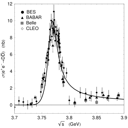
Figure 1: The variant of the solitary $\psi^{\prime\prime}$ resonance model. The curve is the fit using Eqs. (3) and (11)–(15) with the data from BES Ab3a ; Ab4 , CLEO Be2 , $BABAR$ Au1 ; Au2 , and Belle Pa Collaborations for $\sigma(e^{+}e^{-}$ $\to$ $D\bar{D})$. There are 87 points in the fit. For more details on the data see the text and also Ref. AS12 .

As a free parameter for the $\psi(2S)$ contribution, it is convenient to use the proportionality coefficient $z$ between the coupling constants of the $\psi(2S)$ and $\psi^{\prime\prime}$ with $D\bar{D}$:

$$g_{\psi(2S)D\bar{D}}=z\,g_{\psi^{\prime\prime}D\bar{D}}\ \ \ \mbox{and}\ \ \ g^{eff}_{\psi(2S)D\bar{D}}=z\,g^{eff}_{\psi^{\prime\prime}D\bar{D}}.$$ (19)

The relation between $g_{\psi^{\prime\prime}D\bar{D}}$ and $g^{eff}_{\psi^{\prime\prime}D\bar{D}}$ is definite by Eq. (16).

III.3 $D$ meson form factor for the mixed $\psi^{\prime\prime}$ and $\psi(2S)$ states

We now take into account the mixing of $\psi^{\prime\prime}$ and $\psi(2S)$ resonances due to their common decay channels into $D^{0}\bar{D}^{0}$ and $D^{+}D^{-}$. The form factor $F^{0}_{D}(s)$ corresponding to such a $\psi^{\prime\prime}-\psi(2S)$ resonance complex can be written as AS12 ; AS13

$$F^{0}_{D}(s)=\frac{C_{\psi^{\prime\prime}}\Delta_{\psi(2S)}(s)+C_{\psi(2S)}\Delta_{\psi^{\prime\prime}}(s)}{\widetilde{D}_{\psi^{\prime\prime}}(s)\widetilde{D}_{\psi(2S)}(s)-\widetilde{\Pi}^{2}_{\psi^{\prime\prime}\psi(2S)}(s)}\,,$$ (20)

where

$$\Delta_{\psi(2S)}(s)=\widetilde{D}_{\psi(2S)}(s)+z\,\widetilde{\Pi}_{\psi^{\prime\prime}\psi(2S)}(s)\,,$$ (21)

$$\Delta_{\psi^{\prime\prime}}(s)=\widetilde{D}_{\psi^{\prime\prime}}(s)+z^{-1}\,\widetilde{\Pi}_{\psi^{\prime\prime}\psi(2S)}(s)\,,\ \$$ (22)

and $\widetilde{\Pi}_{\psi^{\prime\prime}\psi(2S)}(s)$ is the nondiagonal polarization operator describing the transition $\psi^{\prime\prime}$ $\to$ $D\bar{D}$ $\to$ $\psi(2S)$. The polarization operator $\widetilde{\Pi}_{\psi^{\prime\prime}\psi(2S)}(s)$ is related to the diagonal polarization operator $\Pi_{\psi^{\prime\prime}}(s)$ (see Appendix) by the relation

$$\widetilde{\Pi}_{\psi^{\prime\prime}\psi(2S)}(s)=z\,\Pi_{\psi^{\prime\prime}}(s)+a+s\,b,$$ (23)

where $a$ and $b$ are unknown constants. In order to use the parameters introduced above for the description of solitary $\psi^{\prime\prime}$ and $\psi(2S)$ resonances (fixed $m_{\psi(2S)}$ and $g_{\psi(2S)\gamma}$ and free $m_{\psi^{\prime\prime}}$, $g_{\psi^{\prime\prime}\gamma}$, $g_{\psi^{\prime\prime}D\bar{D}}$, and $g_{\psi(2S)D\bar{D}}$ or $z$) and preserve the meaning of individual characteristics for resonances dressed by mixing, we fix the constants $a$ and $b$ by the conditions

$$\mbox{Re}\,\widetilde{\Pi}_{\psi^{\prime\prime}\psi(2S)}(m^{2}_{\psi(2S)})=0\,,$$ (24)

$$\mbox{Re}\,\widetilde{\Pi}_{\psi^{\prime\prime}\psi(2S)}(m^{2}_{\psi^{\prime\prime}})=0\,.\ \$$ (25)

Note that Eq. (25) keeps the normalization condition (13) for the form factor $F^{0}_{D}(s)$ given by formula (20). Using Eqs. (24) and (25), we find

$$\widetilde{\Pi}_{\psi^{\prime\prime}\psi(2S)}(s)=z\,\left[\Pi_{\psi^{\prime\prime}}(s)-\mbox{Re}\,\Pi_{\psi^{\prime\prime}}(m^{2}_{\psi^{\prime\prime}})+\frac{s-m^{2}_{\psi^{\prime\prime}}}{m^{2}_{\psi^{\prime\prime}}-m^{2}_{\psi(2S)}}\,\mbox{Re}\left(\Pi_{\psi^{\prime\prime}}(m^{2}_{\psi(2S)})-\Pi_{\psi^{\prime\prime}}(m^{2}_{\psi^{\prime\prime}})\right)\right].$$ (26)

Note that the phase of the form factor $F^{0}_{D}(s)$, due to the strong resonant interaction of $D$ mesons, is determined by the phase of the denominator in Eq. (20). The numerator in this formula is the first-degree polynomial in $s$ with real coefficients. It is interesting that in the case under consideration we are faced, perhaps for the first time, with the possibility of the existence of zero in the form factor in the elastic region. As seen from Fig. 1, the data do not contradict the presence of zero in $F^{0}_{D}(s)$ at $\sqrt{s}\approx 3.81$ GeV FN3 .

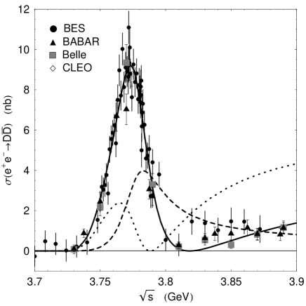
Figure 2: The model of the mixed $\psi^{\prime\prime}$ and $\psi(2S)$ resonances. The solid curve is the fit using Eqs. (3) and (20)–(26) to the data from BES Ab3a ; Ab4 , CLEO Be2 , $BABAR$ Au1 ; Au2 , and Belle Pa Collaborations. The dashed and dotted curves show the contributions to the cross section from the $\psi^{\prime\prime}$ and $\psi(2S)$ production amplitudes proportional to the coupling constants $C_{\psi^{\prime\prime}}$ and $C_{\psi(2S)}$, respectively; see Eq. (20).

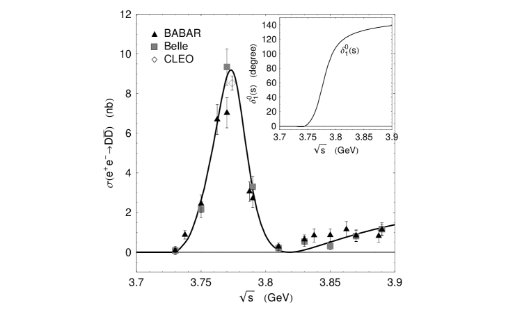
Figure 3: The model of the mixed $\psi^{\prime\prime}$ and $\psi(2S)$ resonances. The curve is the same as the solid curve in Fig. 2, but in comparison only with the data from CLEO Be2 , $BABAR$ Au1 ; Au2 , and Belle Pa Collaborations. The inset shows the phase $\delta^{0}_{1}(s)$ of the form factor $F^{0}_{D}(s)$ and $D\bar{D}$ elastic scattering amplitude $T^{0}_{1}(s)$ for our fit.

Figures 2 and 3 show the fitting of the data Ab3a ; Ab4 ; Be2 ; Au1 ; Au2 ; Pa in the model of the mixed $\psi^{\prime\prime}$ and $\psi(2S)$ resonances. The curves in these figures correspond to the following values of the fitted parameters: $m_{\psi^{\prime\prime}}=3.7884$ GeV, $g_{\psi^{\prime\prime}D\bar{D}}=60.54$,  $g_{\psi^{\prime\prime}\gamma}=-0.2148$ GeV², and $z=1.0225$. Using these values we get $g^{eff}_{\psi^{\prime\prime}D\bar{D}}=14.72$,  $\Gamma_{\psi^{\prime\prime}D\bar{D}}=51.88$ MeV, and $\Gamma_{\psi^{\prime\prime}e^{+}e^{-}}=0.189$ keV. The errors in the values of free parameters do not exceed 5%. For this fit, $\chi^{2}=127.6$, which is approximately 3.6 times less than $\chi^{2}$ for the fit with the solitary $\psi^{\prime\prime}$ resonance shown in Fig. 1. Note that the above value of the width $\Gamma_{\psi^{\prime\prime}D\bar{D}}$ is approximately two times larger than the average value of the total decay width of $\psi^{\prime\prime}$ presented by the PDG. The found mass of $\psi^{\prime\prime}$ is also 15 MeV larger than the average PDG value. However, there is not any contradiction here. The fact is that the parameters of the $\psi^{\prime\prime}$ resonance mixed with the background cannot be directly compared with the PDG values obtained without taking mixing into account. Incidentally, confirmation of the existence of zero in the form factor $F^{0}_{D}(s)$ (see Figs. 2 and 3) would be the best evidence that the observed peak in the region of 3.773 GeV is the result of the interaction between the resonance and background contributions.

The above fit in the model of the mixed $\psi^{\prime\prime}$ and $\psi(2S)$ resonances has been obtained at the fixed value of the parameter $r=12.5$ GeV^-1 ($\approx 2.5$ fm). Let us discuss this parameter in more detail. Its role in the description of the $\psi^{\prime\prime}$ resonance with formulas (1) and (2) was discussed in the second section of Ref. AS12 . Here, a few words about $r$ were said in the two paragraphs after Eq. (16). In Table I, we have collected the conclusions about the parameter $r$ obtained in the processing of the data on the $\psi(3770)$ resonance to illustrate the real situation. The parameter $r$ is practically always taken into account when processing resonance data, but, as a rule, it remains not well-defined and is often simply fixed by hand. Perhaps, its main role is to suppress the increase of the $P$-wave decay width $\psi^{\prime\prime}\to D\bar{D}$ as $\sqrt{s}$ increases, see Eq. (12). The suppression occurs faster at higher $r$. But if the fit improves as $r$ increases, then it simultaneously becomes less sensitive to $g^{2}_{\psi^{\prime\prime}D\bar{D}}$ and $r^{2}$ separately, and increasingly depends on the ratio $g^{2}_{\psi^{\prime\prime}D\bar{D}}/r^{2}$ [see Eq. (12)]. In such a case the parameter $r$ remains formally unbounded from above AS12 . With the sequential increase of $r$, one can estimate its value, after which the $\chi^{2}$ of the fitting actually remains constant. Our fit corresponds to such an approximate value of $r$. If $r$ is decreased, then $\chi^{2}$ will increase, but not catastrophically. For example, $\chi^{2}$ turns out to be $\approx 130.4$ at $r=5$ GeV^-1 ($\approx 1$ fm). In this case $\Gamma_{\psi^{\prime\prime}e^{+}e^{-}}\approx 0.14$ keV, $\Gamma_{\psi^{\prime\prime}D\bar{D}}\approx 92.2$ MeV, and $m_{\psi^{\prime\prime}}\approx 3.796$ GeV. Increasing the data accuracy would make it possible to determine the value of $r$ more accurately and with it the values of other model parameters, too.

Table 1: Information about the parameter $r$ from the $\psi(3770)\to D\bar{D}$ decay descriptions (1 fm $\approx 5$ GeV^-1).

Data processing	Presented conclusions
Rapidis Ra	Acceptable fits for all values of
	$r>1$ fm; illustration at $r=3$ fm
Peruzzi Pe	$r$ was varied from 0 to $\infty$
Schindler Sch	$r$ was taken to be 2.5 fm
Ablikim Ab1	$r$ was taken to be 0.5 fm
Ablikim Ab2	$r$ was left free in the fit
Ablikim Ab3	$r$ was taken to be 1 fm
Ablikim Ab4	$r$ was a free parameter in the fit
Ablikim Ab5	$r$ was fixed at 3 fm
Ablikim Ab6	$r$ was of the order of a few fm
Ablikim Ab7	$r$ was fixed at 1.5 fm
Dobbs Do	$r$ was taken to be 2.4 fm
Anashin An2	$r$ was fixed at 1 fm
Achasov AS12	Analysis of Eqs. (1) and (2) for
	$0<r<4,...$ fm

One can also express the hope that the model will become more flexible and will improve the data description, if at the next step of the research we take into account the couplings of the $\psi^{\prime\prime}$ and $\psi(2S)$ resonances with the closed $D\bar{D}^{*}$ and $D^{*}\bar{D}^{*}$ decay channels in the region $\sqrt{s}$ up to 3.872 GeV and the inelastic effects caused by them for $\sqrt{s}>3.872$ GeV. Of course, further accurate measurements of the $e^{+}e^{-}\to D\bar{D}$ cross sections will be decisive for the selection of phenomenological models and understanding the $\psi(3770)$ resonance as a charm factory.

IV Comparison with theoretical estimates and conclusions

Theoretical estimates of the electronic width of the $\psi^{\prime\prime}$ resonance, that is mainly considered the $1^{3}D_{1}$ charmonium state, show that it is very sensitive to the relativistic corrections, QCD corrections, and mixing of $S-D$ $c\bar{c}$ configurations due to tensor forces and transitions via $D\bar{D}$ coupled-channels Ei75 ; Ei76 ; Ei04 ; Ei80 ; Ei06 ; Ei08 ; No78 ; Ro01 ; Ro05 ; Ja77 ; HTO84 ; So20 ; Bh18 ; Kh18 . The literature cited here presents a rather wide range of theoretical values for $\Gamma_{\psi^{\prime\prime}e^{+}e^{-}}$. For example, in the nonrelativistic limit, $\Gamma_{\psi(3770)e^{+}e^{-}}$ turns out to be $\approx 0.070$ keV due to the $2^{3}S_{1}-1^{3}D_{1}$ mixing in the coupled-channel scheme Ei80 . $\Gamma_{\psi^{\prime\prime}e^{+}e^{-}}$ can increase to $\approx 0.160$ keV Ei80 , if one takes into account the relativistic corrections (i.e., the inequality to zero of the second derivative of the radial wave function at the origin No78 ), and further to $\approx 0.230$ keV with the connection of the the $S-D$ mixing due to tensor forces Ei80 . The relativistic corrections (without mixing) give for $\Gamma_{\psi^{\prime\prime}e^{+}e^{-}}$, for example, $\approx 0.120$ keV No78 or $\approx 0.060$ keV Ro01 . The recent theoretical schemes did not give more definite predictions for the width: $\Gamma_{\psi^{\prime\prime}e^{+}e^{-}}\approx 0.091$ keV So20 , $\approx 0.270$ keV Bh18 , $\approx 0.113$ keV Kh18 .

The spread of theoretical estimates for the width, $\Gamma_{\psi^{\prime\prime}e^{+}e^{-}}$, quite agrees with the spread of its values found in various experiments PDG20 and also in accompanying phenomenological analyses Ya ; LQY ; ZZ ; AS12 ; AS13 ; CZ ; Li ; CL14a ; CL14b ; DMW ; ST ; CG (see discussions in previous sections). Of course, the primary guide is the value of $\Gamma_{\psi^{\prime\prime}e^{+}e^{-}}=(0.262\pm 0.018)$ keV given by the PDG PDG20 . However, as noted above, the phenomenological formulas used to obtain this value were rather simplified (or even poorly grounded). If the errors of the data on $\sigma(e^{+}e^{-}\to D\bar{D})$ are reduced by approximately two times compared to the existing ones [see Figs. (2) and (3)], then it will be possible to abandon such formulas. When processing new, more accurate data on the cross section $\sigma(e^{+}e^{-}\to D^{0}\bar{D}^{0}+D^{+}D^{-})$, it will make sense to take into account the Coulomb interaction in the final state between $D^{+}$ and $D^{-}$ mesons, which amplifies the charged channel by about 8.8% at the peak of the $\psi^{\prime\prime}$ resonance La77 .

Now we summarize: 1) The model of the $D$ meson form factor $F^{0}_{D}(s)$ with good unitary and analytic properties is constructed to describe the cross section of the reaction $e^{+}e^{-}\to D\bar{D}$ near the threshold, 2) The model involves the complex of the mixed $\psi^{\prime\prime}$ and $\psi(2S)$ resonances and satisfactorily describes the data in the $\sqrt{s}$ region up to 3.9 GeV, 3) A feature of the model is the presence of zero in $F^{0}_{D}(s)$ at $\sqrt{s}\approx 3.818$ GeV, 4) The survey of the experimental, phenomenological, and theoretical results for $\Gamma_{\psi^{\prime\prime}e^{+}e^{-}}$ is also presented to illustrate the variety of approaches to determining this quantity, and 5) The rather small value of $\Gamma_{\psi^{\prime\prime}e^{+}e^{-}}\approx 0.19$ keV, obtained by us, and the corresponding value of the ratio $\Gamma_{\psi^{\prime\prime}e^{+}e^{-}}/\Gamma_{\psi(2S)e^{+}e^{-}}\approx 0.081$ indicate in favor of the $D$-wave $c\bar{c}$ nature of the $\psi^{\prime\prime}$ state.

Improving the data on the shape of the $\psi(3770)$ resonance in the $D\bar{D}$ decay channels seems to be an extremely important and quite feasible physical problem.

ACKNOWLEDGMENTS

The work was carried out within the framework of the state contract of the Sobolev Institute of Mathematics, Project No. 0314-2019-0021.

APPENDIX:  THE FUNCTION $h_{\psi^{\prime\prime}}(s)$

The twice subtracted dispersion integral corresponding to the one-loop $P$-wave Feynman diagram has the form:

$$f_{0,+}(s)=\frac{s^{2}}{\pi}\int\limits^{\infty}_{4m^{2}_{D^{0,+}}}\frac{p^{3}_{0,+}(s^{\prime})\,ds^{\prime}}{\sqrt{s^{\prime}}\,s^{\prime 2}(s^{\prime}-s-i\varepsilon)}$$

$$=\frac{s-3m^{2}_{D^{0,+}}}{3\pi}-\frac{s\rho_{0,+}(s)^{3}}{8\pi}\ln\frac{\rho_{0,+}(s)+1}{\rho_{0,+}(s)-1}\,, \mbox{for\ }s<0\,,$$

$$=\frac{s-3m^{2}_{D^{0,+}}}{3\pi}+\frac{s|\rho_{0,+}(s)|^{3}}{8\pi}\left(\pi-2\arctan|\rho_{0,+}(s)|\right), \mbox{for\ }0<s<4m^{2}_{D^{0,+}}\,,$$

$$=\frac{s-3m^{2}_{D^{0,+}}}{3\pi}+\frac{s\rho^{3}_{0,+}(s)}{8\pi}\left(i\pi-\ln\frac{1+\rho_{0,+}(s)}{1-\rho_{0,+}(s)}\right), \mbox{for\ }s>4m^{2}_{D^{0,+}}\,,$$ (A1)

where $\rho_{0,+}(s)=2p_{0,+}(s)/\sqrt{s}=\sqrt{1-4m^{2}_{D^{0,+}}/s}\,$. The polarization operators of the $\psi^{\prime\prime}$ resonance $\Pi^{0}_{\psi^{\prime\prime}}(s)$ and $\Pi^{+}_{\psi^{\prime\prime}}(s)$ corresponding to the contributions of the $D^{0}\bar{D}^{0}$ and $D^{+}D^{-}$ intermediate states are expressed in terms of the functions $f_{0}(s)$ and $f_{+}(s)$ as follows:

$$\Pi^{0,+}_{\psi^{\prime\prime}}(s)=\frac{g^{2}_{\psi^{\prime\prime}D\bar{D}}}{6\pi}\,\frac{s^{2}}{\pi}\int\limits^{\infty}_{4m^{2}_{D^{0,+}}}\frac{p^{3}_{0,+}(s^{\prime})\,ds^{\prime}}{\sqrt{s^{\prime}}\,(1+r^{2}p^{2}_{0,+}(s^{\prime}))\,s^{\prime 2}(s^{\prime}-s-i\varepsilon)}$$

$$=\frac{g^{2}_{\psi^{\prime\prime}D\bar{D}}}{6\pi}\frac{1}{1+r^{2}p^{2}_{0,+}(s)}\left[f_{0,+}(s)-\left(\frac{s}{s_{0,+}}\right)^{2}f_{0,+}(s_{0,+})\right],\quad$$ (A2)

where $s_{0,+}=4(m^{2}_{D^{0,+}}-1/r^{2})$. The knowledge of the $\psi^{\prime\prime}$ mass squared, $m^{2}_{\psi^{\prime\prime}}$, and the $\psi^{\prime\prime}$ width at $s=m^{2}_{\psi^{\prime\prime}}$, $\Gamma_{\psi^{\prime\prime}D\bar{D}}$, allows us to represent the function $h_{\psi^{\prime\prime}}(s)$, entering in Eq. (11), in the form GS ; RP ; BM :

$$h_{\psi^{\prime\prime}}(s)=\mbox{Re}\Pi_{\psi^{\prime\prime}}(s)-\mbox{Re}\Pi_{\psi^{\prime\prime}}(m^{2}_{\psi^{\prime\prime}})-(s-m^{2}_{\psi^{\prime\prime}})\mbox{Re}\Pi^{\prime}_{\psi^{\prime\prime}}(m^{2}_{\psi^{\prime\prime}}),\qquad$$ (A3)

where $\Pi_{\psi^{\prime\prime}}(s)=\Pi^{0}_{\psi^{\prime\prime}}(s)+\Pi^{+}_{\psi^{\prime\prime}}(s)$ is the full polarization operator of $\psi^{\prime\prime}$,

$$\mbox{Im}\Pi_{\psi^{\prime\prime}}(s)=\sqrt{s}\Gamma_{\psi^{\prime\prime}D\bar{D}}(s).$$ (A4)

See Eqs. (11) and (12).

References

- (1) P. A. Zyla et al. (Particle Data Group), Prog. Theor. Exp. Phys. 2020, 083C01 (2020).
- (2) E. Eichten, K. Gottfried, T. Kinoshita, J. B. Kogut, K. D. Lane and T. M. Yan, Phys. Rev. Lett. 34, 369 (1975).
- (3) E. Eichten, K. Gottfried, T. Kinoshita, K. D. Lane and T. M. Yan, Phys. Rev. Lett. 36, 500 (1976).
- (4) J. D. Jackson, in Proceedings of the European Conference on Particle Physics, edited by L. Jenik and I. Montvay (Central Research Institute for Physics, Budapest, 1977), Vol. 1, p. 603.
- (5) V. A. Novikov, L. B. Okun, M. A. Shifman, A. I. Vainshtein, M. B. Voloshin, and V.I. Zakharov, Phys. Rep. 41, 1 (1978).
- (6) E. Eichten, K. Gottfried, T. Kinoshita, K.D. Lane, and T.-M. Yan, Phys. Rev. D 21, 203 (1980).
- (7) K. Heikkillä, N. A. Törnqvist, and Seiji Ono, Phys. Rev. D 29, 110 (1984).
- (8) J. L. Rosner, Phys. Rev. D 64, 094002 (2001).
- (9) E. Eichten, E. J., K. Lane, and C. Quigg, Phys. Rev. D 69, 094019 (2004).
- (10) J. L. Rosner, Ann. Phys. (Amsterdam) 319, 1 (2005).
- (11) E. Eichten, E. J., K. Lane, and C. Quigg, Phys. Rev. D 73, 014014 (2006).
- (12) E. Eichten, S. Godfrey, H. Mahlke, and J. L. Rosner, Rev. Mod. Phys. 80, 1161 (2008).
- (13) P. A. Rapidis et al. (MARK-I Collaboration), Phys. Rev. Lett. 39, 526 (1977).
- (14) I. Peruzzi et al. (MARK-I Collaboration), Phys. Rev. Lett. 39, 1301 (1977).
- (15) W. Bacino et al. (DELCO Collaboration), Phys. Rev. Lett. 40, 671 (1978).
- (16) R. H. Schindler et al. (MARK-II Collaboration), Phys. Rev. D 21, 2716 (1980).
- (17) M. Ablikim et al. (BES Collaboration), Phys. Lett. B 603, 130 (2004).
- (18) M. Ablikim et al. (BES Collaboration), Phys. Rev. Lett. 97, 121801 (2006).
- (19) M. Ablikim et al. (BES Collaboration), Phys. Lett. B 641, 145 (2006).
- (20) M. Ablikim et al. (BES Collaboration), Phys. Rev. Lett. 97, 262001 (2006).
- (21) M. Ablikim et al. (BES Collaboration), Phys. Lett. B 652, 238 (2007).
- (22) M. Ablikim et al. (BES Collaboration), Phys. Lett. B 659, 74 (2008).
- (23) M. Ablikim et al. (BES Collaboration), Phys. Lett. B 660, 315 (2008).
- (24) M. Ablikim et al. (BES Collaboration), Phys. Rev. Lett. 101, 102004 (2008).
- (25) M. Ablikim et al. (BES Collaboration), Phys. Lett. B 668, 263 (2008).
- (26) D. Besson et al. (CLEO Collaboration), Phys. Rev. Lett 96, 092002 (2006).
- (27) S. Dobbs et al. (CLEO Collaboration), Phys. Rev. D 76, 112001 (2007).
- (28) D. Besson et al. (CLEO Collaboration), Phys. Rev. Lett 104, 159901(E) (2010).
- (29) B. Aubert et al. (BABAR Collaboration), Phys. Rev. D 76, 111105(R) (2007); Report No. SLAC-PUB-12818, 2007.
- (30) B. Aubert et al. (BABAR Collaboration), Phys. Rev. D 79, 092001 (2009).
- (31) G. Pakhlova et al. (Belle Collaboration), Phys. Rev. D 77, 011103 (2008).
- (32) V. V. Anashin et al. (KEDR Collaboration), Phys. Lett. B 711, 292 (2012).
- (33) R. Chistov et al. (Belle Collaboration), Phys. Rev. Lett. 93, 051803 (2004).
- (34) J. Brodzicka et al. (Belle Collaboration), Phys. Rev. Lett. 100, 092001 (2008).
- (35) B. Aubert et al. (BABAR Collaboration), Phys. Rev. D 77, 011102 (2008).
- (36) J. P. Less et al. (BABAR Collaboration), Phys. Rev. D 91, 052002 (2015).
- (37) R. Aaij et al., (LHCb Collaboration), Phys. Rev. D 102, 112003 (2020).
- (38) M. Z. Yang, Mod. Phys. Lett. A 23, 3113 (2008).
- (39) H. B. Li, X. S. Qin, and M. Z. Yang, Phys. Rev. D 81, 011501 (2010).
- (40) Y. J. Zhang and Q. Zhao, Phys. Rev. D 81, 034011 (2010).
- (41) N. N. Achasov and G. N. Shestakov, Phys. Rev. D 86, 114013 (2012).
- (42) N. N. Achasov and G. N. Shestakov, Phys. Rev. D 87, 057502 (2013).
- (43) G. Y. Chen and Q. Zhao, Phys. Lett. B 718, 1369 (2013).
- (44) G. Li, X. H. Liu, Q. Wang, and Q. Zhao, (Phys. Rev. D 88, 014010 (2013).
- (45) X. Cao and H. Lenske, Charmonium resonances and Fano line shapes, in Hadron Spectroscopy and Structure (World Sientific, Singapore, 2020), pp. 433–437.
- (46) X. Cao and H. Lenske, arXiv:1410.1375.
- (47) M. L. Du, U.-G. Meissner, and Q. Wang, Phys. Rev. D 94, 096006 (2016).
- (48) A. G. Shamov and K. Yu. Todyshev, Phys. Lett. B 769, 187 (2017).
- (49) S. Coitoa and F. Giacosa, Nucl.Phys. A981, 38 (2019).
- (50) Z. G. He, Y. Fan, and K. T. Chao, Phys. Rev. Lett. 101, 112001 (2008).
- (51) Z. G. He, Y. Fan, and K. T. Chao, Phys. Rev. D 81, 074032 (2010).
- (52) K. M. Watson, Phys. Rev. 88, 1163 (1952).
- (53) J. M. Blatt and V. F. Weisskopf, Theoretical Nuclear Physics (Wiley, New York, 1952).
- (54) A. D. Bukin, arXiv:0710.5627.
- (55) K. Zhu, X. H. Mo, C. Z. Yuan, and P. Wang, Int.J. Mod. Phys. A 26, 4511 (2011).
- (56) C. Z. Yuan, Chin. Phys. C 38, 043001 (2014).
- (57) Important examples of the form factors described by solitary resonances were constructed in the works GS ; RP ; BM .
- (58) G. J. Gounaris and J.J. Sakurai, Phys. Rev. Lett. 21, 244 (1968).
- (59) M. Roos and J. Pišút, Nucl. Phys. B10, 563 (1969).
- (60) G. Bonneau and F. Martin, Nuovo Cimento A 13, 413 (1973).
- (61) The possible position of zero in is consistent with the prediction of the coupled-channel model Ei80 .
- (62) N. R. Soni, R. M. Parekh, J. J. Patel, A. N. Gadaria, and J. N. Pandya, arXiv:2012.00294.
- (63) T. Bhavsar, M. Shah, and P. C. Vinodkumar, Eur. Phys. J. C 78, 227 (2018).
- (64) V. Kher and A. K. Rai, Chin. Phys. C 42, 083101 (2018).
- (65) L. D. Landau and E. M. Lifshits, Quantum Mechanics (Non-Relativistic Theory), 3rd ed. (Pergamon, Oxford, 1977).