Mesh-robustness of an energy stable BDF2 scheme with
variable steps for the Cahn-Hilliard model

Abstract

The two-step backward differential formula (BDF2) with unequal time-steps is applied to construct an energy stable convex-splitting scheme for the Cahn-Hilliard model. We focus on the numerical influences of time-step variations by using the recent theoretical framework with the discrete orthogonal convolution kernels. Some novel discrete convolution embedding inequalities with respect to the orthogonal convolution kernels are developed such that a concise $L^{2}$ norm error estimate is established at the first time under an updated step-ratio restriction $0<r_{k}:=\tau_{k}/\tau_{k-1}\leq r_{\mathrm{user}}$, where $r_{\mathrm{user}}$ can be chosen by the user such that $r_{\mathrm{user}}<4.864$. The stabilized convex-splitting BDF2 scheme is shown to be mesh-robustly convergent in the sense that the convergence constant (prefactor) in the error estimate is independent of the adjoint time-step ratios. The suggested method is proved to preserve a modified energy dissipation law at the discrete levels if $0<r_{k}\leq r_{\mathrm{user}}$, such that it is mesh-robustly stable in an energy norm. On the basis of ample tests on random time meshes, a useful adaptive time-stepping strategy is applied to efficiently capture the multi-scale behaviors and to accelerate the long-time simulation approaching the steady state.
Keywords:   Cahn-Hilliard model; adaptive BDF2 method; discrete energy dissipation law; orthogonal convolution kernels; discrete convolution embedding inequality; error estimate
AMS subject classifications.   35Q99, 65M06, 65M12, 74A50

1 Introduction

The Cahn-Hilliard (CH) model is an efficient approach to describe the coarsening dynamics of a binary alloy system [4] and has been applied in other fields including image inpainting [2] and tumor growth [5]. Consider a free energy functional of Ginzburg–Landau type,

$$E[\Phi]=\int_{\Omega}\Big{[}\frac{\epsilon^{2}}{2}|\nabla\Phi|^{2}+F(\Phi)\Big{]}\,\mathrm{d}\boldsymbol{x}\quad\text{with}\quad F(\Phi):=\frac{1}{4}(\Phi^{2}-1)^{2}$$ (1.1)

where $\boldsymbol{x}\in\Omega\subseteq\mathbb{R}^{2}$ and $0<\epsilon<1$ is a bounded parameter that is proportional to the interface width. Then the Cahn-Hilliard equation would be given by the $H^{-1}$ gradient flow associated with the free energy functional $E[\Phi]$,

$$\partial_{t}\Phi=\kappa\Delta\mu\quad\text{with}\quad\mu:=\tfrac{\delta E}{\delta\Phi}=F^{\prime}(\Phi)-\epsilon^{2}\Delta\Phi,$$ (1.2)

where the parameter $\kappa$ is the mobility related to the characteristic relaxation time of system and $\mu$ is the chemical potential. Assume that $\Phi$ is periodic over the domain $\Omega$. By applying the integration by parts, one can find the volume conservation,

$$\big{(}\Phi(t),1\big{)}=\big{(}\Phi(t_{0}),1\big{)},$$ (1.3)

and the following energy dissipation law,

$$\frac{\,\mathrm{d}{E}}{\,\mathrm{d}{t}}=\big{(}\tfrac{\delta E}{\delta\Phi},\partial_{t}\Phi\big{)}=\kappa\left(\mu,\Delta\mu\right)=-\kappa\left\|\nabla\mu\right\|^{2}\leq 0,$$ (1.4)

where $\left(u,v\right):=\int_{\Omega}uv\,\mathrm{d}{\boldsymbol{x}}$, and the associated $L^{2}$ norm $\left\|v\right\|=\sqrt{\left(v,v\right)}$ for all $u,v\in{L}^{2}(\Omega)$.

The main aim of this paper is to present a rigorous stability and convergence analysis of the BDF2 method with variable time-steps for simulating the CH model (1.2). Consider the nonuniform time levels $0=t_{0}<t_{1}<\cdots<t_{N}=T$ with the time-step sizes $\tau_{k}:=t_{k}-t_{k-1}$ for $1\leq k\leq N$, and denote the maximum time-step size $\tau:=\max_{1\leq k\leq N}\tau_{k}$. Let the adjoint time-step ratio $r_{k}:=\tau_{k}/\tau_{k-1}$ for $2\leq k\leq N$. Our analysis will focus on the influence of non-uniform time grids (with the associated time-step ratios) on the numerical solution by carefully evaluating the stability and convergence.

This is motivated by the following facts:

• The BDF2 method is A-stable and L-stable such that it would be more suitable than Crank-Nicolson type schemes for solving the stiff dissipative problems, see e.g. [3, 6].

• The nonuniform grid and adaptive time-stepping techniques [12, 18, 19, 20, 24] are powerful in capturing the multi-scale behaviors and accelerating the long-time simulations of phase field models including the CH model.

• The convergence theory of variable-steps BDF2 scheme remains incomplete for nonlinear parabolic equations. Actually, the required step-ratio constraint for the $L^{2}$ norm stability are severer than the classical zero-stability condition $r_{k}<1+\sqrt{2}$, given by Grigorieff [11]. Always, they contain some undesirable pre-factors $C_{r}\exp(C_{r}\Gamma_{n})$ or $C_{r}\exp(C_{r}t_{n})$, see e.g. [1, 9, 10, 28], where $\Gamma_{n}$ may be unbounded when certain time-step variations appear and $C_{r}$ may be infinity as the step-ratios approach the zero-stability limit $1+\sqrt{2}$.

In recent works [18, 19, 22], a novel technique with discrete orthogonal convolution (DOC) kernels was suggested to verify that, if $0<r_{k}<\left(3+\sqrt{17}\right)/2\approx 3.561$, the BDF2 scheme is computationally robust with respect to the time-step variations for linear diffusions [22], the phase field crystal model [18] and the molecular beam epitaxial model without slope selection [19].

Nonetheless, due to the lack of some convolution embedding inequalities with respect to the DOC kernels, the techniques in [18, 19, 22] are inadequate to handle more general nonlinear problems such as the underlying nonlinear CH model (and Allen-Chan model). The main aim of this paper is to fill this gap by establishing some discrete convolution embedding inequalities with respect to the DOC kernels. Also, the recent analysis in [18, Lemma A.1] with a step-scaled matrix motivates us to update the previous zero-stability restriction in [22] as follows,

1. $0<r_{k}\leq r_{\mathrm{user}}(<4.864)$  for  $2\leq k\leq N$,

where the value of $r_{\mathrm{user}}$ can be chosen in adaptive time-stepping computations by the user such that $r_{\mathrm{user}}<4.864$, such as $r_{\mathrm{user}}=2,3$ or 4 for practical choices. Under the step-ratio constraint $\mathbf{S0}$, we will present an $L^{2}$ norm error estimate with an improved prefactor, see Theorem 4.1,

$$C_{\phi}\exp\big{(}c_{\epsilon}t_{n-1}\big{)}.$$

Here and hereafter, any subscripted $C$, such as $C_{u}$ and $C_{\phi}$, denotes a generic positive constant, not necessarily the same at different occurrences; while, any subscripted $c$, such as $c_{\epsilon},c_{\Omega},c_{p},c_{z}$ and so on, denotes a fixed constant. The appeared constants may be dependent on the given data (typically, the interface width parameter $\epsilon$) and the solution but are always independent of the spatial lengths, the time $t_{n}$, the step sizes $\tau_{n}$ and the step ratios $r_{n}$. It is interesting to emphasize that, under the step-ratio constraint $\mathbf{S0}$, the involved constants are bounded even when the step-ratios $r_{n}$ approach $r_{\mathrm{user}}$ such that the BDF2 scheme is mesh-robustly convergent.

To the best of our knowledge, this is the first time such an optimal $L^{2}$ norm error estimate of variable-steps BDF2 method is established for the Cahn-Hiliard (and Allen-Cahn) type models. As a closely related work, the BDF2 scheme for the Allen-Chan equation was also investigated in [20] by using the discrete complementary convolution kernels. The BDF2 scheme was proved to preserve the maximum bound principle if the step-ratios satisfy the classical zero-stability condition $r_{k}<1+\sqrt{2}$. The maximum norm error estimate with a prefactor $\frac{1}{1-\eta}\exp(\frac{t_{n}}{1-\eta})$ was obtained, where the parameter $\eta\rightarrow 1$ as $\max r_{k}\rightarrow 1+\sqrt{2}$. It is to mention that, under the constraint $\mathbf{S0}$, one can follow the present analysis to obtain a new $L^{2}$ norm error estimate that is robustly stable to the variations of time-steps.

Given a grid function $\{v^{k}\}_{k=0}^{N}$, put $\triangledown_{\tau}v^{k}:=v^{k}-v^{k-1}$, $\partial_{\tau}v^{k}:=\triangledown_{\tau}v^{k}/\tau_{k}$ for $k\geq{1}$. Taking $v^{n}=v(t_{n})$, we view the variable-steps BDF2 formula as a discrete convolution summation

$$D_{2}v^{n}:=\sum_{k=1}^{n}b_{n-k}^{(n)}\triangledown_{\tau}v^{k}\quad\text{for $n\geq 2$},$$ (1.5)

where the discrete convolution kernels $b_{n-k}^{(n)}$ are defined for $n\geq 2$,

$$b_{0}^{(n)}:=\frac{1+2r_{n}}{\tau_{n}(1+r_{n})},\quad b_{1}^{(n)}:=-\frac{r_{n}^{2}}{\tau_{n}(1+r_{n})}\quad\text{and}\quad b_{j}^{(n)}:=0\quad\mathrm{for}\quad j\geq 2.$$ (1.6)

Without losing the generality, assume that an accurate solution $\phi^{1}$ is available. We consider the stability and convergence of the convex-splitting BDF2 scheme for solving the CH equation (1.2) subject to the periodic boundary conditions:

$$D_{2}\phi^{n}=\kappa\Delta_{h}\mu^{n}\quad\text{with}\quad\mu^{n}:=\big{(}\phi^{n}\big{)}^{3}-\hat{\phi}^{n}-\left(\epsilon^{2}+A\tau^{2}\right)\Delta_{h}\phi^{n}\quad\text{for $2\leq n\leq N$},$$ (1.7)

where $\hat{\phi}^{n}:=\left(1+r_{n}\right)\phi^{n-1}-r_{n}\phi^{n-2}$ and the stabilized parameter $A>0$. The spatial operators are approximated by the Fourier pseudo-spectral method, as described in the next section.

The unique solvability of the convex-splitting scheme (1.7) is established in Theorem 2.1 by using the fact that the solution of nonlinear scheme (1.7) is equivalent to the minimization of a convex functional. Lemma 2.1 shows that the BDF2 convolution kernels $b_{n-k}^{(n)}$ are positive definite provided the adjacent time-step rations $r_{k}$ satisfy $\mathbf{S0}$. Theorem 2.2 shows that the convex-splitting BDF2 method (1.7) has a modified energy dissipation law at the discrete levels for a properly large parameter $A$, see Remark 3.

We are to emphasize that the solution estimates in section 2 are based on the original form (1.7), but in the subsequent $L^{2}$ norm error analysis we will use an equivalent convolution form with a class of discrete orthogonal convolution (DOC) kernels. The DOC kernels $\{\theta_{n-k}^{(n)}\}_{k=2}^{n}$ are defined by (this definition is slightly different from those in [18, 19, 22] since we do not introduce the discrete kernel $b_{0}^{(1)}$ for the first-level solver)

$$\theta_{0}^{(n)}:=\frac{1}{b_{0}^{(n)}}\;\;\text{for $n\geq 2$}\quad\mathrm{and}\quad\theta_{n-k}^{(n)}:=-\frac{1}{b_{0}^{(k)}}\sum_{j=k+1}^{n}\theta_{n-j}^{(n)}b_{j-k}^{(j)}\quad\text{for $n\geq k+1\geq 3$}.$$ (1.8)

One has the following discrete orthogonal identity

$$\sum_{j=k}^{n}\theta_{n-j}^{(n)}b_{j-k}^{(j)}\equiv\delta_{nk}\quad\text{for $2\leq k\leq n$,}$$ (1.9)

where $\delta_{nk}$ is the Kronecker delta symbol. By exchanging the summation order and using the identity (1.9), it is not difficult to check that

$$\sum_{j=2}^{n}\theta_{n-j}^{(n)}D_{2}v^{j}= \,\sum_{j=2}^{n}\theta_{n-j}^{(n)}b_{j-1}^{(j)}\triangledown_{\tau}v^{1}+\sum_{j=2}^{n}\theta_{n-j}^{(n)}\sum_{\ell=2}^{j}b_{j-\ell}^{(j)}\triangledown_{\tau}v^{\ell}$$

$$= \,\theta_{n-2}^{(n)}b_{1}^{(2)}\triangledown_{\tau}v^{1}+\triangledown_{\tau}v^{n}\quad\text{for $n\geq 2$.}$$ (1.10)

Acting the DOC kernels $\theta_{m-n}^{(m)}$ on the first equation in (1.7) and summing $n$ from $n=2$ to $m$, we apply (1) to find the equivalent convolution form (replacing $m$ by $n$)

$$\triangledown_{\tau}\phi^{n}=-\theta_{n-2}^{(n)}b_{1}^{(2)}\triangledown_{\tau}\phi^{1}+\kappa\sum_{j=2}^{n}\theta_{n-j}^{(n)}\Delta_{h}\mu^{j}\quad\text{for $2\leq n\leq N$.}$$ (1.11)

Note that, by following the proof of [21, Lemma 2.1], we have

$$\sum_{j=k}^{m}b_{m-j}^{(m)}\theta_{j-k}^{(j)}\equiv\delta_{mk}\quad\text{for $2\leq k\leq m$.}$$ (1.12)

With the help of this mutually orthogonal identity, one can recover the original form (1.7) by acting the BDF2 kernels $b_{m-n}^{(m)}$ on the new formulation (1.11). In this sense, the DOC kernels define a reversible discrete transform between (1.7) and the convolution form (1.11).

To perform the $L^{2}$ norm error analysis, section 3 presents some properties of the DOC kernels $\theta_{n-k}^{(n)}$ and some new convolution embedding inequalities with respect to the DOC kernels, see Lemmas 3.1–3.9. By making use of the $H^{1}$ norm solution bound obtained in Lemma 2.2, we establish an optimal $L^{2}$ norm error estimate in section 4. Numerical tests and comparisons are presented in section 5 to validate the accuracy and effectiveness of the BDF2 method (1.7), especially when coupled with an adaptive stepping strategy.

2 Solvability and energy dissipation law

We use the same spatial notations in [18]. Set the space domain $\Omega=(0,L)^{2}$ and consider the uniform length $h_{x}=h_{y}=h:=L/M$ in each direction for an even positive integer $M$. Let $\Omega_{h}:=\big{\{}\boldsymbol{x}_{h}=(ih,jh)\,|\,1\leq i,j\leq M\big{\}}$ and put $\bar{\Omega}_{h}:=\Omega_{h}\cup\partial{\Omega}$. Denote the space of $L$-periodic grid functions $\mathbb{V}_{h}:=\{v\,|\,v=\left(v_{h}\right)\;\text{is $L$-periodic for}\;\boldsymbol{x}_{h}\in\bar{\Omega}_{h}\}.$

For a periodic function $v(\boldsymbol{x})$ on $\bar{\Omega}$, let $P_{M}:L^{2}(\Omega)\rightarrow\mathscr{F}_{M}$ be the standard $L^{2}$ projection operator onto the space $\mathscr{F}_{M}$, consisting of all trigonometric polynomials of degree up to $M/2$, and $I_{M}:L^{2}(\Omega)\rightarrow\mathscr{F}_{M}$ be the trigonometric interpolation operator [25], i.e.,

$$\left(P_{M}v\right)(\boldsymbol{x})=\sum_{\ell,m=-M/2}^{M/2-1}\widehat{v}_{\ell,m}e_{\ell,m}(\boldsymbol{x}),\quad\left(I_{M}v\right)(\boldsymbol{x})=\sum_{\ell,m=-M/2}^{M/2-1}\widetilde{v}_{\ell,m}e_{\ell,m}(\boldsymbol{x}),$$

where the complex exponential basis function $e_{\ell,m}(\boldsymbol{x}):=e^{\mathrm{i}\nu\left(\ell x+my\right)}$ with $\nu=2\pi/L$. The coefficients $\widehat{v}_{\ell,m}$ refer to the standard Fourier coefficients of function $v(\boldsymbol{x})$, and the pseudo-spectral coefficients $\widetilde{v}_{\ell,m}$ are determined such that $\left(I_{M}v\right)(\boldsymbol{x}_{h})=v_{h}$.

The Fourier pseudo-spectral first and second order derivatives of $v_{h}$ are given by

$$\mathcal{D}_{x}v_{h}:=\sum_{\ell,m=-M/2}^{M/2-1}\left(\mathrm{i}\nu\ell\right)\widetilde{v}_{\ell,m}e_{\ell,m}(\boldsymbol{x}_{h}),\quad\mathcal{D}_{x}^{2}v_{h}:=\sum_{\ell,m=-M/2}^{M/2-1}\left(\mathrm{i}\nu\ell\right)^{2}\widetilde{v}_{\ell,m}e_{\ell,m}(\boldsymbol{x}_{h}).$$

The differentiation operators $\mathcal{D}_{y}$ and $\mathcal{D}_{y}^{2}$ can be defined in the similar fashion. In turn, we can define the discrete gradient and Laplacian in the point-wise sense, respectively, by

$$\nabla_{h}v_{h}:=\left(\mathcal{D}_{x}v_{h},\mathcal{D}_{y}v_{h}\right)^{T}\quad\text{and}\quad\Delta_{h}v_{h}:=\left(\mathcal{D}_{x}^{2}+\mathcal{D}_{y}^{2}\right)v_{h}.$$

For any grid functions $v,w\in\mathbb{V}_{h}$, define the discrete inner product $\left\langle v,w\right\rangle:=h^{2}\sum_{\boldsymbol{x}_{h}\in\Omega_{h}}v_{h}w_{h}$, and the associated $L^{2}$ norm $\left\|v\right\|:=\left\|v\right\|_{l^{2}}=\sqrt{\left\langle v,v\right\rangle}$. Also, we will use the discrete $l^{q}$ norm $\left\|v\right\|_{l^{q}}:=\sqrt[q]{h^{2}\sum_{\boldsymbol{x}_{h}\in\Omega_{h}}|v_{h}|^{q}}$ and the $H^{1}$ seminorm $\big{\|}\nabla_{h}v\big{\|}:=\sqrt{h^{2}\sum_{\boldsymbol{x}_{h}\in\Omega_{h}}|\nabla_{h}v_{h}|^{2}}$. It is easy to check the discrete Green’s formulas, $\left\langle-\Delta_{h}v,w\right\rangle=\left\langle\nabla_{h}v,\nabla_{h}w\right\rangle$ and $\left\langle\Delta_{h}^{2}v,w\right\rangle=\left\langle\Delta_{h}v,\Delta_{h}w\right\rangle$, see [25, 7, 6] for more details. Also we have the following discrete embedding inequality simulating the Sobolev embedding $H^{1}(\Omega)\hookrightarrow L^{6}(\Omega)$,

$$\big{\|}v\big{\|}_{l^{6}}\leq c_{\Omega}\big{(}\big{\|}v\big{\|}+\big{\|}\nabla_{h}v\big{\|}\big{)}\quad\text{for any $v\in\mathbb{V}_{h}$.}$$ (2.1)

For the underlying volume-conservative problem, it is also to define a mean-zero function space $\mathbb{\mathring{V}}_{h}:=\big{\{}v\in\mathbb{V}_{h}\,|\,\left\langle v,1\right\rangle=0\big{\}}\subset\mathbb{V}_{h}.$ As usual, following the arguments in [8, 6], one can introduce an discrete version of inverse Laplacian operator $\left(-\Delta_{h}\right)^{-\gamma}$ as follows. For a grid function $v\in\mathbb{\mathring{V}}_{h}$, define

$$\left(-\Delta_{h}\right)^{-\gamma}v_{h}:=\sum_{\mbox{\tiny$\begin{array}[]{c}\ell,m=-M/2\\ \left(\ell,m\right)\neq\mathbf{0}\end{array}$}}^{M/2-1}\left(\nu^{2}\left(\ell^{2}+m^{2}\right)\right)^{-\gamma}\widetilde{v}_{\ell,m}e_{\ell,m}(\boldsymbol{x}_{h}),$$

and an $H^{-1}$ inner product $\left\langle v,w\right\rangle_{-1}:=\big{\langle}\left(-\Delta_{h}\right)^{-1}v,w\big{\rangle}.$ The associated $H^{-1}$ norm $\left\|\cdot\right\|_{-1}$ can be defined by $\left\|v\right\|_{-1}:=\sqrt{\left\langle v,v\right\rangle_{-1}}\,.$ We have the following Poincaré type inequality with the usual Poincaré constant $c_{p}$, $\big{\|}v\big{\|}_{-1}\leq c_{p}\big{\|}v\big{\|}$, and the generalized Hölder inequality,

$$\big{\|}v\big{\|}^{2}\leq\big{\|}\nabla_{h}v\big{\|}\big{\|}v\big{\|}_{-1}\quad\text{for any $v\in\mathbb{\mathring{V}}_{h}$.}$$ (2.2)

Also the discrete embedding inequality (2.1) can be simplified as ($c_{z}:=c_{\Omega}+c_{\Omega}c_{p}$)

$$\big{\|}v\big{\|}_{l^{6}}\leq c_{z}\big{\|}\nabla_{h}v\big{\|}\quad\text{for any $v\in\mathbb{\mathring{V}}_{h}$.}$$ (2.3)

2.1 Unique solvability

Let $E[\phi^{k}]$ be the discrete version of free energy functional (1.1), given by

$$E[\phi^{k}]:=\frac{\epsilon^{2}}{2}\big{\|}\nabla_{h}\phi^{k}\big{\|}^{2}+\big{\langle}F(\phi^{k}),1\big{\rangle}\quad\text{for $k\geq 1$.}$$ (2.4)

To focus on the numerical analysis of the BDF2 solution, it is to assume that

1. A starting scheme is properly chosen to compute the first-level solution $\phi^{1}$ such that it preserves the volume, $\big{\langle}\phi^{1},1\big{\rangle}=\big{\langle}\phi^{0},1\big{\rangle}=\big{\langle}P_{M}\Phi^{0},1\big{\rangle}$, and also preserves certain (maybe, modified) energy dissipation law. There exists a positive constant $c_{0}$, depended on the domain $\Omega$, the mobility $\kappa$, the interface parameter $\epsilon$ and the initial value $\phi^{0}$, such that

   $$E[\phi^{1}]+\frac{\tau_{2}}{2\kappa}\big{\|}\partial_{\tau}\phi^{1}\big{\|}_{-1}^{2}+\frac{\tau_{1}\tau_{2}}{2}\big{\|}\partial_{\tau}\phi^{1}\big{\|}^{2}+\frac{A\tau^{2}}{2}\big{\|}\nabla_{h}\phi^{1}\big{\|}^{2}\leq c_{0}.$$

Remark 1.

Assumption $\mathbf{A1}$ can be satisfied by many of first-level solvers. The BDF1 scheme would be suited for computing a second-order solution $\phi^{1}$; however, a very small initial step $\tau_{1}$ would not be suggested here since it arrives at a large step-ratio $r_{2}$ and eventually affects the accuracy of solution in the whole simulation, see numerical results in [23].

The Crank-Nicolson scheme at the first time-level can generate a second-order difference quotient $\partial_{\tau}\phi^{1}$; but a very small initial step $\tau_{1}$ would not be suggested either because it would be prone to generate nonphysical oscillations. To control possibly initial oscillations, we suggest a special step-ratio $r_{2}=\sqrt{2}/2$ in the implementation of our scheme (1.7). Actually, by taking $\phi^{\gamma}:=\phi^{1}$, $\phi^{1}:=\phi^{2}$, $\tau_{*}:=\tau_{1}+\tau_{2}$ and $\gamma:=\tau_{1}/\tau_{*}$ with $r_{2}=1/\gamma-1$ , the first two steps of (1.7) are equivalent to the following TR-BDF2 method

$$\frac{\phi^{\gamma}-\phi^{0}}{\gamma\tau_{*}}= \,\frac{\kappa}{2}\Delta_{h}\mu^{\gamma}+\frac{\kappa}{2}\Delta_{h}\mu^{0},\quad\frac{2-\gamma}{(1-\gamma)\tau_{*}}\phi^{1}-\frac{1}{\gamma(1-\gamma)\tau_{*}}\phi^{\gamma}+\frac{1-\gamma}{\gamma\tau_{*}}\phi^{0}=\kappa\Delta_{h}\mu^{1},$$

which was shown to be L-stable for $\gamma=2-\sqrt{2}$, see [16, 27].

Under the assumption $\mathbf{A1}$, the solution $\phi^{n}$ of the BDF2 scheme (1.7) preserves the volume, $\big{\langle}\phi^{n},1\big{\rangle}=\big{\langle}\phi^{0},1\big{\rangle}$ for $n\geq 2$. Actually, taking the inner product of (1.7) by 1 and applying the discrete Green’s formulas, one can check that $\big{\langle}D_{2}\phi^{j},1\big{\rangle}=0$ for $j\geq 2$. Multiplying both sides of this equality by the DOC kernels $\theta_{n-j}^{(n)}$ and summing the index $j$ from $j=2$ to $n$, we get

$$\sum_{j=2}^{n}\theta_{n-j}^{(n)}\big{\langle}D_{2}\phi^{j},1\big{\rangle}=0\quad\text{for $n\geq 2$}.$$

It leads to $\big{\langle}\triangledown_{\tau}\phi^{n},1\big{\rangle}=0$ directly by taking $v^{j}=\phi^{j}$ in the equality (1). Simple induction yields the volume conversation law, $\big{\langle}\phi^{n},1\big{\rangle}=\big{\langle}\phi^{n-1},1\big{\rangle}=\cdots=\big{\langle}\phi^{0},1\big{\rangle}$ for $n\geq 1$.

Theorem 2.1.

If $\mathbf{A1}$ holds, the convex-splitting BDF2 scheme (1.7) is uniquely solvable.

Proof.

For any fixed time-level indexes $n\geq 2$, consider the following energy functional $G$ on the space $\mathbb{V}_{h}^{*}:=\big{\{}z\in\mathbb{V}_{h}\,|\,\big{\langle}z,1\big{\rangle}=\big{\langle}\phi^{n-1},1\big{\rangle}\big{\}},$

$$G[z]:= \frac{b_{0}^{(n)}}{2}\big{\|}z-\phi^{n-1}\big{\|}_{-1}^{2}+b_{1}^{(n)}\big{\langle}\triangledown_{\tau}\phi^{n-1},z-\phi^{n-1}\big{\rangle}_{-1}$$

$$\quad+\frac{\kappa}{2}\big{(}\epsilon^{2}+A\tau^{2}\big{)}\big{\|}\nabla_{h}z\big{\|}^{2}+\kappa\big{\langle}z^{3}/4-\hat{\phi}^{n},z\big{\rangle}.$$ (2.5)

It is easily to verity the functional $G$ is strictly convex since, for any $\lambda\in\mathbb{R}$ and any $\psi\in\mathbb{\mathring{V}}_{h}$,

$$\frac{\,\mathrm{d}^{2}G}{\,\mathrm{d}\lambda^{2}}[z+\lambda\psi]\Big{|}_{\lambda=0}= \,b_{0}^{(n)}\big{\|}\psi\big{\|}_{-1}^{2}+\kappa\big{(}\epsilon^{2}+A\tau^{2}\big{)}\big{\|}\nabla_{h}\psi\big{\|}^{2}+3\kappa\big{\|}z\psi\big{\|}^{2}>0.$$

Thus the functional $G$ has a unique minimizer, denoted by $\phi^{n}$, if and only if it solves the equation

$$0=\frac{\,\mathrm{d}G}{\,\mathrm{d}\lambda}[z+\lambda\psi]\Big{|}_{\lambda=0}= \,\big{\langle}b_{0}^{(n)}(z-\phi^{n-1})+b_{1}^{(n)}\triangledown_{\tau}\phi^{n-1},\psi\big{\rangle}_{-1}+\kappa\big{\langle}z^{3}-\hat{\phi}^{n}-\big{(}\epsilon^{2}+A\tau^{2}\big{)}\Delta_{h}z,\psi\big{\rangle}$$

$$= \,\Big{\langle}b_{0}^{(n)}(z-\phi^{n-1})+b_{1}^{(n)}\triangledown_{\tau}\phi^{n-1}-\kappa\Delta_{h}\big{[}z^{3}-\hat{\phi}^{n}-\big{(}\epsilon^{2}+A\tau^{2}\big{)}\Delta_{h}z\big{]},\psi\Big{\rangle}_{-1}.$$

This equation holds for any $\psi\in\mathbb{\mathring{V}}_{h}$ if and only if the unique minimizer $\phi^{n}\in\mathbb{V}_{h}^{*}$ solves

$$b_{0}^{(n)}(\phi^{n}-\phi^{n-1})+b_{1}^{(n)}\triangledown_{\tau}\phi^{n-1}-\kappa\Delta_{h}\big{[}(\phi^{n})^{3}-\hat{\phi}^{n}-\big{(}\epsilon^{2}+A\tau^{2}\big{)}\Delta_{h}\phi^{n}\big{]}=0,$$

which is just the convex-splitting BDF2 scheme (1.7). It completes the proof. ∎

2.2 Discrete energy dissipation law

In our previous work [22, Lemma 2.1], the BDF2 kernels $b_{n-k}^{(n)}$ are shown to be positive definite if the adjacent time-step ratios $0<r_{k}<\frac{3+\sqrt{17}}{2}$. The following result shows that this sufficient condition can be further improved in the theoretical manner. This improvement is inspired by [18, LemmaA.1] to find a lower bound for the eigenvalues of the step-scaled matrix $\widetilde{B}$, see Lemma 3.2 below. For simplicity, we denote

$$R_{L}\left(z,s\right):=\frac{2+4z-z^{3/2}}{1+z}-\frac{s^{3/2}}{1+s},\quad\text{for $0<z,s<r_{*},$}$$ (2.6)

where $r_{*}\approx 4.864$ is the positive root of the equation $1+2r_{*}-r_{*}^{3/2}=0$. According to the proof of [18, LemmaA.1], $R_{L}\big{(}z,s\big{)}$ is increasing in $(0,1)$ and decreasing in $(1,r_{*})$ with respect to $z$. Also, $R_{L}\left(z,s\right)$ is decreasing with respect to $s$ such that

$$R_{L}\left(z,s\right)>\min\{R_{L}\left(0,r_{*}\right),R_{L}\big{(}r_{*},r_{*}\big{)}\}=\frac{2(1+2r_{*}-r_{*}^{3/2})}{1+z}=0\quad\text{for $0<z,s<r_{*}$}.$$

Lemma 2.1.

Let $0<r_{k}<4.864$ for $2\leq k\leq N$. For any real sequence $\{w_{k}\}_{k=1}^{n}$, it holds that

$$2w_{k}\sum_{j=1}^{k}b_{k-j}^{(k)}w_{j}\geq\frac{r_{k+1}^{3/2}}{1+r_{k+1}}\frac{w_{k}^{2}}{\tau_{k}}-\frac{r_{k}^{3/2}}{1+r_{k}}\frac{w_{k-1}^{2}}{\tau_{k-1}}+R_{L}(r_{k},r_{k+1})\frac{w_{k}^{2}}{\tau_{k}}\quad\text{for $k\geq 2$}.$$

So the discrete convolution kernels $b_{k-j}^{(k)}$ are positive definite in the sense that

$$2\sum_{k=2}^{n}w_{k}\sum_{j=2}^{k}b_{k-j}^{(k)}w_{j}\geq\sum_{k=2}^{n}R_{L}(r_{k},r_{k+1})\frac{w_{k}^{2}}{\tau_{k}}\quad\text{for $n\geq 2$}.$$

Proof.

Applying the inequality $-2ab\geq-a^{2}-b^{2}$, we take $u_{k}:=w_{k}/\sqrt{\tau_{k}}$ to find

$$2w_{k}\sum_{j=1}^{k}\frac{1}{\tau_{k}^{2}}b_{k-j}^{(k)}w_{j} =2\tau_{k}b_{0}^{(k)}u_{k}^{2}+2\sqrt{\tau_{k}\tau_{k-1}}b_{1}^{(k)}u_{k}u_{k-1}$$

$$\geq\frac{2+4r_{k}}{1+r_{k}}u_{k}^{2}-\frac{r_{k}^{3/2}}{1+r_{k}}\left(u_{k}^{2}+u_{k-1}^{2}\right)$$

$$=\frac{r_{k+1}^{3/2}}{1+r_{k+1}}\frac{w_{k}^{2}}{\tau_{k}}-\frac{r_{k}^{3/2}}{1+r_{k}}\frac{w_{k-1}^{2}}{\tau_{k-1}}+R_{L}(r_{k},r_{k+1})\frac{w_{k}^{2}}{\tau_{k}}\quad\text{for $k\geq 2$.}$$

Summing this inequality from $k=2$ to $n$, it is straightforward to obtain the claimed positive definiteness result. It completes the proof. ∎

Remark 2.

This lemma updates the sufficient condition of [22, Lemma 2.1]. Thus by following the discussions in [22, Remark 3 and Remark 5], one can verify that the variable-step BDF2 method is A-stable if $0<r_{k}<4.864$ for $2\leq k\leq N$.

Next theorem shows that the numerical scheme (1.7) preserves a modified energy dissipation property at the discrete levels, and it is mesh-robustly stable in an energy norm.

Theorem 2.2.

Let $\mathbf{S0}$ holds. If the stabilized parameter $A$ is properly large such that

$$A\geq\frac{(r_{n}+r_{n+1}-1)^{4}}{64R_{L}^{2}(r_{n},r_{n+1})}\frac{\kappa^{2}}{\epsilon^{2}},$$ (2.7)

the convex-splitting BDF2 scheme (1.7) preserves the following energy dissipation law

$$\mathcal{E}[\phi^{n}]\leq\mathcal{E}[\phi^{n-1}]\leq\mathcal{E}[\phi^{1}]\quad\text{for $n\geq 2$,}$$

where the modified discrete energy $\mathcal{E}[\phi^{k}]$ is defined by

$$\mathcal{E}[\phi^{k}]:=E[\phi^{k}]+\frac{\sqrt{\,r_{k+1}}\tau_{k+1}}{2\kappa(1+r_{k+1})}\big{\|}\partial_{\tau}\phi^{k}\big{\|}_{-1}^{2}+\frac{\tau_{k}\tau_{k+1}}{2}\big{\|}\partial_{\tau}\phi^{k}\big{\|}^{2}+\frac{A\tau^{2}}{2}\big{\|}\nabla\phi^{k}\big{\|}^{2}.$$ (2.8)

Proof.

The volume conversation implies $\triangledown_{\tau}\phi^{n}\in\mathbb{\mathring{V}}_{h}$ for $n\geq 1$. Then we make the inner product of (1.7) by $(-\Delta_{h})^{-1}\triangledown_{\tau}\phi^{n}/\kappa$ and obtain

$$\frac{1}{\kappa}\big{\langle}D_{2}\phi^{n},\triangledown_{\tau}\phi^{n}\big{\rangle}_{-1}-\left(\epsilon^{2}+A\tau^{2}\right)\big{\langle}\Delta_{h}\phi^{n},\triangledown_{\tau}\phi^{n}\big{\rangle}+\big{\langle}(\phi^{n})^{3}-\hat{\phi}^{n},\triangledown_{\tau}\phi^{n}\big{\rangle}=0.$$ (2.9)

With the help of the summation by parts and $2a(a-b)=a^{2}-b^{2}+(a-b)^{2}$, the second term at the left hand side of (2.9) reads

$$\left(\epsilon^{2}+A\tau^{2}\right)\big{\langle}\nabla_{h}\phi^{n},\nabla_{h}\triangledown_{\tau}\phi^{n}\big{\rangle}=\frac{1}{2}\left(\epsilon^{2}+A\tau^{2}\right)\big{(}\big{\|}\nabla_{h}\phi^{n}\big{\|}^{2}-\big{\|}\nabla_{h}\phi^{n-1}\big{\|}^{2}+\big{\|}\nabla_{h}\triangledown_{\tau}\phi^{n}\big{\|}^{2}\big{)}.$$

It is easy to check the following identity

$$4a^{3}(a-b)=a^{4}-b^{4}+\left[2a^{2}+(a+b)^{2}\right](a-b)^{2}.$$

Then the nonlinear term in (2.9) can be bounded by

$$\big{\langle}(\phi^{n})^{3},\triangledown_{\tau}\phi^{n}\big{\rangle}\geq \,\frac{1}{4}\big{\|}\phi^{n}\big{\|}^{4}_{l^{4}}-\frac{1}{4}\big{\|}\phi^{n-1}\big{\|}^{4}_{l^{4}}.$$

Noting the following identity

$$\left[(1+r_{n})b-r_{n}c\right](a-b)= \,\frac{1}{2}(a^{2}-b^{2})+\frac{r_{n}}{2}(b-c)^{2}-\frac{r_{n+1}}{2}(a-b)^{2}$$

$$\,+\frac{\bar{r}_{n}}{2}(a-b)^{2}-\frac{r_{n}}{2}(a-2b+c)^{2},$$

where $\bar{r}_{n}:=r_{n}+r_{n+1}-1$ for brevity. Then the extrapolation term in (2.9) can be treated by

$$\big{\langle}\hat{\phi}^{n},\triangledown_{\tau}\phi^{n}\big{\rangle}= \,\frac{1}{2}\big{(}\big{\|}\phi^{n}\big{\|}^{2}-\big{\|}\phi^{n-1}\big{\|}^{2}\big{)}+\frac{r_{n}}{2}\big{\|}\triangledown_{\tau}\phi^{n-1}\big{\|}^{2}-\frac{r_{n+1}}{2}\big{\|}\triangledown_{\tau}\phi^{n}\big{\|}^{2}$$

$$\,+\frac{\bar{r}_{n}}{2}\big{\|}\triangledown_{\tau}\phi^{n}\big{\|}^{2}-\frac{r_{n}}{2}\big{\|}\triangledown_{\tau}\triangledown_{\tau}\phi^{n}\big{\|}^{2}.$$

The condition of (2.7) gives that $R_{L}(r_{n},r_{n+1})\geq\kappa\bar{r}_{n}^{2}/(8\epsilon A^{1/2}).$ Taking $w_{j}=\triangledown_{\tau}\phi^{j}$ in the first inequality of Lemma 2.1, it is not difficult to get

$$\frac{1}{\kappa}\big{\langle}D_{2}\phi^{n},\triangledown_{\tau}\phi^{n}\big{\rangle}_{-1}\geq \,\frac{\sqrt{\,r_{n+1}}\tau_{n+1}}{2\kappa(1+r_{n+1})}\big{\|}\partial_{\tau}\phi^{n}\big{\|}_{-1}^{2}-\frac{\sqrt{\,r_{n}}\tau_{n}}{2\kappa(1+r_{n})}\big{\|}\partial_{\tau}\phi^{n-1}\big{\|}_{-1}^{2}+\frac{\bar{r}_{n}^{2}\epsilon^{-1}}{16\tau_{n}A^{\frac{1}{2}}}\big{\|}\triangledown_{\tau}\phi^{n}\big{\|}_{-1}^{2}.$$

Thus it follows from (2.9) that

$$\mathcal{E}[\phi^{n}]+\frac{\bar{r}_{n}^{2}\epsilon^{-1}}{16\tau_{n}A^{\frac{1}{2}}}\big{\|}\triangledown_{\tau}\phi^{n}\big{\|}_{-1}^{2}+\frac{1}{2}\left(\epsilon^{2}+A\tau^{2}\right)\big{\|}\nabla_{h}\triangledown_{\tau}\phi^{n}\big{\|}^{2}-\frac{\bar{r}_{n}}{2}\big{\|}\triangledown_{\tau}\phi^{n}\big{\|}^{2}\leq\mathcal{E}[\phi^{n-1}]$$ (2.10)

for $n\geq 2$. Recalling the definition of the maximum time-step $\tau$, one has

$$\frac{1}{2}\left(\epsilon^{2}+A\tau^{2}\right)\big{\|}\nabla_{h}\triangledown_{\tau}\phi^{n}\big{\|}^{2}\geq\epsilon\tau A^{\frac{1}{2}}\big{\|}\nabla_{h}\triangledown_{\tau}\phi^{n}\big{\|}^{2}\geq\epsilon\tau_{n}A^{\frac{1}{2}}\big{\|}\nabla_{h}\triangledown_{\tau}\phi^{n}\big{\|}^{2}.$$

An application of the generalized Hölder inequality (2.2) obtains

$$\frac{\bar{r}_{n}}{2}\big{\|}\triangledown_{\tau}\phi^{n}\big{\|}^{2}\leq\frac{\left|\bar{r}_{n}\right|}{2}\big{\|}\nabla_{h}\triangledown_{\tau}\phi^{n}\big{\|}\big{\|}\triangledown_{\tau}\phi^{n}\big{\|}_{-1}\leq\epsilon\tau_{n}A^{\frac{1}{2}}\big{\|}\nabla_{h}\triangledown_{\tau}\phi^{n}\big{\|}^{2}+\frac{\bar{r}_{n}^{2}\epsilon^{-1}}{16\tau_{n}A^{\frac{1}{2}}}\big{\|}\triangledown_{\tau}\phi^{n}\big{\|}_{-1}^{2}.$$

Combining it with (2.10) yields $\mathcal{E}[\phi^{n}]\leq\mathcal{E}[\phi^{n-1}]$ for $n\geq 2$. It completes the proof. ∎

Remark 3.

It is seen that this stabilization parameter constraint (2.7) requires $A=O(\kappa^{2}/\epsilon^{2})$. Recalling the monotonicity of function $R_{L}(z,s)$, we detail some requirements of $A$ to ensure energy stability:

• If time-step ratios $0<r_{n},r_{n+1}\leq 2$, and then $R_{L}(r_{n},r_{n+1})\geq R_{L}(0,2)=2-\frac{2\sqrt{2}}{3}$. One needs $A\geq\frac{\left(2+2-1\right)^{4}}{64R_{L}^{2}(0,2)}\frac{\kappa^{2}}{\epsilon^{2}}\approx 1.133\kappa^{2}/\epsilon^{2}$.

• If time-step ratio $2<r_{n}\leq 3$, one can choose $r_{n+1}$ such that $0<r_{n+1}\leq 2$, and then $R_{L}(r_{n},r_{n+1})\geq R_{L}(3,2)=\frac{42-9\sqrt{3}-8\sqrt{2}}{12}$. It requires $A\geq 2.527\kappa^{2}/\epsilon^{2}$.

• If the current ratio is somewhat large such that $3<r_{n}\leq r_{\text{user}}$, one can choose a small ratio $r_{n+1}$. For example, the step-ratio $r_{\text{user}}=4$ taken in adaptive time-steps computations shows that $A\geq 1.778\kappa^{2}/\epsilon^{2}$ is enough if $0<r_{n+1}\leq 1$.

In Section 5, we consider the model parameters $\kappa=2\times 10^{-3}$, $\epsilon=5\times 10^{-2}$ and $r_{\text{user}}=4$ for adaptive simulations. In such case, a mild constraint $A\geq 3/625$ is sufficient.

Remark 4.

The stabilized technique was originally introduced by Xu and Tang [30] to build large time-stepping semi-implicit methods for phase filed models. After that, various artificial stabilization terms were proposed, for instance, the second-order stabilization terms [30, 29] $A\tau\Delta_{h}\left(\phi^{n}-\phi^{n-1}\right)$, $A\tau\left(\phi^{n}-\phi^{n-1}\right)$ and $A\left(\phi^{n}-2\phi^{n-1}+\phi^{n-2}\right)$, such that the discrete energy stability holds unconditionally (or with reasonable stability condition); however, the energy stability were all based on the assumptions that nonlinear force $F^{\prime}(\Phi)$ is Lipschitz continuous or the derivative of $F^{\prime}(\Phi)$ is uniformly bounded. He et al. [15] used the first-order stabilized term $A\Delta_{h}\left(\phi^{n}-\phi^{n-1}\right)$ in which the energy stability relayed on uniform bounds of the maximum norm of the numerical solutions. Recently, under the time-step ratio $0<r_{k}<3+\sqrt{17}/2\approx 3.561$, the stabilized term $A\tau_{n}\Delta_{h}\left(\phi^{n}-\phi^{n-1}\right)$ was first introduced in the variable-steps BDF2 method for CH model to achieve the unconditionally modified energy dissipation law [9]; while the stabilization parameter $A$ could blow up for time-step ratios $r_{k}\rightarrow 3.561.$ In current work, under the time-step ratio condition $\mathbf{S0}$, we introduce a new second-order stabilization term by adding a dissipation term $A\tau^{2}\Delta_{h}\phi^{n}$ to ensure the energy stability for the convex-splitting BDF2 scheme (1.7). Although the stabilized term $A\tau^{2}\Delta_{h}\phi^{n}$ is taken as the maximum time step $\tau$ in every time step, it avoids all the assumptions of nonlinear force $F^{\prime}(\Phi)$ and the bounds of numerical solutions. Meanwhile, the new artificial diffusion coefficient $A$ is bounded under the condition $\mathbf{S0}$. Specially, the detailed discussion in Remark 3 shows that this new artificial diffusion coefficient $A$ is of order $\kappa^{2}/\epsilon^{2}$ in the practical numerical computations.

Lemma 2.2.

Let $\mathbf{S0}$ and $\mathbf{A1}$ hold. If the stabilized parameter $A$ fulfills (2.7), the solution of BDF2 time-stepping scheme (1.7) is bounded in the sense that

$$\big{\|}\phi^{n}\big{\|}+\big{\|}\nabla_{h}\phi^{n}\big{\|}\leq c_{1}:=\sqrt{4\epsilon^{-2}c_{0}+(2+\epsilon^{2})\left|\Omega_{h}\right|}\quad\text{for $n\geq 2$,}$$

where $c_{1}$ is dependent on the domain $\Omega$, the interface parameter $\epsilon$ and the starting value $\phi^{1}$, but independent of the time $t_{n}$, the time-step sizes $\tau_{n}$ and the time-step ratios $r_{n}$.

Proof.

Under the assumption $\mathbf{A1}$, the definition (2.8) of $\mathcal{E}[\phi^{n}]$ gives

$$\mathcal{E}[\phi^{1}]\leq E[\phi^{1}]+\frac{\tau_{2}}{2\kappa}\big{\|}\partial_{\tau}\phi^{1}\big{\|}_{-1}^{2}+\frac{\tau_{1}\tau_{2}}{2}\big{\|}\partial_{\tau}\phi^{1}\big{\|}^{2}+\frac{A\tau^{2}}{2}\big{\|}\nabla_{h}\phi^{1}\big{\|}^{2}\leq c_{0}.$$

Thus the discrete energy dissipation law in Theorem 2.2 implies $c_{0}\geq\mathcal{E}[\phi^{n}]\geq E[\phi^{n}].$ Reminding the inequality $\left\|\phi^{n}\right\|_{l^{4}}^{4}\geq 2(1+\epsilon^{2})\left\|\phi^{n}\right\|^{2}-(1+\epsilon^{2})^{2}\left|\Omega_{h}\right|$, due to the simple fact $(a^{2}-1-\epsilon^{2})^{2}\geq 0$, one applies the definition (2.4) of $E[\phi^{n}]$ to get

$$4c_{0}\geq \,2\epsilon^{2}\big{\|}\nabla_{h}\phi^{n}\big{\|}^{2}+4\big{\langle}F(\phi^{n}),1\big{\rangle}\geq 2\epsilon^{2}\big{\|}\nabla_{h}\phi^{n}\big{\|}^{2}+2\epsilon^{2}\left\|\phi^{n}\right\|^{2}-\epsilon^{2}(2+\epsilon^{2})\left|\Omega_{h}\right|,$$

and then

$$\big{(}\big{\|}\phi^{n}\big{\|}+\big{\|}\nabla_{h}\phi^{n}\big{\|}\big{)}^{2}\leq 2\left\|\phi^{n}\right\|^{2}+2\big{\|}\nabla_{h}\phi^{n}\big{\|}^{2}\leq 4\epsilon^{-2}c_{0}+(2+\epsilon^{2})\left|\Omega_{h}\right|\quad\text{for $n\geq 2$.}$$

It implies the claimed result and completes the proof. ∎

3 Some discrete convolution inequalities

Our error analysis is closely related to the convolution form (1.11), so we need some detail properties and discrete convolution inequalities with respect to the DOC kernels $\theta^{(n)}_{n-j}$. It is to emphasize that the positive constants $\mathfrak{m}_{1}$, $\mathfrak{m}_{2}$ and $\mathfrak{m}_{3}$ involved in this section are independent of the time $t_{n}$, time-step sizes $\tau_{n}$ and the step ratios $r_{n}$. Actually, they would take different values for different choices of step ratios $r_{n}$, but are bounded with respect to the changes of step ratios, even when $r_{n}$ approaches the user limit $r_{\mathrm{user}}$.

3.1 Simple properties of DOC kernels

Following the proofs of [22, Lemma 2.2, Corollary 2.1 and Lemma 2.3], we can obtain some simple properties of the DOC kernels.

Lemma 3.1.

If $\mathbf{S0}$ holds, the DOC kernels $\theta_{n-j}^{(n)}$ defined in (1.8) satisfy:

• The discrete kernels $\theta_{n-j}^{(n)}$ are positive definite;

• The discrete kernels $\theta_{n-j}^{(n)}$ are positive and $\displaystyle\theta_{n-j}^{(n)}=\frac{1}{b^{(j)}_{0}}\prod_{i=j+1}^{n}\frac{r_{i}^{2}}{1+2r_{i}}$ for $2\leq j\leq n$;

• $\displaystyle\sum_{j=2}^{n}\theta_{n-j}^{(n)}\leq\tau_{n}$ such that $\displaystyle\sum_{k=2}^{n}\sum_{j=2}^{k}\theta_{k-j}^{(k)}\leq t_{n}$ for $n\geq 2$.

We introduce the following two $(n-1)\times(n-1)$ matrices

$$B_{2}:=\left(\begin{array}[]{cccc}b_{0}^{(2)}&&&\\ b_{1}^{(3)}&b_{0}^{(3)}&&\\ &\ddots&\ddots&\\ &&b_{1}^{(n)}&b_{0}^{(n)}\\ \end{array}\right)\quad\text{and}\quad\Theta_{2}:=\left(\begin{array}[]{cccc}\theta_{0}^{(2)}&&&\\ \theta_{1}^{(3)}&\theta_{0}^{(3)}&&\\ \vdots&\vdots&\ddots&\\ \theta_{n-2}^{(n)}&\theta_{n-3}^{(n)}&\cdots&\theta_{0}^{(n)}\\ \end{array}\right),$$

where the discrete kernels $b_{n-k}^{(n)}$ and $\theta_{n-k}^{(n)}$ are defined by (1.6) and (1.8), respectively. It follows from the discrete orthogonal identity (1.9) that

$$\Theta_{2}=B_{2}^{-1}.$$ (3.1)

If the step ratios condition $\mathbf{S0}$ holds, Lemma 2.1 shows that the real symmetric matrix

$$B:=B_{2}+B_{2}^{T}$$ (3.2)

is positive definite, that is,

$$\boldsymbol{w}^{T}B\boldsymbol{w}=2\sum_{k=2}^{n}w^{k}\sum_{j=2}^{k}b_{k-j}^{(k)}w^{j}\geq\sum_{k=2}^{n}\frac{R_{L}(r_{k},r_{k+1})}{\tau_{k}}(w^{k})^{2}\,,$$

where the function $R_{L}(z,s)$ is defined by (2.6) and the vector $\boldsymbol{w}:=(w^{2},w^{3},\cdots,w^{n})^{T}$. According to Lemma 3.1 (I), the following symmetric matrix

$$\Theta:=\Theta_{2}+\Theta_{2}^{T}=B_{2}^{-1}+(B_{2}^{-1})^{T}=(B_{2}^{-1})^{T}(B_{2}+B_{2}^{T})B_{2}^{-1}=(B_{2}^{-1})^{T}BB_{2}^{-1}$$ (3.3)

is also positive definite in the sense of $\boldsymbol{w}^{T}\Theta\boldsymbol{w}=2\sum_{k,j}^{n,k}\theta_{k-j}^{(k)}w^{j}w^{k}>0$. Here and hereafter, we denote $\sum_{k,j}^{n,k}:=\sum_{k=2}^{n}\sum_{j=2}^{k}$ for the simplicity of presentation.

3.2 Eigenvalue estimates

To facilitate the proofs in what follows, we are to define the following step-scaled matrix

$$\widetilde{B}_{2}:=\Lambda_{\tau}B_{2}\Lambda_{\tau}=\left(\begin{array}[]{cccc}\tilde{b}_{0}^{(2)}&&&\\ \tilde{b}_{1}^{(3)}&\tilde{b}_{0}^{(3)}&&\\ &\ddots&\ddots&\\ &&\tilde{b}_{1}^{(n)}&\tilde{b}_{0}^{(n)}\\ \end{array}\right)_{(n-1)\times(n-1)},$$ (3.8)

where the diagonal matrix $\Lambda_{\tau}:=\text{diag}\left(\sqrt{\tau_{2}},\sqrt{\tau_{3}},\cdots,\sqrt{\tau_{n}}\right)$ so that the step-scaled discrete kernels $\tilde{b}_{0}^{(k)}$ and $\tilde{b}_{1}^{(k)}$ are given by

$$\tilde{b}_{0}^{(k)}=\frac{1+2r_{k}}{1+r_{k}}\quad\text{and}\quad\tilde{b}_{1}^{(k)}=-\frac{r_{k}^{3/2}}{1+r_{k}}\quad\text{for $2\leq k\leq n$}.$$ (3.9)

Moreover, we will use the following real symmetric matrix,

$$\widetilde{B}:=\widetilde{B}_{2}+\widetilde{B}_{2}^{T}=\Lambda_{\tau}B\Lambda_{\tau}.$$ (3.10)

The following two lemmas present some eigenvalue estimates of $\widetilde{B}$ and $\widetilde{B}_{2}^{T}\widetilde{B}_{2}$. To avoid possible confusions, we define the vector norm $\big{|}\!\big{|}\!\big{|}\cdot\big{|}\!\big{|}\!\big{|}$ by $\big{|}\!\big{|}\!\big{|}\boldsymbol{u}\big{|}\!\big{|}\!\big{|}:=\sqrt{\boldsymbol{u}^{T}\boldsymbol{u}}$ for any real vector $\boldsymbol{u}$ and the associated matrix norm $\big{|}\!\big{|}\!\big{|}U\big{|}\!\big{|}\!\big{|}:=\sqrt{\lambda_{\max}\big{(}U^{T}U\big{)}}$.

Lemma 3.2.

If $\mathbf{S0}$ holds, there exists a positive constant $\mathfrak{m}_{1}$ such that $\lambda_{\min}\big{(}\widetilde{B}\big{)}\geq\mathfrak{m}_{1}>0$.

Proof.

This proof can be followed from [18, Lemma A.1]. We include the main ingredient for the completeness. Applying the Gerschgorin’s circle theorem to the matrix $\widetilde{B}$, one has

$$\lambda_{\min}\big{(}\widetilde{B}\big{)}\geq\min_{2\leq k\leq n}R_{L}\left(r_{k},r_{k+1}\right)>R_{L}\left(r_{\mathrm{user}},r_{\mathrm{user}}\right)=\frac{2(1+2r_{\mathrm{user}}-r_{\mathrm{user}}^{3/2})}{1+r_{\mathrm{user}}}>0,$$

where $R_{L}\big{(}z,s\big{)}$ is defined by (2.6). It completes the proof by taking $\mathfrak{m}_{1}=\frac{2(1+2r_{\mathrm{user}}-r_{\mathrm{user}}^{3/2})}{1+r_{\mathrm{user}}}.$ ∎

Lemma 3.3.

If $\mathbf{S0}$ holds, there exists a positive constant $\mathfrak{m}_{2}$ such that $\lambda_{\max}\big{(}\widetilde{B}_{2}^{T}\widetilde{B}_{2}\big{)}\leq\mathfrak{m}_{2}$.

Proof.

This proof can be followed from [18, Lemma A.2]. We include the main ingredient for the completeness. By writing out the tri-diagonal matrix $\widetilde{B}_{2}^{T}\widetilde{B}_{2}$ and applying the Gerschgorin’s circle theorem, one can find

$$\lambda_{\max}\big{(}\widetilde{B}_{2}^{T}\widetilde{B}_{2}\big{)}\leq\max_{2\leq k\leq n}R_{U}\left(r_{k},r_{k+1}\right)<R_{U}\left(r_{\mathrm{user}},r_{\mathrm{user}}\right),$$

where the function $R_{U}\left(z,s\right)$ is defined by

$$R_{U}\left(z,s\right):=\frac{(1+2z)(1+2z+z^{3/2})}{\left(1+z\right)^{2}}+\frac{s^{3/2}(1+2s+s^{3/2})}{\left(1+s\right)^{2}}\quad\text{for $0\leq z,s<r_{\mathrm{user}}.$}$$

An upper bound is then obtained by taking $\mathfrak{m}_{2}=R_{U}\left(r_{\mathrm{user}},r_{\mathrm{user}}\right)$. ∎

By the above two lemmas, we can bound the minimum eigenvalue of $\Theta$.

Lemma 3.4.

If $\mathbf{S0}$ holds, the real symmetric matrix $\Theta$ in (3.3) satisfies

$$\boldsymbol{v}^{T}\Theta\boldsymbol{v}\geq \,\frac{\mathfrak{m}_{1}}{\mathfrak{m}_{2}}\,\big{|}\!\big{|}\!\big{|}\Lambda_{\tau}\boldsymbol{v}\big{|}\!\big{|}\!\big{|}^{2}\quad\text{for any vector $\boldsymbol{v}$}.$$

Proof.

Lemma 3.2 says that real symmetric matrix $\widetilde{B}$ is positive definite. There exists a non-singular upper triangular matrix $\widetilde{U}$ such that $\widetilde{B}=\widetilde{U}^{T}\widetilde{U}$. By using (3.3) and (3.10), one gets

$$\boldsymbol{v}^{T}\Theta\boldsymbol{v}=\boldsymbol{v}^{T}(B_{2}^{-1})^{T}BB_{2}^{-1}\boldsymbol{v}=\boldsymbol{v}^{T}(B_{2}^{-1})^{T}\Lambda_{\tau}^{-1}\widetilde{B}\Lambda_{\tau}^{-1}B_{2}^{-1}\boldsymbol{v}=\big{|}\!\big{|}\!\big{|}\widetilde{U}\Lambda_{\tau}^{-1}B_{2}^{-1}\boldsymbol{v}\big{|}\!\big{|}\!\big{|}^{2}.$$

Thus it follows that

$$\big{|}\!\big{|}\!\big{|}\Lambda_{\tau}\boldsymbol{v}\big{|}\!\big{|}\!\big{|}^{2}= \,\big{|}\!\big{|}\!\big{|}\Lambda_{\tau}B_{2}\Lambda_{\tau}\widetilde{U}^{-1}\widetilde{U}\Lambda_{\tau}^{-1}B_{2}^{-1}\boldsymbol{v}\big{|}\!\big{|}\!\big{|}^{2}\leq\big{|}\!\big{|}\!\big{|}\widetilde{B}_{2}\widetilde{U}^{-1}\big{|}\!\big{|}\!\big{|}^{2}\big{|}\!\big{|}\!\big{|}\widetilde{U}\Lambda_{\tau}^{-1}B_{2}^{-1}\boldsymbol{v}\big{|}\!\big{|}\!\big{|}^{2}$$

$$\leq \,\big{|}\!\big{|}\!\big{|}\widetilde{B}_{2}\big{|}\!\big{|}\!\big{|}^{2}\big{|}\!\big{|}\!\big{|}\widetilde{U}^{-1}\big{|}\!\big{|}\!\big{|}^{2}\boldsymbol{v}^{T}\Theta\boldsymbol{v}=\lambda_{\max}\big{(}\widetilde{B}_{2}^{T}\widetilde{B}_{2}\big{)}\lambda_{\max}\big{(}\widetilde{B}^{-1}\big{)}\boldsymbol{v}^{T}\Theta\boldsymbol{v}.$$

Thus Lemmas 3.2 and 3.3 yield the claimed inequality. ∎

To evaluate the maximum eigenvalue of $\Theta$, consider the inverse matrix of the matrix $\widetilde{B}_{2}$,

$$\widetilde{\Theta}_{2}:=\widetilde{B}_{2}^{-1}=\Lambda_{\tau}^{-1}\Theta_{2}\Lambda_{\tau}^{-1}=\left(\begin{array}[]{cccc}\tilde{\theta}_{0}^{(2)}&&&\\ \tilde{\theta}_{1}^{(3)}&\tilde{\theta}_{0}^{(3)}&&\\ \vdots&\vdots&\ddots&\\ \tilde{\theta}_{n-2}^{(n)}&\tilde{\theta}_{n-3}^{(n)}&\cdots&\tilde{\theta}_{0}^{(n)}\\ \end{array}\right),$$ (3.15)

where the step-scaled DOC kernels $\tilde{\theta}_{k-j}^{(k)}$ follow from Lemma 3.1 (II),

$$\tilde{\theta}_{k-j}^{(k)}:=\frac{1}{\sqrt{\tau_{k}\tau_{j}}}\theta_{k-j}^{(k)}=\frac{1+r_{j}}{1+2r_{j}}\prod_{i=j+1}^{k}\frac{r_{i}^{3/2}}{1+2r_{i}}\quad\text{for $2\leq j\leq k\leq n$}.$$ (3.16)

Lemma 3.5.

If $\mathbf{S0}$ holds, then there exists a positive constant $\mathfrak{m}_{3}$ such that

$$\boldsymbol{v}^{T}\Theta\boldsymbol{v}\leq \,\mathfrak{m}_{3}\,\big{|}\!\big{|}\!\big{|}\Lambda_{\tau}\boldsymbol{v}\big{|}\!\big{|}\!\big{|}^{2}\quad\text{for any vector $\boldsymbol{v}$}.$$

Proof.

Let $\widetilde{\Theta}=\widetilde{\Theta}_{2}+\widetilde{\Theta}_{2}^{T}$. Since $0<\frac{x^{3/2}}{1+2x}<m_{*}:=\frac{r_{\mathrm{user}}^{3/2}}{1+2r_{\mathrm{user}}}<1$ for any $x\in[0,r_{\mathrm{user}}]$, one can apply the formula (3.16) to get

$$\mathfrak{R}_{n,k}:=\sum_{j=2}^{k}\tilde{\theta}_{k-j}^{(k)}+\sum_{j=k}^{n}\tilde{\theta}_{j-k}^{(j)}\leq\sum_{j=2}^{k}m_{*}^{k-j}+\sum_{j=k}^{n}m_{*}^{j-k}<\frac{2}{1-m_{*}}\quad\text{for $2\leq k\leq n$.}$$

One has $\lambda_{\max}\big{(}\widetilde{\Theta}\big{)}\leq\max_{2\leq k\leq n}\mathfrak{R}_{n,k}<\mathfrak{m}_{3}:=\frac{2}{1-m_{*}}$ by the Gerschgorin’s circle theorem. It implies $\boldsymbol{w}^{T}\widetilde{\Theta}\boldsymbol{w}\leq\mathfrak{m}_{3}\big{|}\!\big{|}\!\big{|}\boldsymbol{w}\big{|}\!\big{|}\!\big{|}^{2}$ for any $\boldsymbol{w}$ and the choice $\boldsymbol{w}:=\Lambda_{\tau}\boldsymbol{v}$ completes the proof. ∎

3.3 Discrete convolution inequalities

The following two lemmas describe the Young-type convolution inequality.

Lemma 3.6.

If $\mathbf{S0}$ holds, then for any real sequences $\{v^{k}\}_{k=2}^{n}$ and $\{w^{k}\}_{k=2}^{n}$,

$$\sum_{k,j}^{n,k}\theta_{k-j}^{(k)}w^{k}v^{j}\leq\varepsilon\sum_{k,j}^{n,k}\theta_{k-j}^{(k)}v^{k}v^{j}+\frac{1}{2\mathfrak{m}_{1}\varepsilon}\sum_{k=2}^{n}\tau_{k}(w^{k})^{2}\quad\text{for $\forall\;\varepsilon>0$.}$$

Proof.

Let $\boldsymbol{w}:=(w^{2},w^{3},\cdots,w^{n})^{T}$. A similar proof of [18, Lemma A.3] gives

$$\sum_{k,j}^{n,k}\theta_{k-j}^{(k)}v^{j}w^{k}\leq\varepsilon\sum_{k,j}^{n,k}\theta_{k-j}^{(k)}v^{j}v^{k}+\frac{1}{2\varepsilon}\boldsymbol{w}^{T}B^{-1}\boldsymbol{w}\quad\text{for any $\varepsilon>0$}.$$

From the proof Lemma 3.4, we have $B^{-1}=\Lambda_{\tau}\widetilde{U}^{-1}\big{(}\Lambda_{\tau}\widetilde{U}^{-1}\big{)}^{T}$ and then

$$\boldsymbol{w}^{T}B^{-1}\boldsymbol{w}= \,\boldsymbol{w}^{T}\Lambda_{\tau}\widetilde{U}^{-1}\big{(}\Lambda_{\tau}\widetilde{U}^{-1}\big{)}^{T}\boldsymbol{w}=\big{|}\!\big{|}\!\big{|}\big{(}\widetilde{U}^{-1}\big{)}^{T}\Lambda_{\tau}\boldsymbol{w}\big{|}\!\big{|}\!\big{|}^{2}$$

$$\leq \,\big{|}\!\big{|}\!\big{|}\big{(}\widetilde{U}^{-1}\big{)}^{T}\big{|}\!\big{|}\!\big{|}^{2}\big{|}\!\big{|}\!\big{|}\Lambda_{\tau}\boldsymbol{w}\big{|}\!\big{|}\!\big{|}^{2}=\lambda_{\max}\big{(}(\widetilde{B})^{-1}\big{)}\boldsymbol{w}^{T}\Lambda_{\tau}^{2}\boldsymbol{w}\leq\mathfrak{m}_{1}^{-1}\sum_{k=2}^{n}\tau_{k}(w^{k})^{2},$$

where Lemma 3.2 has been used. It completes the proof. ∎

Lemma 3.7.

If $\mathbf{S0}$ holds, then for any real sequences $\{v^{k}\}_{k=2}^{n}$ and $\{w^{k}\}_{k=2}^{n}$,

$$\sum_{k,j}^{n,k}\theta_{k-j}^{(k)}w^{k}v^{j}\leq\varepsilon\sum_{k=2}^{n}\tau_{k}(v^{k})^{2}+\frac{\mathfrak{m}_{3}}{4\mathfrak{m}_{1}\varepsilon}\sum_{k=2}^{n}\tau_{k}(w^{k})^{2}\quad\text{for $\forall\;\varepsilon>0$}.$$

Proof.

For fixed time index $n$, taking $\varepsilon:=2\varepsilon_{0}/\mathfrak{m}_{3}$ in Lemma 3.6 yields

$$\sum_{k,j}^{n,k}\theta_{k-j}^{(k)}w^{k}v^{j}\leq \,\frac{2\varepsilon_{0}}{\mathfrak{m}_{3}}\sum_{k,j}^{n,k}\theta_{k-j}^{(k)}v^{k}v^{j}+\frac{\mathfrak{m}_{3}}{4\mathfrak{m}_{1}\varepsilon_{0}}\sum_{k=2}^{n}\tau_{k}(w^{k})^{2}$$

$$\leq \,\varepsilon_{0}\sum_{k=2}^{n}\tau_{k}(v^{k})^{2}+\frac{\mathfrak{m}_{3}}{4\mathfrak{m}_{1}\varepsilon_{0}}\sum_{k=2}^{n}\tau_{k}(w^{k})^{2},$$

where Lemma 3.5 was used in the last inequality. It completes the proof by choosing $\varepsilon_{0}:=\varepsilon$. ∎

We now present two discrete embedding-type convolution inequalities by considering three time-space discrete functions $u^{k}$, $v^{k}$ and $w^{k}$ $(2\leq k\leq n)$ in the space $\mathbb{V}_{h}$ or its subspace $\mathbb{\mathring{V}}_{h}$.

Lemma 3.8.

Assume that $u^{k},w^{k}\in\mathbb{V}_{h}$, $v^{k}\in\mathbb{\mathring{V}}_{h}$ $(2\leq k\leq n)$ and there exists a constant $c_{u}$ such that $\big{\|}u^{k}\big{\|}_{l^{3}}\leq c_{u}$ for $2\leq k\leq n$. If $\mathbf{S0}$ holds, then for any $\varepsilon>0$,

$$\sum_{k,j}^{n,k}\theta_{k-j}^{(k)}\big{\langle}u^{j}v^{j},w^{k}\big{\rangle}\leq\varepsilon\sum_{k,j}^{n,k}\theta_{k-j}^{(k)}\big{\langle}\nabla_{h}v^{j},\nabla_{h}v^{k}\big{\rangle}+\frac{c_{z}^{2}c_{u}^{2}\mathfrak{m}_{2}\mathfrak{m}_{3}}{2\mathfrak{m}_{1}^{2}\varepsilon}\sum_{k=2}^{n}\tau_{k}\big{\|}w^{k}\big{\|}^{2}.$$

Proof.

For fixed time index $n$, taking $v^{j}:=u_{h}^{j}v_{h}^{j}$ and $\varepsilon:=\varepsilon_{1}$ in Lemma 3.7, we have

$$\sum_{k,j}^{n,k}\theta_{k-j}^{(k)}\big{\langle}u^{j}v^{j},w^{k}\big{\rangle}\leq\varepsilon_{1}\sum_{k=2}^{n}\tau_{k}\big{\|}u^{k}v^{k}\big{\|}^{2}+\frac{\mathfrak{m}_{3}}{4\mathfrak{m}_{1}\varepsilon_{1}}\sum_{k=2}^{n}\tau_{k}\big{\|}w^{k}\big{\|}^{2}.$$

The well–known Hölder inequality and the discrete embedding inequality (2.3) imply that $\big{\|}u^{k}v^{k}\big{\|}\leq\big{\|}u^{k}\big{\|}_{l^{3}}\big{\|}v^{k}\big{\|}_{l^{6}}\leq c_{z}\big{\|}u^{k}\big{\|}_{l^{3}}\big{\|}\nabla_{h}v^{k}\big{\|}\leq c_{z}c_{u}\big{\|}\nabla_{h}v^{k}\big{\|}$. We derive that

$$\sum_{k=2}^{n}\tau_{k}\big{\|}u^{k}v^{k}\big{\|}^{2}\leq \,c_{z}^{2}c_{u}^{2}\sum_{k=2}^{n}\tau_{k}\big{\|}\nabla_{h}v^{k}\big{\|}^{2}.$$

Then it follows that

$$\sum_{k,j}^{n,k}\theta_{k-j}^{(k)}\big{\langle}u^{j}v^{j},w^{k}\big{\rangle}\leq\varepsilon_{1}c_{z}^{2}c_{u}^{2}\sum_{k=2}^{n}\tau_{k}\big{\|}\nabla_{h}v^{k}\big{\|}^{2}+\frac{\mathfrak{m}_{3}}{4\mathfrak{m}_{1}\varepsilon_{1}}\sum_{k=2}^{n}\tau_{k}\big{\|}w^{k}\big{\|}^{2}.$$ (3.17)

Following the proof of Lemma 3.4, it is not difficult to get (cf. [19])

$$\sum_{k=2}^{n}\tau_{k}\big{\|}\nabla_{h}v^{k}\big{\|}^{2}\leq\frac{2\mathfrak{m}_{2}}{\mathfrak{m}_{1}}\sum_{k,j}^{n,k}\theta_{k-j}^{(k)}\big{\langle}\nabla_{h}v^{j},\nabla_{h}v^{k}\big{\rangle}.$$

Inserting this inequality into (3.17) and choosing the parameter $\varepsilon_{1}:=\mathfrak{m}_{1}\varepsilon/(2c_{z}^{2}c_{u}^{2}\mathfrak{m}_{2}),$ we get the claimed inequality and complete the proof. ∎

Lemma 3.9.

Assume that $u^{k}\in\mathbb{V}_{h}$, $w^{k}\in\mathbb{\mathring{V}}_{h}$ $(2\leq k\leq n)$ and there exists a constant $c_{u}$ such that $\big{\|}u^{k}\big{\|}_{l^{3}}\leq c_{u}$ for $2\leq k\leq n$. If $\mathbf{S0}$ holds, then for any $\varepsilon>0$,

$$\sum_{k,j}^{n,k}\theta_{k-j}^{(k)}\big{\langle}u^{j}w^{j},\Delta_{h}w^{k}\big{\rangle}\leq\varepsilon\sum_{k,j}^{n,k}\theta_{k-j}^{(k)}\big{\langle}\Delta_{h}w^{j},\Delta_{h}w^{k}\big{\rangle}+\frac{c_{z}^{4}c_{u}^{4}\mathfrak{m}_{2}^{3}\mathfrak{m}_{3}^{2}}{\mathfrak{m}_{1}^{5}\varepsilon^{3}}\sum_{k=2}^{n}\tau_{k}\big{\|}w^{k}\big{\|}^{2}.$$

Proof.

For fixed time index $n$, we start the proof from (3.17) by setting $w^{j}:=\Delta_{h}w^{j}$, $v^{j}:=w^{j}$ and $\varepsilon_{1}:=\mathfrak{m}_{2}\mathfrak{m}_{3}/(\varepsilon_{4}\mathfrak{m}_{1}^{2})$, that is,

$$\sum_{k,j}^{n,k}\theta_{k-j}^{(k)}\big{\langle}u^{j}w^{j},\Delta_{h}w^{k}\big{\rangle}\leq \,\frac{c_{z}^{2}c_{u}^{2}\mathfrak{m}_{2}\mathfrak{m}_{3}}{2\mathfrak{m}_{1}^{2}\varepsilon_{4}}\sum_{k=2}^{n}\tau_{k}\big{\|}\nabla_{h}w^{k}\big{\|}^{2}+\frac{\mathfrak{m}_{1}\varepsilon_{4}}{2\mathfrak{m}_{2}}\sum_{k=2}^{n}\tau_{k}\big{\|}\Delta_{h}w^{k}\big{\|}^{2}$$

$$\leq \,\frac{c_{z}^{2}c_{u}^{2}\mathfrak{m}_{2}\mathfrak{m}_{3}}{2\mathfrak{m}_{1}^{2}\varepsilon_{4}}\sum_{k=2}^{n}\tau_{k}\big{\|}\nabla_{h}w^{k}\big{\|}^{2}+\varepsilon_{4}\sum_{k,j}^{n,k}\theta_{k-j}^{(k)}\big{\langle}\Delta_{h}w^{j},\Delta_{h}w^{k}\big{\rangle},$$ (3.18)

where Lemma 3.4 has been used to handle the last term. Furthermore, by using the classical Young’s inequality and Lemma 3.4, one gets

$$\sum_{k=2}^{n}\tau_{k}\big{\|}\nabla_{h}w^{k}\big{\|}^{2}= \,\sum_{k=2}^{n}\tau_{k}\big{\langle}-\Delta_{h}w^{k},w^{k}\big{\rangle}\leq\frac{\varepsilon_{3}}{2}\sum_{k=2}^{n}\tau_{k}\big{\|}\Delta_{h}w^{k}\big{\|}^{2}+\frac{1}{2\varepsilon_{3}}\sum_{k=2}^{n}\tau_{k}\big{\|}w^{k}\big{\|}^{2}$$

$$\leq \,\frac{\mathfrak{m}_{2}\varepsilon_{3}}{\mathfrak{m}_{1}}\sum_{k,j}^{n,k}\theta_{k-j}^{(k)}\big{\langle}\Delta_{h}w^{j},\Delta_{h}w^{k}\big{\rangle}+\frac{1}{2\varepsilon_{3}}\sum_{k=2}^{n}\tau_{k}\big{\|}w^{k}\big{\|}^{2}.$$

Inserting this inequality into (3.3), we have

$$\sum_{k,j}^{n,k}\theta_{k-j}^{(k)}\big{\langle}u^{j}w^{j},\Delta_{h}w^{k}\big{\rangle}\leq \,\Big{(}\frac{c_{z}^{2}c_{u}^{2}\mathfrak{m}_{2}^{2}\mathfrak{m}_{3}\varepsilon_{3}}{2\mathfrak{m}_{1}^{3}\varepsilon_{4}}+\varepsilon_{4}\Big{)}\sum_{k,j}^{n,k}\theta_{k-j}^{(k)}\big{\langle}\Delta_{h}w^{j},\Delta_{h}w^{k}\big{\rangle}$$

$$\,+\frac{c_{z}^{2}c_{u}^{2}\mathfrak{m}_{2}\mathfrak{m}_{3}}{4\mathfrak{m}_{1}^{2}\varepsilon_{3}\varepsilon_{4}}\sum_{k=2}^{n}\tau_{k}\big{\|}w^{k}\big{\|}^{2}.$$

Now by choosing $\varepsilon_{4}:=\varepsilon/2$ and $\varepsilon_{3}:=\mathfrak{m}_{1}^{3}\varepsilon_{4}\varepsilon/(c_{z}^{2}c_{u}^{2}\mathfrak{m}_{2}^{2}\mathfrak{m}_{3})$, we obtain the claimed inequality. ∎

4 Robust $L^{2}$ norm error estimate

4.1 Convolutional consistency and technical lemma

Let $\xi_{\Phi}^{j}$ be the local consistency errors of the convex-splitting BDF2 scheme (1.7), arising from the BDF2 formula (1.5), the extrapolation approximation and the artificial stabilization term, at the time $t=t_{j}$, that is,

$$\xi_{\Phi}^{j}:=\big{[}D_{2}\Phi(t_{j})-\partial_{t}\Phi(t_{j})\big{]}+\kappa\big{[}\Delta\hat{\Phi}(t_{j})-\Delta\Phi(t_{j})\big{]}+\kappa A\tau^{2}\Delta^{2}\Phi(t_{j}).$$ (4.1)

We will consider a convolutional consistency error $\Xi_{\Phi}^{k}$ defined by

$$\Xi_{\Phi}^{k}:=\sum_{j=2}^{k}\theta_{k-j}^{(k)}\xi_{\Phi}^{j}\quad\text{for $k\geq 2$.}$$ (4.2)

Lemma 4.1.

If $\mathbf{S0}$ holds, the convolutional consistency error $\Xi_{\Phi}^{k}$ in (4.2) satisfies

$$\sum_{k=2}^{n}\big{|}\Xi_{\Phi}^{k}\big{|}\leq \,t_{n}\tau^{2}\max_{1\leq j\leq n}\Big{(}3\big{|}\Phi^{\prime\prime\prime}(t_{j})\big{|}+2\kappa\big{|}\Delta\Phi^{\prime\prime}(t_{j})\big{|}+\kappa A\big{|}\Delta^{2}\Phi(t_{j})\big{|}\Big{)}\quad\text{for $n\geq 2$.}$$

Proof.

By following the proof of [18, Lemma 3.4], the convolution consistency error for the BDF2 formula (1.5) can be bounded by

$$\sum_{j=2}^{k}\theta_{k-j}^{(k)}\big{|}D_{2}\Phi(t_{j})-\partial_{t}\Phi(t_{j})\big{|}\leq 3\sum_{j=1}^{k}\theta_{k-j}^{(k)}\tau_{j}\int_{t_{j-1}}^{t_{j}}\big{|}\Phi^{\prime\prime\prime}(s)\big{|}\,\mathrm{d}s\,\mathrm{d}{s}\quad\text{for $k\geq 2$.}$$

By using the Taylor’s expansion formula, one has

$$\hat{v}^{j}-v^{j} =\int_{t_{j-1}}^{t_{j}}(s-t_{j})v^{\prime\prime}(s)\,\mathrm{d}s-r_{j}\int_{t_{j-2}}^{t_{j-1}}(s-t_{j-2})v^{\prime\prime}(s)\,\mathrm{d}s,$$

which in turn yields (by taking $v:=\Delta\Phi$)

$$\sum_{j=2}^{k}\theta_{k-j}^{(k)}\kappa\big{|}\Delta\hat{\Phi}(t_{j})-\Delta\Phi(t_{j})\big{|}\leq\kappa\sum_{j=1}^{k}\theta_{k-j}^{(k)}\tau_{j}\int_{t_{j-2}}^{t_{j}}\big{|}\Delta\Phi^{\prime\prime}(s)\big{|}\,\mathrm{d}s\quad\text{for $k\geq 2$.}$$

For the stabilization term, it is straightforward to derive

$$\sum_{j=2}^{k}\theta_{k-j}^{(k)}\big{|}\kappa A\tau^{2}\Delta^{2}\Phi(t_{j})\big{|}\leq\kappa A\tau^{2}\sum_{j=1}^{k}\theta_{k-j}^{(k)}\big{|}\Delta^{2}\Phi(t_{j})\big{|}\quad\text{for $k\geq 2$.}$$

Collecting the above estimates and using Lemma 3.1 (III), one obtains the claimed estimate on the convolutional consistency immediately. This completes the proof. ∎

We use the standard seminorms and norms in the Sobolev space $H^{m}(\Omega)$ for $m\geq 0$. Let $C_{per}^{\infty}(\Omega)$ be a set of infinitely differentiable $L$-periodic functions defined on $\Omega$, and $H_{per}^{m}(\Omega)$ be the closure of $C_{per}^{\infty}(\Omega)$ in $H^{m}(\Omega)$, endowed with the semi-norm $|\cdot|_{H_{per}^{m}}$ and the norm $\left\|\cdot\right\|_{H_{per}^{m}}$.

For simplicity, denote $|\cdot|_{H^{m}}:=|\cdot|_{H_{per}^{m}}$, $\left\|\cdot\right\|_{H^{m}}:=\left\|\cdot\right\|_{H_{per}^{m}}$, and $\left\|\cdot\right\|_{L^{2}}:=\left\|\cdot\right\|_{H^{0}}$. Next lemma lists some approximations, cf. [25, 26], of the $L^{2}$-projection operator $P_{M}$ and trigonometric interpolation operator $I_{M}$ defined in subsection 2.1.

Lemma 4.2.

For any $u\in{H_{per}^{q}}(\Omega)$ and $0\leq{s}\leq{q}$, it holds that

$$\left\|P_{M}u-u\right\|_{H^{s}}\leq C_{u}h^{q-s}|u|_{H^{q}},\quad\left\|P_{M}u\right\|_{H^{s}}\leq C_{u}\left\|u\right\|_{H^{s}};$$ (4.3)

and, in addition if $q>3/2$,

$$\left\|I_{M}u-u\right\|_{H^{s}}\leq C_{u}h^{q-s}|u|_{H^{q}},\quad\left\|I_{M}u\right\|_{H^{s}}\leq C_{u}\left\|u\right\|_{H^{s}}.$$ (4.4)

4.2 Convergence analysis

Note that, the energy dissipation law (1.4) of CH model (1.2) shows that $E[\Phi^{n}]\leq E[\Phi(t_{0})]$. From the formulation (1.1), it is easy to check that $\big{\|}\Phi^{n}\big{\|}_{H^{1}}$ can be bounded by a time-independent constant. Let $\Phi_{M}^{n}:=\big{(}P_{M}\Phi\big{)}(\cdot,t_{n})$ be the $L^{2}$-projection of exact solution at time $t=t_{n}$. The projection estimate (4.3) in Lemma 4.2 yields

$$\big{\|}\Phi_{M}^{n}\big{\|}+\big{\|}\nabla_{h}\Phi_{M}^{n}\big{\|}\leq\big{\|}P_{M}\Phi^{n}\big{\|}_{H^{1}}\leq c_{2}\quad\text{for $1\leq n\leq N$,}$$ (4.5)

where $c_{2}$ is dependent on the domain $\Omega$ and initial data $\Phi(t_{0})$, but independent of the time $t_{n}$.

We are in the position to prove the $L^{2}$ norm convergence of the adaptive BDF2 scheme (1.7). In this main theorem, $c_{3}:=c_{\Omega}^{2}(c_{1}^{2}+c_{1}c_{2}+c_{2}^{2})$, $c_{4}:=16\kappa c_{z}^{4}c_{3}^{4}\mathfrak{m}_{2}^{3}\mathfrak{m}_{3}^{2}/(\mathfrak{m}_{1}^{5}\epsilon^{6})$, $c_{5}:=288\kappa/\left(\mathfrak{m}_{1}\epsilon^{2}\right)$ and $c_{\epsilon}:=2\left(c_{4}+c_{5}\right)$. These fixed constant may be dependent on the given data, the solution and the starting values, but are always independent of the time $t_{n}$, time-step sizes $\tau_{n}$ and step ratios $r_{n}$. Moreover, they remain bounded even when $r_{n}$ approach the user limit $r_{\mathrm{user}}$.

Theorem 4.1.

Assume that the CH problem (1.2) has a smooth solution $\Phi\in C^{3}\big{(}[0,T];{H}_{per}^{m+4}\big{)}$ for some integer $m\geq 0$. Suppose further that the step-ratios condition $\mathbf{S0}$ and the stabilized constraint (2.7) hold such that the convex-splitting BDF2 scheme (1.7) is unique solvable and energy stable. If $\tau\leq 1/c_{\epsilon}$, the solution $\phi^{n}$ is robustly convergent in the $L^{2}$ norm,

$$\big{\|}\Phi^{n}-\phi^{n}\big{\|}\leq C_{\phi} \,\exp\big{(}c_{\epsilon}t_{n-1}\big{)}\bigg{(}\big{\|}\Phi_{M}^{1}-\phi^{1}\big{\|}+\tau\big{\|}\partial_{\tau}(\Phi_{M}^{1}-\phi^{1})\big{\|}+t_{n}h^{m}$$

$$\,+t_{n}\tau^{2}\max_{0<t\leq T}\left(\big{\|}\Phi(t)\big{\|}_{H^{4}}+\big{\|}\Phi^{\prime\prime}(t)\big{\|}_{H^{2}}+\big{\|}\Phi^{\prime\prime\prime}(t)\big{\|}_{L^{2}}\right)\bigg{)}\quad\text{for $2\leq n\leq N$}.$$

Proof.

We evaluate the $L^{2}$ norm error $\left\|\Phi^{n}-\phi^{n}\right\|$ by a usual splitting,

$$\Phi^{n}-\phi^{n}=\Phi^{n}-\Phi_{M}^{n}+e^{n},$$

where $e^{n}:=\Phi_{M}^{n}-\phi^{n}\in\mathbb{\mathring{V}}_{h}$ is the difference between the projection $\Phi_{M}^{n}$ and the numerical solution $\phi^{n}$ of the convex-splitting BDF2 scheme (1.7). Actually, the projection solution $\Phi_{M}^{n}\in\mathscr{F}_{M}$, the volume conservative property becomes available at the discrete level

$$\big{\langle}\Phi_{M}^{n},1\big{\rangle}=\big{\langle}\Phi_{M}^{0},1\big{\rangle}=\big{\langle}\phi^{0},1\big{\rangle}=\big{\langle}\phi^{n},1\big{\rangle},$$

which implies the error function $e^{n}\in\mathbb{\mathring{V}}_{h}$. Applying Lemma 4.2, one has

$$\left\|\Phi^{n}-\Phi_{M}^{n}\right\|=\left\|I_{M}(\Phi^{n}-\Phi_{M}^{n})\right\|_{L^{2}}\leq C_{\phi}\left\|I_{M}\Phi^{n}-\Phi_{M}^{n}\right\|_{L^{2}}\leq C_{\phi}h^{m}\big{|}\Phi^{n}\big{|}_{H^{m}}.$$

Once an upper bound of $\left\|e^{n}\right\|$ is available, the claimed error estimate follows immediately,

$$\left\|\Phi^{n}-\phi^{n}\right\|\leq\left\|\Phi^{n}-\Phi_{M}^{n}\right\|+\left\|e^{n}\right\|\leq C_{\phi}h^{m}\big{|}\Phi^{n}\big{|}_{H^{m}}+\left\|e^{n}\right\|\quad\text{for $1\leq n\leq N$}.$$ (4.6)

To bound $\left\|e^{n}\right\|$, we consider two stages: Stage 1 analyzes the space consistency error for a semi-discrete system having a projected solution $\Phi_{M}$; With the help of the Young-type and embedding convolution inequalities with respect to DOC kernels $\theta_{k-j}^{(k)}$ and the solution estimate in Lemma 2.2, Stage 2 derives the error estimate for the fully discrete error system.

Stage 1: Consistency analysis of semi-discrete projection

A substitution of the projection solution $\Phi_{M}$ and differentiation operator $\Delta_{h}$ into the original equation (1.2) yields the semi-discrete system

$$\partial_{t}\Phi_{M}=\kappa\Delta_{h}\mu_{M}+\zeta_{P}\quad\text{with}\quad\mu_{M}=F^{\prime}(\Phi_{M})-\epsilon^{2}\Delta_{h}\Phi_{M},$$ (4.7)

where $\zeta_{P}(\boldsymbol{x}_{h},t)$ represents the spatial consistency error arising from the projection of exact solution, that is,

$$\zeta_{P}:=\partial_{t}\Phi_{M}-\partial_{t}\Phi+\kappa(\Delta\mu-\Delta_{h}\mu_{M})\quad\text{for $\boldsymbol{x}_{h}\in\Omega_{h}$.}$$ (4.8)

Following the proof of [18, Theorem 3.1], and using Lemma 4.2, it is not difficult to obtain that $\left\|\zeta_{P}\right\|\leq C_{\phi}h^{m}$ and $\left\|\zeta_{P}(t_{j})\right\|\leq C_{\phi}h^{m}$ for $j\geq 2$. Then Lemma 3.1 (III) yields

$$\sum_{k=2}^{n}\big{\|}\Upsilon_{P}^{k}\big{\|}\leq C_{\phi}h^{m}\sum_{k=2}^{n}\sum_{j=2}^{k}\theta_{k-j}^{(k)}\leq C_{\phi}t_{n}h^{m}\quad\text{where}\;\;\Upsilon_{P}^{k}:=\sum_{j=2}^{k}\theta_{k-j}^{(k)}\zeta_{P}(t_{j})\;\;\text{for $k\geq 2$.}$$ (4.9)

Stage 2: $L^{2}$ norm error of fully discrete system

From the projection equation (4.7), one can apply the BDF2 formula to obtain the following approximation equation

$$D_{2}\Phi_{M}^{n}=\kappa\Delta_{h}\mu_{M}^{n}+\zeta_{P}^{n}+\xi_{\Phi}^{n}\quad\text{with}\quad\mu_{M}^{n}=\big{(}\Phi_{M}^{n}\big{)}^{3}-\hat{\Phi}_{M}^{n}-\left(\epsilon^{2}+A\tau^{2}\right)\Delta_{h}\Phi_{M}^{n},$$ (4.10)

where the local consistency errors $\xi_{\Phi}^{n}$ and $\zeta_{P}^{n}:=\zeta_{P}(t_{n})$ are defined by (4.1) and (4.8), respectively. Subtracting the full discrete scheme (1.7) from the approximation equation (4.10), we have the following error system

$$D_{2}e^{n}=\kappa\Delta_{h}\big{[}f_{\phi}^{n}e^{n}-\hat{e}^{n}-\left(\epsilon^{2}+A\tau^{2}\right)\Delta_{h}e^{n}\big{]}+\zeta_{P}^{n}+\xi_{\Phi}^{n}\quad\text{for $2\leq n\leq N$,}$$ (4.11)

where the nonlinear term $f_{\phi}^{n}:=(\Phi_{M}^{n})^{2}+\Phi_{M}^{n}\phi^{n}+(\phi^{n})^{2}$ and $\hat{e}^{n}:=e^{n-1}-e^{n-2}$. Thanks to the estimates in Lemma 2.2 and (4.5), one applies the embedding inequality (2.1) to find that

$$\big{\|}f_{\phi}^{n}\big{\|}_{l^{3}}\leq \,\big{\|}\Phi_{M}^{n}\big{\|}_{l^{6}}^{2}+\big{\|}\Phi_{M}^{n}\big{\|}_{l^{6}}\big{\|}\phi^{n}\big{\|}_{l^{6}}+\big{\|}\phi^{n}\big{\|}_{l^{6}}^{2}\leq c_{3}.$$ (4.12)

Multiplying both sides of equation (4.11) by the DOC kernels $\theta_{k-n}^{(k)}$, and summing up $n$ from $n=2$ to $k$, we apply the equality (1) with $v^{j}=e^{j}$ to obtain

$$\triangledown_{\tau}e^{k}=-\theta_{k-2}^{(k)}b_{1}^{(2)}\triangledown_{\tau}e^{1}+\kappa\sum_{j=2}^{k}\theta_{k-j}^{(k)}\Delta_{h}\big{[}f_{\phi}^{j}e^{j}-\hat{e}^{j}-\left(\epsilon^{2}+A\tau^{2}\right)\Delta_{h}e^{j}\big{]}+\Upsilon_{P}^{k}+\Xi_{\Phi}^{k}$$ (4.13)

for $2\leq k\leq N$, where $\Xi_{\Phi}^{k}$ and $\Upsilon_{P}^{k}$ are defined by (4.2) and (4.9), respectively. Making the inner product of (4.13) with $2e^{k}$, and summing $k$ from 2 to $n$, we obtain

$$\big{\|}e^{n}\big{\|}^{2}\leq\big{\|}e^{1}\big{\|}^{2}-2\sum_{k=2}^{n}\theta_{k-2}^{(k)}b_{1}^{(2)}\big{\|}e^{k}\big{\|}\big{\|}\triangledown_{\tau}e^{1}\big{\|}+J^{n}+2\sum_{k=2}^{n}\big{\langle}\Upsilon_{P}^{k}+\Xi_{\Phi}^{k},e^{k}\big{\rangle}$$ (4.14)

for $2\leq n\leq N$, where $J^{n}$ is defined by

$$J^{n}:= \,2\kappa\sum_{k,j}^{n,k}\theta_{k-j}^{(k)}\big{\langle}f_{\phi}^{j}e^{j}-\hat{e}^{j}-\left(\epsilon^{2}+A\tau^{2}\right)\Delta_{h}e^{j},\Delta_{h}e^{k}\big{\rangle}.$$ (4.15)

Taking $u^{j}:=f_{\phi}^{j}$ (with the upper bound $c_{u}:=c_{3}$), $w^{j}:=e^{j}$ and $\varepsilon=\epsilon^{2}/2$ in Lemma 3.9, one applies the solution bound (4.12) to obtain

$$2\kappa\sum_{k,j}^{n,k}\theta_{k-j}^{(k)}\big{\langle}f_{\phi}^{j}e^{j},\Delta_{h}e^{k}\big{\rangle}\leq\kappa\epsilon^{2}\sum_{k,j}^{n,k}\theta_{k-j}^{(k)}\big{\langle}\Delta_{h}e^{j},\Delta_{h}e^{k}\big{\rangle}+c_{4}\sum_{k=2}^{n}\tau_{k}\big{\|}e^{k}\big{\|}^{2}.$$

For the second term of (4.15), one applies the Young-type convolution inequality in Lemma 3.6 by taking $w^{k}:=\Delta_{h}e^{k}$, $v^{j}:=-\hat{e}^{j}$ and $\varepsilon=\epsilon^{2}/2$ to get

$$2\kappa\sum_{k,j}^{n,k}\theta_{k-j}^{(k)}\big{\langle}-\hat{e}^{j},\Delta_{h}e^{k}\big{\rangle}\leq\kappa\epsilon^{2}\sum_{k,j}^{n,k}\theta_{k-j}^{(k)}\big{\langle}\Delta_{h}e^{j},\Delta_{h}e^{k}\big{\rangle}+c_{5}\sum_{k=1}^{n-1}\tau_{k}\big{\|}e^{k}\big{\|}^{2}.$$

An application of the positive definiteness of the kernels $\theta_{k-j}^{(k)}$ in Lemma 3.1 (I) yields

$$2\kappa\sum_{k,j}^{n,k}\theta_{k-j}^{(k)}\big{\langle}-A\tau^{2}\Delta_{h}e^{j},\Delta_{h}e^{k}\big{\rangle}<0.$$

Then the term $J^{n}$ in (4.15) can be bounded by

$$J^{n}\leq \,\frac{c_{\epsilon}}{2}\sum_{k=1}^{n}\tau_{k}\big{\|}e^{k}\big{\|}^{2}.$$

Therefore, it follows from (4.14) that

$$\big{\|}e^{n}\big{\|}^{2}\leq\big{\|}e^{1}\big{\|}^{2}-2\sum_{k=2}^{n}\theta_{k-2}^{(k)}b_{1}^{(2)}\big{\|}e^{k}\big{\|}\big{\|}\triangledown_{\tau}e^{1}\big{\|}+\frac{c_{\epsilon}}{2}\sum_{k=1}^{n}\tau_{k}\big{\|}e^{k}\big{\|}^{2}+2\sum_{k=2}^{n}\big{\|}e^{k}\big{\|}\big{\|}\Upsilon_{P}^{k}+\Xi_{\Phi}^{k}\big{\|}$$

for $2\leq n\leq N$. Choosing some integer $n_{0}$ ($1\leq n_{0}\leq n$) such that $\big{\|}e^{n_{0}}\big{\|}=\max_{1\leq k\leq n}\big{\|}e^{k}\big{\|}$. Taking $n:=n_{0}$ in the above inequality, one can obtain

$$\big{\|}e^{n_{0}}\big{\|}\leq\big{\|}e^{1}\big{\|}-2\big{\|}\partial_{\tau}e^{1}\big{\|}\sum_{k=2}^{n_{0}}\theta_{k-2}^{(k)}b_{1}^{(2)}\tau_{1}+\frac{c_{\epsilon}}{2}\sum_{k=1}^{n_{0}}\tau_{k}\big{\|}e^{k}\big{\|}+2\sum_{k=2}^{n_{0}}\big{\|}\Upsilon_{P}^{k}+\Xi_{\Phi}^{k}\big{\|}.$$

By using Lemma 3.1 (II), one has

$$-\theta_{k-2}^{(k)}b_{1}^{(2)}\tau_{1}=\tau_{1}\prod_{i=2}^{k}\frac{r_{i}^{2}}{1+2r_{i}}=\tau_{k}\prod_{i=2}^{k}\frac{r_{i}}{1+2r_{i}}\leq\frac{\tau_{k}}{2^{k-1}}\quad\text{for $2\leq k\leq N$},$$

such that

$$-\sum_{k=2}^{n}\theta_{k-2}^{(k)}b_{1}^{(2)}\tau_{1}\leq\tau\sum_{k=2}^{n}\frac{1}{2^{k-1}}\leq\tau\quad\text{for $2\leq n\leq N$}.$$

Thus one gets

$$\big{\|}e^{n}\big{\|}\leq\big{\|}e^{n_{0}}\big{\|} \leq\big{\|}e^{1}\big{\|}+2\tau\big{\|}\partial_{\tau}e^{1}\big{\|}+\frac{c_{\epsilon}}{2}\sum_{k=1}^{n}\tau_{k}\big{\|}e^{k}\big{\|}+2\sum_{k=2}^{n}\big{\|}\Upsilon_{P}^{k}+\Xi_{\Phi}^{k}\big{\|}.$$

Under the maximum step constraint $\tau\leq 1/c_{\epsilon}$, we have

$$\big{\|}e^{n}\big{\|}\leq 2(1+c_{\epsilon})\big{\|}e^{1}\big{\|}+4\tau\big{\|}\partial_{\tau}e^{1}\big{\|}+c_{\epsilon}\sum_{k=2}^{n-1}\tau_{k}\big{\|}e^{k}\big{\|}+4\sum_{k=2}^{n}\big{\|}\Upsilon_{P}^{k}+\Xi_{\Phi}^{k}\big{\|}.$$

The discrete Grönwall inequality [22, Lemma 3.1] yields the following estimate

$$\big{\|}e^{n}\big{\|} \leq 2\exp\big{(}c_{\epsilon}t_{n-1}\big{)}\Big{[}(1+c_{\epsilon})\big{\|}e^{1}\big{\|}+2\tau\big{\|}\partial_{\tau}e^{1}\big{\|}+2\sum_{k=2}^{n}\big{\|}\Upsilon_{P}^{k}\big{\|}+2\sum_{k=2}^{n}\big{\|}\Xi_{\Phi}^{k}\big{\|}\Big{]}$$

for $2\leq n\leq N$. Furthermore, the convolutional consistency error established in Lemma 4.1 together with the regularity condition $\Phi\in C^{3}\big{(}[0,T];{H}_{per}^{m+4}\big{)}$ and Lemma 4.2, gives the bound of the global temporal error term $\sum_{k=2}^{n}\big{\|}\Xi_{\Phi}^{k}\big{\|}$. Therefore by applying the error estimate (4.9) and the triangle inequality (4.6), we complete the proof. ∎

5 Numerical experiments

We run the BDF2 scheme (1.7) for the CH equation (1.2). In our computations, the parameter $A=3/625$ according to Remark 3. The TR-BDF2 method is always employed to obtain the first-level solution. A simple fixed-point iteration with the termination error $10^{-12}$ is employed to solve the nonlinear algebra equations at each time level.

5.1 Robustness tests on random time meshes

Example 1.

To facilitate the robustness test of the convex-splitting BDF2 method (1.7), we consider an exact solution $\Phi(\mathbf{x},t)=\cos(t)\sin({x})\sin({y})$ with the model parameters $\kappa=2\times 10^{-3}$ and $\epsilon=5\times 10^{-2}$ by adding a corresponding exterior force to the CH model (1.2).

In the following examinations, the computational domain $(0,2\pi)^{2}$ is discretized by using $128^{2}$ spatial meshes. Then the problem is solved until time $T=1$ on random time meshes. To be more precise, we take the time step sizes $\tau_{k}:=T\sigma_{k}/S$ for $1\leq k\leq N$, where $\sigma_{k}\in(0,1)$ is the uniformly distributed random number and $S=\sum_{k=1}^{N}\sigma_{k}$. Since the spectral accuracy in space is standard, we only test the time accuracy with the numerical error $e(N):=\max_{1\leq{n}\leq{N}}\left\|\Phi(t_{n})-\phi^{n}\right\|$ in each run. The numerical order of convergence is estimated by $\text{Order}:=\log\left(e(N)/e(2N)\right)/{\log\left(\tau(N)/\tau(2N)\right)},$ where $\tau(N)$ denotes the maximum time-step size for total $N$ subintervals.

Table 1: Accuracy of BDF2 method (1.7) on random time meshes.

  $N$ $\tau$ $e(N)$ Order $\max r_{k}$ $N_{1}$ 40 3.96e-02 3.69e-04 1.94 17.27 3 80 2.44e-02 1.08e-04 2.55 46.22 5 160 1.29e-02 2.75e-05 2.13 167.41 16 320 6.28e-03 7.07e-06 1.90 264.04 29 640 3.05e-03 1.57e-06 2.08 1584.01 62  

The numerical results obtained using a set of random meshes are tabulated in Table 1. In addition to the discrete $L^{2}$ numerical error between the exact solution and the numerical solution, the maximum time-step size $\tau$, the maximum step ratio $\max r_{k}$ and the number (denote by $N_{1}$) of time levels with the step ratios $r_{k}\geq 4.864$ are also recorded, respectively.

As observed, the convex-splitting BDF2 method (1.7) still achieves the second-order accuracy on arbitrary nonuniform meshes even though some step ratios lager than $r_{*}\approx 4.864$. The numerical results indicate that the BDF2 method is robust with respect to the step-size variations than previous theoretical predictions. Also, the improved condition $0<r_{k}<4.864$ is still a sufficient condition for second-order convergence.

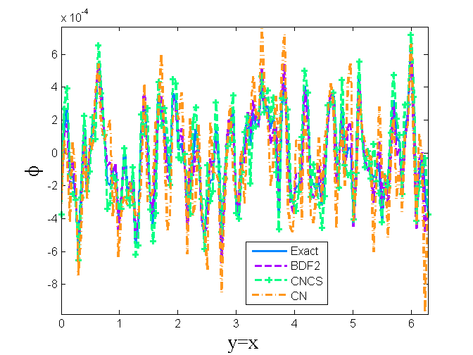
(a) time-step size $\tau=10^{-1}$

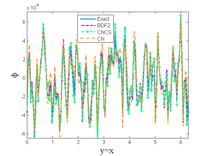
(b) time-step size $\tau=5\times 10^{-2}$

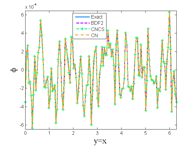
(c) time-step size $\tau=10^{-2}$

Figure 1: Solution curves by BDF2, CN and CNCS methods at $T=0.1$.

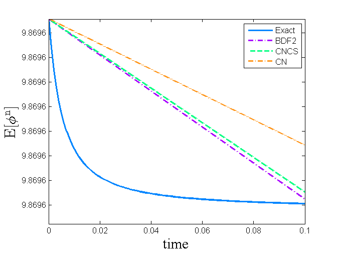
(a) time-step size $\tau=10^{-1}$

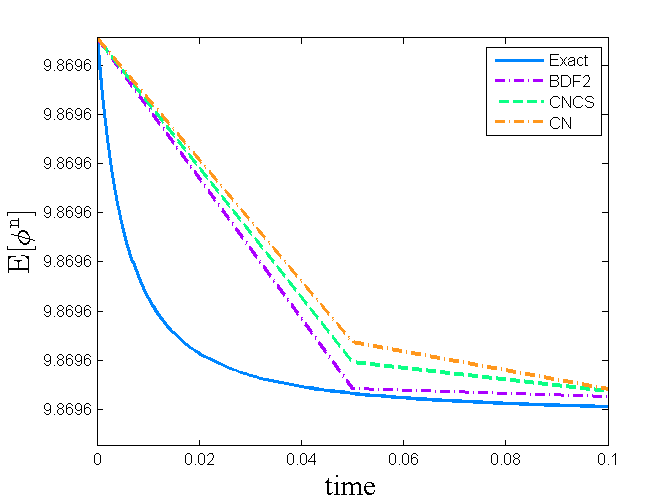
(b) time-step size $\tau=5\times 10^{-2}$

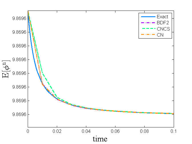
(c) time-step size $\tau=10^{-2}$

Figure 2: Original energy curves by BDF2, CN and CNCS methods until $T=0.1$.

Example 2.

We next simulate the coarsening dynamics of the CH equation (1.2). Precisely, the initial condition is taken as $\Phi_{0}(\mathbf{x})=\text{rand}(\mathbf{x})$, where $\text{rand}(\mathbf{x})$ generates random numbers between $-0.001$ to $0.001$ uniformly. Here, the mobility coefficient $\kappa=2\times 10^{-3}$ and the interfacial thickness $\epsilon=5\times 10^{-2}$ are taken in the following numerical simulations. Always, the spatial domain $(0,2\pi)^{2}$ is discretized by using $128^{2}$ spatial meshes.

5.2 Numerical comparisons

To further benchmark the convex-splitting BDF2 scheme with the random initial data generated in Example 2, we run several numerical tests to explore the numerical behaviors near the initial time. We also implement the unconditionally energy stable Crank-Nicolson (CN) method [31],

$$\partial_{\tau}\phi^{n} =\kappa\Delta_{h}\mu^{n-\frac{1}{2}}\quad\text{with}\quad\mu^{n-\frac{1}{2}}=\frac{1}{2}\big{[}(\phi^{n})^{2}+(\phi^{n-1})^{2}\big{]}\phi^{n-\frac{1}{2}}-\phi^{n-\frac{1}{2}}-\varepsilon^{2}\Delta_{h}\phi^{n-\frac{1}{2}},$$

and the second-order Crank-Nicolson convex-splitting (CNCS) method [8, 13],

$$\partial_{\tau}\phi^{n} =\kappa\Delta_{h}\hat{\mu}^{n-\frac{1}{2}}\quad\text{with}\quad\hat{\mu}^{n-\frac{1}{2}}=\frac{1}{2}\big{[}(\phi^{n})^{2}+(\phi^{n-1})^{2}\big{]}\phi^{n-\frac{1}{2}}-\check{\phi}^{n-\frac{1}{2}}-\varepsilon^{2}\Delta_{h}\hat{\phi}^{n-\frac{1}{2}},$$

where $\phi^{n-\frac{1}{2}}:=(\phi^{n}+\phi^{n-1})/2$, $\hat{\phi}^{n-\frac{1}{2}}:=\left(3\phi^{n}+\phi^{n-2}\right)/4$ and $\check{\phi}^{n-\frac{1}{2}}=\left(3\phi^{n-1}-\phi^{n-2}\right)/2$. Since the CNCS method requires two initialization steps, a first-order convex-splitting scheme [9] is used here to obtain the first-level solution.

The random initial data initiates a fast coarsening dynamics at the beginning time. We use a random initial profile to test the effectiveness of various numerical methods with different time step sizes. The numerical solution curves are summarized in Figure 1, where the reference solution is obtained by using the convex-splitting BDF2 method with a uniform time-step size $\tau=10^{-3}$. We observe that solutions of CN and CNCS methods tend to generate non-physical oscillations when some large time steps are used. In contrast, the convex-splitting BDF2 solution is more robust and accurate than the CN and CNCS schemes with the same time step size. It seems that the BDF2 method is more suitable than Crank-Nicolson type schemes when large time-step sizes are adopted.

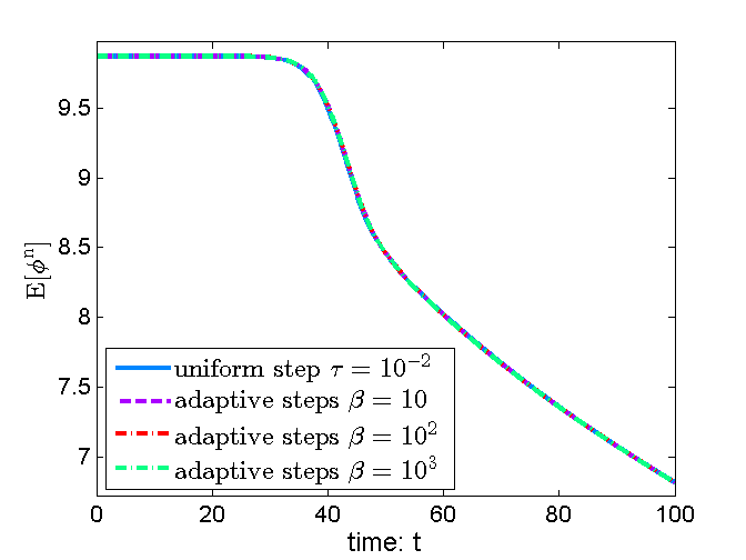
(a) Original energy

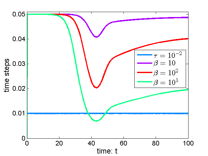
(b) Time step sizes

Figure 3: Energy curves and adaptive time-step sizes for different parameters $\beta$.

Table 2: CPU time (in seconds) and total time steps comparisons.

  Strategies $\tau=10^{-2}$ $\beta=10$ $\beta=10^{2}$ $\beta=10^{3}$ CPU time 109.116 35.601 39.238 71.880 Time levels 10000 2098 2710 5671  

5.3 Simulation of coarsening dynamics

In this subsection, we simulate the coarsening dynamics by using the convex-splitting BDF2 method (1.7) with the random initial condition. In what follows, to capture the multiple time scales accurately and to improve the computational efficiency for long-time simulations, the time steps are selected by using the following adaptive time-stepping strategy [17],

$$\tau_{ada}=\max\Bigg{\{}\tau_{\min},\frac{\tau_{\max}}{\sqrt{1+\beta\big{\|}\partial_{\tau}\phi^{n}\big{\|}^{2}}}\Bigg{\}}\quad\text{so that}\quad\tau_{n+1}=\min\big{\{}\tau_{ada},r_{\mathrm{user}}\tau_{n}\big{\}},$$ (5.1)

where $\beta>0$ is a user chosen parameter, $\tau_{\max}$ and $\tau_{\min}$ are the predetermined maximum and minimum time steps, respectively.

We take $r_{\mathrm{user}}=4$, $\tau_{\min}=5\times 10^{-5}$ and $\tau_{\max}=5\times 10^{-2}$ in the adaptive time-stepping algorithm (5.1), and run the convex-splitting BDF2 method (1.7) until time $T=100$. The reference solution is obtained by applying a small time step $\tau=10^{-2}$. As seen in Figure 3, we use three different user parameters $\beta=10,10^{2}$ and $10^{3}$ to compute the discrete original energy and the corresponding adaptive time-steps. One can observe that the discrete energy curves using the adaptive stepping algorithm are comparable to the reference one. On the other hand, the adjustments of time-steps are closely relied on the user parameter $\beta$. As expected, a large $\beta$ leads to small time-step sizes, and a small $\beta$ generates large step sizes. The CPU time (in seconds) and the adaptive time levels recorded in Table 2 show the effectiveness and efficiency of the adaptive time-stepping algorithm, which makes the long-time dynamics simulations practical.

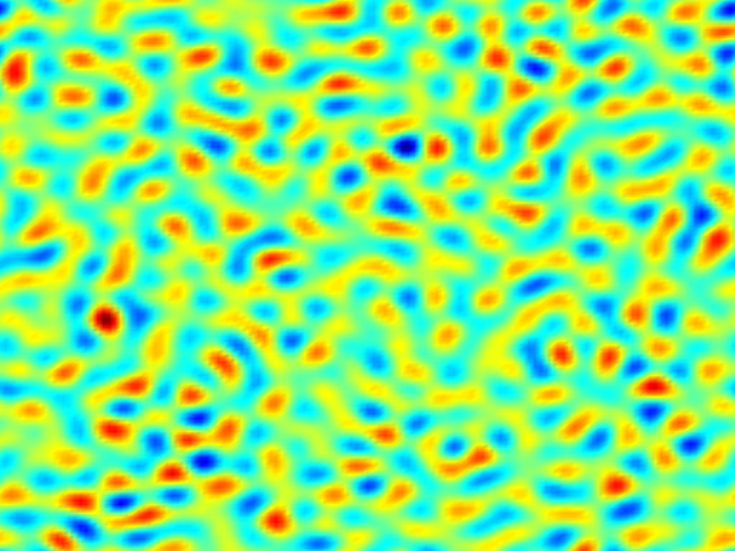
(a) time $t=10$

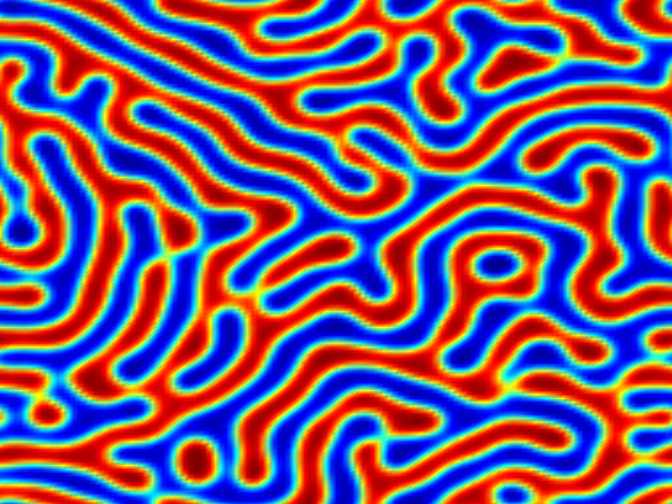
(b) time $t=100$

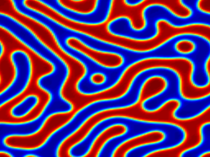
(c) time $t=300$

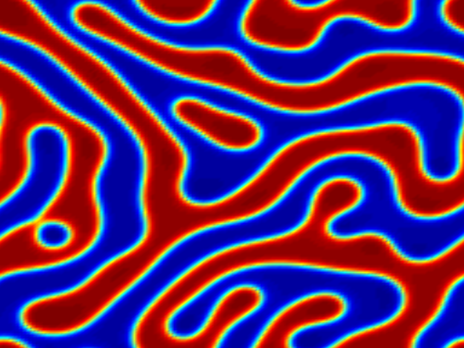
(d) time $t=500$

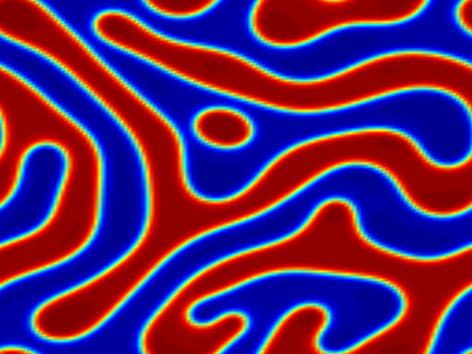
(e) time $t=800$

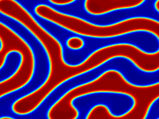
(f) time $t=1000$

Figure 4: The profile of numerical solution $\phi$ at different time for the CH model.

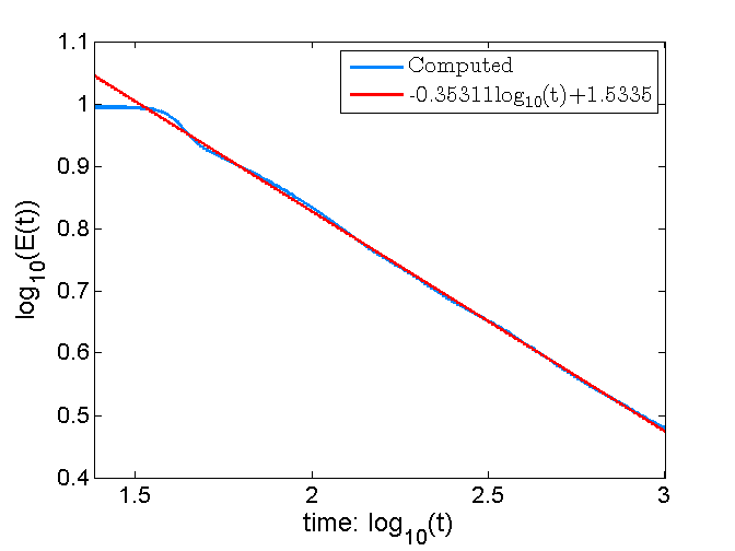
(a) Energy scaling

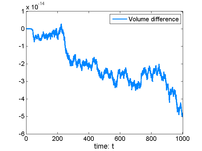
(b) Volume difference

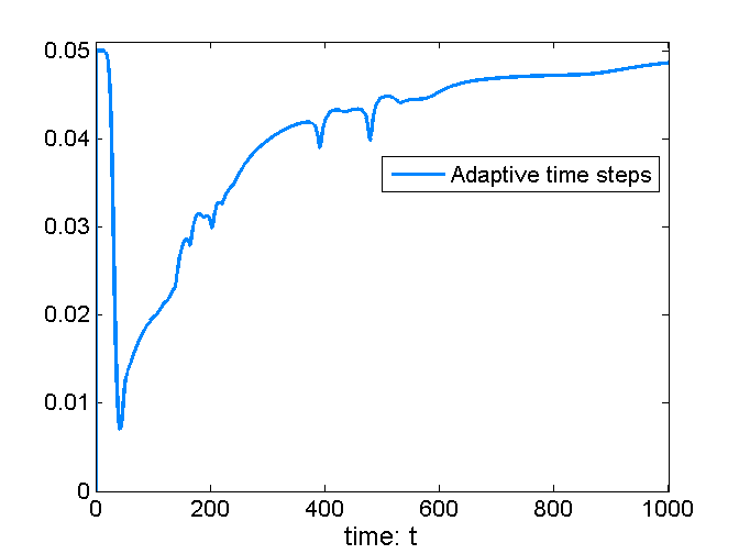
(c) Adaptive step sizes

Figure 5: Numerical results show original energy, volume and adaptive time steps of the CH equation during the coarsening dynamics.

We next perform the coarsening dynamic simulations by using the above adaptive time-stepping strategy with the setting $\beta=10^{3}$ until time $T=1000$. The evolution of microstructure for the CH model due to the phase separation at different time are summarized in Figure 4. As seen, the microstructure is relatively fine and consists of many precipitations at early time. The coarsening, dissolution, merging processes are also observed. The time evolutions of original energy, volume and the adaptive step sizes are summarized in Figure 5. The subplot (a) of Figure 5 demonstrates a very good agreement with the expected scaling law, i.e., the energy decreases as $O(t^{-\frac{1}{3}})$.

References

• [1] J. Becker, A second order backward difference method with variable steps for a parabolic problem, BIT, 38(4) (1998), pp. 644–662.
• [2] A. Bertozzi, S. Esedoglu, and A. Gillette, Inpainting of binary images using the Cahn-Hilliard equation, IEEE Trans. Image Process., 16 (2007), pp. 285–291.
• [3] K. Cheng, W. Feng, C. Wang, and S. Wise, An energy stable fourth order finite difference scheme for the Cahn-Hilliard equation, J. Comput. Appl. Math., 362 (2019), pp. 574–595.
• [4] J. Cahn and J. Hilliard, Free energy of a nonuniform system I. interfacial free energy, J. Chem. Phys., 28 (1958), pp. 258–267.
• [5] V. Cristini, X. Li, J. Lowengrub, and S. Wise, Nonlinear simulations of solid tumor growth using a mixture model: invasion and branching, J. Math. Biol., 58 (2009), pp. 723–763.
• [6] K. Cheng, C. Wang, and S. Wise, An energy stable BDF2 Fourier pseudo-spectral numerical scheme for the square phase field crystal equation, Comm. Comput. Phys., 26(5) (2019), pp. 1335–1364.
• [7] W. Chen, C. Wang, X. Wang, and S. Wise, A linear iteration algorithm for a second-order energy stable scheme for a thin film model without slope selection, J Sci. Comput., 59 (2014), pp. 574–601.
• [8] K. Cheng, C. Wang, S. Wise, and X. Yue, A second-order, weakly energy-stable pseudo-spectral scheme for the Cahn-Hilliard equation and its solution by the homogeneous linear iteration method, J. Sci. Comput., 69 (2016), pp. 1083–1114.
• [9] W. Chen, X. Wang, Y. Yan and Z. Zhang, A second order BDF numerical scheme with variable steps for the Cahn–Hilliard equation, SIAM J. Numer. Anal., 57(1) (2019), pp. 495–525.
• [10] E. Emmrich, Stability and error of the variable two-step BDF for semilinear parabolic problems, J. Appl. Math. & Computing, 19 (2005), pp. 33–55.
• [11] R.D. Grigorieff, Stability of multistep-methods on variable grids, Numer. Math., 42 (1983), pp. 359–377.
• [12] H. Gomez and T. Hughes, Provably unconditionally stable, second-order time-accurate, mixed variational methods for phase-field models, J. Comput. Phys., 230 (2011), pp. 5310–5327.
• [13] J. Guo, C. Wang, S. Wise and X. Yue, An $H^{2}$ convergence of a second-order convex-spliting, finite difference scheme for the three-dimensional Cahn-Hilliard equation, Commun. Math. Sci., 14(2) (2016), pp. 486–515.
• [14] E. Hairer, S.P. Nørsett and G. Wanner, Solving Ordinary Differential Equations I: Nonstiff Problems, Volume 8 of Springer Series in Computational Mathematics, Second Edition, Springer-Verlag, 1992.
• [15] Y. He, Y. Liu and T. Tang, On large time-stepping methods for the Cahn-Hilliard equation, Appl. Numer. Math., 57 (2007), pp. 616-628.
• [16] M.E. Hosea and L.F. Shampine, Analysis and implementation of TR-BDF2, Appl. Numer. Math., 20 (1996), pp. 21-37.
• [17] J. Huang, C. Yang, and Y. Wei, Parallel energy-stable solver for a coupled Allen–Cahn and Cahn–Hilliard system, SIAM J. Sci. Comput., 42(5) (2020), pp. C294–C312.
• [18] H.-L. Liao, B. Ji and L. Zhang, An adaptive BDF2 implicit time-stepping method for the phase field crystal model, IMA J. Numer. Anal., 2020, doi:10.1093/imanum/draa075.
• [19] H.-L. Liao, X. Song, T. Tang and T. Zhou, Analysis of the second order BDF scheme with variable steps for the molecular beam epitaxial model without slope selection, Sci. China Math., 64(5) (2021), pp. 887-902.
• [20] H.-L. Liao, T. Tang and T. Zhou, On energy stable, maximum-principle preserving, second order BDF scheme with variable steps for the Allen-Cahn equation, SIAM J. Numer. Anal., 58(4) (2020), pp. 2294-2314.
• [21] H.-L. Liao, T. Tang and T. Zhou, Positive definiteness of real quadratic forms resulting from variable-step approximations of convolution operators, arXiv:2011.13383v1, 2020.
• [22] H.-L. Liao and Z. Zhang, Analysis of adaptive BDF2 scheme for diffusion equations, Math. Comp., 90 (2020), pp. 1207–1226.
• [23] H. Nishikawa, On large start-up error of BDF2, J. Comput. Phys., 392 (2019), pp. 456–461.
• [24] Z. Qiao, Z. Zhang and T. Tang, An adaptive time-stepping strategy for the molecular beam epitaxy models, SIAM J. Sci. Comput., 33(3) (2011), pp. 1395–1414.
• [25] J. Shen, T. Tang, and L. Wang, Spectral methods: Algorithms, analysis and applications, Springer-Verlag, Berlin Heidelberg, 2011.
• [26] J. Shen, C. Wang, X. Wang and S.M. Wise, Second-order convex-splitting schemes for gradient flows with Ehrlich–Schwoebel type energy: application to thin film epitaxy, SIAM J. Numer. Anal., 50(1) (2012), pp. 105–125.
• [27] G. Tumolo and L. Bonaventura, A semi-implicit, semi-Lagrangian, DG framework for adaptive numerical weather prediction, Quarterly Journal of the Royal Meteorological Society, DOI: 10.1002/qj.2544, 2015.
• [28] W. Wang, Y. Chen and H. Fang, On the variable two-step IMEX BDF method for parabolic integro-differential equations with nonsmooth initial data arising in finance, SIAM J. Numer. Anal., 57(3) (2019), pp. 1289–1317.
• [29] L. Wang and H. Yu, On efficient second order stabilized semi-implicit schemes for the Cahn-Hilliard phase-field equation, J. Sci. Comput., 77 (2018), pp. 1185–1209.
• [30] C. Xu and T. Tang, Stability analysis of large time-stepping methods for epitaxial growth models, SIAM J. Numer. Anal., 44(4) (2006), pp. 1759–1779.
• [31] Z. Zhang and Z. Qiao, An adaptive time-stepping strategy for the Cahn-Hilliard equation, Comm. Comput. Phys., 11(4) (2012), pp. 1261–1278.