On Procrustes Analysis in Hyperbolic Space

Abstract

Congruent Procrustes analysis aims to find the best matching between two point sets through rotation, reflection and translation. We formulate the Procrustes problem for hyperbolic spaces, review the canonical definition of the center of point sets, and give a closed form solution for the optimal isometry for noise-free measurements. We also analyze the performance of the proposed method under measurement noise.

I Introduction

In Greek mythology, Procrustes was a robber who lived in Attica and deformed his victims to match the size of his bed. In 1962, Hurley and Catell used the story of Procrustes to describe a point set matching problem in Euclidean spaces [9], stated below.

Problem 1.

Let $\left\{z_{n}\right\}_{n=1}^{N}$ and $\left\{z^{\prime}_{n}\right\}_{n=1}^{N}$ be two point sets in ${\mathbb{R}}^{d}$. The Procrustes problem asks to find a map $\widehat{T}$ that minimizes the sum of the mismatch norms, i.e.,

$$\widehat{T}=\operatorname*{arg\,min}_{T\in\mathcal{T}}\sum_{n=1}^{N}\left\lVert z_{n}-T(z^{{}^{\prime}}_{n})\right\rVert_{2}^{2}$$

where $\mathcal{T}$ is the set of rotation, reflection, translation, and uniform scaling maps and their compositions [8].

In computer vision, Procrustes analysis is of relevance in point cloud registration problems. The task of rigid registration is to find an isometry between two (or more) sets of points sampled from a $2$ or $3$ dimensional object. Point registration has applications in object recognition [13], medical imaging [6] and localization of mobile robotics  [14]. In signal processing, Procrustes analysis often involved aligning shapes or point sets by a distance preserving bijection. Procrustes problems also naturally arise in distance geometry problems (DGPs) where one wants to find the location of a point set that best represents a given set of incomplete point distances, i.e.,

$$z_{1},\ldots,z_{N}\in{\mathbb{R}}^{d}:\left\lVert z_{n}-z_{m}\right\rVert=d_{mn},\ \forall(m,n)\in\mathcal{M}$$

where $\mathcal{M}\subset\{{1,\ldots,N\}}^{2}$ and $\left\{d_{m,n}:(m,n)\in\mathcal{M}\right\}$ is the set of measured distances [10]. If a distance geometry problem has a solution, it is an orbit of the form

$$O_{\mathcal{Z}}=\left\{\left\{T(z_{n})\right\}_{n=1}^{N}\text{ s.t. }T:{\mathbb{R}}^{d}\rightarrow{\mathbb{R}}^{d}\mbox{ is an isometry}\right\},$$

where $\mathcal{Z}=\left\{z_{n}\right\}_{n=1}^{N}$ is a particular solution. In order to uniquely identify the correct solution from all the possible elements in the orbit $O_{\mathcal{Z}}$, we may be given the exact position of a subset of points, called anchors. We use Procrustes analysis to pick the correct solution by finding the best match between the anchors with their corresponding points in the orbit. This technique is commonly used in localization problems [4, 19].

Procrustes analysis can be performed in any metric space. In particular, hyperbolic Procrustes analysis is of great relevance due to the recent surge of interest in hyperbolic embeddings and machine learning [18, 3]. Furthermore, hyperbolic embeddings are closely connected to the study of hierarchical or tree-like data structures and hyperbolic Procrustes problem solutions may be used to align hierarchical data, e.g., ontologies [17, 5]. The goal of ontological studies is to find a (distance preserving) map between a fixed number of entities in two tree-like structures that are best aligned to each other (see Figure 1 for an illustration). For example, in ontology matching one aims to find correspondences between semantically related entities in heterogeneous ontologies with the goal of ontology merging, query response, or data translation [17].

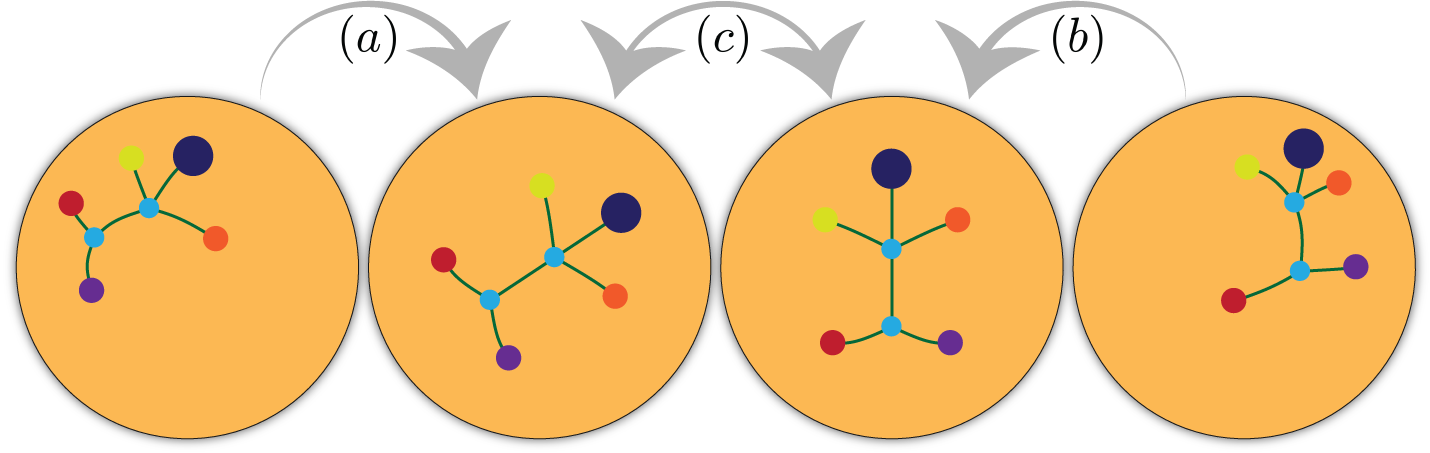
Figure 1: Tree alignment in the Poincaré disk [2]. Hyperbolic Procrustes analysis aims to align two trees, depicted on the far left and far right figures. In steps $(a)$ and $(b)$ we center vertices in both trees, while in step $(c)$ we estimate the unknown rotation map.

In unsupervised matching problems, the first step in Procrustes-type analyses is to find the correspondence between two point clouds by using the iterative closest point algorithm [16]. Recently, Alvarez-Melis et al.  [1] cast the unsupervised hierarchy matching problem in hyperbolic space. Their proposed method jointly learns the soft correspondence and the alignment map characterized by a hyperbolic neural network.

In our work, we start with parametric isometries in the ’Loid model of hyperbolic spaces. It is known that one can decompose any isometry into elementary isometries, e.g., hyperbolic translations and hyperbolic rotations (and reflections). In our setting, we aim to find a joint estimate for hyperbolic translation and rotation maps that best align two point sets.

To accomplish this task, we review the definition of the center of mass, or centroid, for a set of points in hyperbolic space. This enables us to subsequently center each set, and decouple the joint estimation problem into two steps: $(1)$ translate the center of mass of each point set to the coordinate origin (of the Poincaré model), and $(2)$ estimate the unknown rotation factor. While hyperbolic centering has been studied in the literature [11], our Procrustes analysis framework is different from prior work in so far that it is similar to its Euclidean counterpart, and provides an optimal estimate for the unknown rotation factor, based on the weighted mean of pairwise inner products. Moreover, we prove a proof that our proposed method ensures the theoretically optimal isometry if the point sets match perfectly. We conclude the paper by giving numerical performance bounds for the task of matching noisy point sets.

Notation. For $N\in\mathbb{N}$, we let $[N]=\left\{1,\ldots,N\right\}$. Depending on the context, $x_{1}$ can either be the first element of $x\in{\mathbb{R}}^{d}$, or an indexed vector. We denote the set of orthogonal matrices as $\mathbb{O}(d)=\left\{R\in{\mathbb{R}}^{d\times d}:R^{\top}R=I\right\}$. For a function $f$ and its inputs $x_{1},\ldots,x_{N}$, we write $\overline{f(x_{n})}=\frac{1}{N}\sum_{n\in[N]}f(x_{n})$. For a vector $b\in{\mathbb{R}}^{d}$, we denote its $\ell_{2}$ norm as $\left\lVert b\right\rVert_{2}$.

II ’Loid Model of Hyperbolic Space

Let $x,x^{\prime}\in{\mathbb{R}}^{d+1}$ with $d\geq 1$. The Lorentzian inner product between $x$ and $x^{\prime}$ is defined as

$$[x,x^{\prime}]=x^{\top}Hx^{\prime}:H=\begin{pmatrix}-1&0^{\top}\\ 0&I_{d}\end{pmatrix},$$ (1)

where $I_{d}\in{\mathbb{R}}^{d\times d}$ is the identity matrix. This is an indefinite inner product on ${\mathbb{R}}^{d+1}$. The vector space ${\mathbb{R}}^{d+1}$ equipped with the Lorentzian inner product is called a Lorentzian $(d+1)$-space. In a Lorentzian space, we can define notions similar to adjoint and unitary matrices in Euclidean spaces. The $H$-adjoint of the matrix $R$, denoted by $R^{[*]}$, is defined via

$$[Rx,x^{\prime}]=[x,R^{[*]}x^{\prime}],~{}\forall x,x^{\prime}\in{\mathbb{R}}^{d+1},$$

or simply as $R^{[*]}=H^{-1}R^{\top}H$. An invertible matrix $R$ is called H-unitary if $R^{[*]}=R^{-1}$ [7].

The ’Loid model of $d$-dimensional hyperbolic space is a Riemannian manifold $\mathcal{L}^{d}=({\mathbb{L}}^{d},(g_{x})_{x})$, where

$${\mathbb{L}}^{d}=\left\{x\in{\mathbb{R}}^{d+1}:[x,x]=-1,x_{1}>0\right\}$$

and the Riemannian metric $g_{x}:T_{x}{\mathbb{L}}^{d}\times T_{x}{\mathbb{L}}^{d}\rightarrow{\mathbb{R}}$ defined as $g_{x}(u,v)=[u,v]$. The distance function in the ’Loid model are characterized by Lorentzian inner products as

$$d(x,x^{\prime})=\mathrm{acosh}(-[x,x^{\prime}]),\forall x,x^{\prime}\in{\mathbb{L}}^{d}.$$

II-A Isometries

A map $T:{\mathbb{L}}^{d}\rightarrow{\mathbb{L}}^{d}$ is an isometry if it is bijective and preserves distances, i.e. if

$$d(x,x^{\prime})=d\big{(}T(x),T(x^{\prime})\big{)},~{}\forall x,x^{\prime}\in{\mathbb{L}}^{d}.$$

We can represent any hyperbolic isometry as a composition of two elementary maps that are parameterized by a $d$-dimensional vector and a $d\times d$ unitary matrix, as described below.

Fact 1.

[15] The function $T:{\mathbb{L}}^{d}\rightarrow{\mathbb{L}}^{d}$ is an isometry if and only if it can be written as $T(x)=R_{U}R_{b}x$, where

$$R_{U}=\left[\begin{array}[]{cc}1&0^{\top}\\ 0&U\end{array}\right],\ R_{b}=\left[\begin{array}[]{cc}\sqrt{1+\left\lVert b\right\rVert_{2}^{2}}&b^{\top}\\ b&(I+bb^{\top})^{\frac{1}{2}}\end{array}\right]$$

for a unitary matrix $U\in\mathbb{O}(d)$ and a vector $b\in{\mathbb{R}}^{d}$.

1 can be directly verified by finding the conditions for a real matrix $R$ to be $H$-unitary, i.e., $R^{\top}HR=H$ or simply $R=H^{-\frac{1}{2}}CH^{\frac{1}{2}}\in{\mathbb{R}}^{(d+1)\times(d+1)}$ where $C^{\top}C=I$ and $C\in\mathbb{C}^{(d+1)\times(d+1)}$. We use this parametric decomposition of rigid transformations to solve the Procrustes problem in ${\mathbb{L}}^{d}$.

Fact 2.

$T_{b}^{-1}=T_{-b}$ and $T_{U}^{-1}=T_{U^{\top}}$ where $b\in{\mathbb{R}}^{d}$ and $U\in\mathbb{O}(d)$.

The hyperbolic translation map $T_{b}:{\mathbb{L}}^{d}\rightarrow{\mathbb{L}}^{d}$ and hyperbolic rotation map $T_{U}:{\mathbb{L}}^{d}\rightarrow{\mathbb{L}}^{d}$ are defined as

$$T_{b}(x) =R_{b}x, \mbox{for}\ b\in{\mathbb{R}}^{d},$$ (2)

$$T_{U}(x) =R_{U}x, \mbox{for}\ U\in\mathbb{O}(d).$$ (3)

III Procrustes Analysis

Euclidean (orthogonal) Procrustes analysis proceeds through two steps:

• Centering: moving the center of mass of both points set to the origin of Cartesian coordinates, and

• Finding the optimal rotation/reflection.

We proceed to review (and visualize) the definition of the center of mass of a point set in hyperbolic space [11, Chapter 13].

We start by projecting each point $x\in{\mathbb{L}}^{d}$ onto the following $d$-dimensional subspace

$$H_{d}=\left\{x\in{\mathbb{R}}^{d+1}:x_{1}=0\right\}.$$

Then, we can simply neglect the first element of the projected point (which is always zero), and define a one-to-one map $\mathcal{P}$ between ${\mathbb{L}}^{d}$ and ${\mathbb{R}}^{d}$; see Figure 2. In Definition 1, we formalize this projection and its inverse.

Definition 1.

The projection operator $\mathcal{P}:{\mathbb{L}}^{d}\rightarrow{\mathbb{R}}^{d}$ and its inverse ${\mathcal{Q}}$ are defined as

$$\mathcal{P}\Big{(}\left[\begin{array}[]{c}\sqrt{1+\left\lVert z\right\rVert^{2}}\\ z\end{array}\right]\Big{)}=z,\ {\mathcal{Q}}(z)=\begin{bmatrix}\sqrt{1+\left\lVert z\right\rVert^{2}}\\ z\end{bmatrix}.$$

For brevity, we define ${\mathcal{P}}(X)\overset{\text{def}}{=}[{\mathcal{P}}(x_{1}),\ldots,{\mathcal{P}}(x_{N})]$ where $X=[x_{1},\ldots,x_{N}]\in({\mathbb{L}}^{d})^{N}$. Similarly, we consider this extension for ${\mathcal{Q}}$ as well.

In Section III-A, we review the hyperbolic centering process [11]. In other words, we find a map $T_{b}$ to move the center of mass of projected point sets to $0\in{\mathbb{R}}^{d}$, i.e., $\overline{{\mathcal{P}}\big{(}T_{b}(x_{n})\big{)}}=0$. Then, we show how this centering method helps simplify the hyperbolic Procrustes problem to a sub-problem similar to the famous (Euclidean) orthogonal Procrustes problem.

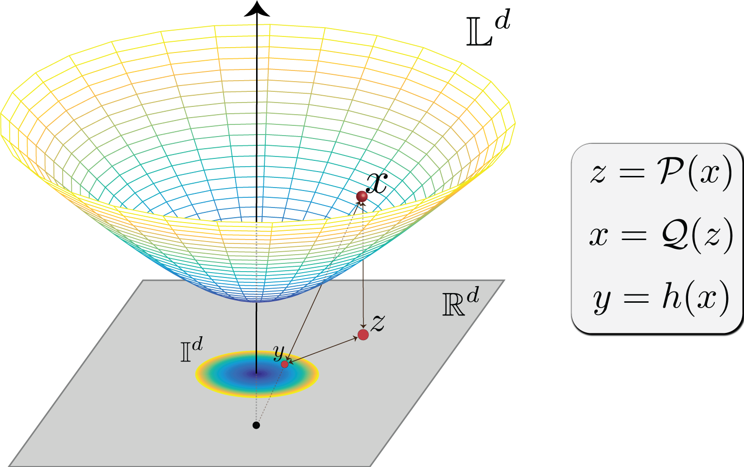
Figure 2: Geometric illustration of ${\mathcal{P}}$, ${\mathcal{Q}}$, and stereographic projection $h$.

III-A Hyperbolic Centering

In Euclidean Procrustes analysis, we have two point sets $z_{1},\ldots,z_{N}$ and $z^{\prime}_{1},\ldots z^{\prime}_{N}$ that are related via a composition of rotation, reflection, and translation maps, i.e.,

$$z_{n}=Uz^{\prime}_{n}+b$$

where $U\in\mathbb{O}(d)$ and $b\in{\mathbb{R}}^{d}$. We extract translation invariant features by moving their point mass to $0\in{\mathbb{R}}^{d}$, i.e.,

$$z_{n}-\overline{z_{n}}=U(z^{\prime}_{n}-\overline{z^{\prime}_{n}}).$$

The main purpose of centering is to map each point set to new locations, $z_{n}-\overline{z_{n}}$ and $z^{\prime}_{n}-\overline{z^{\prime}_{n}}$ that are invariant with respect to the unknown translation $b$. Subsequently, we can estimate the unknown unitary matrix $\hat{U}$, and then the translation according to $\widehat{b}=\overline{z_{n}}-\widehat{U}\overline{z^{\prime}_{n}}$.

In hyperbolic Procrustes analysis, we have

$$x_{n}=R_{b}R_{U}x^{\prime}_{n},\forall n\in[N]$$ (4)

where $U\in\mathbb{O}(d)$ and $b\in{\mathbb{R}}^{d}$. In a similar way, we pre-process a point set to extract (hyperbolic) translation invariant locations, i.e., centered point sets. Lemma 1 gives a simple method to center a projected point set.

Lemma 1.

[11] Let $x_{1},x_{2},\ldots,x_{N}\in{\mathbb{L}}^{d}$. Then, we have

$$\overline{{\mathcal{P}}\big{(}R_{-m_{x}}x_{n}\big{)}}=0$$

where $m_{x}\overset{\text{def}}{=}\frac{1}{\sqrt{-[\overline{x_{n}},\overline{x_{n}}]}}\ \overline{{\mathcal{P}}(x_{n})}$.

In Proposition 1, we show that $T_{-m_{x}}$ is the canonical translation map for centering the point set $X\in\big{(}{\mathbb{L}}^{d}\big{)}^{N}$.

Proposition 1.

Let $x_{1},\ldots,x_{N}$ and $x^{\prime}_{1},\ldots x^{\prime}_{N}$ in ${\mathbb{L}}^{d}$ such that

$$x_{n}=R_{b}R_{U}x^{\prime}_{n},\ \forall n\in[N].$$

for $b\in{\mathbb{R}}^{d}$ and $U\in\mathbb{O}(d)$. Then, $R_{-m_{x}}x_{n}=R_{V}R_{-m_{x^{\prime}}}x_{n}^{\prime}$ where $R_{V}$ is a hyperbolic rotation matrix.

Proof.

From Lemma 1, we have

$$\overline{R_{-m_{x}}x_{n}}=\left[\begin{array}[]{c}a_{1}\\ 0\end{array}\right],\overline{R_{-m_{x^{\prime}}}x^{\prime}_{n}}=\left[\begin{array}[]{c}a_{2}\\ 0\end{array}\right]$$

for $a_{1},a_{2}\in{\mathbb{R}}$. On the other hand, we can rewrite eq. 4 in the following form

$$R_{-m_{x}}x_{n}=R^{\prime}R_{-m_{x^{\prime}}}x_{n}^{\prime},\forall n\in[N].$$

where $R^{\prime}=R_{-m_{x}}R_{b}R_{U}R_{m_{x^{\prime}}}$. Since $R^{\prime}$ is an $H$-unitary matrix, we can decompose it as $R^{\prime}=R_{c}R_{V}$ for some $c\in{\mathbb{R}}^{d}$ and $V\in\mathbb{O}(d)$. Therefore, we have

$$\left[\begin{array}[]{c}a_{1}\\ 0\end{array}\right]=R_{c}R_{V}\left[\begin{array}[]{c}a_{2}\\ 0\end{array}\right].$$

This gives $c=0$. ∎

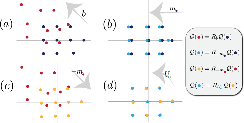
Figure 3: $(a)$: Red and blue are projected points related by a translation, i.e., $X=R_{b}X^{\prime}$. $(b,c)$: Centering each point set. $(d)$: Centered points are related via a rotation, i.e., $R_{m_{x}}R_{b}R_{-m_{x^{\prime}}}\neq I_{d}$.

The map $T_{-m_{x}}$ not only centers a set of points, but also rotates them. This phenomena is rooted in the noncommutative property of hyperbolic translation or gyration. More clearly, for any two vectors $b_{1},b_{2}\in{\mathbb{R}}^{d}$, we have

$$R_{b_{1}}R_{b_{2}}=R_{V}R_{b_{2}}R_{b_{1}}$$

for a specific unitary matrix $V\in\mathbb{O}(d)$ that accounts for the gyration factor; see the example in Figure 3 and the follow-up discussion in Section IV. This does not interfere with our analysis since any such rotation is absorbed in $U$, and as we can estimate their joint unitary transformation.

Now, let us consider the following noisy case,

$$x_{n}=R_{b}R_{U}R_{\epsilon_{n}}x^{\prime}_{n},\ \forall n\in[N]$$

where $\epsilon_{n}\in{\mathbb{R}}^{d}$ is a translation noise for the point $x^{\prime}_{n}$. Let $z_{n}=R_{\epsilon_{n}}x^{\prime}_{n}$. Then we have $R_{-m_{x}}x_{n}=R_{V}R_{-m_{z}}z_{n}$. The centroid $m_{z}$ is related to $m_{x^{\prime}}$ and $\left\{\epsilon_{n}\right\}_{n\in[N]}$. Therefore, we can write $m_{z}=m_{x^{\prime}}+\epsilon$ for a $\epsilon\in{\mathbb{R}}^{d}$. This leads to

$$R_{-m_{x}}x_{n}=R_{V}R_{\epsilon^{\prime}_{n}}R_{-m_{x^{\prime}}}x^{\prime}_{n},\ \forall n\in[N],$$

where $R_{\epsilon^{\prime}_{n}}=R_{-m_{x^{\prime}}-\epsilon}R_{\epsilon_{n}}R_{m_{x^{\prime}}}$. If the translation noise of each point is sufficiently small, then $R_{V}R_{\epsilon^{\prime}_{n}}\approx R_{V^{\prime}}$ for a $V^{\prime}\in\mathbb{O}(d)$.

III-B Hyperbolic Rotation & Reflection

To estimate the unknown hyperbolic rotation, we consider minimizing a weighted discrepancy between the centered point sets. More precisely,

$$\widehat{U}=\operatorname*{arg\,min}_{V\in\mathbb{O}(d)}\sum_{n\in[N]}w_{n}f\Big{(}d\big{(}R_{-m_{x}}x_{n},R_{V}R_{-m_{x^{\prime}}}x^{\prime}_{n}\big{)}\Big{)}$$ (5)

where $d(x,x^{\prime})={\mathrm{acosh}}(-x^{\top}Hx^{\prime})$, $\left\{w_{n}\right\}_{n\in[N]}$ are positive weights, and $f(\cdot)=\cosh(\cdot)$ is a monotonic function.

Proposition 2.

The optimal unitary matrix that solves (5) equals $\widehat{U}=U_{l}U_{r}^{\top}$, where $U_{l}\Sigma U_{r}^{\top}$ is the singular value decomposition of ${\mathcal{P}}(R_{-m_{x}}X)W{\mathcal{P}}(R_{-m_{x^{\prime}}}X^{\prime})^{\top}$, and $W=\mathrm{diag}(w_{1},\ldots,w_{N})$.

Proof.

We can simplify (5) as follows:

$$\widehat{U}=\operatorname*{arg\,max}_{V\in\mathbb{O}(d)}\sum_{n\in[N]}\mathop{\mathrm{Tr}}R_{-m_{x^{\prime}}}x^{\prime}_{n}w_{n}(R_{-m_{x}}x_{n})^{\top}HR_{V}.$$

From 1, we know that $R_{V}$ is only parameterized on its lower right block. The proof then follows from representing the sum in matrix form and invoking von Neumann’s trace inequality [12]. ∎

IV Möbius addition

In the Poincaré model (${\mathbb{I}}^{d}$), the points reside in the unit $d$-dimensional Euclidean ball. The isometry between the ’Loid and the Poincaré model $h:{\mathbb{L}}^{d}\rightarrow{\mathbb{I}}^{d}$ is called the stereographic projection [2]. The distance between $y,y^{\prime}\in{\mathbb{I}}^{d}$ is given by $d(y,y^{\prime})=2\mathrm{tanh}^{-1}(\left\lVert-y\oplus y^{\prime}\right\rVert)$ where $\oplus$ is Möbius addition — a noncommutative and nonassociative operator. Gyration measures the deviation of Möbius addition from commutativity, i.e., $\mathrm{gyr}[y,y^{\prime}](y^{\prime}\oplus y)=y\oplus y^{\prime}$ [20].

Fact 3.

The maps $h\circ R_{U}\circ h^{-1}$ and $h\circ T_{U}\circ h^{-1}$ are isometries in the Poincaré model, and they can be written as

$$h\circ T_{U}\circ h^{-1}(y)=Uy,\ \ h\circ T_{b}\circ h^{-1}(y)=b^{\prime}\oplus y$$

where $b^{\prime}=h\circ{\mathcal{Q}}(b)$, $T_{b}$ and $T_{U}$ are defined in (2) and (3).

The translation isometry is a direct result of the Gyrotranslation theorem equality,

$$-(c\oplus y)\oplus c\oplus y^{{}^{\prime}}=\mathrm{gyr}[c,y](-y\oplus y^{\prime}),$$

where $c\in{\mathbb{I}}^{d}$ [20]. Therefore, left Möbius addition preserves the distances of point sets in the Poincaré model. We can hence perform a Procrustes analysis in the Poincaré model by $(1)$ centering each point set, i.e., subtracting their center of mass from the left hand side of the Möbius addition, and $(2)$ estimating the remaining rotation factor — a composition of gyrations and the initial unknown rotation between the two point sets.

V Numerical Analysis

Let $x_{n}=R^{*}R_{\epsilon_{n}}x^{\prime}_{n},\ \forall n\in[N]$ where $R^{*}$ is an $H$-unitary matrix and $\epsilon_{1},\ldots,\epsilon_{N}$ is the set of translation noise samples.

We compute the following $H$-unitary operators to match the point sets $X,X^{\prime}$:

• $R_{P}$: The matrix estimated by our proposed method;

• $R_{\mathrm{GD}}$: Let $e(X,\overline{X})\overset{\text{def}}{=}\frac{1}{Nd}\sum_{n\in[N]}d(x_{n},\overline{x}_{n})$ be the normalized discrepancy between $X$ and $\overline{X}$. The matrix $R_{\mathrm{GD}}$ is computed by an iterative gradient descent method: We initialize $R_{\mathrm{GD}}=I_{d+1}$, and iterate the following steps: $(1)$ $\widehat{b}=-\alpha\frac{\partial}{\partial b}e(X,R_{b}R_{\mathrm{GD}}X^{\prime})|_{b=0}$ for a small $\alpha>0$; $(2)$ $\widehat{U}=\operatorname*{arg\,max}_{U\in\mathbb{O}(d)}\sum_{n\in[N]}[x_{n},R_{U}R_{\widehat{b}}R_{\mathrm{GD}}x^{\prime}_{n}]$; $(3)$ Update $R_{\mathrm{GD}}\leftarrow R_{\widehat{U}}R_{\widehat{b}}R_{\mathrm{GD}}$;

• $R_{\mathrm{GD+P}}$: We can combine the aforementioned methods by $(1)$ solving the problem with our method, and $(2)$ fine-tuning the estimated isometry by applying the gradient method on the point sets $X$ and $R_{P}X^{\prime}$.

For a random $H$-unitary $R^{*}$ and all $n\in[N]$, we sample $d$-dimensional $z_{n}\sim\mathcal{N}(0,I)$, and $\epsilon_{n}\sim 10^{-2}\mathcal{N}(0,I)$; Then, we let $x^{\prime}_{n}=\mathcal{Q}(z_{n})$ and $x_{n}=R^{*}R_{\epsilon_{n}}x^{\prime}_{n}$. For $10^{3}$ random $(X,X^{\prime})$ pairs, we compute their normalized discrepancy $e(X,RX^{\prime})$, where $R\in\left\{R_{P},R_{\mathrm{GD}},R_{\mathrm{GD+P}}\right\}$. All methods successfully denoise the measurements, i.e., $e(X,R^{*}X^{\prime})>e(X,RX^{\prime})$; see Figure 4 $(a)$. We should note that the gradient descent method does not necessarily converge to an acceptable solution. Therefore, we report the number of outlier trials, i.e.,

$$(X,X^{\prime}):|e(X,RX^{\prime})-Q_{2}|>k\frac{1}{2}|Q_{3}-Q_{1}|$$ (6)

where $Q_{1},Q_{2}$ and $Q_{3}$ are first, second and third quartiles of the total reported discrepancies, and $k=5$ for a conservative criterion to pick outliers (see  Figure 4 $(b)$). The gradient descent method has the most number of outlier whereas our proposed method has the minimum number of outliers — comparable to outliers in the measurement noise. Therefore, the proposed method robustly solves the hyperbolic Procrustes problem and its accuracy can be moderately improved with a post fine-tuning gradient method.

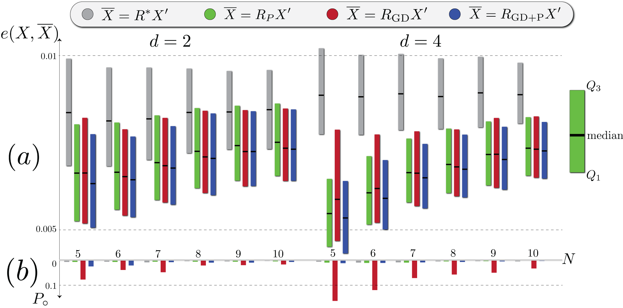
Figure 4: $(a)$ Normalized discrepancy for random hyperbolic point sets of size $N\in\left\{5,\ldots,10\right\}$ and dimensions $d\in\left\{2,4\right\}$. For $10^{3}$ trials, we report the quartiles $Q_{1},Q_{2}$ and $Q_{3}$ since they are robust to outliers. $(b)$ The probability of an outlier event $P_{\circ}=10^{-3}\times\mbox{total number of outliers}$, e.g., the fraction of examples that failed to converge or outlier defined in the sense of  (6).

VI Conclusion

Inspired by its Euclidean counterpart, we introduced the Procrustes problem in hyperbolic spaces. We reviewed the (indefinite) Lorentizian inner product, and described how $H$-unitary matrices represent isometries in the ’Loid model of hyperbolic spaces. Using the parameterized decomposition of hyperbolic isometries in terms of hyperbolic rotation and translation, we showed that moving the center of mass to the origin gives point sets that are invariant to hyperbolic translation (for the case of no measurement noise). We then used the centered point sets to estimate the unknown rotation factor.

VII Acknowledgment

The authors would like to thank Prof. Olgica Milenkovic for helpful discussions and suggestions.

References

- Alvarez-Melis et al. [2020] David Alvarez-Melis, Youssef Mroueh, and Tommi Jaakkola. Unsupervised hierarchy matching with optimal transport over hyperbolic spaces. In International Conference on Artificial Intelligence and Statistics, pages 1606–1617. PMLR, 2020.
- Cannon et al. [1997] James W Cannon, William J Floyd, Richard Kenyon, Walter R Parry, et al. Hyperbolic geometry. Flavors of geometry, 31:59–115, 1997.
- De Sa et al. [2018] Christopher De Sa, Albert Gu, Christopher Ré, and Frederic Sala. Representation tradeoffs for hyperbolic embeddings. Proceedings of machine learning research, 80:4460, 2018.
- Dokmanic et al. [2015] Ivan Dokmanic, Reza Parhizkar, Juri Ranieri, and Martin Vetterli. Euclidean distance matrices: essential theory, algorithms, and applications. IEEE Signal Processing Magazine, 32(6):12–30, 2015.
- Euzenat et al. [2007] Jérôme Euzenat, Pavel Shvaiko, et al. Ontology matching, volume 18. Springer, 2007.
- Fitzpatrick et al. [1998] J Michael Fitzpatrick, Jay B West, and Calvin R Maurer. Predicting error in rigid-body point-based registration. IEEE transactions on medical imaging, 17(5):694–702, 1998.
- Gohberg et al. [1983] Israel Gohberg, Peter Lancaster, and Leiba Rodman. Matrices and indefinite scalar products. 1983.
- Gower [1975] John C Gower. Generalized procrustes analysis. Psychometrika, 40(1):33–51, 1975.
- Hurley and Cattell [1962] John R Hurley and Raymond B Cattell. The procrustes program: Producing direct rotation to test a hypothesized factor structure. Behavioral science, 7(2):258, 1962.
- Liberti et al. [2014] Leo Liberti, Carlile Lavor, Nelson Maculan, and Antonio Mucherino. Euclidean distance geometry and applications. SIAM review, 56(1):3–69, 2014.
- Mardia and Jupp [2009] Kanti V Mardia and Peter E Jupp. Directional statistics, volume 494. John Wiley & Sons, 2009.
- Mirsky [1975] Leon Mirsky. A trace inequality of john von neumann. Monatshefte für mathematik, 79(4):303–306, 1975.
- Mitra et al. [2004] Niloy J Mitra, Natasha Gelfand, Helmut Pottmann, and Leonidas Guibas. Registration of point cloud data from a geometric optimization perspective. In Proceedings of the 2004 Eurographics/ACM SIGGRAPH symposium on Geometry processing, pages 22–31, 2004.
- Pomerleau et al. [2015] François Pomerleau, Francis Colas, and Roland Siegwart. A review of point cloud registration algorithms for mobile robotics. 2015.
- Ratcliffe et al. [2006] John G Ratcliffe, S Axler, and KA Ribet. Foundations of hyperbolic manifolds, volume 149. Springer, 2006.
- Rusinkiewicz and Levoy [2001] Szymon Rusinkiewicz and Marc Levoy. Efficient variants of the icp algorithm. In Proceedings third international conference on 3-D digital imaging and modeling, pages 145–152. IEEE, 2001.
- Shvaiko and Euzenat [2011] Pavel Shvaiko and Jérôme Euzenat. Ontology matching: state of the art and future challenges. IEEE Transactions on knowledge and data engineering, 25(1):158–176, 2011.
- Tabaghi and Dokmanić [2020] Puoya Tabaghi and Ivan Dokmanić. Hyperbolic distance matrices. In Proceedings of the 26th ACM SIGKDD International Conference on Knowledge Discovery & Data Mining, KDD ’20, page 1728–1738. Association for Computing Machinery, 2020. ISBN 9781450379984.
- Tabaghi et al. [2019] Puoya Tabaghi, Ivan Dokmanić, and Martin Vetterli. Kinetic euclidean distance matrices. IEEE Transactions on Signal Processing, 68:452–465, 2019.
- Ungar [2008] Abraham Albert Ungar. A gyrovector space approach to hyperbolic geometry. Synthesis Lectures on Mathematics and Statistics, 1(1):1–194, 2008.