SPADE: A Spectral Method for Black-Box Adversarial Robustness Evaluation

Abstract

A black-box spectral method is introduced for evaluating the adversarial robustness of a given machine learning (ML) model. Our approach, named SPADE, exploits bijective distance mapping between the input/output graphs constructed for approximating the manifolds corresponding to the input/output data. By leveraging the generalized Courant-Fischer theorem, we propose a SPADE score for evaluating the adversarial robustness of a given model, which is proved to be an upper bound of the best Lipschitz constant under the manifold setting. To reveal the most non-robust data samples highly vulnerable to adversarial attacks, we develop a spectral graph embedding procedure leveraging dominant generalized eigenvectors. This embedding step allows assigning each data sample a robustness score that can be further harnessed for more effective adversarial training. Our experiments show the proposed SPADE method leads to promising empirical results for neural network models that are adversarially trained with the MNIST and CIFAR-10 data sets.

1 Introduction

Recent research efforts have demonstrated the evident lack of robustness in state-of-the-art machine learning (ML) models—e.g., a visually imperceptible adversarial image can be crafted via an optimization procedure to mislead a well-trained deep neural network (DNN) (Szegedy et al., 2013; Goodfellow et al., 2014). Consequently, it is becoming increasingly important to effectively assess and improve the adversarial robustness of ML models for safety-critical applications, such as autonomous driving systems. To this end, a variety of white-box approaches has been proposed. For instance, study in (Szegedy et al., 2013) proposed a layer-wise global Lipschitz constant estimation approach, which provides a loose bound on robustness evaluation; (Hein & Andriushchenko, 2017) introduced a method for assessing the lower bound of model robustness based on local Lipschitz continuous condition for a multilayer perceptron (MLP) with a single hidden layer; (Weng et al., 2018) proposed a method for estimating local Lipschitz constant based on extreme value theory. However, most existing adversarial robustness evaluation frameworks are based on white-box methods which assume the model parameters are given in advance. For example, the recent CLEVER algorithm for adversarial robustness evaluation (Weng et al., 2018) requires full access to the gradient information of a given neural network for estimating a universal lower bound on the minimal distortion required to craft an adversarial example from an original one.

This work introduces SPADE , a black-box method for evaluating adversarial robustness by only using the input (features) and output vectors of the ML model. Essentially, our method evaluates adversarial robustness through checking if there exist two nearby input data samples that can be mapped to very distant output ones by the underlying function of the ML model; if so, we have a large distance mapping distortion (DMD), which implies potentially poor adversarial robustness since a small perturbation applied to these inputs can lead to rather significant changes on the output side. To allow meaningful distance comparisons of input/output data samples in a high-dimensional space, our approach leverages graph-based manifolds and focuses on resistance distance metric for adversarial robustness evaluations. The main contributions of this work are as follows:

$\bullet$ To our knowledge, we are the first to introduce a black-box spectral method (SPADE) for adversarial robustness evaluation of an ML model by examining the bijective distance mappings between the input/output graph-based manifolds.

$\bullet$ We show that the largest generalized eigenvalue (i.e., SPADE score) computed with the input/output graph Laplacians can be a good surrogate (upper bound) for the best Lipschitz constant of the underlying function, which thus can be leveraged for quantifying the adversarial robustness.

$\bullet$ We propose a spectral graph embedding scheme leveraging the generalized Courant-Fischer theorem for estimating the robustness of each data point: a data point with a larger SPADE score means it may contain a greater amount of non-robust features, and thus can be more vulnerable to adversarial perturbations.

$\bullet$ We show that the SPADE score of an ML model can be directly used as a black-box metric for quantifying its adversarial robustness. Moreover, by taking advantage of the SPADE scores of input data samples, existing methods for adversarial training can be further improved, achieving state-of-the-art performance.

2 Background

2.1 Spectral Graph Theory

For an undirected graph $G=(V,E,w)$, $V$ denotes a set of nodes (vertices), $E$ denotes a set of (undirected) edges, and $w$ denotes the associated edge weights. The graph adjacency matrix can be defined as:

$${A}(i,j)=\begin{cases}w(i,j)&\text{ if }(i,j)\in E\\ 0&\text{otherwise }\end{cases}\vspace{-5pt}$$ (1)

Let $D$ denote the diagonal matrix with ${D}(i,i)$ being equal to the (weighted) degree of node $i$. The graph Laplacian matrix can be constructed by ${L={D}-{A}}$.

Lemma 1.

(Courant-Fischer Minimax Theorem) The $k$-th largest eigenvalue of the Laplacian matrix $L\in\mathbb{R}^{|V|\times|V|}$ can be computed as follows:

$$\lambda_{k}(L)=\min_{dim(U)=k}\,{\max_{\begin{subarray}{c}x\in U\\ x\neq 0\end{subarray}}{\frac{x^{\top}Lx}{x^{\top}x}}}$$ (2)

Lemma 1 describes the Courant-Fischer Minimax Theorem (Golub & Van Loan, 2013) for computing the spectrum of the Laplacian matrix $L$.

A more general form for Lemma 1 is referred as the generalized Courant-Fischer Minimax Theorem (Golub & Van Loan, 2013), which can be described as follows:

Lemma 2.

(The Generalized Courant-Fischer Minimax Theorem) Given two Laplacian matrices $L_{X}\in\mathbb{R}^{|V|\times|V|}$ and $L_{Y}\in\mathbb{R}^{|V|\times|V|}$ such that $null(L_{Y})\subseteq null(L_{X})$, the $k$-th largest eigenvalue of $L_{Y}^{+}L_{X}$ can be computed as follows under the condition of $1\leq k\leq rank(L_{Y})$:

$$\lambda_{k}(L_{Y}^{+}L_{X})=\min_{\begin{subarray}{c}dim(U)=k\\ U\bot null(L_{Y})\end{subarray}}\,{\max_{x\in U}{\frac{x^{\top}L_{X}x}{x^{\top}L_{Y}x}}}$$ (3)

2.2 Adversarially Robust Machine Learning

Machine learning has been increasingly deployed in the safety- and security-sensitive applications, such as vision for autonomous cars, malware detection, and face recognition (Biggio et al., 2013; Kloft & Laskov, 2010). There is an active body of research on adversarial ML, which attempts to understand and improve the robustness of the ML models. For example, adversarial attack aims to mislead the ML techniques by supplying the deceptive inputs such as input samples with perturbations (Goodfellow et al., 2018; Fawzi et al., 2018), which are commonly known as adversarial examples. It has been shown that state-of-the-art ML techniques are highly vulnerable to adversarial input samples during both training and inference (Szegedy et al., 2013; Nguyen et al., 2015; Moosavi-Dezfooli et al., 2016). Hence resistance to adversarially chosen inputs is becoming a very important goal for designing ML models (Madry et al., 2018; Barreno et al., 2010).

There are also a number of defending methods proposed to mitigate the effects of adversarial attacks, which can be broadly divided into reactive and proactive defence. Reactive defence focuses on the detection of the adversarial examples from the model inputs (Feinman et al., 2017; Metzen et al., 2017; Xu et al., 2018; Yang et al., 2020). Proactive defence, on the other hand, tries to improve the robustness of the models so they are not easily fooled by the adversarial examples (Gu & Rigazio, 2014; Cisse et al., 2017; Shaham et al., 2018; Liu et al., 2018; Xu et al., 2019; Feng et al., 2019; Jin et al., 2020). These techniques usually make use of model parameter regularisation and robust optimization. While different defense mechanisms may be effective against certain classes of attacks, none of them are deemed as a one-stop solution to achieving adversarial robustness.

2.3 Methods for Adversarial Robustness Evaluation

Although there are flourishing attack and defense approaches through adversarial examples, little progress has been made towards an attack-agnostic, black-box, and computationally affordable quantification of robustness level. For example, most existing approaches measure the robustness of a neural network via the attack success rate or the distortion of the adversarial examples yielded from certain attacks, such as the fast gradient sign method (FGSM) (Goodfellow et al., 2014; Kurakin et al., 2016), Carlini & Wagner’s attack (CW) (Carlini & Wagner, 2017), and projected gradient descent (PGD) (Madry et al., 2018). As (Weng et al., 2018) elaborated, for a given dataset and the corresponding adversarial examples yielded from an attack algorithm, the success rate of attack and the distortion of adversarial examples are treated as robustness metrics. Due to the entanglement between network robustness and the attack algorithm, such kinds of robustness measurements can cause biased analysis. Moreover, attack capabilities also limit the analysis. In contrast, our proposed robustness metric is attack-agnostic and thus avoids the above issues.

Recently, (Weng et al., 2018) proposed a robustness metric called CLEVER score that consists of two major steps to compute. The first step is computing the cross Lipschitz constant $L^{j}_{q,x_{0}}$, which is defined as the maximum $\left\|\nabla g\left(x\right)\right\|_{q}$, where $p$ is the perturbation norm, $q=\dfrac{p}{p-1}$, $g\left(x\right)=f_{c}\left(x\right)-f_{j}\left(x\right)$, and the $f$ is a neural network classifier. Second, the location estimate, which is the maximum likelihood estimation of location parameter of reverse Weibull distribution on maximum $\left\|\nabla g\left(x^{\left(i,k\right)}\right)\right\|_{q}$ in each batch, is used as an estimation for the local cross Lipschitz constant (i.e., the CLEVER score). The robustness metric CLEVER score is a reasonably effective estimator of the lower bound of minimum distortion. It can roughly indicate the best possible attack in terms of distortion. However, it is important to note that CLEVER falls into the white-box measurement category. It requires backpropagation where weights between different layers and activation functions at each layer are needed to calculate $\nabla g\left(x\right)$, which is computationally costly. Different from the CLEVER score, our metric targets the black-box measurement of robustness and has a lower computational cost.

3 The SPADE Robustness Metric

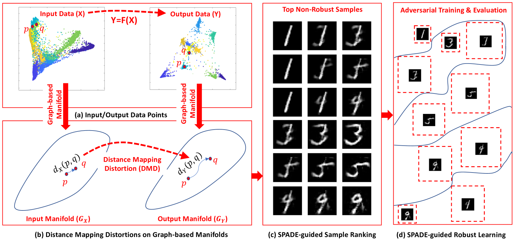
Figure 1: Overview of the proposed method. (a) Given bijective input ($X$) and output ($Y$) data samples, SPADE first constructs graph-based manifolds. (b) SPADE exploits distance mapping distortions (DMDs) on manifolds for adversarial robustness evaluation. (c) Each data sample is given a SPADE score to reflect its level of non-robustness. (d) Applications for SPADE-guided adversarially-robust ML.

Figure 1 shows an overview of SPADE, our spectral method for black-box adversarial robustness evaluation. There are four key steps in our proposed approach: (a) We first construct graph-based manifolds for both input and output data of a given ML model. (b) We then compute the SPADE score for measuring the robustness of the ML model based on bijective distance mapping under the manifold setting. (c) We further extend the SPADE score to quantify the robustness of each input data sample. (d) We also develop SPADE-guided methods for adversarial training and robustness evaluation. As discussed in Section 4, the SPADE-guided adversarial training can be done by adaptively setting the size of the norm-bounded perturbation for each data sample according to its SPADE score, such that stronger defenses can be set up for more vulnerable data samples.

3.1 Graph-based Manifold Construction

In this work, we assume that the input/output data lie near a low-dimensional manifold (Fefferman et al., 2016). We analyze the adversarial robustness of an ML model by transforming its input/output data into a graph, which is a discrete approximation to the underlying manifold. More concretely, consider a given model (e.g., neural networks) that maps a reshaped $M$-dimensional input feature (e.g., image) $x_{i}\in{\mathbb{R}^{M}}$ to a $D$-dimensional output vector $y_{i}\in{\mathbb{R}^{D}}$ through a black-box mapping function $y_{i}=F(x_{i})$. SPADE leverages the k-nearest-neighbor (kNN) algorithm to construct the input (output) graph for input (output) data points, as illustrated by $G_{X}$ ($G_{Y}$) in Figure 1.

Similar to a recent work that exploits graph-based manifolds for the topology analysis of DNNs (Naitzat et al., 2020), we only consider unweighted graphs in this work (namely, each edge has a unit weight). In addition, we choose a proper $k$ value such that the input/output graph is connected. It is worth noting that a naïve implementation of kNN requires $O(|V|^{2})$ time complexity to construct the graph with $O(|V|)$ nodes, which cannot scale to the datasets with millions of data points. Instead, we can leverage an extension of the probabilistic skip list structure to approximate kNN graphs with the complexity of $O(|V|\log|V|)$ (Malkov & Yashunin, 2018).

3.2 The SPADE Score for ML Models

After constructing graph-based manifolds for inputs and outputs, we can analyze the adversarial robustness under the manifold setting through calculating the following metric.

Definition 1.

The distance mapping distortion (DMD) $\gamma^{F}(p,q)$ for a node pair $(p,q)$ through a function $Y=F(X)$ is defined below, where $d_{X}(p,q)$ and $d_{Y}(p,q)$ denote the distances between nodes $p$ and $q$ on the input and output graphs, respectively.

$$\gamma^{F}(p,q)\overset{\mathrm{def}}{=}\frac{d_{Y}(p,q)}{d_{X}(p,q)}$$ (4)

Remark 1.

When $d_{X}(p,q)\to 0$ (i.e., small input perturbation), the DMD metric $\gamma^{F}(p,q)$ can be regarded as a surrogate for the gradient of the function $Y=F(X)$ under the manifold setting.

Intuitively, the maximum DMD ($\gamma^{F}_{max}$) value obtained via exhaustively searching over all node pairs can be exploited for estimating the maximum distance change on the output graph (manifold) due to a small distance perturbation on the input graph (manifold), which therefore allows evaluating the adversarial robustness of a given function (model).

Unlike existing adversarial robustness evaluation methods (e.g., (Szegedy et al., 2013; Goodfellow et al., 2014; Hein & Andriushchenko, 2017; Weng et al., 2018)), the proposed DMD metric for adversarial robustness evaluation does not just target specific types of adversarial attacks or require full access to the underlying model parameters. Instead, our metric can be conveniently obtained by only exploiting input/output data manifolds. In addition, identifying and subsequently correcting the most problematic data samples, the ones that have relatively large DMD values and thus will potentially lead to poor adversarial robustness, will allow training much more adversarially robust models.

3.2.1 Computing $\gamma^{F}_{max}$ via Resistance Distance

Geodesic distance. Pairwise distance calculations on the manifold will be key to estimating $\gamma^{F}_{max}$. To this end, the geodesic distance metric is arguably the most natural choice: for graph-based manifold problems the shortest-path distance metric have been adopted for approximating the geodesic distance on a manifold in nonlinear dimensionality reduction and neural network topological analysis (Tenenbaum et al., 2000; Naitzat et al., 2020). However, to exhaustively search for $\gamma^{F}_{max}$ will require computing all-pairs shortest-paths between $N$ input (output) data points, which can be prohibitively expensive even when taking advantage of the state-of-the-art randomized method (Williams, 2018).

Resistance distance. To avoid staggering computational cost, we propose to compute $\gamma^{F}_{max}$ using effective-resistance distances. Although both geodesic distances and effective-resistances distances are legitimate notions of distances between the nodes on a graph, the latter has been extensively studied in modern spectral graph theory and found close connections to many important problems, such as the cover and commute time of random walks (Chandra et al., 1996), the number of spanning trees of a graph, etc.

Lemma 3.

The effective-resistance distance $d^{\textit{eff}}({p,q})$ between any two nodes $p$ and $q$ for an $N$-node undirected and connected graph $G=(V,E)$ satisfies:

$$d^{\textit{eff}}({p,q})=e_{p,q}^{\top}L_{G}^{+}e_{p,q}=\|U_{N}^{\top}e_{p,q}\|^{2}_{2}$$ (5)

where ${{e_{p,q}=e_{p}-e_{q}}}$, ${{e_{p}\in{\mathbb{R}^{N}}}}$ denotes the standard basis vector with the $p$-th element being $1$ and others being $0$, $L_{G}^{+}\in{\mathbb{R}^{N\times N}}$ denotes the Moore–Penrose pseudoinverse of the graph Laplacian matrix $L_{G}\in{\mathbb{R}^{N\times N}}$, and $U_{N}$ denotes the eigensubspace matrix including $N-1$ nontrivial weighted Laplacian eigenvectors:

$$U_{N}=\left[\frac{u_{2}}{\sqrt{\sigma_{2}}},...,\frac{u_{N}}{\sqrt{\sigma_{N}}}\right]\in{\mathbb{R}^{N\times(N-1)}}$$ (6)

where $0=\sigma_{1}<\sigma_{2},...,\leq\sigma_{N}$ denote the ascending eigenvalues corresponding to their eigenvectors $u_{1},...,u_{N}$.

Lemma 4.

The effective-resistance distance $d^{\textit{eff}}({p,q})$ and geodesic distance $d^{\textit{geo}}({p,q})$ between any two nodes $p$ and $q$ for an $N$-node undirected connected graph satisfies:

1. $d^{\textit{eff}}({p,q})=d^{\textit{geo}}({p,q})$ if there is only one path between nodes $p$ and $q$;

2. $d^{\textit{eff}}({p,q})<d^{\textit{geo}}({p,q})$ otherwise.

Lemma 4 implies that $d^{\textit{eff}}({p,q})=d^{\textit{geo}}({p,q})$ will always be valid for trees, since there will be only one path between any pair of two nodes in a tree. For general graphs, the resistance distance $d^{\textit{eff}}({p,q})$ is bounded by the geodesic distance $d^{\textit{geo}}({p,q})$.

By leveraging resistance distance, we can avoid enumerating all node pairs for calculating $\gamma^{F}_{max}$ by solving the following combinatorial optimization problem:

$$\max{\gamma^{F}}=\mathop{\max_{\forall p,q\in V}}_{p\neq q}\frac{e_{p,q}^{\top}L_{Y}^{+}e_{p,q}}{e_{p,q}^{\top}L_{X}^{+}e_{p,q}}$$ (7)

However, since $e_{p,q}$ is a discrete vector, the above combinatorial optimization problem has a super-linear complexity: approximately finding $\gamma^{F}_{max}$ via computing all-pair effective-resistance distances can be achieved by leveraging Johnson–Lindenstrauss lemma (Spielman & Srivastava, 2011). To avoid the high computational complexity of solving (7), the following SPADE score is proposed for estimating the upper bound of $\gamma^{F}_{max}$, which can be computed in nearly-linear time leveraging recent fast Laplacian solvers (Koutis et al., 2010; Kyng & Sachdeva, 2016).

3.2.2 Estimating $\gamma^{F}_{max}$ via SPADE Score

Definition 2.

Denoting $L_{X}$ ($L_{Y}$) the Laplacian matrix of the input (output) graph $G_{X}$ ($G_{Y}$), the SPADE score of a function (model) $Y=F(X)$ is defined as:

$$\textbf{SPADE}^{F}\overset{\mathrm{def}}{=}\lambda_{max}(L_{Y}^{+}L_{X})$$ (8)

Theorem 1.

When computing $\gamma^{F}_{max}$ via effective-resistance distance, the SPADE score is an upper bound of $\gamma^{F}_{max}$.

The proof for Theorem 1 is available in the Appendix.

Definition 3.

Given two metric spaces $(X,dist_{X})$ and $(Y,dist_{Y})$, where $dist_{X}$ and $dist_{Y}$ denote the distance metrics on the sets $X$ and $Y$, respectively, a function $Y=F(X)$ is called Lipschitz continuous if there exists a real constant $K\geq 0$ such that for all $x_{i}$, $x_{j}\in X$:

$$dist_{Y}(F(x_{i}),F(x_{j}))\leq Kdist_{X}(x_{i},x_{j}),$$ (9)

where $K$ is called the Lipschitz constant for the function $F$. The smallest Lipschitz constant denoted by $K^{*}$ is called the best Lipschitz constant.

Corollary 1.

Let the resistance distance be the distance metric, we have:

$$\lambda_{max}(L_{Y}^{+}L_{X})\geq K^{*}\geq\gamma^{F}_{max}$$ (10)

Corollary 1 indicates that the SPADE score is also an upper bound of the best Lipschitz constant $K^{*}$ under the manifold setting. A greater SPADE score of a function (model) implies a worse adversarial robustness, since the output will be more sensitive to small input perturbations. Thus, we can use the SPADE score to quantify the robustness of a given ML model. We empirically show in Section 5.2 that a more robust model has a smaller SPADE score compared against non-robust models, which confirms the efficacy of our proposed approach.

3.3 The SPADE Score for Input Data Samples

Apart from proposing a metric for evaluating the robustness of machine learning models, we further develop a metric score for revealing the robustness level of each input data sample. Consequently, we can utilize the sample robustness score for ML applications discussed in Section 4.

To measure the robustness per input data sample (i.e., per node), we first measure the robustness of node pairs following the notion of DMD defined in Section 3.2.

Definition 4.

A node pair $(p,q)$ is non-robust if it has a large distance mapping distortion (e.g., $\gamma^{F}(p,q)\approx\gamma^{F}_{max}$).

Intuitively, a non-robust node pair consists of nodes that are adjacent in the input graph $G_{X}$ but far apart in the output graph $G_{Y}$. To effectively reveal the non-robust node pairs, we introduce the cut mapping distortion metric as follows:

Definition 5.

For two graphs $G_{X}$ and $G_{Y}$ that share the same node set $V$, let $S\subset V$ denote a node subset and $\bar{S}$ denote the complement of $S$. Also let $cut_{G}(S,\bar{S})$ denote the number of edges crossing $S$ and $\bar{S}$ in graph $G$. The cut mapping distortion (CMD) $\zeta(S)$ of node subset $S$ is defined as:

$$\zeta(S)\overset{\mathrm{def}}{=}\frac{cut_{G_{Y}}(S,\bar{S})}{cut_{G_{X}}(S,\bar{S})}$$ (11)

A small CMD score indicates that the node pairs crossing the boundary of $S$ are likely to have small distances in $G_{X}$ but rather large distances in $G_{Y}$. As shown in Figure 2, the node subset $S$ has six edges crossing the boundary in $G_{X}$ but only one in $G_{Y}$; as a result, with a high probability the node pairs crossing the boundary will have much smaller effective-resistance or geodesic (shortest-path) distances in $G_{X}$ than $G_{Y}$. For example, nodes $p$ and $q$ are adjacent in $G_{X}$, while they have a large distance in $G_{Y}$ (the shortest-path distance is five).

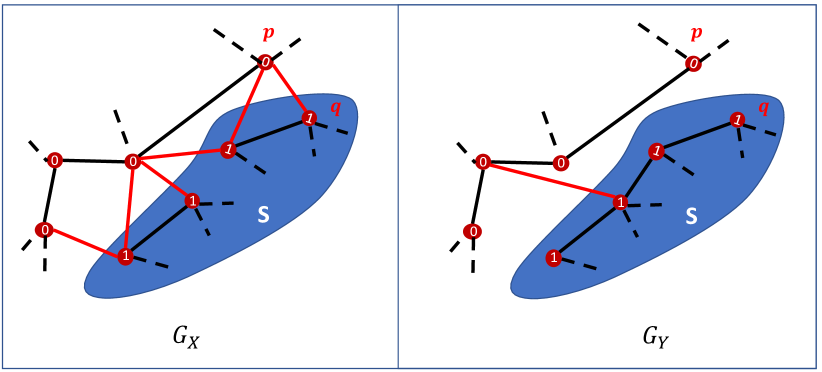
Figure 2: A node coloring vector assigns each node an integer $0$ or $1$ to define the node subset $S$. The cut mapping distortion of $S$ can be computed by: $\zeta(S)=\frac{1}{6}$.

Theorem 2.

Let $L_{X}$ and $L_{Y}$ denote the Laplacian matrices of input and output graphs, respectively. The following inequality holds for the minimum CMD $\zeta_{min}$:

$$\zeta_{min}=\mathop{\min_{\forall S\subset V}}\zeta(S)\geq\frac{1}{\lambda_{max}(L_{Y}^{+}L_{X})}\vspace{-4pt}$$ (12)

The proof is available in the Appendix. Theorem 2 shows the connection between the maximum generalized eigenvalue $\lambda_{max}(L_{Y}^{+}L_{X})$ and $\zeta_{min}$, motivating us to exploit the largest generalized eigenvalues and their corresponding eigenvectors to measure the robustness of node pairs.

Embedding $G_{X}$ with generalized eigenpairs.

Specifically, we first compute the weighted eigensubspace matrix $V_{r}\in{\mathbb{R}^{N\times r}}$ for spectral embedding on $G_{X}$ with $N$ nodes:

$$V_{r}\overset{\mathrm{def}}{=}\left[{v_{1}}{\sqrt{\lambda_{1}}},...,{v_{r}}{\sqrt{\lambda_{r}}}\right],\vspace{-4pt}$$ (13)

where $\lambda_{1},\lambda_{2},...,\lambda_{r}$ represent the first $r$ largest eigenvalues of $L_{Y}^{+}L_{X}$ and $v_{1},v_{2},...,v_{r}$ are the corresponding eigenvectors. To this end, the input graph $G_{X}$ can be embedded using $V_{r}$ such that each node is associated with an $r$-dimensional embedding vector. Subsequently, we can quantify the robustness of an edge $(p,q)\in E_{X}$ via measuring the spectral embedding distance of its two end nodes $p$ and $q$. Formally, we have the following definition:

Definition 6.

The edge SPADE score is defined for any edge $(p,q)\in E_{X}$ as follows:

$$\textbf{SPADE}^{F}(p,q)\overset{\mathrm{def}}{=}\|V_{r}^{\top}e_{p,q}\|_{2}^{2}.\vspace{-10pt}$$ (14)

Theorem 3.

Denote the first $r$ dominant generalized eigenvectors of $L_{X}L_{Y}^{+}$ by $u_{1},u_{2},...,u_{r}$. If an edge $(p,q)$ is dominantly aligned with one dominant eigenvector $u_{k}$, where $1\leq k\leq r$, the following holds:

$$(u^{\top}_{i}e_{p,q})^{2}\approx\begin{cases}\alpha_{k}^{2}\gg 0&\text{ if }(i=k)\\ 0&\text{ if }(i\neq k).\end{cases}\vspace{-5pt}$$ (15)

Then its edge SPADE score has the following connection with its DMD computed using effective-resistance distances:

$$\textbf{SPADE}^{F}(p,q)\propto\left(\gamma^{F}(p,q)\right)^{3}.$$ (16)

The proof is available in the Appendix. So the SPADE score of an edge $(p,q)\in E_{X}$ can be regarded as a surrogate for the directional derivative $\|\nabla_{v}F(x)\|$ under the manifold setting, where $v=\pm(x_{p}-x_{q})$. If an edge has a larger SPADE score, it is considered more non-robust and can be more vulnerable to attacks along the directions formed by its end nodes.

Definition 7.

The node SPADE score is defined for any node (data sample) $p\in V$ as follows:

$$\textbf{SPADE}^{F}(p)\overset{\mathrm{def}}{=}\frac{1}{|\mathbb{N}_{X}(p)|}\sum_{q_{i}\in\mathbb{N}_{X}(p)}{\textbf{SPADE}^{F}(p,q_{i})},\vspace{-4pt}$$ (17)

where $q_{i}\in\mathbb{N}_{X}(p)$ denotes the $i$-th neighbor of node $p$ in graph $G_{X}$, and $\mathbb{N}_{X}(p)\in V$ denotes the node set including all the neighbors of $p$.

The SPADE score of a node (data sample) $p$ can be regarded as a surrogate for the function gradient $\|\nabla F(x)\|$ where $x$ is near $p$ under the manifold setting. A node with a larger SPADE score implies it is likely more vulnerable to adversarial attacks.

4 Applications of SPADE Scores

Model SPADE score. Since the SPADE score of an ML model can be used as a surrogate for the best Lipschitz constant, we can directly use it for quantifying the model’s robustness. A greater SPADE score implies a more vulnerable ML model that can be more easily compromised with adversarial attacks. In practical applications, as long as the input and output data vectors (e.g., $X$ and $Y$) are available, the model SPADE score can be efficiently obtained by constructing the input and output graph-based manifolds (e.g., $G_{X}$ and $G_{Y}$) and subsequently computing the largest generalized eigenvalues using (8). The detailed results are available in Section 5.2.

Node SPADE score. Once we compute the node SPADE score for each input data sample as elaborated in Section 3.3, we can rank all the data samples based on their robustness scores and thus identify the most vulnerable ones, which may benefit the following applications.

4.1 SPADE-Guided Adversarial Training

A recent study shows the following findings (Allen-Zhu & Li, 2020): (1) Training neural networks over the original data is non-robust to small adversarial perturbations, while adversarial training can be provably robust against any small norm-bounded perturbations; (2) The key to improving adversarial robustness is to purify non-robust features that are vulnerable to small, adversarial perturbations along the “dense mixture” directions, via adversarial training; (3) Clean training over the original data will discover a majority of the robust features, while the adversarial training only tries to “purify” some small part of each original feature.

In practice, some data samples may carry greater portions of non-robust features than others, which therefore should be given more attention during adversarial training. To this end, we propose an adaptive, robustness-guided adversarial training scheme by leveraging the SPADE score of each data sample. Specifically, we use a relatively large size of the norm-bounded perturbation (epsilon ball) for data samples with top $k$ highest SPADE score, where $k$ is a hyperparameter. The details about the size of the epsilon ball and $k$ value used in our experiments are available in Section 5.3. This way, much stronger defenses (with large perturbations) towards adversarial attacks should be considered only for the vulnerable data samples with the highest SPADE scores, while normal defenses (with small perturbations) will suffice for the samples with relatively small SPADE scores. The adversarial training results are available in Section 5.3.

4.2 SPADE-Guided Robustness Evaluation

It is worth noting that this application is orthogonal to directly applying the model SPADE score for robustness evaluation. In the latter case, as shown in Theorem 1, the SPADE score is an upper bound of the smallest Lipschitz constant, which is a standalone evaluation metric. In contrast, our goal in this application is to leverage the node SPADE score to identify the most vulnerable data samples, which can guide other metric approaches and facilitate their robustness evaluation of machine learning models. For instance, to evaluate the robustness of a deep neural network using the recent CLEVER method (Weng et al., 2018), a large number of data samples will be randomly selected from the original dataset; then each data sample will be processed for the CLEVER score calculation that may involve many expensive gradient computations. With the guidance of node SPADE score, we only need to check a few of the most non-robust data samples to obtain a reliable CLEVER score, which will greatly improve the computation efficiency when compared with the standard practice. The results of the SPADE-guided CLEVER score are available in Section 5.4.

5 Experimental Results

We conduct four different types of experiments to evaluate the efficacy of our proposed approach. Note that Sections 5.2 and 5.4 exploit the SPADE metric in two orthogonal ways, as explained in Section 4.2.

5.1 Experimental Setup

We obtain the input and output data used in kNN graph construction as shown below.
$\bullet$ MNIST consists of 70,000 images with the size of $28\times 28$. We reshape each image into a $784$ dimensional vector as an input data sample. In addition, we perform inference once on a given pre-trained ML model and extract the $10$ dimensional vector right before the $softmax$ layer per image as the output data sample. Consequently, the input data $X\in{\mathbb{R}^{70,000\times 784}}$ and output data $Y\in{\mathbb{R}^{70,000\times 10}}$ are used to construct the input graph $G_{X}$ and output graph $G_{Y}$, respectively. For the kNN graph construction, we choose $k=10$ ($10\sim 20$) for the training (testing) set.

$\bullet$ CIFAR-10 consists of 60,000 images with the size of $32\times 32\times 3$. We reshape each image into a $3,072$ dimensional vector as an input data sample. Similar to MNIST, we also extract the $10$ dimensional vector right before the $softmax$ layer per image as the output data sample. Subsequently, the input data $X\in{\mathbb{R}^{60,000\times 3,072}}$ and output data $Y\in{\mathbb{R}^{60,000\times 10}}$ are used to construct input graph $G_{X}$ and output graph $G_{Y}$, respectively. We choose $k=100$ ($10\sim 20$) for the training (testing) set in our experiments when constructing the kNN graphs.

5.2 The SPADE Metric for Robustness Evaluation

Model SPADE scores.

To evaluate the model SPADE score as a black-box metric for quantifying model adversarial robustness, for the MNIST and CIFAR-10 test sets we compute the SPADE scores for various models trained with different robustness levels (Madry et al., 2018). For the MNIST dataset, $\epsilon=0.0$ to $0.3$ is considered. For the CIFAR-10 dataset only $\epsilon=0.0$ to $2$ is considered, since for $\epsilon=4$ or $8$ the 10NN/20NN output graphs are not connected. As shown in Table 1, the proposed model SPADE scores consistently reflect the actual levels of model adversarial robustness: in all cases the model SPADE score decreases with the increasing adversarial robustness levels.

Results of DMDs.

Table 2 shows the average DMD values of $100$ edges selected from the input graph $G_{X}$. Here the geodesic distance metric is used for DMD computations, meaning that the DMD value $\gamma^{F}(p,q)$ of each edge $(p,q)$ in $G_{X}$ corresponds to the shortest-path distance between nodes $p$ and $q$ in the output graph $G_{Y}$. The DMD results obtained by selecting the $100$ edges with the largest edge SPADE scores (computed using a single dominant generalized eigenvector) are labeled with “SPADE”, which are compared against the results (labeled with “RANDOM”) of the $100$ edges selected randomly from $G_{X}$. We make the following observations: (1) The edges selected with top SPADE scores have much greater DMDs than those selected randomly, which indicates that SPADE indeed reveals more non-robust node pairs. (2) Another expected yet noteworthy result is that for most cases, the average DMD of randomly selected edges consistently decreases with increasing adversarial robustness levels. This is because more robust models will have a smaller model SPADE scores (upper bound of the best Lipschitz constant) and thus avoid mapping nearby data samples to distant ones. (3) The deeper models (e.g., CIFAR10 models are much deeper than the MNIST ones) map nearby data samples to more distant ones.

Table 1: Model SPADE scores for MNIST ($\epsilon=0.0/0.1/0.2/0.3$) and CIFAR10 ($\epsilon=0.0/0.25/0.5/1.0/2.0$).

Data Set	SPADE (10NN)	SPADE (20NN)
MNIST	$42/40/37/33$	$41/39/36/30$
CIFAR10	$432/256/200/171/79$	$344/195/160/128/61$

Table 2: Average DMDs of $100$ edges in $G_{X}$ for the MNIST ($\epsilon=0.0/0.1/0.2/0.3$) and CIFAR-10 ($\epsilon=0.0/0.25/0.5/1.0/2.0$) data sets. Best results are highlighted.

Test Cases	Avg. DMD (10NN)	Avg. DMD (20NN)
MNIST (SPADE)	6.6/6.1/6.5/7.7	5.1/5.3/5.6/6.4
MNIST (Random)	$3.1/2.6/2.5/2.7$	$2.4/2.3/2.2/2.2$
CIFAR10 (SPADE)	11.4/11.5/9.7/12.5/8.0	8.9/9.0/8.0/10.5/6.8
CIFAR10 (Random)	$6.8/6.4/5.6/5.5/5.3$	$5.7/5.0/4.4/4.3/4.3$

5.3 SPADE-Guided Adversarial Training

Table 3: Classification accuracy under $L_{\infty}$ bounded attacks on MNIST with $\epsilon=0.4$.

Training Methods	Clean	PGD-50	PGD-100	20PGD-100
Vanilla PGD ($\epsilon=0.4$)	$94.38$	$76.89$	$71.45$	$70.23$
PGD-Random ($\epsilon=0.2$&$0.4$)	$\mathbf{97.81}$	$87.89$	$84.22$	$83.09$
PGD-SPADE ($\epsilon=0.2$&$0.4$)	$97.28$	$\mathbf{91.65}$	$\mathbf{89.37}$	$\mathbf{88.46}$

Table 4: Classification accuracy under $L_{\infty}$ bounded attacks on CIFAR-10 with $\epsilon=2.0/4.0/8.0$.

Training Methods	Clean	10PGD-50
Vanilla PGD ($\epsilon=8.0$)	$\mathbf{81.57}$	$75.28/67.92/50.35$
Vanilla PGD ($\epsilon=12.0$)	$76.93$	$71.41/65.58/51.62$
Vanilla PGD ($\epsilon=14.0$)	$75.12$	$70.12/64.64/51.79$
PGD-Random ($\epsilon=12.0$&$14.0$)	$76.09$	$70.87/65.73/51.77$
PGD-SPADE ($\epsilon=12.0$&$14.0$)	$81.38$	$\mathbf{75.74/69.19/53.61}$

Table 5: Comparison of CLEVER scores for robustness evaluation of ML models (Weng et al., 2018). “CNN”, “DD”, and “2CL” stand for the 7-layer AlexNet-like, Defensive Distillation and 2-convolutional-layer CNNs, respectively. The SPADE-guided CLEVER scores are computed using top $10$ (“T10”) non-robust samples and compared against the CLEVER scores computed with $10$ (“R10”) and $100$ (“R100”) randomly selected samples from the MNIST/CIFAR-10 test sets.

Networks	SPADE (10NN,T10)	SPADE (20NN, T20)	CLEVER (R10)	CLEVER (R100)
MNIST-MLP	$1.317/0.067$	$\mathbf{0.590/0.030}$	$0.698/0.034$	$0.819/0.041$
MNIST-CNN	$\mathbf{0.379/0.030}$	$0.391/0.027$	$0.775/0.057$	$0.721/0.057$
MNIST-DD	$\mathbf{0.408/0.026}$	$0.451/0.028$	$0.874/0.065$	$0.865/0.063$
CIFAR-MLP	$\mathbf{0.213/0.004}$	$0.226/0.005$	$0.312/0.007$	$0.219/0.005$
CIFAR-CNN	$0.141/0.004$	$0.088/0.003$	$\mathbf{0.046/0.001}$	$0.072/0.002$
CIFAR-DD	$0.310/0.009$	$0.119/0.003$	$\mathbf{0.100/0.003}$	$0.130/0.004$
MNIST-2CL($\epsilon=0$)	$\mathbf{0.049/0.002}$	$0.075/0.003$	$162.35/7.592$	$68.544/3.182$
MNIST-2CL($\epsilon=0.3$)	$\mathbf{0.112/0.008}$	$0.114/0.006$	$0.332/0.017$	$0.431/0.022$

We choose LeNet-5 and ResNet-18 as basic CNN models on MNIST and CIFAR-10, respectively (LeCun et al., 2015; He et al., 2016). Moreover, we evaluate several baselines as well as our method on MNIST and CIFAR-10 shown below:
$\bullet$ Vanilla PGD. The vanilla projected gradient decent (PGD) based adversarial training approach with perturbation magnitude $\epsilon\in\{0.4\}$ and $\{8.0,12.0,14.0\}$ on MNIST and CIFAR-10, respectively. (Madry et al., 2018).
$\bullet$ PGD-Random. The PGD-based training method but randomly pick $\epsilon$ from $\{0.2,0.4\}$ ($\{12.0,14.0\}$) for each training image on MNIST (CIFAR-10).
$\bullet$PGD-SPADE (Our method). The PGD-based training method with $\epsilon=0.3$ ($14.0$) for top 45,000 non-robust images guided by the node SPADE scores, and $\epsilon=0.3$ ($12.0$) for rest of images on MNIST (CIFAR-10). In addition, to enhance the clean accuracy on CIFAR-10, we skip performing PGD on images that are misclassfied without adversarial perturbation, as suggested in (Balaji et al., 2019; Cheng et al., 2020).

MNIST. We report the averaged classification accuracy over $8$ runs on clean test images as well as perturbed images under $3$ different $L_{\infty}$ bounded attacks with $\epsilon=0.4$: PGD attack with the PGD iteration of 50 (PGD-50) and 100 (PGD-100), and PGD-100 attack with 20 random restarts (20PGD-100) (Madry et al., 2018). All the attacks use $0.01$ step size. As shown in Table 3, our method achieves at least $5.37\%$ accuracy improvement compared against all baselines under the strongest attack (i.e., 20PGD-100). It is worth noting that PGD-SPADE consistently improves the accuracy over PGD-Random under different attacks, which indicates that SPADE can identify the robust images and choose variable epsilon balls accordingly to improve the adversarial accuracy.

CIFAR-10. We report the averaged classification accuracy over $8$ runs on clean as well as perturbed test images under a strong $L_{\infty}$ bounded attack with $\epsilon\in\{2.0,4.0,8.0\}$: PGD attack with 10 random restarts and 50 iterations (i.e., 10PGD-50). All the attacks use a step size of $2.0$. Table 4 shows that our SPADE-guided PGD training method improves the accuracy of PGD-Random as well as the vanilla PGD with all different perturbation magnitudes. This reveals that training with variable epsilon balls guided by the SPADE score indeed enhances the model robustness.

5.4 SPADE-Guided Robustness Evaluation

We choose MNIST and CIFAR-10 for robustness evaluation based on the CLEVER method (Weng et al., 2018). For both datasets, we evaluate CLEVER scores on three networks: a single hidden layer multilayer perceptron (MLP) with the default number of hidden units (Hein & Andriushchenko, 2017), a $7$-layer AlexNet-like CNN with the same structure described in (Carlini & Wagner, 2017), a $7$-layer CNN with defensive distillation (Papernot et al., 2017). For MNIST, we also evaluate CLEVER scores on two $2$-convolutional-layer CNNs (Madry et al., 2018) trained with different robustness levels ($\epsilon=0.0$ and $\epsilon=0.3$). For comparison, we compute the SPADE-guided CLEVER scores for the same datasets using the same networks.

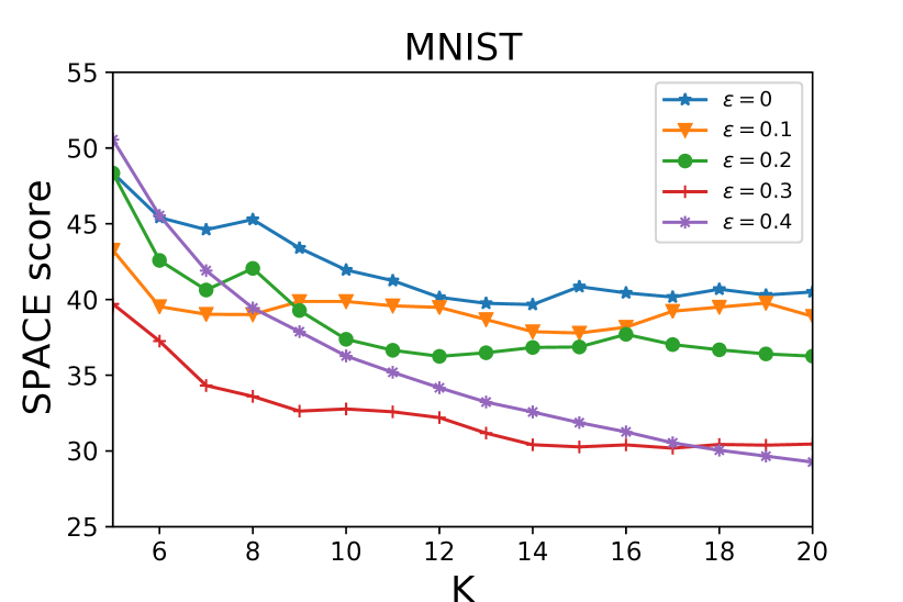
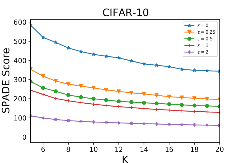
Figure 3: Model SPADE score with varying k values of kNN graph.

For the aforementioned experiments, we use the default sampling parameters in (Weng et al., 2018). Since computing CLEVER score for each image sample can already be time consuming, we only choose $10$ test-set image samples for conducting the untargeted attacks for both MNIST and CIFAR-10. We show the experiment results in Table 5. As expected, in most cases our SPADE-guided CLEVER scores are much smaller than the normal CLEVER scores computed based on randomly selected samples. We also observe that when evaluating CLEVER scores based on a relatively small sample set, the results can be significantly biased. For instance, in the case for MNIST-2CL ($\epsilon=0$), our SPADE-guided score is over $3,000\times$ smaller than the original. Consequently, directly applying CLEVER evaluations without the guidance of SPADE scores may not help correctly assess the model robustness. Here only the SPADE-guided CLEVER scores show consistent robustness evaluations for the MNIST-2CL models trained under $\epsilon=0.0$ and $\epsilon=0.3$ settings.

5.5 Ablation Study on k Value of kNN Graphs

To study the sensitivity of SPADE score to the k value of kNN graph, we use the SPADE score to evaluate non-robustness of models with different k for constructing the kNN graphs. Specifically, we use adversarially trained LeNet5 (ResNet50) model with $\epsilon\in\{0,0.1,0.2,0.3,0.4\}$ ($\epsilon\in\{0,0.25,0.5,1,2\}$) on MNIST (CIFAR-10). The model with higher $\epsilon$ is more adversarially robust. We further vary k from $5$ to $20$ for constructing kNN graphs. As shown in Figure 3, the SPADE scores consistently reveal the model non-robustness on CIFAR-10. For the results on MNIST, SPADE score fails to reflect the model non-robustness (e.g., the model with $\epsilon=0.4$) when k is too small ($k<10$). However, the SPADE score gradually captures model non-robustness when increasing the k value and correctly ranks the non-robustness of all models with $k=20$. Thus, a relatively large k (e.g., $20$) is preferred when constructing kNN graphs for computing the SPADE score.

6 Conclusion

This work introduces SPADE, a black-box spectral method for evaluating the adversarial robustness of a given ML model based on graph-based manifolds. We formally prove that the proposed SPADE metric is an upper bound of the best Lipschitz constant under the manifold setting. Moreover, we extend the SPADE score to identify the most non-robust data samples that are potentially vulnerable to adversarial perturbations. Our extensive experiments show that the model SPADE score is a good surrogate for the best Lipschitz constant, and thus can be leveraged for revealing the level of adversarial robustness of a given ML model. In addition, our results show that the sample SPADE scores can be exploited for enhancing the performance of existing adversarial training as well as adversarial robustness evaluations.

7 Acknowledgments

This work is supported in part by the National Science Foundation under Grants CCF-2041519, CCF-2021309, CCF-2011412, and CCF-2007832. The authors would like to thank Weizhe Hua (Cornell) and Shusen Wang (Stevens) for their helpful discussions on the topic of adversarial training.

Appendix A Supplementary Materials

A.1 Proof for Theorem $\mathbf{1}$

Proof.

We first compute effective-resistance distance between nodes $p$ and $q$ on $G_{Y}$ and $G_{X}$ by $d_{Y}(p,q)=e_{p,q}^{\top}L_{Y}^{+}e_{p,q}$ and $d_{X}(p,q)=e_{p,q}^{\top}L_{X}^{+}e_{p,q}$, respectively. Consequently, $\gamma^{F}_{max}$ satisfies the following inequality:

$$\gamma^{F}_{max}=\mathop{\max_{\forall p,q\in V}}_{p\neq q}\frac{e_{p,q}^{\top}L_{Y}^{+}e_{p,q}}{e_{p,q}^{\top}L_{X}^{+}e_{p,q}}\leq\mathop{\max_{||{v}||\neq 0}}_{v^{\top}\mathbf{1}=0}\frac{v^{\top}L_{Y}^{+}v}{v^{\top}L_{X}^{+}v}$$ (18)

where $\mathbf{1}\in{\mathbb{R}^{N}}$ denotes the all-one vector. According to the generalized Courant-Fischer theorem, we have:

$$\mathop{\max_{||{v}||\neq 0}}_{v^{\top}\mathbf{1}=0}\frac{v^{\top}L_{Y}^{+}v}{v^{\top}L_{X}^{+}v}=\lambda_{max}(L_{X}L_{Y}^{+})=\lambda_{max}(L_{Y}^{+}L_{X})$$ (19)

By combining Equations (18) and (19), we have:

$$\gamma^{F}_{max}\leq\mathop{\max_{||{v}||\neq 0}}_{v^{\top}\mathbf{1}=0}\frac{v^{\top}L_{X}v}{v^{\top}L_{Y}v}=\lambda_{max}(L_{Y}^{+}L_{X})$$ (20)

which completes the proof of the theorem. ∎

A.2 Proof for Theorem $\mathbf{2}$

Proof.

Before proving our theorem, we first introduce the formal definition of node subset and its boundary in a graph:

Definition 8.

Given a node coloring vector $z\in{\mathbb{R}^{N}}$ including only $0$s and $1$s, a node subset $S_{z}\subset V$ and its complement $\overline{S}_{z}\subset V$ are defined as follows, respectively:

$$\begin{split}S_{z}\overset{\mathrm{def}}{=}\left\{p\in V:z(p)=1\right\},\\ \overline{S}_{z}\overset{\mathrm{def}}{=}\left\{p\in V:z(p)=0\right\}.\end{split}$$ (21)

Definition 9.

The boundaries $\partial_{G_{X}}(S_{z})$ and $\partial_{G_{Y}}(S_{z})$ of $S_{z}$ in graphs $G_{X}$ and $G_{Y}$ are defined as follows, respectively:

$$\begin{split}\partial_{G_{X}}(S_{z})\overset{\mathrm{def}}{=}\left\{(p,q)\in E_{X}:p\notin S_{z},q\in S_{z}\right\},\\ \partial_{G_{Y}}(S_{z})\overset{\mathrm{def}}{=}\left\{(p,q)\in E_{Y}:p\notin S_{z},q\in S_{z}\right\}.\end{split}$$ (22)

Consequently, the cut (the size of the boundary) of $S_{z}$ in each of $G_{X}$ and $G_{Y}$ can be computed as follows, respectively:

$$\begin{split}cut_{X}(S_{z},\overline{S}_{z})&={z}^{\top}{L}_{X}{z}=|\partial_{G_{X}}(S_{z})|,\\ cut_{Y}(S_{z},\overline{S}_{z})&={z}^{\top}{L}_{Y}{z}=|\partial_{G_{Y}}(S_{z})|.\end{split}$$ (23)

According to the generalized Courant-Fischer theorem, we have the following inequality:

$$\lambda_{max}(L_{Y}^{+}L_{X}) =\mathop{\max_{|{v}|\neq 0}}_{v^{\top}\mathbf{1}=0}\frac{v^{\top}L_{X}v}{v^{\top}L_{Y}v}$$

$$\geq\mathop{\max_{\forall S_{z}\subset V}}\frac{{z}^{\top}{L}_{X}{z}}{{z}^{\top}{L}_{Y}{z}}$$

$$=\mathop{\max_{\forall S_{z}\subset V}}\frac{|\partial_{G_{X}}(S_{z})|}{|\partial_{G_{Y}}(S_{z})|}$$

$$=\frac{1}{\zeta^{F}_{min}}$$

which completes the proof of the theorem. ∎

A.3 Proof for Theorem $\mathbf{3}$

Proof.

Let $u_{1},u_{2},...,u_{N}$ and $v_{1},v_{2},...,v_{N}$ denote the $N$ eigenvectors of $L_{X}L_{Y}^{+}$ and $L_{Y}^{+}L_{X}$, respectively, while their corresponding shared eigenvalues are denoted by $\lambda_{1},\lambda_{2},...,\lambda_{N}$. In addition, eigenvectors ${{u_{i}}}$ can be constructed to satisfy:

$${u_{i}^{\top}L^{+}_{X}u_{j}}=\left\{\begin{array}[]{l}1,~{}~{}~{}i=j\\ 0,~{}~{}~{}i\neq j.\end{array}\right.$$ (24)

$$\Rightarrow{u_{i}^{\top}L^{+}_{Y}u_{j}}=\left\{\begin{array}[]{l}\lambda_{i},~{}~{}~{}i=j\\ 0,~{}~{}~{}i\neq j.\end{array}\right.$$ (25)

Therefore, the following equations hold:

$$\begin{split}L_{Y}^{+}u_{i}&=\lambda_{i}L_{X}^{+}u_{i}\leftrightarrow L_{Y}^{+}L_{X}\left(L_{Y}^{+}u_{i}\right)=\lambda_{i}\left(L_{Y}^{+}u_{i}\right)\\ L_{X}v_{i}&=\lambda_{i}L_{Y}v_{i}\leftrightarrow L_{Y}^{+}L_{X}v_{i}=\lambda_{i}v_{i}\end{split}$$ (26)

which leads to the following equation

$$\begin{split}v_{i}&=\beta_{i}L_{Y}^{+}u_{i}\\ \Rightarrow u^{\top}_{j}v_{i}&=\left\{\begin{array}[]{l}\beta_{i}\lambda_{i},~{}~{}~{}i=j\\ 0,~{}~{}~{}i\neq j.\end{array}\right.\end{split}$$ (27)

where $\beta_{i}$ denotes a scaling coefficient. Without loss of generality, $e_{p,q}$ can be expressed as a linear combination of $u_{i}$ for $i=1,...,N$ as follows:

$$e_{p,q}=\sum_{i=1}^{N}\alpha_{i}u_{i}.$$ (28)

Then $\gamma^{F}(p,q)$ can be rewritten as follows:

$$\begin{split}\gamma^{F}(p,q)&=\frac{d_{Y}(p,q)}{d_{X}(p,q)}=\frac{e_{p,q}^{\top}L_{Y}^{+}e_{p,q}}{e_{p,q}^{\top}L_{X}^{+}e_{p,q}}\\ &=\frac{(\sum_{i=1}^{N}\alpha_{i}u_{i})^{\top}L_{Y}^{+}(\sum_{i=1}^{N}\alpha_{i}u_{i})}{(\sum_{i=1}^{N}\alpha_{i}u_{i})^{\top}L_{X}^{+}(\sum_{i=1}^{N}\alpha_{i}u_{i})}\\ &=\frac{\sum_{i=1}^{N}\sum_{j=1}^{N}\alpha_{i}\alpha_{j}u_{i}^{\top}L_{Y}^{+}u_{j}}{\sum_{i=1}^{N}\sum_{j=1}^{N}\alpha_{i}\alpha_{j}u_{i}^{\top}L_{X}^{+}u_{j}}\\ &=\frac{\sum_{i=1}^{N}\alpha^{2}_{i}u_{i}^{\top}L_{Y}^{+}u_{i}}{\sum_{i=1}^{N}\alpha^{2}_{i}u_{i}^{\top}L_{X}^{+}u_{i}}\\ &=\frac{\sum_{i=1}^{N}\alpha^{2}_{i}\lambda_{i}}{\sum_{i=1}^{N}\alpha^{2}_{i}}.\end{split}$$ (29)

If the edge $({p,q})$ is dominantly aligned with a single dominant generalized eigenvector $u_{k}$ where $1\leq k\leq r$, it implies $\forall i\neq k,\alpha_{i}\approx 0$ and thus $e_{p,q}\approx\alpha_{k}u_{k}$. Then $\gamma^{F}(p,q)$ can be approximated by:

$$\begin{split}\gamma^{F}(p,q)\approx\lambda_{k}.\end{split}$$ (30)

On the other hand, (27) allows the edge SPADE score of $({p,q})$ to be expressed as

$$\begin{split}\textbf{SPADE}^{F}(p,q)&=\|V_{r}^{\top}e_{p,q}\|_{2}^{2}\\ &=\sum_{i=1}^{r}\lambda_{i}(v_{i}^{\top}e_{p,q})^{2}\\ &=\sum_{i=1}^{r}\lambda_{i}\left(\sum_{j=1}^{N}\alpha_{j}\beta_{i}u_{j}^{\top}L_{Y}^{+}u_{i}\right)^{2}\\ &=\sum_{i=1}^{r}\alpha^{2}_{i}\beta^{2}_{i}\lambda^{3}_{i}\\ &\approx\alpha^{2}_{k}\beta^{2}_{k}\lambda^{3}_{k}\propto\left(\gamma^{F}(p,q)\right)^{3}\end{split}$$ (31)

which completes the proof of the theorem. ∎

A.4 A Spectral Perspective of Adversarial Training

The Riemannian distance between positive definite (PSD) matrices has been considered as the most natural and useful distance defined on the positive definite cone $\mathbb{S}^{n}_{++}$ (Bonnabel & Sepulchre, 2010).

Definition 10.

The Riemannian distance $\delta({L_{X}},{L_{Y}})$ between $L_{X}$ and $L_{Y}$ is given by (Lim et al., 2019):

$$\delta({L_{Y}},{L_{X}})=\delta({L_{X}},{L_{Y}})\overset{\mathrm{def}}{=}\left[\sum_{i=1}^{N}\log^{2}\lambda_{i}(L_{Y}^{+}L_{X})\right]^{\frac{1}{2}}.$$ (32)

The Riemannian distance $\delta({L_{X}},{L_{Y}})$ requires all eigenvalues of $L_{Y}^{+}L_{X}$ to be evaluated, and therefore encapsulates all possible cut mapping distortions.

While $\lambda_{max}(L_{Y}^{+}L_{X})$ tells if function $F$ can map two nearby data points (nodes) to distant ones at output, $\lambda_{max}(L_{X}^{+}L_{Y})$ tells if there exist two neighboring output data points (nodes) that are mapped from two distant ones at input. Since $\lambda_{max}(L_{Y}^{+}L_{X})\gg\lambda_{max}(L_{X}^{+}L_{Y})$ holds for most machine learning applications, $\lambda_{max}(L_{Y}^{+}L_{X})$ will be more interesting and relevant to adversarial robustness.

Remark 2.

The Riemannian distance $\delta({L_{Y}},{L_{X}})$ for a typical ML model will be upper bounded by:

$$\begin{split}\delta({L_{Y}},{L_{X}})\leq N\log\lambda_{max}(L_{Y}^{+}L_{X}).\end{split}$$ (33)

Definition 11.

Given two metric spaces $(X,dist_{X})$ and $(Y,dist_{Y})$, where $dist_{X}$ and $dist_{Y}$ denote the metrics on the sets $X$ and $Y$ respectively, if there exists a $\kappa\geq 1$ with:

$$\frac{1}{\kappa}dist_{X}(p,q)\leq dist_{Y}(p,q)\leq\kappa dist_{X}(p,q),$$ (34)

then $Y=F(X)$ is called a $\kappa$-bi-Lipschitz mapping, which is injective, and is a homeomorphism onto its image.

Choosing $\kappa=\lambda_{max}(L_{Y}^{+}L_{X})=\textbf{SPADE}^{F}$ will make $Y=F(X)$ a $\kappa$-bi-Lipschitz mapping under the manifold setting.

Remark 3.

Adversarial training can effectively decrease the Riemannian distances between the input and output manifolds, which is similar to decreasing the Lipschitz constant.

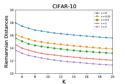
Figure 4: Riemannian distances of adversarially-trained models. A greater $\epsilon$ value indicates a more adversarially robust NN model.

An example. We demonstrate the Riemannian distances of the PGD trained neural networks in Figure 4. Our results are obtained using the CIFAR-10 data set, which includes $10,000$ images (data points). We construct $k$-nearest-neighbor (kNN) graphs for approximating the input/output data manifolds with varying $k$ values. The Riemannian distances have been calculated only using the $10$ largest eigenvalues of $L_{Y}^{+}L_{X}$. As shown in Figure 4, the more adversarially robust neural networks always exhibit lower Riemannian distances.

A.5 Eigensolver for computing SPADE score

Table 6: Eigensolver performance when using eigs and power iteration method for MNIST and CIFAR-10 data sets with $\epsilon=0$.

	MNIST		CIFAR-10
	eigs	power_iteration	eigs	power_iteration
$K=10$, $\lambda_{max}(L_{Y}^{+}L_{X})$	98.64	98.38 (err = 0.26%)	398.16	396.48 (err = 0.42%)
$K=10$, runtime	9.22s	5.88s	11.96s	2.65s
$K=20$, $\lambda_{max}(L_{Y}^{+}L_{X})$	81.14	80.83 (err = 0.38%)	311.49	310.21 (err = 0.41%)
$K=20$, runtime	16.19s	7.62s	19.40s	7.29s

To efficiently find the SPADE score, power iteration method can be leveraged to compute the dominant eigenvalues of $L_{Y}^{+}L_{X}$. To further reduce the complexity, graph-theoretic algebraic multigrid solvers (Koutis et al., 2011; Livne & Brandt, 2012) can be applied to solve the corresponding graph Laplacians. To evaluate the performance of the power iteration method, we calculated the largest eigenvalue of $L_{Y}^{+}L_{X}$ using built-in MATLAB eigs function and the power iteration method, where $L_{X}$ and $L_{Y}$ represent the kNN graph Laplacians constructed based on MNIST and CIFAR-10 dataset with K being 10 and 20. As shown in Table 6, $\lambda_{max}(L_{Y}^{+}L_{X})$ and the corresponding run time are reported in the table under different settings; ERR represents the relative error of $\lambda_{max}(L_{Y}^{+}L_{X})$ comparing with eigs. From the table we observe that power iteration method allows efficiently computing $\lambda_{max}(L_{Y}^{+}L_{X})$ with satisfactory accuracy levels.

A.6 Spectral Embedding and SPADE Scores

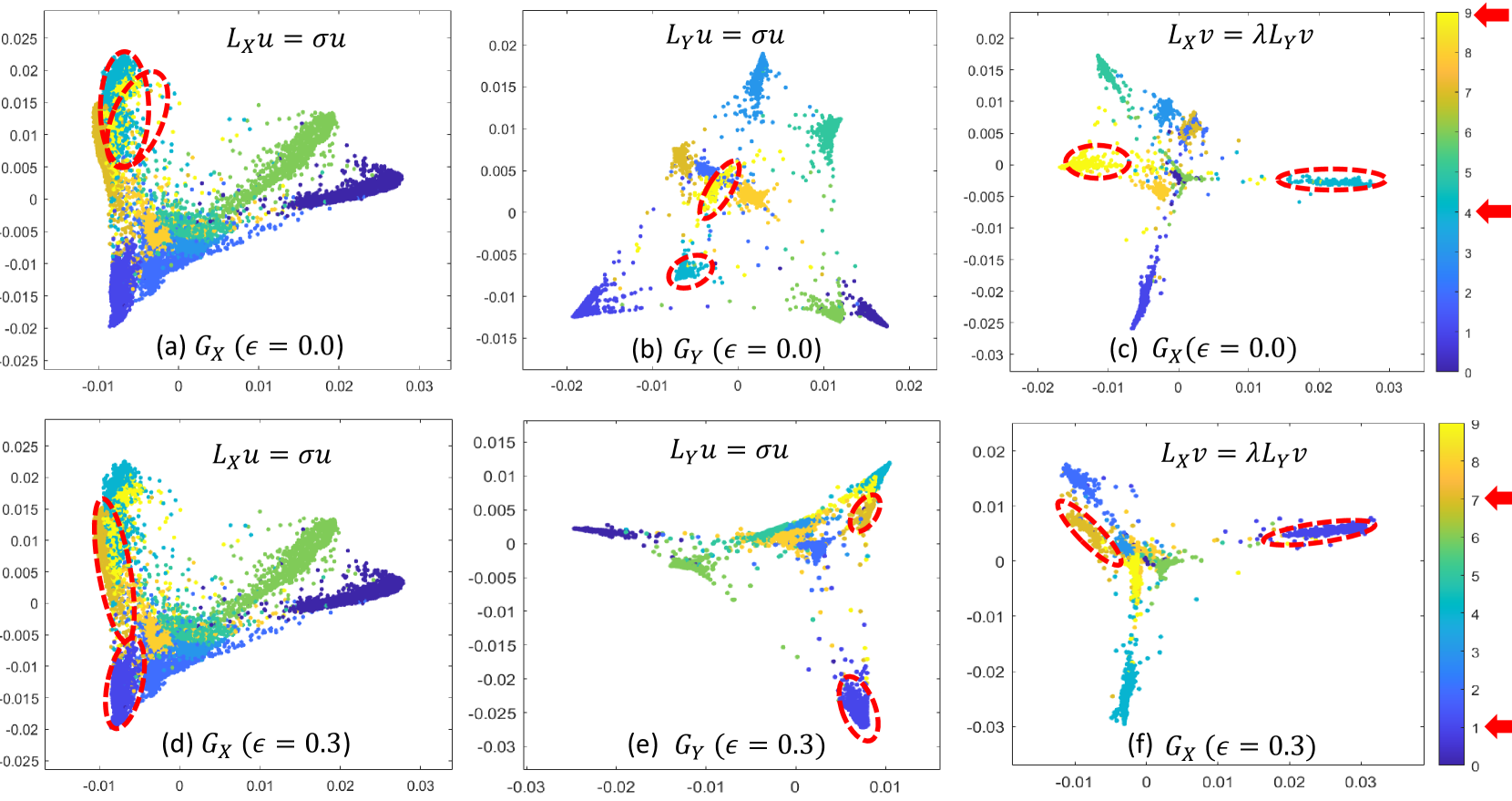
Figure 5: Revealing non-robust node pairs via spectral embedding w/ the first two Laplacian and generalized eigenvectors before (top row) and after (bottom row) adversarial training. The labels of the most non-robust node pairs are indicated by red arrows for both settings.

Figure 5 shows the 2D spectral node embeddings before/after adversarial training with the first two eigenvectors of $L_{X}$, $L_{Y}$ and $L^{+}_{Y}L_{X}$, respectively, for the MNIST test set that includes $10,000$ handwritten digits from $0$ to $9$. The edges are not shown for the sake of clarity. The following has been observed: (1) Before adversarial training, the handwritten digits of $4$ and $9$ are very close at input but much more separated at output as shown in Figures (a) and (b), which implies a rather poor adversarial robustness level; a similar conclusion can be made by checking the node embedding with generalized eigenvectors in Figure (c), where $4$ and $9$ clusters are most separated from each other. (2) After adversarial training, the $4$ and $9$ clusters are much closer at output as shown in Figure (e), which is due to the substantially improved robustness, while digits $1$ and $7$ become the most non-robust ones as shown in Figure (f).

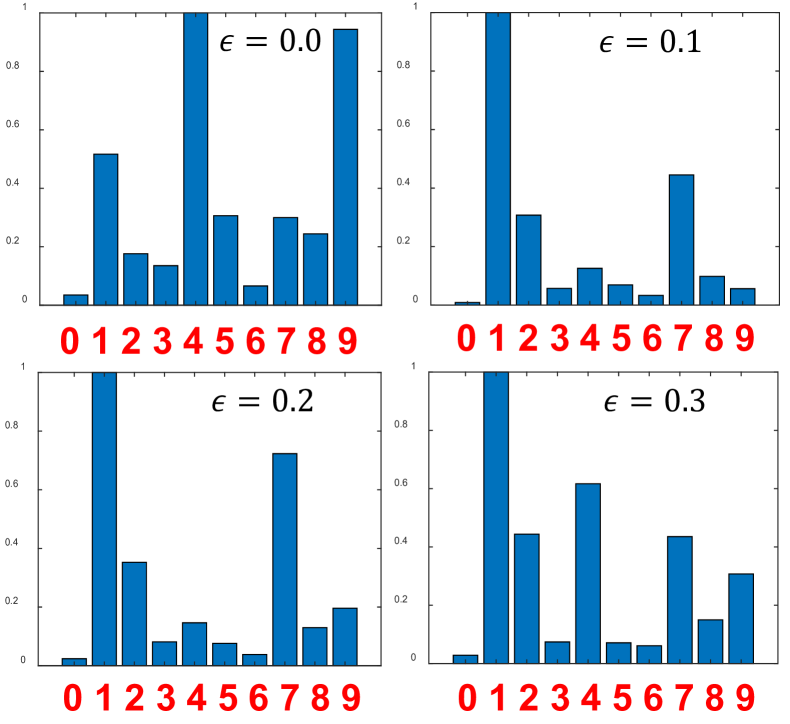
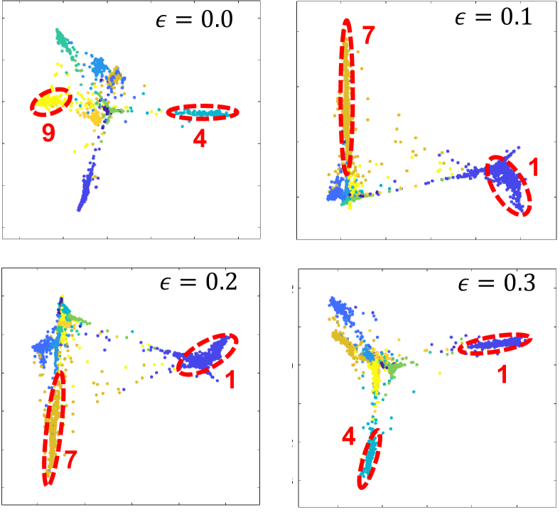
Figure 6: The label SPADE scores and spectral embeddings with top two dominant generalized eigenvectors (MNIST test set).

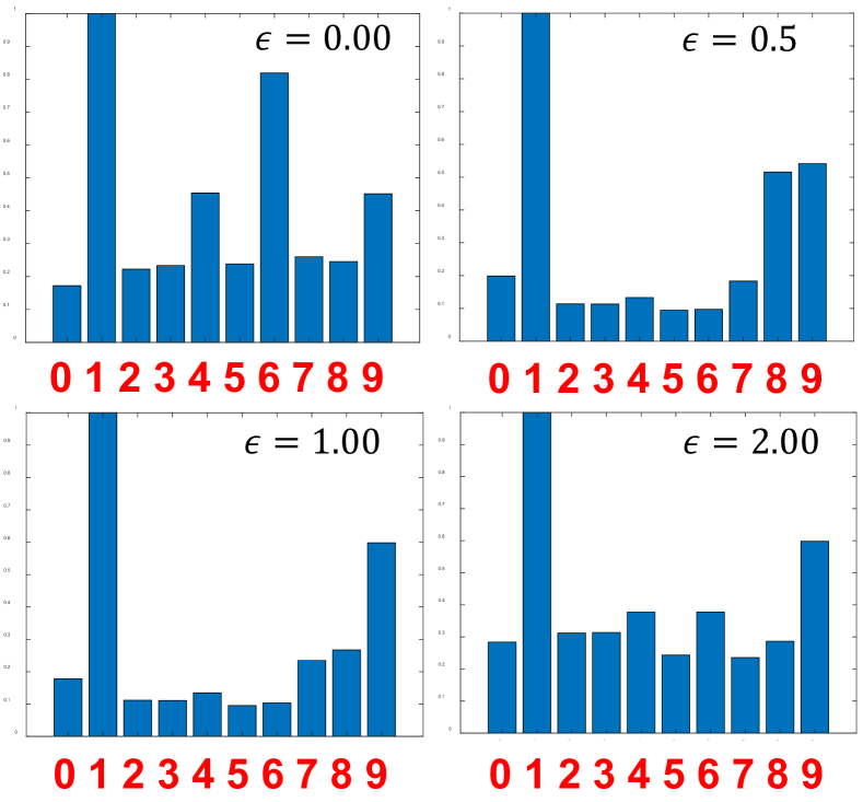
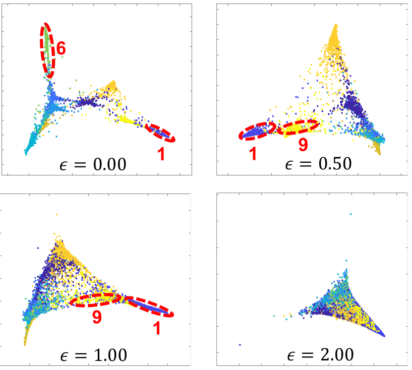
Figure 7: The label SPADE scores and spectral embeddings with top two dominant generalized eigenvectors (CIFAR-10 test set).

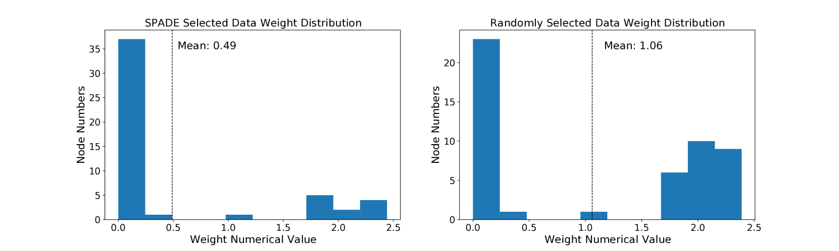
Figure 8: The GAIRAT weight distributions of 50 SPADE-guided (left) and randomly selected (right) data samples

Figures 6 and 7 show the SPADE scores of each label under four different adversarial robustness levels for the MNIST and CIFAR-10 test sets, where the corresponding 2D spectral embeddings using dominant generalized eigenvectors are also demonstrated. It is observed that for the clean models ($\epsilon=0$), labels $4$ and $9$ ($1$ and $6$) are the most vulnerable labels for MNIST (CIFAR-10). After adversarial training with different adversarial robustness levels, labels $1$ and $7$ remain the most vulnerable ones for MNIST, while labels $1$ (automobile) and $9$ (truck) remain the most vulnerable ones for CIFAR-10. It is also observed in both test cases that the spectral embeddings become less scattered for more adversarial robust models. As shown in Figure 7, the spectral embedding of the most robust model trained with $\epsilon=2$ only forms a single cluster, implying indistinguishable vulnerabilities across different labels.

A.7 SPADE for Topology Analysis of Neural Networks

Figure 9 shows the SPADE scores computed using the output data associated with different layers of a neural network model trained on the point cloud datasets D-I and D-II (Naitzat et al., 2020), which implies that deeper architectures will result in greater Lipschitz constant and thus SPADE scores. Such results also allows analyzing the topology changes across different neural network layers. For instance, it is observed that the sharply decreasing Betti numbers for the neural network layers $4$ to $7$ of the D-II data set correspond to dramatically increasing SPADE scores.

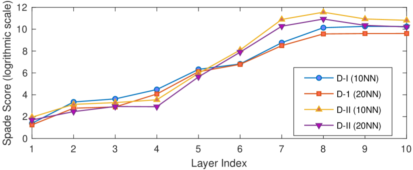
Figure 9: The layer-wise SPADE scores of neural network models

A.8 Model SPADE Score for the CINIC-$10$ dataset

Table 7: Model SPADE scores for the CINIC-10 dataset (Darlow et al., 2018)

CINIC	SPADE(10NN)	SPADE(20NN)	SPADE(50NN)	SPADE(100NN)
$\epsilon=0$	$648.64$	$1393.71$	$263.69$	$214.01$
$\epsilon=0.25$	$348.45$	$267.77$	$201.33$	$164.30$
$\epsilon=0.5$	$285.68$	$219.91$	$166.53$	$135.66$
$\epsilon=1.0$	$274.17$	$210.18$	$156.00$	$124.55$

Apart from MNIST and CIFAR-$10$ data sets, we further compute the SPADE scores on the CINIC-$10$ dataset (Darlow et al., 2018), which is larger version of CIFAR-$10$ and its test set contains $90,000$ images (data points). The result is demonstrated in Table 7. Similar to the results of MNIST and CIFAR-$10$ data sets, the more robust neural networks always reveal lower SPADE scores.

A.9 Model SPADE Score for Natural Robustness

Table 8: Model SPADE scores for four networks trained with standard CIFAR-10 data and AugMix processed CIFAR-10 data. We evaluate SPADE scores on both clean test set and corrupted test set via data shift.

Networks	AugMix (Clean)	Standard (Clean)	AugMix (Corrupted)	Standard (Corrupted)
Allconv	$149.63$	$213.03$	$60.68$	$39.99$
Densenet	$129.49$	$152.07$	$53.32$	$33.63$
Resnext	$571.15$	$614.63$	$293.94$	$51.57$
WRN	$738.35$	$784.03$	$100.17$	$72.96$

(Hendrycks et al., 2019) proposes a data processing technique called AugMix, which enhances the natural robustness of various CNN architectures to data shift. In this experiment, we compute SPADE scores for both standard models and AugMix trained models. As demonstrated in Table8, the more robust (AugMix-trained) models always have lower SPADE scores on the clean test set, but greater SPADE scores for the corrupted data set generated via adding various noises (Hendrycks & Dietterich, 2019).

A.10 Comparison of Graph Construction Methods

Table 9: Comparison of model CLEVER scores on MNIST/CIFAR-10 test sets (Weng et al., 2018). CNN, DD, and 2CL represent the 7-layer AlexNet-like, Defensive Distillation, and 2-convolutional-layer CNNs. GRASS (Feng, 2020), PCA, CKNN, and KNN stand for different graph-based manifold constructions. “T10” (“B10”) denote the SPADE-guided CLEVER scores computed via sampling the top (bottom) $10$ most non-robust samples, respectively, based on node SPADE score.

Networks	GRASS (10NN, T10)	GRASS (10NN, B10)	PCA (10NN, T10)	PCA (10NN, B10)
MNIST-2CL($\epsilon=0$)	$0.964/0.0465$	$21.136/0.985$	$0.195/0.011$	$21.742/1.078$
MNIST-2CL($\epsilon=0.3$)	$0.045/0.006$	$5.574/0.623$	$0.034/0.005$	$7.750/0.971$
MNIST-MLP	$0.432/0.020$	$1.729/0.089$	$0.460/0.022$	$1.564/0.079$
MNIST-CNN	$0.570/0.044$	$0.983/0.083$	$0.525/0.040$	$1.099/0.099$
MNIST-DD	$0.448/0.028$	$1.306/0.094$	$0.377/0.027$	$1.487/0.101$
CIFAR-MLP	$0.113/0.002$	$0.253/0.005$	$0.535/0.012$	$0.214/0.004$
CIFAR-CNN	$0.230/0.007$	$0.167/0.004$	$0.214/0.006$	$0.114/0.003$
CIFAR-DD	$0.287/0.009$	$0.111/0.003$	$0.245/0.008$	$0.167/0.005$
Networks	CKNN (10NN, T10)	CKNN (10NN, B10)	KNN (10NN, T10)	KNN (10NN, B10)
MNIST-2CL($\epsilon=0$)	$0.784/0.039$	$0.801/0.040$	$0.049/0.002$	$20.499/0.950$
MNIST-2CL($\epsilon=0.3$)	$0.541/0.049$	$0.712/0.072$	$0.112/0.008$	$4.888/0.620$
MNIST-MLP	$0.555/0.039$	$0.850/0.058$	$1.317/0.067$	$1.715/0.089$
MNIST-CNN	$0.070/0.001$	$0.204/0.004$	$0.379/0.030$	$0.894/0.079$
MNIST-DD	$0.045/0.001$	$0.100/0.002$	$0.408/0.026$	$1.399/0.097$
CIFAR-MLP	$0.078/0.002$	$0.129/0.004$	$0.213/0.004$	$0.253/0.005$
CIFAR-CNN	$0.185/0.009$	$8.938/0.423$	$0.141/0.004$	$0.215/0.006$
CIFAR-DD	$0.434/0.048$	$0.075/0.003$	$0.318/0.036$	$0.111/0.003$

This set of experiments examine how graph construction methods would impact the computation of SPADE scores. To this end, we have tested the following four methods for constructing the graph-based manifolds: 1. GRASS: The vanilla kNN graph with spectral sparsification (Feng, 2020); 2. PCA: The vanilla kNN graph constructed after mapping the original data samples to lower dimensional space via principal component analysis (PCA) (Jolliffe & Cadima, 2016); 3. CKNN: The kNN graph constructed using continuous k-nearest neighbors (CKNN) (Berry & Sauer, 2016); 4. KNN: The vanilla k-nearest neighbor graph.

We apply the above graph construction methods and compute the sample SPADE scores accordingly. Then $10$ most non-robust (top) and robust (bottom) samples are used for computing the CLEVER scores. Since the CLEVER score is the lower bound on the minimal distortion to obtaining adversarial samples (Weng et al., 2018), we expect that the CLEVER score computed by robust samples should be greater than that computed by non-robust samples. As shown in Table 9, all four graph construction methods obtain a larger CLEVER score for B10 than T10 for most models. However, the gap between CLEVER scores of T10 and B10 varies from different graphs and models. For instance, the CKNN-based CLEVER score has a relatively smaller gap between T10 and B10 than other methods for the MNIST-2CL model, while it has a larger gap than other methods for the CIFAR-CNN model.

A.11 Correlation between SPADE and GAIRAT

(Zhang et al., 2021) introduces a white-box measurement of data robustness called GAIRAT, which adopts the idea that a data sample closer to the decision boundary is less robust. Consequently, GAIRAT assigns smaller weights on training losses to data samples that are farther from the decision boundary. To verify that our node SPADE score indeed captures the robustness of data samples, we compare the weights of the top $50$ most robust samples (with the lowest SPADE scores) with the weights of $50$ randomly selected samples. As observed in Figure 8, the SPADE-guided samples have much smaller weights than the randomly selected samples, which implies the node SPADE scores can be leveraged for effectively identifying the most robust samples.

References

- Allen-Zhu & Li (2020) Allen-Zhu, Z. and Li, Y. Feature purification: How adversarial training performs robust deep learning. arXiv preprint arXiv:2005.10190, 2020.
- Balaji et al. (2019) Balaji, Y., Goldstein, T., and Hoffman, J. Instance adaptive adversarial training: Improved accuracy tradeoffs in neural nets. arXiv preprint arXiv:1910.08051, 2019.
- Barreno et al. (2010) Barreno, M., Nelson, B., Joseph, A. D., and Tygar, J. D. The security of machine learning. Machine Learning, 81(2):121–148, 2010.
- Berry & Sauer (2016) Berry, T. and Sauer, T. Consistent manifold representation for topological data analysis. arXiv preprint arXiv:1606.02353, 2016.
- Biggio et al. (2013) Biggio, B., Fumera, G., and Roli, F. Security evaluation of pattern classifiers under attack. IEEE Transactions on Knowledge and Data Engineering, 26(4):984–996, 2013.
- Bonnabel & Sepulchre (2010) Bonnabel, S. and Sepulchre, R. Riemannian metric and geometric mean for positive semidefinite matrices of fixed rank. SIAM Journal on Matrix Analysis and Applications, 31(3):1055–1070, 2010.
- Carlini & Wagner (2017) Carlini, N. and Wagner, D. Towards evaluating the robustness of neural networks. In 2017 IEEE Symposium on Security and Privacy (SP), pp. 39–57. IEEE, 2017.
- Chandra et al. (1996) Chandra, A. K., Raghavan, P., Ruzzo, W. L., Smolensky, R., and Tiwari, P. The electrical resistance of a graph captures its commute and cover times. Computational Complexity, 6(4):312–340, 1996.
- Cheng et al. (2020) Cheng, M., Lei, Q., Chen, P.-Y., Dhillon, I., and Hsieh, C.-J. Cat: Customized adversarial training for improved robustness. arXiv preprint arXiv:2002.06789, 2020.
- Cisse et al. (2017) Cisse, M., Bojanowski, P., Grave, E., Dauphin, Y., and Usunier, N. Parseval networks: Improving robustness to adversarial examples. In International Conference on Machine Learning, pp. 854–863. PMLR, 2017.
- Darlow et al. (2018) Darlow, L. N., Crowley, E. J., Antoniou, A., and Storkey, A. J. Cinic-10 is not imagenet or cifar-10. arXiv preprint arXiv:1810.03505, 2018.
- Fawzi et al. (2018) Fawzi, A., Fawzi, O., and Frossard, P. Analysis of classifiers’ robustness to adversarial perturbations. Machine Learning, 107(3):481–508, 2018.
- Fefferman et al. (2016) Fefferman, C., Mitter, S., and Narayanan, H. Testing the manifold hypothesis. Journal of the American Mathematical Society, 29(4):983–1049, 2016.
- Feinman et al. (2017) Feinman, R., Curtin, R. R., Shintre, S., and Gardner, A. B. Detecting adversarial samples from artifacts. arXiv preprint arXiv:1703.00410, 2017.
- Feng et al. (2019) Feng, F., He, X., Tang, J., and Chua, T.-S. Graph adversarial training: Dynamically regularizing based on graph structure. IEEE Transactions on Knowledge and Data Engineering, 2019.
- Feng (2020) Feng, Z. GRASS: GRAph Spectral Sparsification Leveraging Scalable Spectral Perturbation Analysis. IEEE Transactions on Computer-Aided Design of Integrated Circuits and Systems, 2020.
- Golub & Van Loan (2013) Golub, G. H. and Van Loan, C. F. Matrix computations, volume 3. JHU press, 2013.
- Goodfellow et al. (2018) Goodfellow, I., McDaniel, P., and Papernot, N. Making machine learning robust against adversarial inputs. Communications of the ACM, 61(7):56–66, 2018.
- Goodfellow et al. (2014) Goodfellow, I. J., Shlens, J., and Szegedy, C. Explaining and harnessing adversarial examples. arXiv preprint arXiv:1412.6572, 2014.
- Gu & Rigazio (2014) Gu, S. and Rigazio, L. Towards deep neural network architectures robust to adversarial examples. arXiv preprint arXiv:1412.5068, 2014.
- He et al. (2016) He, K., Zhang, X., Ren, S., and Sun, J. Deep residual learning for image recognition. In Proceedings of the IEEE Conference on Computer Vision and Pattern Recognition (CVPR’16), pp. 770–778, 2016.
- Hein & Andriushchenko (2017) Hein, M. and Andriushchenko, M. Formal guarantees on the robustness of a classifier against adversarial manipulation. In Advances in Neural Information Processing Systems, pp. 2266–2276, 2017.
- Hendrycks & Dietterich (2019) Hendrycks, D. and Dietterich, T. Benchmarking neural network robustness to common corruptions and perturbations. arXiv preprint arXiv:1903.12261, 2019.
- Hendrycks et al. (2019) Hendrycks, D., Mu, N., Cubuk, E. D., Zoph, B., Gilmer, J., and Lakshminarayanan, B. Augmix: A simple data processing method to improve robustness and uncertainty. arXiv preprint arXiv:1912.02781, 2019.
- Jin et al. (2020) Jin, W., Ma, Y., Liu, X., Tang, X., Wang, S., and Tang, J. Graph structure learning for robust graph neural networks. In Proceedings of the 26th ACM SIGKDD International Conference on Knowledge Discovery & Data Mining, pp. 66–74, 2020.
- Jolliffe & Cadima (2016) Jolliffe, I. T. and Cadima, J. Principal component analysis: a review and recent developments. Philosophical Transactions of the Royal Society A: Mathematical, Physical and Engineering Sciences, 374(2065):20150202, 2016.
- Kloft & Laskov (2010) Kloft, M. and Laskov, P. Online anomaly detection under adversarial impact. In Proceedings of the Thirteenth International Conference on Artificial Intelligence and Statistics, pp. 405–412. JMLR Workshop and Conference Proceedings, 2010.
- Koutis et al. (2010) Koutis, I., Miller, G. L., and Peng, R. Approaching optimality for solving sdd linear systems. In Foundations of Computer Science (FOCS), 2010 51st Annual IEEE Symposium on, pp. 235–244. IEEE, 2010.
- Koutis et al. (2011) Koutis, I., Miller, G., and Tolliver, D. Combinatorial preconditioners and multilevel solvers for problems in computer vision and image processing. Computer Vision and Image Understanding, 115(12):1638–1646, 2011.
- Kurakin et al. (2016) Kurakin, A., Goodfellow, I., and Bengio, S. Adversarial machine learning at scale. arXiv preprint arXiv:1611.01236, 2016.
- Kyng & Sachdeva (2016) Kyng, R. and Sachdeva, S. Approximate gaussian elimination for laplacians-fast, sparse, and simple. In 2016 IEEE 57th Annual Symposium on Foundations of Computer Science (FOCS), pp. 573–582. IEEE, 2016.
- LeCun et al. (2015) LeCun, Y. et al. Lenet-5, convolutional neural networks. URL: http://yann. lecun. com/exdb/lenet, 20(5):14, 2015.
- Lim et al. (2019) Lim, L.-H., Sepulchre, R., and Ye, K. Geometric distance between positive definite matrices of different dimensions. IEEE Transactions on Information Theory, 65(9):5401–5405, 2019.
- Liu et al. (2018) Liu, X., Li, Y., Wu, C., and Hsieh, C.-J. Adv-bnn: Improved adversarial defense through robust bayesian neural network. arXiv preprint arXiv:1810.01279, 2018.
- Livne & Brandt (2012) Livne, O. and Brandt, A. Lean algebraic multigrid (LAMG): Fast graph Laplacian linear solver. SIAM Journal on Scientific Computing, 34(4):B499–B522, 2012.
- Madry et al. (2018) Madry, A., Makelov, A., Schmidt, L., Tsipras, D., and Vladu, A. Towards deep learning models resistant to adversarial attacks. In International Conference on Learning Representations, 2018.
- Malkov & Yashunin (2018) Malkov, Y. A. and Yashunin, D. A. Efficient and robust approximate nearest neighbor search using hierarchical navigable small world graphs. IEEE Transactions on Pattern Analysis and Machine Intelligence, 42(4):824–836, 2018.
- Metzen et al. (2017) Metzen, J. H., Genewein, T., Fischer, V., and Bischoff, B. On detecting adversarial perturbations. arXiv preprint arXiv:1702.04267, 2017.
- Moosavi-Dezfooli et al. (2016) Moosavi-Dezfooli, S.-M., Fawzi, A., and Frossard, P. Deepfool: a simple and accurate method to fool deep neural networks. In Proceedings of the IEEE Conference on Computer Vision and Pattern Recognition, pp. 2574–2582, 2016.
- Naitzat et al. (2020) Naitzat, G., Zhitnikov, A., and Lim, L.-H. Topology of deep neural networks. Journal of Machine Learning Research, 21(184):1–40, 2020.
- Nguyen et al. (2015) Nguyen, A., Yosinski, J., and Clune, J. Deep neural networks are easily fooled: High confidence predictions for unrecognizable images. In Proceedings of the IEEE Conference on Computer Vision and Pattern Recognition, pp. 427–436, 2015.
- Papernot et al. (2017) Papernot, N., McDaniel, P., Goodfellow, I., Jha, S., Celik, Z. B., and Swami, A. Practical black-box attacks against machine learning. In Proceedings of the 2017 ACM on Asia conference on computer and communications security, pp. 506–519, 2017.
- Shaham et al. (2018) Shaham, U., Yamada, Y., and Negahban, S. Understanding adversarial training: Increasing local stability of supervised models through robust optimization. Neurocomputing, 307:195–204, 2018.
- Spielman & Srivastava (2011) Spielman, D. and Srivastava, N. Graph Sparsification by Effective Resistances. SIAM Journal on Computing, 40(6):1913–1926, 2011.
- Szegedy et al. (2013) Szegedy, C., Zaremba, W., Sutskever, I., Bruna, J., Erhan, D., Goodfellow, I., and Fergus, R. Intriguing properties of neural networks. arXiv preprint arXiv:1312.6199, 2013.
- Tenenbaum et al. (2000) Tenenbaum, J. B., De Silva, V., and Langford, J. C. A global geometric framework for nonlinear dimensionality reduction. Science, 290(5500):2319–2323, 2000.
- Weng et al. (2018) Weng, T.-W., Zhang, H., Chen, P.-Y., Yi, J., Su, D., Gao, Y., Hsieh, C.-J., and Daniel, L. Evaluating the robustness of neural networks: An extreme value theory approach. International Conference on Learning Representations (ICLR), 2018.
- Williams (2018) Williams, R. R. Faster all-pairs shortest paths via circuit complexity. SIAM Journal on Computing, 47(5):1965–1985, 2018.
- Xu et al. (2019) Xu, K., Chen, H., Liu, S., Chen, P.-Y., Weng, T.-W., Hong, M., and Lin, X. Topology attack and defense for graph neural networks: An optimization perspective. International Joint Conferences on Articial Intelligence, 2019.
- Xu et al. (2018) Xu, W., Evans, D., and Qi, Y. Feature Squeezing: Detecting Adversarial Examples in Deep Neural Networks. In Proceedings of the 2018 Network and Distributed Systems Security Symposium (NDSS), 2018.
- Yang et al. (2020) Yang, P., Chen, J., Hsieh, C.-J., Wang, J.-L., and Jordan, M. Ml-loo: Detecting adversarial examples with feature attribution. In Proceedings of the AAAI Conference on Artificial Intelligence, volume 34, pp. 6639–6647, 2020.
- Zhang et al. (2021) Zhang, J., Zhu, J., Niu, G., Han, B., Sugiyama, M., and Kankanhalli, M. Geometry-aware instance-reweighted adversarial training. International Conference on Learning Representations (ICLR), 2021.