Two-body problem in a multiband lattice and the role of quantum geometry

Abstract

We consider the two-body problem in a periodic potential, and study the bound-state dispersion of a spin-$\uparrow$ fermion that is interacting with a spin-$\downarrow$ fermion through a short-range attractive interaction. Based on a variational approach, we obtain the exact solution of the dispersion in the form of a set of self-consistency equations, and apply it to tight-binding Hamiltonians with onsite interactions. We pay special attention to the bipartite lattices with a two-point basis that exhibit time-reversal symmetry, and show that the lowest-energy bound states disperse quadratically with momentum, whose effective-mass tensor is partially controlled by the quantum metric tensor of the underlying Bloch states. In particular, we apply our theory to the Mielke checkerboard lattice, and study the special role played by the interband processes in producing a finite effective mass for the bound states in a non-isolated flat band.

I Introduction

A flat band refers to a featureless Bloch band in which the energy of a single particle does not change when the crystal momentum is varied across the 1st Brillouin zone. Because of their peculiar properties balents20 ; liu14 ; leykam18 ; tasaki98 ; parameswaran13 , there is a growing demand in designing and studying physical systems that exhibit flat bands in their spectrum jo12 ; nakata12 ; li18 ; diebel16 ; kajiwara16 ; ozawa17 . For instance, such a dispersionless band indicates that not only the effective mass of the particle is literally infinite but also its group velocity is zero. This further suggests that the particle remains localized in real space. Then, up until very recently peotta15 , one of the puzzling questions was whether the diverging effective mass is good or bad news for the fate of superconductivity in a material that is to a large extent characterized by a flat band, given that superconductivity, by definition, requires a finite effective mass for its superfluid carriers.

Despite such a complicacy that prevents the motion of particles through the intraband processes in a flat band, it turns out that the superfluidity of many-body bound states is still possible through the interaction-induced interband transitions in the presence of other flat and/or dispersive bands peotta15 . Furthermore, in the case of an isolated flat band, i.e., a flat band that is separated by some energy gaps from the other bands, it has been shown that the effective mass of the two-body bound states becomes finite as soon as the attractive interaction between the particles is turned on, independently of its strength torma18 . Moreover, assuming that the interaction is weak, the effective-mass tensor is characterized by the summation of the so-called quantum-metric tensor provost80 ; berry89 ; resta11 of the flat band in the 1st Brillouin zone. There is no doubt that such few-body problems offer a bottom-up approach for the analysis of the many-body problem, e.g., it may be possible to use the two-body problem as a universal precursor of superconductivity in a flat band torma18 .

Motivated also by related proposals in other contexts iskin18a ; wang20 , here we construct a variational approach to study the two-body bound-state problem in a generic multi-band lattice, and give a detailed account of bipartite lattices with a two-point basis and an onsite interaction that manifest time-reversal symmetry. For this case, we show that the lowest-energy bound states disperse quadratically with momentum, whose effective-mass tensor has two physically distinct contributions coming from (i) the intraband processes that depend only on the one-body dispersion and (ii) the interband processes that also depend on the quantum-metric tensor of the underlying Bloch states. In particular we apply our theory to the Mielke checkerboard lattice for its simplicity iskin19b , and reveal how the interband processes help produce a finite effective mass for the bound states in a non-isolated flat band, i.e., a flat band that is in touch with others. Recent realizations of non-isolated flat bands include the Kagome and Lieb lattices jo12 ; nakata12 ; li18 ; diebel16 ; kajiwara16 ; ozawa17 , but they both involve a relatively complicated three-point basis.

The remaining parts of this paper are organized as follows. In Sec. II we introduce the two-body Hamiltonian for a general multi-band lattice, and present its bound-state solutions through a variational approach. In Sec. III we focus on the tight-binding lattices with a two-point basis, and derive their self-consistency equations in the presence of a time-reversal symmetry. In Sec. IV we analyze the bound-state problem in a non-isolated flat band, and discuss the role of quantum metric. In Sec. V we end the paper with a brief summary of our conclusions.

II Variational Approach

In this paper we are interested in the dispersion of the two-body bound-state in a periodic potential when a spin-$\uparrow$ fermion interacts with a spin-$\downarrow$ fermion through a short-range attractive interaction torma18 ; ohashi08 . Our starting Hamiltonian can be written as $H=H_{0}+H_{\uparrow\downarrow},$ where the one-body contributions $H_{0}=\sum_{\sigma}H_{\sigma}$ are governed by

$$H_{\sigma}=\int d\mathbf{x}\psi_{\sigma}^{\dagger}(\mathbf{x})\left[-\frac{\nabla^{2}}{2m_{\sigma}}+V_{\sigma}(\mathbf{x})\right]\psi_{\sigma}(\mathbf{x}).$$ (1)

Here the operator $\psi_{\sigma}(\mathbf{x})$ annihilates a spin-$\sigma$ fermion at position $\mathbf{x}$, the Planck constant $\hbar$ is set to unity, and $V_{\sigma}(\mathbf{x})$ is the periodic one-body potential. Without loss of generality, the one-body problem can be expressed as

$$H_{\sigma}|n\mathbf{k}\sigma\rangle=\varepsilon_{n\mathbf{k}\sigma}|n\mathbf{k}\sigma\rangle,$$ (2)

where $|n\mathbf{k}\sigma\rangle$ represents a particle in the Bloch state that is labeled by the band index $n$ and crystal momentum $\mathbf{k}$ in the 1st Brillouin zone, and $\varepsilon_{n\mathbf{k}\sigma}$ is the corresponding one-body dispersion. The Bloch wave function can be conveniently chosen as $\phi_{n\mathbf{k}\sigma}(\mathbf{x})=\langle\mathbf{x}|n\mathbf{k}\sigma\rangle=e^{i\mathbf{k}\cdot\mathbf{x}}n_{\mathbf{k}\sigma}(\mathbf{x})/\sqrt{N_{c}},$ where $n_{\mathbf{k}\sigma}(\mathbf{x})$ is a periodic function in space and $N_{c}$ is the number of unit cells in the system. We note that if $N_{b}$ is the number of basis sites in a unit cell, i.e., the number of sublattices in the system, then the total number of lattice sites is $N=N_{b}N_{c}$, and $\int d\mathbf{x}=N_{c}\int_{\textrm{unitcell}}d\mathbf{x}.$

The two-body contribution to the Hamiltonian can be written in general as

$$H_{\uparrow\downarrow}=\int d\mathbf{x}_{1}d\mathbf{x}_{2}\psi_{\uparrow}^{\dagger}(\mathbf{x}_{1})\psi_{\downarrow}^{\dagger}(\mathbf{x}_{2})U(\mathbf{x}_{12})\psi_{\downarrow}(\mathbf{x}_{2})\psi_{\uparrow}(\mathbf{x}_{1}),$$ (3)

where the two-body potential $U(\mathbf{x}_{12})$ depends on the relative position $\mathbf{x}_{12}=\mathbf{x}_{1}-\mathbf{x}_{2}$ of the particles and has the same periodicity as the one-body potentials. It is convenient to express $H_{\uparrow\downarrow}$ in terms of the Bloch wave functions. For this purpose, we combine the Fourier expansions of the Bloch state $|n\mathbf{k}\sigma\rangle=\frac{1}{\sqrt{N_{c}}}\sum_{j}e^{i\mathbf{k}\cdot\mathbf{x}_{j}}|nj\sigma\rangle,$ where $\mathbf{x}_{j}$ is the position of the lattice site $j$, and the Wannier function $W_{n\sigma}(\mathbf{x}-\mathbf{x}_{j})=\frac{1}{\sqrt{N_{c}}}\sum_{\mathbf{k}}e^{-i\mathbf{k}\cdot\mathbf{x}_{j}}\phi_{n\mathbf{k}\sigma}(\mathbf{x}),$ where $W_{n\sigma}(\mathbf{x}-\mathbf{x}_{j})=\langle\mathbf{x}|nj\sigma\rangle$ is the usual definition in the tight-binding approximation. This leads to $|\mathbf{x}\sigma\rangle=\sum_{nj}W_{n\sigma}^{*}(\mathbf{x}-\mathbf{x}_{j})|nj\sigma\rangle,$ suggesting that

$$\psi_{\sigma}(\mathbf{x})=\sum_{n\mathbf{k}}\phi_{n\mathbf{k}\sigma}(\mathbf{x})c_{n\mathbf{k}\sigma}.$$ (4)

Here the operator $c_{n\mathbf{k}\sigma}$ annihilates a spin-$\sigma$ fermion in the $n$th Bloch band with momentum $\mathbf{k}$.

The two-body dispersion $E_{\mathbf{q}}$ is determined by the Schrödinger equation

$$H|\Psi_{\mathbf{q}}\rangle=E_{\mathbf{q}}|\Psi_{\mathbf{q}}\rangle,$$ (5)

where $\mathbf{q}$ is the total momentum of the particles and $|\Psi_{\mathbf{q}}\rangle$ represents the two-body bound state for a given $\mathbf{q}$. Here the conservation of $\mathbf{q}$ is due to the discrete translational invariance of $H$. The exact solutions of $E_{\mathbf{q}}$ can be achieved by the functional minimization of $\langle\Psi_{\mathbf{q}}|H-E_{\mathbf{q}}|\Psi_{\mathbf{q}}\rangle$  torma18 ; ohashi08 , where

$$|\Psi_{\mathbf{q}}\rangle=\sum_{nm\mathbf{k}}\alpha_{nm\mathbf{k}}^{\mathbf{q}}c_{n,\mathbf{k}+\frac{\mathbf{q}}{2},\uparrow}^{\dagger}c_{m,-\mathbf{k}+\frac{\mathbf{q}}{2},\downarrow}^{\dagger}|0\rangle$$ (6)

is the most general variational ansatz (i.e., for a given $\mathbf{q}$) with complex parameters $\alpha_{nm\mathbf{k}}^{\mathbf{q}}$. Here $|0\rangle$ represents the vacuum of particles and the normalization of $|\Psi_{\mathbf{q}}\rangle$ requires $\sum_{nm\mathbf{k}}|\alpha_{nm\mathbf{k}}^{\mathbf{q}}|^{2}=1.$ Unlike the continuum model of uniform systems where the bound-state wave function involves pairs of particles with $\mathbf{k}+\frac{\mathbf{q}}{2}$ and $-\mathbf{k}+\frac{\mathbf{q}}{2}$ within a single parabolic band, here we also allow $n\neq m$ terms to take the interband couplings that are induced by the periodic lattice potential into account. They correspond to pairs of particles whose center-of-mass momenta are shifted by reciprocal-lattice vectors in the extended-zone scheme ohashi08 . By plugging Eq. (4) in Eq. (3), a compact way to present the functional is

$$\langle H-E_{\mathbf{q}}\rangle =\sum_{nm\mathbf{k}}(\varepsilon_{n,\mathbf{k}+\frac{\mathbf{q}}{2},\uparrow}+\varepsilon_{m,-\mathbf{k}+\frac{\mathbf{q}}{2},\downarrow}-E_{\mathbf{q}})|\alpha_{nm\mathbf{k}}^{\mathbf{q}}|^{2}$$

$$+\frac{1}{N_{c}}\sum_{nmn^{\prime}m^{\prime};\mathbf{k}\mathbf{k^{\prime}}}U_{n^{\prime}m^{\prime}\mathbf{k^{\prime}}}^{nm\mathbf{k}}(\mathbf{q})\alpha_{n^{\prime}m^{\prime}\mathbf{k^{\prime}}}^{\mathbf{q}*}\alpha_{nm\mathbf{k}}^{\mathbf{q}},$$ (7)

where the non-interacting terms are simply determined by Eq. (2) and the most general interaction-dependent matrix elements are given by a complicated integral

$$U_{n^{\prime}m^{\prime}\mathbf{k^{\prime}}}^{nm\mathbf{k}} (\mathbf{q})=\frac{1}{N_{c}}\int d\mathbf{x}_{1}d\mathbf{x}_{2}{n^{\prime}}_{\mathbf{k^{\prime}}+\frac{\mathbf{q}}{2},\uparrow}^{*}(\mathbf{x}_{1}){m^{\prime}}_{-\mathbf{k^{\prime}}+\frac{\mathbf{q}}{2},\downarrow}^{*}(\mathbf{x}_{2})$$

$$\times U(\mathbf{x}_{12})e^{i(\mathbf{k}-\mathbf{k^{\prime}})\cdot\mathbf{x}_{12}}m_{-\mathbf{k}+\frac{\mathbf{q}}{2},\downarrow}(\mathbf{x}_{2})n_{\mathbf{k}+\frac{\mathbf{q}}{2},\uparrow}(\mathbf{x}_{1}).$$ (8)

Then we set $\partial\langle H-E_{\mathbf{q}}\rangle/\partial\alpha_{nm\mathbf{k}}^{\mathbf{q}*}=0,$ and obtain an integral equation that must be self-consistently satisfied by both $\alpha_{nm\mathbf{k}}^{\mathbf{q}}$ and $E_{\mathbf{q}}$ as

$$\alpha_{nm\mathbf{k}}^{\mathbf{q}}=-\frac{\frac{1}{N_{c}}\sum_{n^{\prime}m^{\prime}\mathbf{k^{\prime}}}U_{nm\mathbf{k}}^{n^{\prime}m^{\prime}\mathbf{k^{\prime}}}\alpha_{n^{\prime}m^{\prime}\mathbf{k^{\prime}}}^{\mathbf{q}}}{\varepsilon_{n,\mathbf{k}+\frac{\mathbf{q}}{2},\uparrow}+\varepsilon_{m,-\mathbf{k}+\frac{\mathbf{q}}{2},\downarrow}-E_{\mathbf{q}}}.$$ (9)

To simplify Eqs. (II) and (9), next we restrict our analysis to the zero-ranged contact interactions where $U(\mathbf{x}_{12})=U(\mathbf{x}_{1})\delta(\mathbf{x}_{12})$ with $\delta(\mathbf{x})$ the Dirac-delta function. Such local two-body potentials are known to be well-suited for most of the cold-atom systems.

For instance, in the case of Hubbard-type tight-binding Hamiltonians with onsite interactions, Eq. (II) can be written as

$$U_{n^{\prime}m^{\prime}\mathbf{k^{\prime}}}^{nm\mathbf{k}}(\mathbf{q})=\sum_{S}U_{S} {n^{\prime}}_{\mathbf{k^{\prime}}+\frac{\mathbf{q}}{2},\uparrow S}^{*}{m^{\prime}}_{-\mathbf{k^{\prime}}+\frac{\mathbf{q}}{2},\downarrow S}^{*}$$

$$\times m_{-\mathbf{k}+\frac{\mathbf{q}}{2},\downarrow S}n_{\mathbf{k}+\frac{\mathbf{q}}{2},\uparrow S},$$ (10)

where $S$ labels the basis sites in a unit cell, i.e., sublattices in the system, $U_{S}$ is the onsite interaction with the possibility of a sublattice dependence, and $n_{\mathbf{k}\sigma S}=\langle S|n\mathbf{k}\sigma\rangle$ is the projection of the Bloch function onto the $S$th sublattice. Thus Eq. (9) reduces to

$$\alpha_{nm\mathbf{k}}^{\mathbf{q}}= -\frac{\sum_{S}U_{S}n_{\mathbf{k}+\frac{\mathbf{q}}{2},\uparrow S}^{*}m_{-\mathbf{k}+\frac{\mathbf{q}}{2},\downarrow S}^{*}}{\varepsilon_{n,\mathbf{k}+\frac{\mathbf{q}}{2},\uparrow}+\varepsilon_{m,-\mathbf{k}+\frac{\mathbf{q}}{2},\downarrow}-E_{\mathbf{q}}}$$

$$\times\frac{1}{N_{c}}\sum_{n^{\prime}m^{\prime}\mathbf{k^{\prime}}}{m^{\prime}}_{-\mathbf{k^{\prime}}+\frac{\mathbf{q}}{2},\downarrow S}{n^{\prime}}_{\mathbf{k^{\prime}}+\frac{\mathbf{q}}{2},\uparrow S}\alpha_{n^{\prime}m^{\prime}\mathbf{k^{\prime}}}^{\mathbf{q}}.$$ (11)

This integral equation suggests that one can determine all possible $E_{q}$ solutions by representing Eq. (II) as an eigenvalue problem in the $nm\mathbf{k}$ basis, i.e., the two-body problem reduces to finding the eigenvalues of an $N^{2}\times N^{2}$ matrix for each $\mathbf{q}$. Alternatively, one can introduce a new parameter set $\beta_{S\mathbf{q}}=\sum_{nm\mathbf{k}}n_{\mathbf{k}+\frac{\mathbf{q}}{2},\uparrow S}m_{-\mathbf{k}+\frac{\mathbf{q}}{2},\downarrow S}\alpha_{nm\mathbf{k}}^{\mathbf{q}},$ and reduce the integral Eq. (II) to a self-consistency relation

$$\beta_{S\mathbf{q}}=-\frac{1}{N_{c}}\sum_{nm\mathbf{k}S^{\prime}}\frac{U_{S^{\prime}}n_{\mathbf{K}\uparrow S^{\prime}}^{*}m_{-\mathbf{K^{\prime}}\downarrow S^{\prime}}^{*}m_{-\mathbf{K^{\prime}}\downarrow S}n_{\mathbf{K}\uparrow S}}{\varepsilon_{n,\mathbf{k}+\frac{\mathbf{q}}{2},\uparrow}+\varepsilon_{m,-\mathbf{k}+\frac{\mathbf{q}}{2},\downarrow}-E_{\mathbf{q}}}\beta_{S^{\prime}\mathbf{q}},$$ (12)

where $\mathbf{K}=\mathbf{k}+\frac{\mathbf{q}}{2}$ and $\mathbf{K^{\prime}}=\mathbf{k}-\frac{\mathbf{q}}{2}$ are used as a shorthand notation. Thus, for a given $\mathbf{q}$, the two-body problem reduces to finding the roots of a nonlinear equation that is determined by setting the determinant of an $N_{b}\times N_{b}$ matrix to $0$. We illustrate these two approaches in the next section, where we focus on the experimentally more relevant case of a sublattice-independent onsite interactions, and set $U_{S}=-U$ with $U\geq 0$ for the attractive case of interest in this paper.

III Bipartite Lattices

For the sake of simplicity, below we consider a generic bipartite lattice with a two-point basis as a nontrivial illustration of our results, and denote its sublattices with $S=\{A,B\}$. In this case, the self-consistency equations can be combined to give $\begin{pmatrix}M_{AA}^{\mathbf{q}}&M_{AB}^{\mathbf{q}}\\ M_{BA}^{\mathbf{q}}&M_{BB}^{\mathbf{q}}\end{pmatrix}\begin{pmatrix}\beta_{A\mathbf{q}}\\ \beta_{B\mathbf{q}}\end{pmatrix}=0,$ where the matrix elements are

$$M_{SS}^{\mathbf{q}} =1-\frac{U}{N_{c}}\sum_{nm\mathbf{k}}\frac{|n_{\mathbf{k}+\frac{\mathbf{q}}{2},\uparrow S}|^{2}|m_{-\mathbf{k}+\frac{\mathbf{q}}{2},\downarrow S}|^{2}}{\varepsilon_{n,\mathbf{k}+\frac{\mathbf{q}}{2},\uparrow}+\varepsilon_{m,-\mathbf{k}+\frac{\mathbf{q}}{2},\downarrow}-E_{\mathbf{q}}},$$ (13)

$$M_{AB}^{\mathbf{q}} =-\frac{U}{N_{c}}\sum_{nm\mathbf{k}}\frac{n_{\mathbf{K}\uparrow B}^{*}m_{-\mathbf{K^{\prime}}\downarrow B}^{*}n_{\mathbf{K}\uparrow A}m_{-\mathbf{K^{\prime}}\downarrow A}}{\varepsilon_{n,\mathbf{k}+\frac{\mathbf{q}}{2},\uparrow}+\varepsilon_{m,-\mathbf{k}+\frac{\mathbf{q}}{2},\downarrow}-E_{\mathbf{q}}},$$ (14)

with $M_{BA}^{\mathbf{q}}=M_{AB}^{\mathbf{q}*}$. Thus the nontrivial bound-state solutions require the condition $\det\mathbf{M}_{\mathbf{q}}=M_{AA}^{\mathbf{q}}M_{BB}^{\mathbf{q}}-|M_{AB}^{\mathbf{q}}|^{2}=0$ to be satisfied. In this paper we are interested in the time-reversal symmetric systems where $n_{\mathbf{k}\uparrow S}=n_{-\mathbf{k}\downarrow S}^{*}\equiv n_{\mathbf{k}S}=\langle S|n\mathbf{k}\rangle.$

In the presence of two sublattices, the one-body contributions to the Hamiltonian can be written as

$$H_{0}=\sum_{\mathbf{k}\sigma}\begin{pmatrix}c_{A\mathbf{k}\sigma}^{\dagger}&c_{B\mathbf{k}\sigma}^{\dagger}\end{pmatrix}(d_{\mathbf{k}}^{0}\tau_{0}+\mathbf{d_{\mathbf{k}}}\cdot\boldsymbol{\tau})\begin{pmatrix}c_{A\mathbf{k}\sigma}\\ c_{B\mathbf{k}\sigma}\end{pmatrix},$$ (15)

where $c_{S\mathbf{k}\sigma}$ annihilates a spin-$\sigma$ fermion in the $S$th sublattice with momentum $\mathbf{k}$, and $d_{\mathbf{k}}^{0}$ and $\mathbf{d_{\mathbf{k}}}=(d_{\mathbf{k}}^{x},d_{\mathbf{k}}^{y},d_{\mathbf{k}}^{z})$ parametrize the most general Hamiltonian matrix in the sublattice basis. Here $\tau_{0}$ is an identity matrix and $\boldsymbol{\tau}=(\tau_{x},\tau_{y},\tau_{z})$ is a vector of Pauli spin matrices. The one-body dispersions $\varepsilon_{s\mathbf{k}\uparrow}=\varepsilon_{s,-\mathbf{k},\downarrow}=\varepsilon_{s\mathbf{k}}$ are given by

$$\varepsilon_{s\mathbf{k}}=d_{\mathbf{k}}^{0}+sd_{\mathbf{k}},$$ (16)

where $s=\pm$ denotes the upper and lower bands, and $d_{\mathbf{k}}=\sqrt{(d_{\mathbf{k}}^{x})^{2}+(d_{\mathbf{k}}^{y})^{2}+(d_{\mathbf{k}}^{z})^{2}}$ is the magnitude of $\mathbf{d_{\mathbf{k}}}$. The sublattice projections of the Bloch functions can be written as

$$\langle A|s\mathbf{k}\rangle =\frac{-d_{\mathbf{k}}^{x}+id_{\mathbf{k}}^{y}}{\sqrt{2d_{\mathbf{k}}(d_{\mathbf{k}}-sd_{\mathbf{k}}^{z})}},$$ (17)

$$\langle B|s\mathbf{k}\rangle =\frac{d_{\mathbf{k}}^{z}-sd_{\mathbf{k}}}{\sqrt{2d_{\mathbf{k}}(d_{\mathbf{k}}-sd_{\mathbf{k}}^{z})}}.$$ (18)

By plugging these expressions into Eqs. (13) and (14), we find

$$M_{AA}^{\mathbf{q}} =1-\frac{U}{4N_{c}}\sum_{ss^{\prime}\mathbf{k}}\frac{\left(1+s\frac{d_{\mathbf{K}}^{z}}{d_{\mathbf{K}}}\right)\left(1+s^{\prime}\frac{d_{\mathbf{K^{\prime}}}^{z}}{d_{\mathbf{K^{\prime}}}}\right)}{\varepsilon_{s,\mathbf{k}+\frac{\mathbf{q}}{2}}+\varepsilon_{s^{\prime},\mathbf{k}-\frac{\mathbf{q}}{2}}-E_{\mathbf{q}}},$$ (19)

$$M_{BB}^{\mathbf{q}} =1-\frac{U}{4N_{c}}\sum_{ss^{\prime}\mathbf{k}}\frac{\left(1-s\frac{d_{\mathbf{K}}^{z}}{d_{\mathbf{K}}}\right)\left(1-s^{\prime}\frac{d_{\mathbf{K^{\prime}}}^{z}}{d_{\mathbf{K^{\prime}}}}\right)}{\varepsilon_{s,\mathbf{k}+\frac{\mathbf{q}}{2}}+\varepsilon_{s^{\prime},\mathbf{k}-\frac{\mathbf{q}}{2}}-E_{\mathbf{q}}},$$ (20)

$$M_{AB}^{\mathbf{q}} =-\frac{U}{4N_{c}}\sum_{ss^{\prime}\mathbf{k}}\frac{s\frac{d_{\mathbf{K}}^{x}-id_{\mathbf{K}}^{y}}{d_{\mathbf{K}}}s^{\prime}\frac{d_{\mathbf{K^{\prime}}}^{x}+id_{\mathbf{K^{\prime}}}^{y}}{d_{\mathbf{K^{\prime}}}}}{\varepsilon_{s,\mathbf{k}+\frac{\mathbf{q}}{2}}+\varepsilon_{s^{\prime},\mathbf{k}-\frac{\mathbf{q}}{2}}-E_{\mathbf{q}}}.$$ (21)

Before proceeding with the numerical applications, next we show that these exact expressions are in perfect agreement with those of the Gaussian-fluctuation theory that is presented in Ref. iskin20 .

To reveal a direct link between the variational approach to the two-body bound-state problem and the effective-action approach to the many-body pairing problem in the Gaussian approximation, first we consider the normal state with a vanishing saddle-point order parameters in the system, i.e., $\Delta_{A}=\Delta_{B}=0$ for the sublattices. Then we substitute $\omega+2\mu=E_{\mathbf{q}}$ after the analytical continuation of the Matsubara frequency $i\nu_{\ell}=\omega+i0^{+}$ of the pairs, and take the zero-temperature limit. Within the Gaussian approximation, the fluctuation contribution to the thermodynamic potential can be written as $\Omega_{G}=\sum_{\mathbf{q}}\begin{pmatrix}\Lambda_{T\mathbf{q}}^{*}&\Lambda_{R\mathbf{q}}^{*}\end{pmatrix}\begin{pmatrix}F_{TT}^{\mathbf{q}}&F_{TR}^{\mathbf{q}}\\ F_{RT}^{\mathbf{q}}&F_{RR}^{\mathbf{q}}\end{pmatrix}\begin{pmatrix}\Lambda_{T\mathbf{q}}\\ \Lambda_{R\mathbf{q}}\end{pmatrix},$ where $\Lambda_{T\mathbf{q}}=(\Lambda_{A\mathbf{q}}+\Lambda_{B\mathbf{q}})/2$ describes the total fluctuations and $\Lambda_{R\mathbf{q}}=(\Lambda_{A\mathbf{q}}-\Lambda_{B\mathbf{q}})/2$ describes the relative fluctuations. In Ref. iskin20 , $\Lambda_{Sq}$ is defined as the fluctuations of the complex Hubbard-Stratonovich field $\Delta_{Sq}$ around the saddle-point order parameter $\Delta_{S}$ for the $S$th sublattice, i.e., $\Delta_{Sq}=\Delta_{S}+\Lambda_{Sq}$. The matrix elements are reported as iskin20

$$F_{TT}^{\mathbf{q}} =\frac{1}{U}-\frac{1}{2N}\sum_{ss^{\prime}\mathbf{k}}\frac{1+ss^{\prime}\frac{d_{\mathbf{K}}^{x}d_{\mathbf{K^{\prime}}}^{x}+d_{\mathbf{K}}^{y}d_{\mathbf{K^{\prime}}}^{y}+d_{\mathbf{K}}^{z}d_{\mathbf{K^{\prime}}}^{z}}{d_{\mathbf{k}+\frac{\mathbf{q}}{2}}d_{\mathbf{k}-\frac{\mathbf{q}}{2}}}}{\varepsilon_{s,\mathbf{k}+\frac{\mathbf{q}}{2}}+\varepsilon_{s^{\prime},\mathbf{k}-\frac{\mathbf{q}}{2}}-E_{\mathbf{q}}},$$ (22)

$$F_{RR}^{\mathbf{q}} =\frac{1}{U}-\frac{1}{2N}\sum_{ss^{\prime}\mathbf{k}}\frac{1-ss^{\prime}\frac{d_{\mathbf{K}}^{x}d_{\mathbf{K^{\prime}}}^{x}+d_{\mathbf{K}}^{y}d_{\mathbf{K^{\prime}}}^{y}-d_{\mathbf{K}}^{z}d_{\mathbf{K^{\prime}}}^{z}}{d_{\mathbf{k}+\frac{\mathbf{q}}{2}}d_{\mathbf{k}-\frac{\mathbf{q}}{2}}}}{\varepsilon_{s,\mathbf{k}+\frac{\mathbf{q}}{2}}+\varepsilon_{s^{\prime},\mathbf{k}-\frac{\mathbf{q}}{2}}-E_{\mathbf{q}}},$$ (23)

$$F_{TR}^{\mathbf{q}} =-\frac{1}{2N}\sum_{ss^{\prime}\mathbf{k}}\frac{s\frac{d_{\mathbf{K}}^{z}}{d_{\mathbf{K}}}+s^{\prime}\frac{d_{\mathbf{K^{\prime}}}^{z}}{d_{\mathbf{K^{\prime}}}}-iss^{\prime}\frac{d_{\mathbf{K}}^{x}d_{\mathbf{K^{\prime}}}^{y}-d_{\mathbf{K}}^{y}d_{\mathbf{K^{\prime}}}^{x}}{d_{\mathbf{k}+\frac{\mathbf{q}}{2}}d_{\mathbf{k}-\frac{\mathbf{q}}{2}}}}{\varepsilon_{s,\mathbf{k}+\frac{\mathbf{q}}{2}}+\varepsilon_{s^{\prime},\mathbf{k}-\frac{\mathbf{q}}{2}}-E_{\mathbf{q}}},$$ (24)

where $F_{RT}^{\mathbf{q}}=F_{TR}^{\mathbf{q}*}$. Here $N=2N_{c}$ is the number of lattice sites in the system, i.e., $N_{b}=2$. We note that since the elements of $\mathbf{F}_{\mathbf{q}}$ and $\mathbf{M}_{\mathbf{q}}$ are related to each other through a unitary transformation, the condition $\det\mathbf{F}_{\mathbf{q}}=F_{TT}^{\mathbf{q}}F_{RR}^{\mathbf{q}}-|F_{TR}^{\mathbf{q}}|^{2}=0$ coincides precisely with $\det\mathbf{M}_{\mathbf{q}}=0$.

IV Numerical Application

As a specific illustration of the theory, next we apply our generic results to study the two-body problem in a non-isolated flat band, i.e., a flat band that is in touch with others. In this context the Mielke checkerboard lattice in two dimensions is one of the simplest one to study since it exhibits a single flat band that is in touch with a single dispersive band at some $\mathbf{k}$ points. Such a lattice can be described by $d_{\mathbf{k}}^{0}=-2t\cos(k_{x}a)\cos(k_{y}a),$ $d_{\mathbf{k}}^{x}=-2t\cos(k_{x}a)-2t\cos(k_{y}a),$ $d_{\mathbf{k}}^{y}=0,$ and $d_{\mathbf{k}}^{z}=2t\sin(k_{x}a)\sin(k_{y}a)$  iskin19b . Here $a$ is the lattice spacing between the nearest-neighbor sites of a square lattice, and the primitive vectors $\mathbf{b_{1}}=(\pi/a,-\pi/a)$ and $\mathbf{b_{2}}=(\pi/a,\pi/a)$ determine the reciprocal lattice. In this paper we let $t\to-|t|$ because it is advantageous to have the flat band as the lower one. This is because, no matter how weak $U$ is, the low-energy bound states that are most relevant to the presence of a flat band appear just below it, i.e., they do not overlap with the one-body states. Thus the dispersive band $\varepsilon_{+,\mathbf{k}}=2|t|+4|t|\cos(k_{x}a)\cos(k_{y}a)$ touches quadratically to the flat band $\varepsilon_{-,\mathbf{k}}=-2|t|$ at the four corners of the 1st Brillouin zone $\mathbf{k}\equiv\{(\pm\pi/a,0),(0,\pm\pi/a)\}.$ A portion of the band structure is shown in Fig. 1(a) for an extended zone.

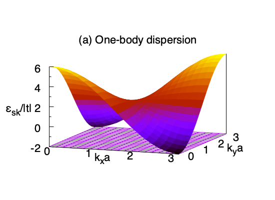
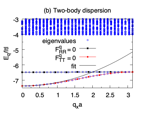
Figure 1: (a) One-body dispersion $\varepsilon_{s\mathbf{k}}$ is shown for the Mielke checkerboard lattice when the lower band is flat. The bands touch at the four corners of the 1st Brillouin zone. (b) Two-body dispersion $E_{\mathbf{q}}$ is shown for $U=5|t|$ as a function of $q_{x}a$ when $q_{y}a=0$. The conditions $F_{RR}^{\mathbf{q}}=0$ and $F_{TT}^{\mathbf{q}}=0$ are in perfect agreement with the upper and lower branches, respectively. The quadratic expansion $E_{\mathbf{q}}=E_{b}+q^{2}/(2m_{b})$ is an excellent fit for the lower branch in the small-$q$ limit.

For the two-body problem of interest in this paper, first we find all possible $E_{\mathbf{q}}$ values by solving the eigenvalue problem that is governed by Eq. (II). The exact solutions are shown in Fig. 1(b) for $U=5|t|$ when $q_{y}a=0$. Note that all of the high-energy bound states have an instability towards a one-body decay in the $-4|t|\leq E_{\mathbf{q}}\leq 12|t|$ region. For this reason we focus only on the low-energy states with $E_{\mathbf{q}}<-4|t|$. In Fig. 1(b) there are two distinct bound-state branches appearing in the two-body problem. In contrast to the upper branch that appears nearly featureless in the shown scale, the lower one disperses quadratically with momentum in the small-$q$ limit. Given that our quadratic expansion $E_{\mathbf{q}}=E_{b}+q^{2}/(2m_{b})$ is an excellent fit around $q=0$, next we analyze both the offset $E_{b}<-4|t|$ of the lower branch and its effective mass $m_{b}>0$ in greater detail.

For this purpose, first we note in Fig. 1(b) that the conditions $F_{RR}^{\mathbf{q}}=0$ and $F_{TT}^{\mathbf{q}}=0$ are in perfect agreement with the upper and lower branches, respectively. This is because the coupling term $F_{TR}^{\mathbf{q}}$ integrates to $0$ when $q_{x}=0$ and/or $q_{y}=0$. Then, in contrast to Eq. (II), we note that Eqs. (22) and (23) offer an analytically tractable approach. For instance one can determine both $E_{b}$ and $m_{b}$ of the lower branch by substituting $E_{\mathbf{q}}=E_{b}+\sum_{ij}q_{i}(\mathbf{m_{b}^{-1}})_{ij}q_{j}/2$ in Eq. (22), and expanding the condition $F_{TT}^{\mathbf{q}}=0$ up to second order in $\mathbf{q}$. Here $(\mathbf{m_{b}^{-1}})_{ij}$ corresponds to the $ij$th element of the inverse of the effective-mass tensor $\mathbf{m_{b}}$ of the lower branch. Thus the condition $F_{TT}^{\mathbf{0}}=0$ for the zeroth-order term leads to a closed-form expression

$$1=\frac{U}{N}\sum_{s\mathbf{k}}\frac{1}{2\varepsilon_{s\mathbf{k}}-E_{b}}$$ (25)

for the $E_{b}$ of the lower branch. Note that the familiar one-band result is recovered by Eq. (25), after setting $d_{\mathbf{k}}=0$ in the one-body dispersion shown in Eq. (16). Similarly the condition $F_{RR}^{\mathbf{0}}=0$ gives an expression for the $E_{b}$ of the upper branch. In Fig. 2(a) we show $E_{b}$ for both the upper and lower branches as a function of $U$. For the lower branch of main interest here, we find that $E_{b}=-4|t|-U/2$ is an excellent fit in the small-$U$ limit but it approaches to $E_{b}=-4|t|-U$ in the large-$U$ limit.

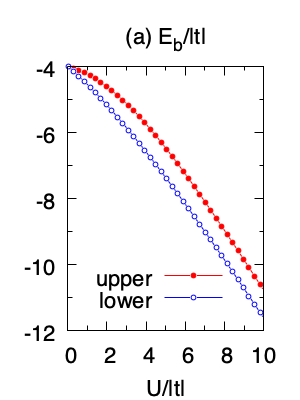
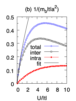
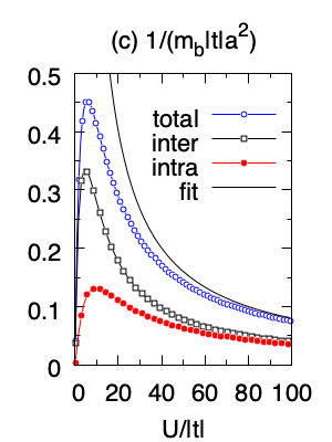
Figure 2: (a) Lowest energy $E_{b}=E_{\mathbf{q}=\mathbf{0}}$ of the bound state is shown for the upper and lower branches as a function of $U$. (b) Inverse of the effective mass $m_{b}$ of the bound state is shown for the lower branch as a function of $U$ together with its intraband and interband contributions, where $1/m_{b}=1/m_{b}^{\mathrm{intra}}+1/m_{b}^{\mathrm{inter}}$. (c) Same as in (b) but with a larger region. Here $m_{b}=5\pi/[Ua^{2}\ln(64|t|/U)]$ and $m_{b}=U/(8a^{2}t^{2})$ fits very well in the small- and large-$U$ limits, respectively.

While the condition $\partial F_{TT}^{\mathbf{q}}/\partial q_{i}|_{\mathbf{q}=\mathbf{0}}=0$ for the first-order term is always satisfied, the condition $\partial^{2}F_{TT}^{\mathbf{q}}/(\partial q_{i}\partial q_{j})|_{\mathbf{q}=\mathbf{0}}=0$ for the second-order term leads to a closed-form expression $(\mathbf{m_{b}^{-1}})_{ij}=(\mathbf{m_{b}^{-1}})_{ij}^{\mathrm{intra}}+(\mathbf{m_{b}^{-1}})_{ij}^{\mathrm{inter}}$ for the effective-mass tensor, where

$$(\mathbf{m_{b}^{-1}})_{ij}^{\mathrm{intra}} =\frac{1}{2}\frac{\sum_{s\mathbf{k}}\frac{\partial^{2}\varepsilon_{s\mathbf{k}}/(\partial k_{i}\partial k_{j})}{(2\varepsilon_{s\mathbf{k}}-E_{b})^{2}}}{\sum_{s\mathbf{k}}\frac{1}{(2\varepsilon_{s\mathbf{k}}-E_{b})^{2}}},$$ (26)

$$(\mathbf{m_{b}^{-1}})_{ij}^{\mathrm{inter}} =-2\frac{\sum_{s\mathbf{k}}\frac{sd_{\mathbf{k}}g_{\mathbf{k}}^{ij}}{(2d_{\mathbf{k}}^{0}-E_{b})(2\varepsilon_{s\mathbf{k}}-E_{b})}}{\sum_{s\mathbf{k}}\frac{1}{(2\varepsilon_{s\mathbf{k}}-E_{b})^{2}}},$$ (27)

are the so-called intraband and interband contributions, respectively. Here $2g_{\mathbf{k}}^{ij}=\partial(\mathbf{d}_{\mathbf{k}}/d_{\mathbf{k}})\partial k_{i}\cdot\partial(\mathbf{d}_{\mathbf{k}}/d_{\mathbf{k}})\partial k_{j}$ is precisely the quantum-metric tensor of the Bloch states torma17a ; iskin19b ; iskin20 . It is truly delightful to note that the expressions Eqs. (26) and (27) are formally equivalent to the ones reported in the recent literature in an entirely different but a related context, i.e., the effective-mass tensor of the Cooper pairs in the presence of helicity bands that is induced by spin-orbit coupling iskin18a . In particular they suggest that while the intraband processes depend only on the one-body band structure, the interband ones are controlled by the quantum geometry of the Bloch states. In addition the familiar one-band result is recovered merely by Eq. (26), after setting $d_{\mathbf{k}}=0$ in the one-body dispersion shown in Eq. (16). This leads not only to $(\mathbf{m_{b}^{-1}})_{ij}^{\mathrm{inter}}=0$ but also to $(\mathbf{m_{b}^{-1}})_{ij}^{\mathrm{intra}}=\delta_{ij}/(2m)$ for the one-body dispersion that is quadratic in $k$, e.g., $d_{\mathbf{k}}^{0}=\varepsilon_{0}+k^{2}/(2m)$, where $\delta_{ij}$ is the Kronecker-delta.

For the specific case of a Mielke checkerboard lattice, $\mathbf{m_{b}}$ turns out to be a diagonal matrix with isotropic elements, leading to $1/m_{b}=1/m_{b}^{\mathrm{intra}}+1/m_{b}^{\mathrm{inter}},$ and they are shown in Fig. 2(b) as a function of $U$. By the trial and error approach, we find that $m_{b}=5\pi/[Ua^{2}\ln(64|t|/U)]$ fits very well in the small-$U$ limit. Since the effective intraband mass of the one-body dispersion diverges for the flat band to begin with, we note that $U\neq 0$ is responsible for $m_{b}\neq\infty$ through the interband processes with the dispersive band, e.g., it can be shown that $(\mathbf{m_{b}^{-1}})_{ij}^{\mathrm{inter}}\approx\frac{U}{N}\sum_{\mathbf{k}}g_{\mathbf{k}}^{ij}[1-U/(4\varepsilon_{+,\mathbf{k}}-2E_{b})]$ in the $U\to 0^{+}$ limit. Here $\frac{1}{N_{c}}\sum_{\mathbf{k}}g_{\mathbf{k}}^{ij}$ diverges by itself due to the touching points, and the second term is crucial for producing a finite effective mass in the Mielke flat band, i.e., it cancels precisely those diverging points. Thus our calculation reveals the quantum-geometric mechanism that gives rise to a finite $m_{b}$ in the $U\to 0^{+}$ limit as long as $U$ is nonzero. However, away from the small-$U$ limit, Fig. 2(b) shows that the intraband processes within the dispersive band also give a similar contribution. The physical mechanism is known to be very different in the large-$U$ limit ohashi08 ; wouters06 ; valiente08 , where the tunneling of the bound state is possible only through virtual dissociation of the pair, and this leads to $m_{b}\sim U/(8a^{2}t^{2})$ as shown in Fig. 2(c).

In particular to the small-$U$ limit, we would like to emphasize that our generic result $m_{b}\propto\mathcal{A}/[U\ln(\mathcal{B}/U)]$ for the non-isolated flat bands is in distinct contrast with that $m_{b}\propto\mathcal{A}/U$ of the isolated ones torma18 , where $\mathcal{A}$ and $\mathcal{B}$ are real constants depending on the lattice structure. To be more precise, it was found that the quadratic expansion of $E_{\mathbf{q}}$ works very well for some isolated flat bands with an offset $E_{b}=-U/N_{b}$ defined from the flat band and an effective-mass tensor $(\mathbf{m_{b}^{-1}})_{ij}=\frac{U}{N}\sum_{\mathbf{k}}g_{\mathbf{k}}^{ij}$ in the small-$U$ limit torma18 . Here $g_{\mathbf{k}}^{ij}$ is the corresponding quantum-metric tensor of the Bloch states in the flat band in the presence of other flat and/or dispersive bands. In comparison to the intraband contribution of Eq. (26) for a non-isolated flat band, there is no such contribution for an isolated flat band in the small-$U$ limit due to the presence of a band gap between the flat band and others. However, we again note that $U\neq 0$ is fully responsible for $m_{b}\neq\infty$ through merely the interband processes with the rest of the Bloch states in the system.

V Conclusion

In summary, above we constructed a variational approach to study the two-body bound-state problem in a generic multi-band lattice, and gave a detailed account of bipartite lattices with an onsite interaction that manifest time-reversal symmetry. For this case we showed that the lowest-energy bound states disperse quadratically with momentum, whose effective-mass tensor has two physically distinct contributions coming from (i) the intraband processes that depend only on the one-body dispersion and (ii) the interband processes that also depend on the quantum-metric tensor of the underlying Bloch states. In particular we applied our theory to the Mielke checkerboard lattice for its simplicity, and revealed how the interband processes help produce a finite effective mass for the bound states in a non-isolated flat band. As an outlook, our theory can be extended to the non-isolated flat bands of Kagome and Lieb lattices that have recently been realized in a number of physical systems jo12 ; nakata12 ; li18 ; diebel16 ; kajiwara16 ; ozawa17 .

References

(1)
L. Balents, C. R. Dean, D. K. Efetov, and A. F. Young,
Superconductivity and strong correlations in moir flat bands,
Nat. Phys. 16, 725 (2020).
(2)
Z. Liu, F. Liu, and Yong-Shi Wu,
Exotic electronic states in the world of flat bands: from theory to material,
Chin. Phys. B 23, 077308 (2014).
(3)
D. Leykam, A. Andreanov, and S. Flach,
Artificial flat band systems: from lattice models to experiments,
Adv. Phys.: X 3, 1473052 (2018).
(4)
H. Tasaki,
From Nagaoka’s Ferromagnetism to Flat-Band Ferromagnetism and Beyond:
An Introduction to Ferromagnetism in the Hubbard Model,
Prog. of Theoretical Physics 99, 489 (1998).
(5)
S. A. Parameswaran, R. Roy, and S. L. Sondhi,
Fractional Quantum Hall Physics in Topological Flat Bands,
Comptes Rendus Physique 14, 816 (2013).
(6)
G.-B. Jo, J. Guzman, C. K. Thomas, P. Hosur, A. Vishwanath, and D. M. Stamper-Kurn,
Ultracold Atoms in a Tunable Optical Kagome Lattice,
Phys. Rev. Lett. 108, 045305 (2012).
(7)
Y. Nakata, T. Okada, T. Nakanishi, and M. Kitano,
Observation of flat band for terahertz spoof plasmons in a metallic Kagomé lattice,
Phys. Rev. B 85, 205128 (2012).
(8)
Z. Li, J. Zhuang, L. Wang, H. Feng, Q. Gao, X. Xu, W. Hao, X. Wang, C. Zhang,
K. Wu, S. X. Dou, L. Chen, Z. Hu, and Y. Du,
Realization of flat band with possible nontrivial topology in electronic Kagome lattice,
Science Advances 4, eaau4511 (2018).
(9)
F. Diebel, D. Leykam, S. Kroesen, C. Denz, and A. S. Desyatnikov
Conical Diffraction and Composite Lieb Bosons in Photonic Lattices,
Phys. Rev. Lett. 116, 183902 (2016).
(10)
S. Kajiwara, Y. Urade, Y. Nakata, T. Nakanishi, and M. Kitano,
Observation of a nonradiative flat band for spoof surface plasmons in a metallic Lieb lattice,
Phys. Rev. B 93, 075126 (2016).
(11)
H. Ozawa, S. Taie, T. Ichinose, and Y. Takahashi,
Interaction-Driven Shift and Distortion of a Flat Band in an Optical Lieb Lattice,
Phys. Rev. Lett. 118, 175301 (2017).
(12)
S. Peotta and P. Törmä,
Superfluidity in topologically nontrivial flat bands,
Nat. Commun. 6, 8944 (2015).
(13)
P. Törmä, L. Liang, and S. Peotta,
Quantum metric and effective mass of a two-body bound state in a flat band,
Phys. Rev. B 98, 220511(R) (2018).
(14)
J. P. Provost and G. Vallee,
Riemannian structure on manifolds of quantum states,
Commun. Math. Phys. 76, 289 (1980).
(15)
M. V. Berry,
The quantum phase, five years after in Geometric Phases in Physics,
edited by A. Shapere and F. Wilczek (World Scientific, Singapore, 1989).
(16)
R. Resta,
The insulating state of matter: A geometrical theory,
Eur. Phys. J. B 79, 121 (2011).
(17)
M. Iskin,
Quantum metric contribution to the pair mass in spin-orbit coupled Fermi superfluids,
Phys. Rev. A 97, 033625 (2018).
(18)
Z. Wang, G. Chaudhary, Q. Chen, and K. Levin,
Quantum geometric contributions to the BKT transition: Beyond mean field theory,
Phys. Rev. B 102, 184504 (2020).
(19)
M. Iskin,
Origin of flat-band superfluidity on the Mielke checkerboard lattice,
Phys. Rev. A 99, 053608 (2019).
(20)
Y. Ohashi,
Tunneling properties of a bound pair of Fermi atoms in an optical lattice,
Phys. Rev. A 78, 063617 (2008).
(21)
M. Iskin,
Collective excitations of a BCS superfluid in the presence of two sublattices,
Phys. Rev. A 101, 053631 (2020).
(22)
L. Liang, T. I. Vanhala, S. Peotta, T. Siro, A. Harju, and P. Törmä,
Band geometry, Berry curvature, and superfluid weight,
Phys. Rev. B 95, 024515 (2017).
(23)
M. Wouters and G. Orso,
Two-body problem in periodic potentials,
Phys. Rev. A 73, 012707 (2006).
(24)
M. Valiente and D. Petrosyan,
Two-particle states in the Hubbard model,
J. Phys. B: At. Mol. Opt. Phys. 41, 161002 (2008).