High Order Numerical Homogenization for Dissipative Ordinary Differential Equations

Abstract

We propose a high order numerical homogenization method for dissipative ordinary differential equations (ODEs) containing two time scales. Essentially, only first order homogenized model globally in time can be derived. To achieve a high order method, we have to adopt a numerical approach in the framework of the heterogeneous multiscale method (HMM). By a successively refined microscopic solver, the accuracy improvement up to arbitrary order is attained providing input data smooth enough. Based on the formulation of the high order microscopic solver we derived, an iterative formula to calculate the microscopic solver is then proposed. Using the iterative formula, we develop an implementation to the method in an efficient way for practical applications. Several numerical examples are presented to validate the new models and numerical methods.

34E13, 65L04

1 Introduction

Multiple-time-scale problems are often encountered in many disciplines such as chemical kinetics [23], molecular dynamics [4, 32] and celestial mechanics [21]. There are many studies concerning stiff systems of ordinary differential equations (ODEs), especially those with two time scales. In general, these systems can be divided into two categories [9]. One is dissipative systems where fast variables tend to the stationary state at an exponential rate. The other one is oscillatory systems where fast variables oscillate in some orbits.

It is impossible to resolve all the time scales and capture all the variables numerically due to limited computing power. In many problems, we are only interested in the dynamics of slow macroscopic variables. There is some work on designing efficient numerical algorithms for stiff ODEs, such as implicit Runge-Kutta methods [30], backward differentiation formulas [2], Rosenbrock methods [20] and projective methods [14].

It is well known [24] that, as $\varepsilon\rightarrow 0$, the dynamics of slow variables satisfy a limiting equation, which can be obtained by averaging methods. For simple systems, the limiting equation can be derived by analytical tools. For complex systems, however, we have to sample the fast variables to approximate the limiting equation. A famous method of this type is the heterogeneous multiscale method [10, 1, 11]. In HMM, there is a microscopic solver to sample the fast variables, and a macroscopic solver to evolve the slow variables. Some results of numerical analysis on this method can be found in [9]. There are three main sources of errors of HMM, including modeling error, sampling error and truncation error of the macroscopic solver. The modeling error is of order $\mathcal{O}(\varepsilon)$. When $\varepsilon$ is sufficiently small, the modeling error is small enough. However, when $\varepsilon$ is relatively but not extremely small, the modeling error is not ignorable. Therefore, it is necessary to propose a correction model to reduce the modeling error in this situation.

There have been several attempts to reduce modeling error in multiscale method. For example, in [6], they use B-series to derive a high-order stroboscopic averaged equations for a kind of highly oscillatory systems. In [19, 31], they develop a first order correction model for sediment transport in sub-critical case, where the modeling error can be reduced to $\mathcal{O}(\varepsilon^{2})$.

In this paper, we develop a novel high-order correction model and the corresponding numerical algorithms for stiff dissipative system of ODEs. Our studies begin with the theory of invariant manifold for ODEs [15, 25]. It can be proved that the invariant manifold is a global attractor. Actually, the microscopic solver of HMM is designed to find an approximation to the invariant manifold with an error of $\mathcal{O}(\varepsilon)$. In order to derive the correction models, we need to find high-order approximations to the invariant manifold. By the asymptotic approximation method, the analytical expressions of the first several terms in the formal expansion can be obtained. We can prove that this approximation shares similar properties to the invariant manifold. In other words, the trajectories tend to this approximation to invariant manifold at an exponential rate. Once the trajectories are close to this approximation, then they can be approximated by a reduced model over a finite time horizon. However, the terms obtained by the formal expansion are too complicated to be implemented, especially for higher-order methods. In addition, it requires the evaluation of high-order derivatives. We design an iterative formula for the sake of practicality. We can prove that the iterative method matches with the formal expansion in some sense. We can also prove that the approximation accuracy reaches $\mathcal{O}(\varepsilon^{k+1})$ after $k$ iteration steps. By the technology of numerical derivatives, we design a recursion method using the iterative scheme. We also present some numerical analysis on our algorithms.

The rest of this paper is arranged as follows. In Section 2, we briefly introduce the multiscale dissipative systems and the heterogeneous multiscale methods. In Section 3, we present our models for high-order homogenization and analyze their properties. In Section 4, we develop two types of algorithms in the framework of HMM. Some numerical analysis is presented in Section 5. Numerical results are shown in Section 6 and the paper ends with a brief summary and conclusion in Section 7.

2 Preliminaries

2.1 Dissipative systems

Let us consider the following ODEs with scale separation [25]:

(1) $$\left\{\begin{aligned} &\dfrac{\mathrm{d}x}{\mathrm{d}t}=f(x,y),\\ &\dfrac{\mathrm{d}y}{\mathrm{d}t}=\frac{1}{\varepsilon}g(x,y),\\ &x|_{t=0}=x_{0},\ y|_{t=0}=y_{0},\end{aligned}\right.$$

where $x\in\mathbb{R}^{n_{x}}$ is the slow variable and $y\in\mathbb{R}^{n_{y}}$ is the fast variable, $n_{x}$ and $n_{y}$ are the dimension of $x$ and $y$, respectively. The parameter $0<\varepsilon\leq\varepsilon_{0}\ll 1$ characterizes the separation of time scales. Let $y^{x}$ be the solution of

(2) $$\left\{\begin{aligned} &\dfrac{\mathrm{d}y^{x}}{\mathrm{d}t}=\frac{1}{\varepsilon}g(x,y^{x}),\\ &y^{x}|_{t=0}=y_{0},\end{aligned}\right.$$

for any $x$ fixed. Suppose that ${\mathrm{d}}\mu^{x}(y)$ is the corresponding invariant measure of Eq. 2 satisfying that for any $\phi\in\mathcal{L}^{1}(\mathbb{R}^{n_{y}};{\mathrm{d}}\mu^{x})$,

$$\lim\limits_{T\rightarrow+\infty}\frac{1}{T}\int_{0}^{T}\phi(y^{x}(t))\,{\mathrm{d}}t=\int_{\mathbb{R}^{n_{y}}}\phi(y)\,{\mathrm{d}}\mu^{x}(y),\ \text{ for }\mu^{x}-\text{a.e. }y_{0}\in\mathbb{R}^{n_{y}}.$$

Let

$$F(x)=\lim\limits_{T\rightarrow+\infty}\frac{1}{T}\int_{0}^{T}f(x,y^{x}(t))\,{\mathrm{d}}t=\int_{\mathbb{R}^{n_{y}}}f(x,y)\,{\mathrm{d}}\mu^{x}(y).$$

Under some appropriate assumptions [24], the trajectory of $x(t)$ tends to a solution of the limiting equation

(3) $$\dfrac{\mathrm{d}X_{0}}{\mathrm{d}t}=F(X_{0}),$$

as $\varepsilon\rightarrow 0$ in some sense.

Since now on, we assume the regularity of the functions $f$ and $g$. Precisely, we assume that The functions $f$ and $g$ are sufficiently smooth. In addition, there exists $K\in\mathbb{N}\setminus\{0\}$ such that

$$f\in W^{K,\infty}(\mathbb{R}^{n_{x}}\times\mathbb{R}^{n_{y}},\mathbb{R}^{n_{x}}),\quad\nabla g\in W^{K,\infty}(\mathbb{R}^{n_{x}}\times\mathbb{R}^{n_{y}},\mathbb{R}^{n_{y}\times(n_{x}+n_{y})}).$$

Furthermore, we always have the following assumption for $g$. For each $x\in\mathbb{R}^{n_{x}}$, there exists $\gamma(x)\in\mathbb{R}^{n_{y}}$ such that

(4) $$g(x,\gamma(x))=0.$$

In addition, there exists $\beta>0$ such that

(5) $$\left\langle{g(x,y)-g(x,\tilde{y})},{y-\tilde{y}}\right\rangle\leq-\beta|y-\tilde{y}|^{2},\quad\forall x\in\mathbb{R}^{n_{x}},\forall y,\tilde{y}\in\mathbb{R}^{n_{y}}.$$

By Section 2.1, one can see that the dynamic for $y$ with $x$ fixed has a unique, globally exponentially attracting point [25]. At this time, the system Eq. 1 is called a dissipative system. It is clear that the invariant measure ${\mathrm{d}}\mu^{x}(y)$ at fixed $x$ is a one-point distribution at $y=\gamma(x)$. In addition, one has that $F(x)=f(x,\gamma(x))$. It was pointed out in [25] that, under some appropriate assumptions, the modeling error between the solutions of Eq. 1 and Eq. 3 is of order $\mathcal{O}(\varepsilon)$ in a finite time horizon.

Remark 2.1.

Let $\tilde{g}_{x}=g(x,\cdot):\mathbb{R}^{n_{y}}\rightarrow\mathbb{R}^{n_{y}}$. If $g(x,y)$ satisfies Eq. 5, then we say that $\tilde{g}_{x}$ is a $\beta$-strongly dissipative operator or $-\tilde{g}_{x}$ is a $\beta$-strongly monotonic operator on $\mathbb{R}^{n_{y}}$ by the definitions in [27, 3]. It can be deduced [17] that, if $\tilde{g}_{x}$ is $L$-Lipschitz continuous, and $\beta$-strongly dissipative, then $\tilde{g}_{x}$ is a bijection on $\mathbb{R}^{n_{y}}$, $\tilde{g}_{x}^{-1}:\mathbb{R}^{n_{y}}\rightarrow\mathbb{R}^{n_{y}}$ is $\frac{1}{\beta}$-Lipschitz continuous, and $\frac{\beta}{L^{2}}$-strongly dissipative.

2.2 Heterogeneous multiscale method

The heterogeneous multiscale method (HMM) is a general strategy for multiscale problems [1, 9]. It makes use of two solvers: a macroscopic solver and a microscopic solver. Let us consider the system Eq. 1. As a macroscopic solver, a conventional explicit ODE solver is chosen to evolve Eq. 3. For example, take the forward Euler method with a time step $\Delta t$ as the macroscopic solver, which can be expressed as

$$x_{n+1}=x_{n}+\Delta tF(x_{n}).$$

To evaluate $F(x_{n})$, a microscopic solver is chosen to resolve the microscopic scale. In the case of the forward Euler method with a time step $\delta t$ , one gets that

(6a) $$y_{n,m+1}=y_{n,m}+\frac{\delta t}{\varepsilon}g(x_{n},y_{n,m}),\ m=0,1,\ldots,M-1,$$

(6b) $$y_{n,0}\text{ suitably chosen.}$$

Then one can estimate $F(x_{n})$ by

$$F(x_{n})\approx\sum_{m=0}^{M}K_{m,M}f(x_{n},y_{n,m}),$$

where the weights $\{K_{m,M}\}$ should satisfy the constraint $\sum_{m=0}^{M}K_{m,M}=1.$ As suggested in [9], for dissipative systems, one can choose the weights as

$$K_{m,M}=0,\ m=0,1,\ldots,M-1,$$

$$K_{M,M}=1.$$

In other words, one may estimate that $F(x_{n})=f(x_{n},\gamma(x_{n}))\approx f(x_{n},y_{n,M})$. In this situation, the microscopic solver Eq. 6 can be regarded as a nonlinear solver for the equation $g(x_{n},y)=0$ with respect to $y$.

3 Models

In this section, we present our high-order correction models of the limiting equation Eq. 3 and analyze their properties. We begin with asymptotic approximation to the invariant manifold and then design an iterative formula to generate high-order correction models automatically. The modeling error can be reduced to $\mathcal{O}(\varepsilon^{k+1})$ in the $k$th-order correction model.

3.1 Invariant manifold

To begin with, we introduce the concept of invariant manifold [25]. Assuming that there exists an invariant set $\mathcal{S}_{\varepsilon}$ of Eq. 1, and that it can be represented as a smooth graph over $x$, namely, there exists a function $\Gamma:\mathbb{R}^{n_{x}}\times(0,\varepsilon_{0}]\rightarrow\mathbb{R}^{n_{y}}$ that is differentiable with respect to $x$, such that

$$\mathcal{S}_{\varepsilon}=\left\{(x,y):y=\Gamma(x,\varepsilon),\ x\in\mathbb{R}^{n_{x}}\right\},\quad\forall\varepsilon\in(0,\varepsilon_{0}].$$

This implies that

(7) $$g(x,\Gamma(x,\varepsilon))=\varepsilon\nabla_{x}\Gamma(x,\varepsilon)f(x,\Gamma(x,\varepsilon)),\ \forall x\in\mathbb{R}^{n_{x}}.$$

The equation Eq. 7 plays a central role in our discussions. It can be proved under some appropriate conditions that $\mathcal{S}_{\varepsilon}$ is a global attractor of the system Eq. 1, that is, for any initial values,

(8) $$\lim\limits_{t\rightarrow+\infty}|y(t)-\Gamma(x(t),\varepsilon)|=0.$$

Proposition 3.1.

Suppose that $\nabla_{y}f(x,y)$ and $\nabla_{x}\Gamma(x,\varepsilon)$ are bounded, then $\mathcal{S}_{\varepsilon}$ is a global attractor of the system Eq. 1 for sufficiently small $\varepsilon$.

Proof 3.2.

Assuming that $\big{|}\nabla_{y}f(x,y)\big{|}\leq C$ and $\big{|}\nabla_{x}\Gamma(x,\varepsilon)\big{|}\leq C$. Let $z(t)=y(t)-\Gamma(x(t),\varepsilon)$. By Section 2.1, one gets that

$$\frac{1}{2}\dfrac{\mathrm{d}|z|^{2}}{\mathrm{d}t}=\left\langle{z},{\dfrac{\mathrm{d}z}{\mathrm{d}t}}\right\rangle=\left\langle{y-\Gamma(x,\varepsilon)},{\frac{1}{\varepsilon}g(x,y)-\nabla_{x}\Gamma(x,\varepsilon)f(x,y)}\right\rangle$$

$$= \left\langle{y-\Gamma(x,\varepsilon)},{\frac{1}{\varepsilon}g(x,y)-\frac{1}{\varepsilon}g(x,\Gamma(x,\varepsilon))}\right\rangle$$

$$\qquad\quad+\left\langle{y-\Gamma(x,\varepsilon)},{\nabla_{x}\Gamma(x,\varepsilon)f(x,\Gamma(x,\varepsilon))-\nabla_{x}\Gamma(x,\varepsilon)f(x,y)}\right\rangle$$

$$\leq \left(-\frac{\beta}{\varepsilon}+C^{2}\right)|z|^{2}.$$

This implies that $|z(t)|^{2}\leq e^{-\frac{\beta}{\varepsilon}t}|z(0)|^{2}$ when $0<\varepsilon\leq\min\left\{\frac{\beta}{2C^{2}},\varepsilon_{0}\right\}$, and then the proof is completed.

Proposition 3.1 says that the trajectory of $(x(t),y(t))$ tends to the set $\mathcal{S}_{\varepsilon}$ at an exponential rate. Later we refer to this type of properties as the attractive property. Since $\mathcal{S}_{\varepsilon}$ is invariant, one obtains that, if the initial values lie on $\mathcal{S}_{\varepsilon}$, then the trajectory of $(x(t),y(t))$ stays on $\mathcal{S}_{\varepsilon}$ for any $t>0$. At this time, one may use

(9) $$\dfrac{\mathrm{d}X}{\mathrm{d}t}=f(X,\Gamma(X,\varepsilon))$$

rather than Eq. 1 to calculate the trajectory of $x(t)$. In other words, the system Eq. 1 can be decoupled. We refer to this type of properties as the decouplable property. It should be emphasized that Proposition 3.1 depends on the existence of $\Gamma(x,\varepsilon)$, however, the rest of this article does not depend on it.

As an example, we study the invariant manifold of the linearized equation of the system Eq. 1.

Example 3.3.

We consider the following linear equation as a special case of the system Eq. 1:

(10) $$\left\{\begin{aligned} &\dfrac{\mathrm{d}x}{\mathrm{d}t}=A_{11}x+A_{12}y+b_{1},\\ &\dfrac{\mathrm{d}y}{\mathrm{d}t}=\frac{1}{\varepsilon}(A_{21}x+A_{22}y+b_{2}),\end{aligned}\right.$$

where $A_{11}\in\mathbb{R}^{n_{x}\times n_{x}}$, $A_{12}\in\mathbb{R}^{n_{x}\times n_{y}}$, $A_{21}\in\mathbb{R}^{n_{y}\times n_{x}}$, $A_{22}\in\mathbb{R}^{n_{y}\times n_{y}}$, $b_{1}\in\mathbb{R}^{n_{x}}$, $b_{2}\in\mathbb{R}^{n_{y}}$. We assume that $A_{22}$ is a negative definite matrix to satisfy Section 2.1.

Suppose that the function $\Gamma(x,\varepsilon)$ has a form of $\Gamma(x,\varepsilon)=Cx+d$, where $C=C(\varepsilon)\in\mathbb{R}^{n_{y}\times n_{x}}$ and $d=d(\varepsilon)\in\mathbb{R}^{n_{y}}$. By Eq. 7, one gets the following equations:

(11a) $$\varepsilon CA_{12}C+\varepsilon CA_{11}-A_{22}C-A_{21}=0,$$

(11b) $$(A_{22}-\varepsilon CA_{12})d=\varepsilon Cb_{1}-b_{2}.$$

It is known that Eq. 11a is an algebraic matrix Riccati equation [13, 28]. We can prove the well-posedness of Eq. 11 when $\varepsilon$ is sufficiently small. See Theorem A.1 in Appendix A.

3.2 Asymptotic approximation

In this part, we consider the asymptotic approximation to $\Gamma(x,\varepsilon)$. We calculate the first several terms in the formal asymptotic expansion, and then prove the attractive property and the decouplable property of this approximation.

3.2.1 Formal expansions

Suppose that $\Gamma(x,\varepsilon)$ satisfies Eq. 7. We try formal expansions of the form

(12a) $$\Gamma(x,\varepsilon)=\gamma_{0}(x)+\varepsilon\gamma_{1}(x)+\varepsilon^{2}\gamma_{2}(x)+\mathcal{O}(\varepsilon^{3}),$$

(12b) $$\nabla_{x}\Gamma(x,\varepsilon)=\nabla\gamma_{0}(x)+\varepsilon\nabla\gamma_{1}(x)+\varepsilon^{2}\nabla\gamma_{2}(x)+\mathcal{O}(\varepsilon^{3}).$$

By Section 2.1, we specify that $\gamma_{0}(x)=\gamma(x)$. By Taylor’s expansion of $g(x,y)$ at $(x,\gamma(x))$ and the formal expansion in Eq. 12a, one notices that the left-hand side of Eq. 7 can be written as

(13) $$g(x,\Gamma(x,\varepsilon))$$

$$= g(x,\gamma(x)+\varepsilon\gamma_{1}(x)+\varepsilon^{2}\gamma_{2}(x)+\mathcal{O}(\varepsilon^{3}))$$

$$= \varepsilon G_{y}(x)\gamma_{1}(x)+\varepsilon^{2}\left(G_{y}(x)\gamma_{2}(x)+\frac{1}{2}\left[\sum_{j,k=1}^{n_{y}}G_{yy}^{i,j,k}\gamma_{1}^{j}(x)\gamma_{1}^{k}(x)\right]_{i=1}^{n_{y}}\right)+\mathcal{O}(\varepsilon^{3}),$$

where $G_{y}(x)=[G_{y}^{i,j}(x)]_{i,j=1}^{n_{y}}=\left[\frac{\partial g^{i}}{\partial y^{j}}(x,\gamma(x))\right]_{i,j=1}^{n_{y}}$ and $G_{yy}(x)=[G_{yy}^{i,j,k}(x)]_{i,j,k=1}^{n_{y}}=\left[\frac{\partial^{2}g^{i}}{\partial y^{j}\partial y^{k}}(x,\gamma(x))\right]_{i,j,k=1}^{n_{y}}$. Similarly, by Taylor’s expansion of $f(x,y)$ at $(x,\gamma(x))$ and the formal expansions in Eq. 12, one obtains that the right-hand side of Eq. 7 can be written as

(14) $$\varepsilon\nabla_{x}\Gamma(x,\varepsilon)f(x,\Gamma(x,\varepsilon))$$

$$= \varepsilon\left(\nabla\gamma(x)+\varepsilon\nabla\gamma_{1}(x)\right)\left(F(x)+\varepsilon F_{y}(x)\gamma_{1}(x)\right)+\mathcal{O}(\varepsilon^{3})$$

$$= \varepsilon\nabla\gamma(x)F(x)+\varepsilon^{2}\left(\nabla\gamma(x)F_{y}(x)\gamma_{1}(x)+\nabla\gamma_{1}(x)F(x)\right)+\mathcal{O}(\varepsilon^{3}),$$

where $F_{y}(x)=[F_{y}^{i,j}(x)]_{i=1,j=1}^{n_{x},n_{y}}=\left[\frac{\partial f^{i}}{\partial y^{j}}(x,\gamma(x))\right]_{i=1,j=1}^{n_{x},n_{y}}$. By Section 2.1, $G_{y}(x)$ is invertible. By comparing Eq. 13 and Eq. 14, one gets the analytic expressions of $\gamma_{0}(x)$, $\gamma_{1}(x)$ and $\gamma_{2}(x)$:

(15a) $$\gamma_{0}(x)=\gamma(x),$$

(15b) $$\gamma_{1}(x)=G_{y}(x)^{-1}\nabla\gamma(x)F(x),$$

(15c) $$\gamma_{2}(x)=G_{y}(x)^{-1}\Bigg{(}\nabla\gamma(x)F_{y}(x)\gamma_{1}(x)$$

$$\qquad\qquad\qquad+\nabla\gamma_{1}(x)F(x)-\frac{1}{2}\Bigg{[}\sum_{j,k=1}^{n_{y}}G_{yy}^{i,j,k}\gamma_{1}^{j}(x)\gamma_{1}^{k}(x)\Bigg{]}_{i=1}^{n_{y}}\Bigg{)}.$$

Remark 3.4.

By taking gradient of both sides of Eq. 4, one obtains that

(16) $$G_{x}(x)+G_{y}(x)\nabla\gamma(x)=0,$$

where $G_{x}(x)=[G_{x}^{i,j}(x)]_{i=1,j=1}^{n_{y},n_{x}}=\left[\frac{\partial g^{i}}{\partial x^{j}}(x,\gamma(x))\right]_{i=1,j=1}^{n_{y},n_{x}}$. Therefore, one can obtain that

$$\nabla\gamma(x)=-G_{y}(x)^{-1}G_{x}(x).$$

This implies that $\gamma_{1}(x)$, $\nabla\gamma_{1}(x)$ and $\gamma_{2}(x)$ can be rewritten as algebraic expressions of function values and derivatives of $f(x,y)$ and $g(x,y)$ at $(x,\gamma(x))$. Therefore, one can obtain that $\gamma$, $\gamma_{1}$ and $\gamma_{2}$ are sufficiently smooth. In addition, by Sections 2.1 and 2.1, and the expressions in Eq. 15, one can deduce that $\nabla\gamma\in W^{K,\infty}$, $\gamma_{1}\in W^{K,\infty}$ and $\gamma_{2}\in W^{K-1,\infty}$. (See Lemmas in Section C.1).

3.2.2 Properties

As an approximation to $\Gamma(x,\varepsilon)$, the function $\tilde{\Gamma}_{2}(x,\varepsilon):=\gamma(x)+\varepsilon\gamma_{1}(x)+\varepsilon^{2}\gamma_{2}(x)$ should share similar properties with $\Gamma(x,\varepsilon)$. Now we make the above statement rigorous. In this part, we let $\mathcal{S}_{\varepsilon}^{(2)}:=\{(x,y):y=\tilde{\Gamma}_{2}(x,\varepsilon),\ x\in\mathbb{R}^{n_{x}}\}$ and $z(t)=y(t)-\tilde{\Gamma}_{2}(x(t),\varepsilon)$.

The attractive property that is parallel to Proposition 3.1 can be formulated as in Theorem 3.5, which says that the system goes quickly from arbitrary initial values into a small vicinity of the approximate invariant manifold $\mathcal{S}_{\varepsilon}^{(2)}$.

Theorem 3.5.

There exists a constant $C>0$ independent of $\varepsilon$ such that

$$|z(t)|^{2}\leq C\varepsilon^{6}+e^{-\frac{\beta}{\varepsilon}t}|z(0)|^{2},$$

for sufficiently small $\varepsilon$. In particular, as long as $t$ is sufficiently large, then $|z(t)|=\mathcal{O}(\varepsilon^{3})$.

Proof 3.6.

By Taylor’s expansion of $f(x,y)$ and $g(x,y)$ at $(x,\gamma(x))$, one gets that

(17) $$\frac{1}{\varepsilon}g(x,\tilde{\Gamma}_{2}(x,\varepsilon))-\nabla_{x}\tilde{\Gamma}_{2}(x,\varepsilon)f(x,\tilde{\Gamma}_{2}(x,\varepsilon))$$

$$= G_{y}(x)\left(\gamma_{1}(x)+\varepsilon\gamma_{2}(x)\right)+\frac{1}{2}\varepsilon\left[\sum_{j,k=1}^{n_{y}}G_{yy}^{i,j,k}\gamma_{1}^{j}(x)\gamma_{1}^{k}(x)\right]_{i=1}^{n_{y}}$$

$$\quad\quad-\left(\nabla\gamma(x)+\varepsilon\nabla\gamma_{1}(x)\right)\left(F(x)+\varepsilon F_{y}(x)\gamma_{1}(x)\right)+\mathcal{O}(\varepsilon^{2})$$

$$= \left(G_{y}(x)\gamma_{1}(x)-\nabla\gamma(x)F(x)\right)$$

$$\quad\quad+\varepsilon\Bigg{(}G_{y}(x)\gamma_{2}(x)+\frac{1}{2}\Bigg{[}\sum_{j,k=1}^{n_{y}}G_{yy}^{i,j,k}\gamma_{1}^{j}(x)\gamma_{1}^{k}(x)\Bigg{]}_{i=1}^{n_{y}}$$

$$\qquad\qquad\qquad\qquad\qquad-\nabla\gamma(x)F_{y}(x)\gamma_{1}(x)-\nabla\gamma_{1}(x)F(x)\Bigg{)}+\mathcal{O}(\varepsilon^{2})$$

$$= \mathcal{O}(\varepsilon^{2}),$$

where $\mathcal{O}(\varepsilon^{2})$ can be controlled uniformly thanks to Section 2.1. By Section 2.1, Remark 3.4 and Eq. 17, there exists a constant $C_{1}>0$ such that

$$\frac{1}{2}\dfrac{\mathrm{d}|z|^{2}}{\mathrm{d}t}=\left\langle{z},{\dfrac{\mathrm{d}z}{\mathrm{d}t}}\right\rangle=\left\langle{y-\tilde{\Gamma}_{2}(x,\varepsilon)},{\frac{1}{\varepsilon}g(x,y)-\nabla_{x}\tilde{\Gamma}_{2}(x,\varepsilon)f(x,y)}\right\rangle$$

$$= \left\langle{y-\tilde{\Gamma}_{2}(x,\varepsilon)},{\frac{1}{\varepsilon}g(x,y)-\frac{1}{\varepsilon}g(x,\tilde{\Gamma}_{2}(x,\varepsilon))}\right\rangle$$

$$\quad\quad+\left\langle{y-\tilde{\Gamma}_{2}(x,\varepsilon)},{\frac{1}{\varepsilon}g(x,\tilde{\Gamma}_{2}(x,\varepsilon))-\nabla_{x}\tilde{\Gamma}_{2}(x,\varepsilon)f(x,\tilde{\Gamma}_{2}(x,\varepsilon))}\right\rangle$$

$$\quad\quad+\left\langle{y-\tilde{\Gamma}_{2}(x,\varepsilon)},{\nabla_{x}\tilde{\Gamma}_{2}(x,\varepsilon)(f(x,\tilde{\Gamma}_{2}(x,\varepsilon))-f(x,y))}\right\rangle$$

$$\leq \left(-\frac{\beta}{\varepsilon}+C_{1}\right)|z|^{2}+C_{1}\varepsilon^{2}|z|\leq-\frac{\beta}{2\varepsilon}|z|^{2}+\frac{C_{1}^{2}}{\beta}\varepsilon^{5},$$

where $0<\varepsilon\leq\min\left\{\frac{\beta}{4C_{1}},\varepsilon_{0}\right\}$. Here the last inequality is due to the Cauchy–Schwarz inequality. By Gronwall’s inequality, one gets that

$$|z(t)|^{2}\leq\frac{2C_{1}^{2}}{\beta^{2}}\varepsilon^{6}(1-e^{-\frac{\beta}{\varepsilon}t})+e^{-\frac{\beta}{\varepsilon}t}|z(0)|^{2},$$

which completes the proof.

Now we consider the decouplable property. Substituting $\tilde{\Gamma}_{2}(x,\varepsilon)$ for $\Gamma(x,\varepsilon)$ in Eq. 9, one obtains the following equation:

(18) $$\dfrac{\mathrm{d}X_{2}}{\mathrm{d}t}=f(X_{2},\tilde{\Gamma}_{2}(X_{2},\varepsilon)).$$

One may surmise that, if the initial values are sufficiently close to $\mathcal{S}_{\varepsilon}^{(2)}$, then one may use Eq. 18 to approximate the trajectory of $x(t)$ in some sense. To be rigorous, we have Theorem 3.7.

Theorem 3.7.

There exists a constant $C>0$ independent of $\varepsilon$ such that

$$|x(t)-X_{2}(t)|^{2}\leq e^{Ct}\left(|x(0)-X_{2}(0)|^{2}+\varepsilon^{6}+\frac{\varepsilon}{\beta}|z(0)|^{2}\right),$$

for sufficiently small $\varepsilon$. In particular, if $|x(0)-X_{2}(0)|=\mathcal{O}(\varepsilon^{3})$ and $|z(0)|=\mathcal{O}(\varepsilon^{\frac{5}{2}})$, then $|x(t)-X_{2}(t)|=\mathcal{O}(\varepsilon^{3})$ for $t\sim\mathcal{O}(1)$.

Proof 3.8.

Since $\nabla_{x}f(x,y)$, $\nabla_{y}f(x,y)$ and $\nabla_{x}\tilde{\Gamma}_{2}(x,\varepsilon)$ are all bounded, then there exists a constant $C_{1}>0$ such that

$$\left|\dfrac{\mathrm{d}(x-X_{2})}{\mathrm{d}t}\right|=|f(x,y)-f(X_{2},\tilde{\Gamma}_{2}(X_{2},\varepsilon))|$$

$$\leq |f(x,z+\tilde{\Gamma}_{2}(x,\varepsilon))-f(x,\tilde{\Gamma}_{2}(X_{2},\varepsilon))|+|f(x,\tilde{\Gamma}_{2}(X_{2},\varepsilon))-f(X_{2},\tilde{\Gamma}_{2}(X_{2},\varepsilon))|$$

$$\leq C_{1}|z|+C_{1}|x-X_{2}|.$$

Then one obtains that

$$\frac{1}{2}\dfrac{\mathrm{d}|x-X_{2}|^{2}}{\mathrm{d}t}=\left\langle{x-X_{2}},{\dfrac{\mathrm{d}(x-X_{2})}{\mathrm{d}t}}\right\rangle$$

$$\leq |x-X_{2}|\cdot\left|\dfrac{\mathrm{d}(x-X_{2})}{\mathrm{d}t}\right|\leq C_{1}|z|\cdot|x-X_{2}|+C_{1}|x-X_{2}|^{2}.$$

Therefore, by Theorem 3.5 and Cauchy-Schwarz inequality, there exists a constant $C>0$ such that

$$\dfrac{\mathrm{d}|x-X_{2}|^{2}}{\mathrm{d}t}\leq C(|x-X_{2}|^{2}+\varepsilon^{6})+e^{-\frac{\beta}{\varepsilon}t}|z(0)|^{2}.$$

By Gronwall’s inequality,

$$|x(t)-X_{2}(t)|^{2}\leq e^{Ct}|x(0)-X_{2}(0)|^{2}+\varepsilon^{6}(e^{Ct}-1)+\frac{e^{Ct}-e^{-\frac{\beta}{\varepsilon}t}}{\frac{\beta}{\varepsilon}+C}|z(0)|^{2},$$

which completes the proof.

Remark 3.9.

Now we look back on what Theorems 3.5 and 3.7 tell us. Theorem 3.5 says that, no matter what the initial values are, the trajectory of $(x(t),y(t))$ always tends to a state where $|y-\tilde{\Gamma}_{2}(x,\varepsilon)|=\mathcal{O}(\varepsilon^{3})$ at an exponential rate. Theorem 3.7 says that, once the trajectory arrives at this state, one may use Eq. 18, which is not stiff, to approximate the trajectory of $x(t)$ in a finite time horizon with an accuracy of $\mathcal{O}(\varepsilon^{3})$. In the literature, this phenomenon is referred as an initial layer or a boundary layer [25, 26, 29, 8, 22]. This remark plays a guiding role in designing our numerical algorithms later.

Remark 3.10.

The properties of $\tilde{\Gamma}_{2}(x,\varepsilon)$ are studied in this part. One may guess that $\tilde{\Gamma}_{k}(x,\varepsilon):=\sum_{j=0}^{k}\varepsilon^{j}\gamma_{j}(x)$ should have similar properties. However, it is expected that the expression of $\gamma_{k}(x)$ is very complex when $k$ is large. In addition, the evaluation of high-order derivatives is involved in the expressions of $\gamma_{k}(x)$. It is not convenient to conduct theoretical analysis or to design numerical algorithms at this time.

3.3 An iterative method

In this part, an iterative method is presented to approximate the invariant manifold $\mathcal{S}_{\varepsilon}$. We put forward an iterative formula, which can be used to produce a series of successively refined approximations to $\Gamma(x,\varepsilon)$. This method overcomes the difficulties in Remark 3.10 due to its concise form. It can be proved theoretically that this method is consistent with asymptotic approximation in some sense, and that the approximation accuracy reaches $\mathcal{O}(\varepsilon^{k+1})$ after $k$ iteration steps.

3.3.1 An iterative formula

Inspired by Eq. 7, we propose the following fixed-point iterative formula to approximate $\Gamma(x,\varepsilon)$:

(19a) $$\Gamma_{0}(x,\varepsilon)=\gamma(x),$$

(19b) $$g(x,\Gamma_{k+1}(x,\varepsilon))=\varepsilon\nabla_{x}\Gamma_{k}(x,\varepsilon)f(x,\Gamma_{k}(x,\varepsilon)),\ k=0,1,2,\ldots.$$

Remark 2.1 implies the existence and uniqueness of the solution $\Gamma_{k+1}(x,\varepsilon)$ of Eq. 19b, since $g(x,\cdot)$ is Lipschitz continuous and strongly dissipative. Using the notations in Remark 2.1, one can write Eq. 19b as

$$\Gamma_{k+1}(x,\varepsilon)=\tilde{g}_{x}^{-1}\left(\varepsilon\nabla_{x}\Gamma_{k}(x,\varepsilon)f(x,\Gamma_{k}(x,\varepsilon))\right).$$

3.3.2 Relationships with asymptotic approximation

In this part, we study the relationships between the iterative formula Eq. 19 and asymptotic approximation. It can be proved that the iterative formula can produce approximations in Eq. 15 in the first two iteration steps. The proof of Theorem 3.11 can be found in Appendix B.

Theorem 3.11.

We have the following conclusions:

(20a) $$|\Gamma_{1}(x,\varepsilon)-\gamma(x)-\varepsilon\gamma_{1}(x)| =\mathcal{O}(\varepsilon^{2}),$$

(20b) $$|\nabla_{x}\Gamma_{1}(x,\varepsilon)-\nabla\gamma(x)-\varepsilon\nabla\gamma_{1}(x)| =\mathcal{O}(\varepsilon^{2}),$$

(20c) $$|\Gamma_{2}(x,\varepsilon)-\gamma(x)-\varepsilon\gamma_{1}(x)-\varepsilon^{2}\gamma_{2}(x)| =\mathcal{O}(\varepsilon^{3}),$$

where the bounds can be uniformly controlled in $x\in\mathbb{R}^{n_{x}}$. In other words,

$$\left\|\Gamma_{1}(\cdot,\varepsilon)-\gamma-\varepsilon\gamma_{1}\right\|_{1,\infty}=\mathcal{O}(\varepsilon^{2}),$$

$$\left\|\Gamma_{2}(\cdot,\varepsilon)-\gamma-\varepsilon\gamma_{1}-\varepsilon^{2}\gamma_{2}\right\|_{0,\infty}=\mathcal{O}(\varepsilon^{3}).$$

3.3.3 High-order approximation and convergence

We prove in Theorem 3.11 that the iterative formula Eq. 19 matches the formal expansions in the first two iteration steps. As for high-order approximation, it should be tedious to prove similar results due to the complex expressions of $\gamma_{k}(x)$ when $k$ is large. However, we can get rid of the specific expressions of $\gamma_{k}(x)$ and prove the attractive property and the decouplable property that are parallel to Theorems 3.5 and 3.7. Proofs of the following two theorems can be found in Appendix C. The interpretations for these properties are similar to Remark 3.9. In this part, we let $z_{k}(t)=y(t)-\Gamma_{k}(x(t),\varepsilon)$ and let $X_{k}$ be defined as the solution of

(21) $$\dfrac{\mathrm{d}X_{k}}{\mathrm{d}t}=f(X_{k},\Gamma_{k}(X_{k},\varepsilon)).$$

Theorem 3.12.

For any $k=0,1,\ldots,K$ and for any $A\in(0,2\beta)$, there exists a constant $C_{k}>0$ such that

$$|z_{k}(t)|^{2}\leq C_{k}(\varepsilon^{2k+2}+e^{-\frac{A}{\varepsilon}t}|z_{k}(0)|^{2}),$$

where $C_{k}$ is dependent on $k$ and independent of $\varepsilon$. In particular, as long as $t$ is sufficiently large, then $|z_{k}(t)|=\mathcal{O}(\varepsilon^{k+1})$.

Theorem 3.13.

For any $k=0,1,\ldots,K$, there exists a constant $C_{k}>0$ dependent on $k$ and independent of $\varepsilon$ such that

$$|x(t)-X_{k}(t)|^{2}\leq e^{C_{k}t}\left(|x(0)-X_{k}(0)|^{2}+\varepsilon^{2k+2}+\frac{C_{k}\varepsilon}{\beta}|z_{k}(0)|^{2}\right).$$

In particular, if $|x(0)-X_{k}(0)|=\mathcal{O}(\varepsilon^{k+1})$ and $|z_{k}(0)|=\mathcal{O}(\varepsilon^{k+\frac{1}{2}})$, then $|x(t)-X_{k}(t)|=\mathcal{O}(\varepsilon^{k+1})$ for $t\sim\mathcal{O}(1)$.

Now we consider using the iterative formula Eq. 19 on the linearized equation Eq. 10. One may notice that Eq. 10 does not satisfy Section 2.1 since $f(x,y)$ in this case is not bounded. However, we can still prove similar results that the iterative formula Eq. 19 improves the approximation accuracy. Actually, we can also prove the convergence of Eq. 19 in this case.

Example 3.14.

We continue considering the linear equation Eq. 10 in Example 3.3. By Theorem A.1, there exist uniform bounded solutions $(C^{*},d^{*})$ to Eq. 11 for sufficiently small $\varepsilon$. Suppose that $\Gamma_{k}(x,\varepsilon)=C_{k}x+d_{k}$, where $C_{k}=C_{k}(\varepsilon)\in\mathbb{R}^{n_{y}\times n_{x}}$ and $d_{k}=d_{k}(\varepsilon)\in\mathbb{R}^{n_{y}}$. By Eq. 19, the iterative formula for $C_{k}$ and $d_{k}$ can be given as

$$C_{0}=-A_{22}^{-1}A_{21},\ d_{0}=-A_{22}^{-1}b_{2},$$

$$C_{k+1}=-A_{22}^{-1}A_{21}+\varepsilon A_{22}^{-1}C_{k}A_{11}+\varepsilon A_{22}^{-1}C_{k}A_{12}C_{k},$$

$$d_{k+1}=-A_{22}^{-1}b_{2}+\varepsilon A_{22}^{-1}C_{k}b_{1}+\varepsilon A_{22}^{-1}C_{k}A_{12}d_{k}.$$

Therefore, one can deduce that

(22a) $$C_{k+1}-C^{*}=\varepsilon A_{22}^{-1}(C_{k}-C^{*})A_{11}+\varepsilon A_{22}^{-1}C_{k}A_{12}(C_{k}-C^{*})+\varepsilon A_{22}^{-1}(C_{k}-C^{*})A_{12}C^{*},$$

(22b) $$d_{k+1}-d^{*}=\varepsilon A_{22}^{-1}(C_{k}-C^{*})b_{1}+\varepsilon A_{22}^{-1}C_{k}A_{12}(d_{k}-d^{*})+\varepsilon A_{22}^{-1}(C_{k}-C^{*})A_{12}d^{*}.$$

First, we consider Eq. 22a. By the uniform boundedness of $C^{*}$, there exists a constant $M_{1}>0$ independent of $\varepsilon$ and $k$ such that

(23) $$\left\|C_{k+1}-C^{*}\right\|\leq\varepsilon M_{1}\left\|C_{k}-C^{*}\right\|+\varepsilon M_{1}\left\|C_{k}-C^{*}\right\|^{2}.$$

If we take $\varepsilon$ sufficiently small, for example, such that $\varepsilon M_{1}(1+\left\|C_{0}-C^{*}\right\|)\leq\frac{1}{2}$, then one can obtain by Eq. 23 that

$$\left\|C_{k+1}-C^{*}\right\|\leq\frac{1}{2}\left\|C_{k}-C^{*}\right\|,\ \forall k=0,1,2,\ldots.$$

Therefore, the sequence $\{C_{k}\}$ converges to $C^{*}$ and is uniformly bounded in $k$ and sufficiently small $\varepsilon$. By Eq. 22a, there exists a constant $M_{2}>0$ independent of $\varepsilon$ and $k$ such that

$$\left\|C_{k+1}-C^{*}\right\|\leq\varepsilon M_{2}\left\|C_{k}-C^{*}\right\|.$$

By Theorem A.1, $\left\|C_{0}-C^{*}\right\|=\mathcal{O}(\varepsilon)$. Therefore, $\left\|C_{k}-C^{*}\right\|=\mathcal{O}(\varepsilon^{k+1})$ for fixed $k$.

By Eq. 22b, there exists a constant $M_{3}>0$ independent of $\varepsilon$ and $k$ such that

(24) $$|d_{k+1}-d^{*}|\leq\varepsilon M_{3}\left\|C_{k}-C^{*}\right\|+\varepsilon M_{3}|d_{k}-d^{*}|,$$

which indicates that $|d_{k}-d^{*}|$ is uniformly bounded when $\varepsilon$ is sufficiently small. Thus, $\varlimsup\limits_{k\rightarrow\infty}|d_{k}-d^{*}|<+\infty$. By taking upper limit of Eq. 24, one gets that

$$(1-\varepsilon M_{3})\varlimsup\limits_{k\rightarrow\infty}|d_{k}-d^{*}|\leq 0.$$

Therefore, when $\varepsilon$ is sufficiently small, the sequence $\{d_{k}\}$ converges to $d^{*}$. By Theorem A.1, $|d_{0}-d^{*}|=\mathcal{O}(\varepsilon)$. Therefore, by Eq. 24, one obtains that $|d_{k}-d^{*}|=\mathcal{O}(\varepsilon^{k+1})$ for fixed $k$.

In conclusion, we have already proven that $C_{k}\rightarrow C^{*}$ and $d_{k}\rightarrow d^{*}$ as $k\rightarrow\infty$. Furthermore, for fixed $k$, we have that $\left\|C_{k}-C^{*}\right\|=\mathcal{O}(\varepsilon^{k+1})$ and $|d_{k}-d^{*}|=\mathcal{O}(\varepsilon^{k+1})$.

4 Numerical Scheme

In this section, we develop numerical algorithms to implement the models in Section 3.

4.1 Basic framework and notations

Basically, our numerical scheme falls into the framework of HMM, which contains a microscopic solver to compute the steady state, and a macroscopic solver to evaluate the slow variables. As seen in Remark 3.9, the numerical simulations can be divided into two stages:

• the first stage: solving the coupled system Eq. 1 in the initial layer by a coupled solver until $|z_{k}(t)|=|y(t)-\Gamma_{k}(x(t),\varepsilon)|$ is sufficiently small;

• the second stage: using the HMM-type algorithms developed later to solve the decoupled system Eq. 21.

Briefly, the HMM-type algorithms contain two parts:

• approximating the invariant manifold, i.e., calculating $\Gamma_{k}(x,\varepsilon)$ by a microscopic solver;

• solving the decoupled system of the slow variables by a macroscopic solver.

In our numerical scheme, we need to calculate $\Gamma_{k}(x,\varepsilon)$, as mentioned before. Let $\hat{\Gamma}_{k}(x,\varepsilon)\approx\Gamma_{k}(x,\varepsilon)$ be the numerical approximation to $\Gamma_{k}(x,\varepsilon)$. Hereinafter, we denote the algorithms, where $\Gamma_{k}(x,\varepsilon)$ is needed, by HMM$k$. Given a grid $\{t_{n}\}$, let $(x_{n},y_{n})$ be the numerical approximation to $(x(t_{n}),y(t_{n}))$.

In the first stage, we solve the coupled system Eq. 1 numerically on the grid $\{t_{n}=n\Delta t_{c}\}_{n=0}^{N_{c}}$ with $N_{c}\Delta t_{c}=T_{c}$, where $\Delta t_{c}$ is the time step size of the coupled solver and $N_{c}$ can be determined by the criterion in Remark 4.1. One may choose an explicit one-step scheme as the coupled solver, which can be written as

$$\left(x_{n+1},y_{n+1}\right)=\left(x_{n},y_{n}\right)+\Delta t_{c}\phi_{c}\left(\left(x_{n},y_{n}\right),\left(f,g/\varepsilon\right),\Delta t_{c}\right),\quad n=0,1,\ldots,N_{c}-1.$$

In the second stage, we solve the decoupled system Eq. 21 numerically with initial value $x_{N_{c}}$ on the grid$\{t_{n}=T_{c}+(n-N_{c})\Delta t\}_{n=N_{c}}^{N}$ with $(N-N_{c})\Delta t=T-T_{c}$, where $\Delta t$ is the time step size of the macroscopic solver. Similarly, we may choose an explicit one-step scheme as the macroscopic solver:

$$x_{n+1}=x_{n}+\Delta t\phi_{d}(x_{n},f(\cdot,\hat{\Gamma}_{k}(\cdot,\varepsilon)),\Delta t),\quad n=N_{c},N_{c}+1,\ldots,N-1.$$

In our numerical scheme, we may need to solve the equation

(25) $$g(\tilde{x},\tilde{y})=\varepsilon h$$

with respect to $\tilde{y}$, where $h$ is a given quantity which may depend on $\tilde{x}$. Remark 2.1 ensures the existence and uniqueness of the solution of Eq. 25. Let us denote the solution by $\tilde{g}_{\tilde{x}}^{-1}(\varepsilon h)$. Consider the following ODE with respect to $\tilde{y}$

(26) $$\dfrac{\mathrm{d}\tilde{y}}{\mathrm{d}t}=\frac{1}{\varepsilon}g(\tilde{x},\tilde{y})-h,$$

whose stationary point is exactly $\tilde{g}_{\tilde{x}}^{-1}(\varepsilon h)$. The microscopic solver solves Eq. 26 numerically:

$$\tilde{y}_{m+1}=\tilde{y}_{m}+\delta t\phi_{m}(\tilde{y}_{m},g(\tilde{x},\cdot)/\varepsilon-h,\delta t),\quad m=0,1,\ldots,M-1,$$

$$\tilde{y}_{0}\text{ suitably chosen},$$

where $\tilde{y}_{m}$ is short for $\tilde{y}_{m}(\tilde{x},h)$, $\delta t$ is the time step size and $M$ is number of steps in the microscopic solver. One may estimate $\tilde{g}_{\tilde{x}}^{-1}(\varepsilon h)$ by $\tilde{y}_{M}(\tilde{x},h)$. We will discuss the selection of the initial value $\tilde{y}_{0}$ in Remark 4.4.

4.2 Initial layer

In the initial layer $[0,T_{c}]$, i.e., the first stage of simulation, the system tends to the invariant manifold quickly. According to Theorem 3.13, the terminal time $T_{c}$ of the coupled solver should be taken such that

$$|y(T_{c})-\Gamma_{k}(x(T_{c}),\varepsilon)|=\mathcal{O}(\varepsilon^{k+\frac{1}{2}}).$$

By Theorem 3.12, $T_{c}$ should be of order $\mathcal{O}(\varepsilon\log\frac{1}{\varepsilon})$ for fixed initial value and $k$. This indicates that the coupled solver is only needed for a short time.

Remark 4.1.

It is a subtle problem to determine $T_{c}$ in numerical simulations. Here we present a possible empirical criterion inspired by Theorem 3.12: if

$$n\equiv 0\quad(\mathrm{mod}\ n_{p})$$

$$|y_{n}-\hat{\Gamma}_{k}(x_{n},\varepsilon)|\geq\mu|y_{n-n_{p}}-\hat{\Gamma}_{k}(x_{n-n_{p}},\varepsilon)|,$$

for some positive integer $n$, where $n_{p}\in\mathbb{N}\setminus\{0\}$ are given beforehand, then terminate the coupled solver and let $N_{c}$ be $n$. We let $\mu=\exp\left(-\frac{\hat{\beta}}{2\varepsilon}n_{p}\Delta t_{c}\right)$, where $-\hat{\beta}<0$ is an estimation of the upper bound of the eigenvalues of $\dfrac{\partial g}{\partial y}(x,y)$. We calculate $\hat{\Gamma}_{k}$ per $n_{p}$ steps in order to reduce computational cost. In our numerical experiments, we set $n_{p}=10$.

4.3 Approximation to the invariant manifold

In this part, we present several numerical approaches to approximating $\Gamma_{k}(x,\varepsilon)$.

4.3.1 A naive approach

Remark 3.4 tells us that $\gamma_{1}(x)$ and $\gamma_{2}(x)$ can be rewritten as expressions of function values and derivatives of $f(x,y)$ and $g(x,y)$ at $(x,\gamma(x))$. In addition, $\gamma(x)$ can be approximated by

(27) $$\gamma(x)\approx\tilde{y}_{M}(x,0).$$

Therefore, $\Gamma_{k}(x,\varepsilon)$ can be approximated according to the expressions Eq. 15 when $k=0,1,2$. However, these expressions are too complicated. In this part, we would like to design an algorithm that is easy to implement. The algorithm is based on the analytical expressions in Eq. 15 and it requires to evaluate the Jacobian matrix of $g(x,y)$.

First, we notice by Eq. 15b and Eq. 16 that

(28) $$\gamma_{1}(x)=-G_{y}(x)^{-2}G_{x}(x)F(x).$$

By Eq. 15, one can obtain that

(29) $$\Gamma_{2}(x,\varepsilon)= \gamma_{0}(x)+\varepsilon\gamma_{1}(x)+\varepsilon^{2}\gamma_{2}(x)+\mathcal{O}(\varepsilon^{3})$$

$$= \gamma(x)+\varepsilon G_{y}(x)^{-1}\left(\nabla\gamma(x)+\varepsilon\nabla\gamma_{1}(x)\right)f(x,\gamma(x)+\varepsilon\gamma_{1}(x))$$

$$\quad\quad-\frac{1}{2}\varepsilon^{2}G_{y}(x)^{-1}\left[\sum_{j,k=1}^{n_{y}}G_{yy}^{i,j,k}\gamma_{1}^{j}(x)\gamma_{1}^{k}(x)\right]_{i=1}^{n_{y}}+\mathcal{O}(\varepsilon^{3}).$$

Now we consider how the terms in Eq. 29 are evaluated. One can notice that

$$\left(\nabla\gamma(x)+\varepsilon\nabla\gamma_{1}(x)\right)f(x,\gamma(x)+\varepsilon\gamma_{1}(x))$$

$$\qquad\qquad=\lim\limits_{\tau\rightarrow 0}\frac{\gamma(x+F_{1}(x)\tau)+\varepsilon\gamma_{1}(x+F_{1}(x)\tau)-\gamma(x)-\varepsilon\gamma_{1}(x)}{\tau},$$

where $F_{1}(x):=f(x,\gamma(x)+\varepsilon\gamma_{1}(x))$. Therefore, numerical derivatives can be used to approximate this term, that is,

(30) $$\left(\nabla\gamma(x)+\varepsilon\nabla\gamma_{1}(x)\right)f(x,\gamma(x)+\varepsilon\gamma_{1}(x))\approx\frac{\Delta_{+}y}{\tau},$$

where $\Delta_{+}y=\gamma(x+F_{1}(x)\tau)+\varepsilon\gamma_{1}(x+F_{1}(x)\tau)-\gamma(x)-\varepsilon\gamma_{1}(x)$ with $\tau$ suitably chosen. Besides, Taylor’s expansion of $g(x,y)$ at $(x,\gamma(x))$ yields that

(31) $$g(x,\gamma(x)+\varepsilon\gamma_{1}(x))=\varepsilon G_{y}(x)\gamma_{1}(x)+\frac{1}{2}\varepsilon^{2}\Big{[}\sum_{j,k=1}^{n_{y}}G_{yy}^{i,j,k}\gamma_{1}^{j}(x)\gamma_{1}^{k}(x)\Big{]}_{i=1}^{n_{y}}+\mathcal{O}(\varepsilon^{3}).$$

By Eq. 29, Eq. 30 and Eq. 31, one can obtain that

$$\Gamma_{2}(x,\varepsilon)\approx\gamma(x)+\varepsilon\gamma_{1}(x)+G_{y}(x)^{-1}\left(\varepsilon\frac{\Delta_{+}y}{\tau}-g(x,\gamma(x)+\varepsilon\gamma_{1}(x))\right),$$

where $\gamma(x)$ and $\gamma_{1}(x)$ can be approximated by Eq. 27 and Eq. 28, respectively.

4.3.2 Based on the iterative formula

Now we would like to utilize the iterative formula Eq. 19 to design an high-order HMM-type algorithm.

In order to obtain $\Gamma_{k}(x,\varepsilon)$, we need to approximate $\nabla_{x}\Gamma_{k-1}(x,\varepsilon)f(x,\Gamma_{k-1}(x,\varepsilon))$. Actually, this term is the directional derivative of $\Gamma_{k-1}(x,\varepsilon)$ along $f(x,\Gamma_{k-1}(x,\varepsilon))$. Similar to what we did previously in Section 4.3.1, we notice that

$$\nabla_{x}\Gamma_{k-1}(x,\varepsilon)f(x,\Gamma_{k-1}(x,\varepsilon))$$

$$\quad\quad=\lim\limits_{\tau\rightarrow 0}\frac{\Gamma_{k-1}(x+f(x,\Gamma_{k-1}(x,\varepsilon))\tau,\varepsilon)-\Gamma_{k-1}(x,\varepsilon)}{\tau}.$$

Therefore, one may use numerical derivative to approximate this term, that is,

$$\nabla_{x}\Gamma_{k-1}(x,\varepsilon)f(x,\Gamma_{k-1}(x,\varepsilon))\approx\frac{\Delta_{+}y}{\tau},$$

where $\Delta_{+}y=\Gamma_{k-1}(x+f(x,\Gamma_{k-1}(x,\varepsilon))\tau,\varepsilon)-\Gamma_{k-1}(x,\varepsilon)$ with $\tau$ suitably chosen. Then we need to solve an equation in the form of Eq. 25, whose solution can be approximated by the microscopic solver.

Remark 4.2.

Using the iterative formula, we can obtain high-order $\Gamma_{k}(x,\varepsilon)$ by recursion. Actually, one can use the algorithm introduced in Section 4.3.1 to obtain $\Gamma_{k}(x,\varepsilon)$ where $k\geq 3$ by recursion in a similar way.

4.3.3 Summary and several remarks

We summarize the algorithms introduced in Sections 4.3.1 and 4.3.2 in Algorithms 1 and 2, respectively.

Algorithm 1 Approximating $\Gamma_{k}(x,\varepsilon)$ using the methods in Section 4.3.1.

function HMMtype1($x$, $\varepsilon$, $k$)

     if $k$ equals to $0$ then

         $\hat{\Gamma}_{0}(x,\varepsilon)\leftarrow\tilde{y}_{M}(x,0)$;

         return $\hat{\Gamma}_{0}(x,\varepsilon)$;

     else if $k$ equals to $1$ then

         $\hat{\gamma}(x)\leftarrow\tilde{y}_{M}(x,0)$;

         $\hat{\gamma}_{1}(x)$ according to Eq. 28;

         $\hat{\Gamma}_{1}(x,\varepsilon)\leftarrow\hat{\gamma}(x)+\varepsilon\hat{\gamma}_{1}(x)$;

         return $\hat{\Gamma}_{1}(x,\varepsilon)$;

     else if $k$ equals to $2$ then

         $\hat{\gamma}(x)\leftarrow\tilde{y}_{M}(x,0)$ and $\hat{G}_{y}(x)\leftarrow\dfrac{\partial g}{\partial y}(x,\hat{\gamma}(x))$;

         $\hat{\gamma}_{1}(x)$ according to Eq. 28;

         $\hat{\Gamma}_{1}(x,\varepsilon)\leftarrow\hat{\gamma}(x)+\varepsilon\hat{\gamma}_{1}(x)$;

         $\hat{F}_{1}(x)\leftarrow f(x,\hat{\Gamma}_{1}(x,\varepsilon))$;

         $\hat{\Gamma}_{1}(x+\hat{F}_{1}(x)\tau,\varepsilon)\leftarrow$HMMtype1($x+\hat{F}_{1}(x)\tau$, $\varepsilon$, $1$);

         $\hat{\Gamma}_{2}(x,\varepsilon)\leftarrow\hat{\Gamma}_{1}(x,\varepsilon)+\hat{G}_{y}(x)^{-1}\left(\varepsilon\frac{\hat{\Gamma}_{1}(x+\hat{F}_{1}(x)\tau,\varepsilon)-\hat{\Gamma}_{1}(x,\varepsilon)}{\tau}-g(x,\hat{\Gamma}_{1}(x,\varepsilon))\right)$;

         return $\hat{\Gamma}_{2}(x,\varepsilon)$;

     else

         $\hat{\Gamma}_{k-1}(x,\varepsilon)\leftarrow$HMMtype1($x$, $\varepsilon$, $k-1$);

         $\hat{F}_{k-1}(x)\leftarrow f(x,\hat{\Gamma}_{k-1}(x,\varepsilon))$;

         $\hat{\Gamma}_{k-1}(x+\hat{F}_{k-1}(x)\tau,\varepsilon)\leftarrow$HMMtype1($x+\hat{F}_{k-1}(x)\tau$, $\varepsilon$, $k-1$);

         $\hat{\Gamma}_{k}(x,\varepsilon)\leftarrow\tilde{y}_{M}\left(x,\frac{\hat{\Gamma}_{k-1}(x+\hat{F}_{k-1}(x)\tau,\varepsilon)-\hat{\Gamma}_{k-1}(x,\varepsilon)}{\tau}\right)$;

         return $\hat{\Gamma}_{k}(x,\varepsilon)$;

     end if

end function

Algorithm 2 Approximating $\Gamma_{k}(x,\varepsilon)$ using the methods in Section 4.3.2.

function HMMtype2($x$, $\varepsilon$, $k$)

     if $k$ equals to $0$ then

         $\hat{\Gamma}_{0}(x,\varepsilon)\leftarrow\tilde{y}_{M}(x,0)$;

         return $\hat{\Gamma}_{0}(x,\varepsilon)$;

     else

         $\hat{\Gamma}_{k-1}(x,\varepsilon)\leftarrow$HMMtype2($x$, $\varepsilon$, $k-1$);

         $\hat{F}_{k-1}(x)\leftarrow f(x,\hat{\Gamma}_{k-1}(x,\varepsilon))$;

         $\hat{\Gamma}_{k-1}(x+\hat{F}_{k-1}(x)\tau,\varepsilon)\leftarrow$HMMtype2($x+\hat{F}_{k-1}(x)\tau$, $\varepsilon$, $k-1$);

         $\hat{\Gamma}_{k}(x,\varepsilon)\leftarrow\tilde{y}_{M}\left(x,\frac{\hat{\Gamma}_{k-1}(x+\hat{F}_{k-1}(x)\tau,\varepsilon)-\hat{\Gamma}_{k-1}(x,\varepsilon)}{\tau}\right)$;

         return $\hat{\Gamma}_{k}(x,\varepsilon)$;

     end if

end function

Remark 4.3.

These two algorithms are recursive algorithms. In order to evaluate $\hat{\Gamma}_{k}(x,\varepsilon)$ for one time, Algorithm 2 needs to call the microscopic solver for $(2^{k+1}-1)$ times, while Algorithm 1 needs one time if $k\leq 1$, and $(3\times 2^{k-2}-1)$ times otherwise. One can notice that Algorithm 1 calls the microscopic solver for fewer times than Algorithm 2, at the expense of computing the Jacobian matrix of $g(x,y)$. The computation cost increases exponentially as $k$ increases. In addition, a larger $k$ may lead to more accumulations of numerical error (See Remark 5.6).

Remark 4.4.

Another advantage of high-order HMM is that it can give a better estimation of the fast variable $y$ at the next time step, as the initial value of the microscopic solver. In both algorithms, when calculating $\hat{\Gamma}_{k}(x,\varepsilon)$, we need to approximate the directional derivative of $\Gamma_{k-1}(x,\varepsilon)$ along $f(x,\Gamma_{k-1}(x,\varepsilon))$. For example, in Algorithm 2 at a microscopic time step $t=t_{n}$, we need $\frac{\Delta_{+}y}{\tau}$ to approximate $\nabla_{x}\Gamma_{k-1}(x_{n},\varepsilon)f(x_{n},\Gamma_{k-1}(x_{n},\varepsilon))$. At the next time step $t=t_{n+1}$, one can use $\hat{\Gamma}_{k}(x_{n},\varepsilon)+\frac{\Delta_{+}y}{\tau}\Delta t$ as $y_{n+1}$, which may reduce sampling error. Similar strategies can be used in a Runge-Kutta type macroscopic solver.

Remark 4.5.

In both algorithms, we use the forward difference formula to approximate the directional derivatives. We may use higher-order difference formulas for higher accuracy, for example, the central difference formula. See Remark 5.3.

5 Numerical Analysis

Now we present some results of numerical analysis on our algorithms. We focus on Algorithm 2. Some results here are also applicable to Algorithm 1.

As mentioned before, there are three main sources of errors of HMM, including modeling error, sampling error and truncation error of the macroscopic solver. We have proven that the modeling error can be reduced to $\mathcal{O}(\varepsilon^{k+1})$. The truncation error of the macroscopic solver depends on what the macroscopic solver is. In classical HMM, sampling error mainly comes from the microscopic solver. Numerical analysis of sampling error in classical HMM can be found in [9]. In our algorithms, another source of sampling error is numerical derivatives. In addition, numerical error may accumulate in our recursive algorithms.

5.1 Numerical derivatives

Now we analyze the sampling error generated by the numerical derivatives directly. In this part, the round-off error and error from the microscopic solver is disregarded. In other words, we would like to analyze the error between $\Gamma_{k}(x,\varepsilon)$ and $\hat{\Gamma}^{\mathrm{d}}_{k}(x,\varepsilon)$, where $\Gamma_{k}(x,\varepsilon)$ and $\hat{\Gamma}^{\mathrm{d}}_{k}(x,\varepsilon)$ are defined as follows:

(32) $$\Gamma_{0}(x,\varepsilon)=\hat{\Gamma}^{\mathrm{d}}_{0}(x,\varepsilon)=\gamma(x).$$

$$g(x,\Gamma_{k+1}(x,\varepsilon))=\varepsilon\nabla_{x}\Gamma_{k}(x,\varepsilon)f(x,\Gamma_{k}(x,\varepsilon)), \ k\in\mathbb{N},$$

$$g(x,\hat{\Gamma}^{\mathrm{d}}_{k+1}(x,\varepsilon))=\varepsilon\frac{\hat{\Gamma}^{\mathrm{d}}_{k}(x+f(x,\hat{\Gamma}^{\mathrm{d}}_{k}(x,\varepsilon))\tau,\varepsilon)-\hat{\Gamma}^{\mathrm{d}}_{k}(x,\varepsilon)}{\tau}, \ k\in\mathbb{N}.$$

The last equality of Eq. 32 can also be written as

$$\hat{\Gamma}_{k+1}^{\mathrm{d}}(x,\varepsilon)=\tilde{g}_{x}^{-1}\left(\varepsilon\frac{\hat{\Gamma}^{\mathrm{d}}_{k}(x+f(x,\hat{\Gamma}^{\mathrm{d}}_{k}(x,\varepsilon))\tau,\varepsilon)-\hat{\Gamma}^{\mathrm{d}}_{k}(x,\varepsilon)}{\tau}\right).$$

We have the following result. The proof of Theorem 5.1 can be found in Appendix C.

Theorem 5.1.

For any $k=0,1,\ldots,\lfloor\frac{K}{2}\rfloor$,

(33) $$\left\|\Gamma_{k}(\cdot,\varepsilon)-\hat{\Gamma}^{\mathrm{d}}_{k}(\cdot,\varepsilon)\right\|_{K-2k,\infty}=\mathcal{O}(\varepsilon\tau).$$

Remark 5.2.

Theorem 5.1 is a little counter-intuitive. A direct analysis may go as follows. Let $e_{k}^{\mathrm{d}}=\left\|\Gamma_{k}(\cdot,\varepsilon)-\hat{\Gamma}^{\mathrm{d}}_{k}(\cdot,\varepsilon)\right\|_{0,\infty}$, then

$$g(x,\hat{\Gamma}^{\mathrm{d}}_{k+1}(x,\varepsilon)) =\varepsilon\frac{\hat{\Gamma}^{\mathrm{d}}_{k}(x+f(x,\hat{\Gamma}^{\mathrm{d}}_{k}(x,\varepsilon))\tau,\varepsilon)-\hat{\Gamma}^{\mathrm{d}}_{k}(x,\varepsilon)}{\tau}$$

$$=\varepsilon\frac{{\Gamma}_{k}(x+f(x,{\Gamma}_{k}(x,\varepsilon))\tau,\varepsilon)-{\Gamma}_{k}(x,\varepsilon)}{\tau}+\mathcal{O}(\frac{\varepsilon e_{k}^{\mathrm{d}}}{\tau})$$

$$=\varepsilon\nabla_{x}\Gamma_{k}(x,\varepsilon)f(x,\Gamma_{k}(x,\varepsilon))+\mathcal{O}(\frac{\varepsilon e_{k}^{\mathrm{d}}}{\tau}+\varepsilon\tau)$$

$$=g(x,\Gamma_{k+1}(x,\varepsilon))+\mathcal{O}(\frac{\varepsilon e_{k}^{\mathrm{d}}}{\tau}+\varepsilon\tau).$$

Therefore, $e_{k+1}^{\mathrm{d}}=\mathcal{O}(\frac{\varepsilon e_{k}^{\mathrm{d}}}{\tau}+\varepsilon\tau)$. In this way, one can calculate that

$$e_{0}^{\mathrm{d}}=0,\ e_{1}^{\mathrm{d}}=\mathcal{O}(\varepsilon\tau),\ e_{2}^{\mathrm{d}}=\mathcal{O}(\varepsilon^{2}+\varepsilon\tau),\ e_{3}^{\mathrm{d}}=\mathcal{O}(\frac{\varepsilon^{3}}{\tau}+\varepsilon^{2}+\varepsilon\tau),\ \ldots.$$

However, this is not a good estimate. For example, when $k=2$, the modeling error turns out to be $\mathcal{O}(\varepsilon^{3})$, while the bound for the sampling error is $\mathcal{O}(\varepsilon^{2}+\varepsilon\tau)$. Actually, if we have some additional assumptions on the regularity of $f$ and $g$, then we can improve the bound for this type of error to $\mathcal{O}(\varepsilon\tau)$.

Remark 5.3.

In the spirit of Remark 4.5, we can use central difference formula rather than forward difference formula. Notice Item 2 in Lemma C.1, we can prove that for any $k=0,1,\ldots,\lfloor\frac{K}{3}\rfloor$,

$$\left\|\Gamma_{k}(\cdot,\varepsilon)-\hat{\Gamma}^{\mathrm{d}}_{k}(\cdot,\varepsilon)\right\|_{K-3k,\infty}=\mathcal{O}(\varepsilon\tau^{2}),$$

where $\hat{\Gamma}^{\mathrm{d}}_{k}$ is replaced by central difference formula. The proof is exactly like that of Theorem 5.1.

5.2 Accumulation of numerical error

Due to the round-off error and error from the microscopic solver, one cannot obtain $\hat{\Gamma}^{\mathrm{d}}_{k}(x,\varepsilon)$ exactly as in Eq. 32. This may lead to accumulation of numerical error. In this part, we aim to analyze the error between $\hat{\Gamma}_{k}^{\mathrm{d}}$ and $\hat{\Gamma}_{k}^{\mathrm{r}}$, where $\hat{\Gamma}_{k}^{\mathrm{d}}$ is defined in Eq. 32, and $\hat{\Gamma}_{k}^{\mathrm{r}}$ satisfies that

$$\left\|\hat{\Gamma}_{0}^{\mathrm{r}}(\cdot,\varepsilon)-\gamma\right\|_{0,\infty}=\eta_{0},$$

$$\left\|\hat{\Gamma}_{k+1}^{\mathrm{r}}(\cdot,\varepsilon)-\tilde{g}_{x}^{-1}\left(\varepsilon\frac{\hat{\Gamma}_{k}^{\mathrm{r}}(\cdot+f(\cdot,\hat{\Gamma}_{k}^{\mathrm{r}}(\cdot,\varepsilon))\tau,\varepsilon)-\hat{\Gamma}_{k}^{\mathrm{r}}(\cdot,\varepsilon)}{\tau}\right)\right\|_{0,\infty}=\eta_{k+1},\ k\in\mathbb{N}.$$

Theorem 5.4.

For any $k=0,1,\ldots,\lfloor\frac{K+1}{2}\rfloor$,

$$\left\|\hat{\Gamma}_{k}^{\mathrm{r}}(\cdot,\varepsilon)-\hat{\Gamma}_{k}^{\mathrm{d}}(\cdot,\varepsilon)\right\|_{0,\infty}=\mathcal{O}\left(\sum_{j=0}^{k}\frac{\varepsilon^{j}}{\tau^{j}}\eta_{k-j}\right).$$

Proof 5.5.

Let $e_{k}^{\mathrm{r}}=\left\|\hat{\Gamma}_{k}^{\mathrm{r}}(\cdot,\varepsilon)-\hat{\Gamma}_{k}^{\mathrm{d}}(\cdot,\varepsilon)\right\|_{0,\infty}$. Notice that when $k=0,1,\ldots,\lfloor\frac{K-1}{2}\rfloor$, $\nabla_{x}\hat{\Gamma}_{k}^{\mathrm{d}}(x,\varepsilon)$ is bounded by Theorem 5.1. One can obtain by Remark 2.1 that

$$\left|\hat{\Gamma}_{k+1}^{\mathrm{r}}(x,\varepsilon)-\hat{\Gamma}_{k+1}^{\mathrm{d}}(x,\varepsilon)\right|$$

$$\leq \Bigg{|}\hat{\Gamma}_{k+1}^{\mathrm{r}}(x,\varepsilon)-\tilde{g}_{x}^{-1}\Bigg{(}\varepsilon\frac{\hat{\Gamma}_{k}^{\mathrm{r}}(x+f(x,\hat{\Gamma}_{k}^{\mathrm{r}}(x,\varepsilon))\tau,\varepsilon)-\hat{\Gamma}_{k}^{\mathrm{r}}(x,\varepsilon)}{\tau}\Bigg{)}\Bigg{|}$$

$$\quad+\Bigg{|}\tilde{g}_{x}^{-1}\Bigg{(}\varepsilon\frac{\hat{\Gamma}_{k}^{\mathrm{r}}(x+f(x,\hat{\Gamma}_{k}^{\mathrm{r}}(x,\varepsilon))\tau,\varepsilon)-\hat{\Gamma}_{k}^{\mathrm{r}}(x,\varepsilon)}{\tau}\Bigg{)}$$

$$\qquad\qquad-\tilde{g}_{x}^{-1}\Bigg{(}\varepsilon\frac{\hat{\Gamma}_{k}^{\mathrm{d}}(x+f(x,\hat{\Gamma}_{k}^{\mathrm{r}}(x,\varepsilon))\tau,\varepsilon)-\hat{\Gamma}_{k}^{\mathrm{d}}(x,\varepsilon)}{\tau}\Bigg{)}\Bigg{|}$$

$$\quad+\Bigg{|}\tilde{g}_{x}^{-1}\Bigg{(}\varepsilon\frac{\hat{\Gamma}_{k}^{\mathrm{d}}(x+f(x,\hat{\Gamma}_{k}^{\mathrm{r}}(x,\varepsilon))\tau,\varepsilon)-\hat{\Gamma}_{k}^{\mathrm{d}}(x,\varepsilon)}{\tau}\Bigg{)}$$

$$\qquad\qquad-\tilde{g}_{x}^{-1}\Bigg{(}\varepsilon\frac{\hat{\Gamma}_{k}^{\mathrm{d}}(x+f(x,\hat{\Gamma}_{k}^{\mathrm{d}}(x,\varepsilon))\tau,\varepsilon)-\hat{\Gamma}_{k}^{\mathrm{d}}(x,\varepsilon)}{\tau}\Bigg{)}\Bigg{|}$$

$$\leq \mathcal{O}\left(\eta_{k+1}+\frac{\varepsilon}{\tau}e_{k}^{\mathrm{r}}\right).$$

Therefore, $e_{k+1}^{\mathrm{r}}=\mathcal{O}\left(\eta_{k+1}+\frac{\varepsilon}{\tau}e_{k}^{\mathrm{r}}\right)$, and then the proof is completed by induction.

Remark 5.6.

For fixed $k$, let $\eta=\max\limits_{j=0,1,\ldots,k}\eta_{j}$. By Theorem 5.4, if $\varepsilon=\mathcal{O}(\tau)$, then

$$\left\|\hat{\Gamma}_{k}^{\mathrm{r}}(\cdot,\varepsilon)-\hat{\Gamma}_{k}^{\mathrm{d}}(\cdot,\varepsilon)\right\|_{0,\infty}=\mathcal{O}\left(\eta\right);$$

if $\tau=o(\varepsilon)$, then

$$\left\|\hat{\Gamma}_{k}^{\mathrm{r}}(\cdot,\varepsilon)-\hat{\Gamma}_{k}^{\mathrm{d}}(\cdot,\varepsilon)\right\|_{0,\infty}=\mathcal{O}\left(\frac{\varepsilon^{k}}{\tau^{k}}\eta\right).$$

5.3 Global error

In Sections 5.1 and 5.2, we have analyzed the numerical error when calculating $\Gamma_{k}(x,\varepsilon)$. Now we would like to figure out how it influences the global error. Let

$$\kappa=\left\|\Gamma_{k}(\cdot,\varepsilon)-\hat{\Gamma}_{k}(\cdot,\varepsilon)\right\|_{0,\infty}<+\infty.$$

We would like to compare the solutions of the following two ODEs:

$$\dfrac{\mathrm{d}X_{k}}{\mathrm{d}t}=f(X_{k},\Gamma_{k}(X_{k},\varepsilon)),$$

and

$$\dfrac{\mathrm{d}\hat{X}_{k}}{\mathrm{d}t}=f(\hat{X}_{k},\hat{\Gamma}_{k}(\hat{X}_{k},\varepsilon)).$$

By Gronwall’s inequality and the boundedness of $\nabla_{x}\Gamma_{k}(x,\varepsilon)$ when $k=0,1,\ldots,K$ (See Corollary C.11), one can deduce the following proposition. By Proposition 5.7, one obtains that the order of global error between $X_{k}(t)$ and $\hat{X}_{k}(t)$ in a finite time horizon is the same as order of $\mathcal{L}^{\infty}$-error between $\Gamma_{k}(\cdot,\varepsilon)$ and $\hat{\Gamma}_{k}(\cdot,\varepsilon)$, if $X_{k}(0)=\hat{X}_{k}(0)$.

Proposition 5.7.

For $k=0,1,\ldots,K$, there exists a constant $C>0$ such that

$$|X_{k}(t)-\hat{X}_{k}(t)|^{2}\leq e^{Ct}\left(|X_{k}(0)-\hat{X}_{k}(0)|^{2}+\kappa^{2}\right).$$

6 Numerical Experiments

In this section, we perform numerical simulations on several examples to demonstrate numerical efficiency of our models and algorithms developed in the previous sections.

The numerical experiments are set up as follows. We conduct the simulations in the time interval $[0,T]$. We use the coupled solver in the interval $[0,T_{c}]$, where $T_{c}$ is determined by the criteria in Remark 4.1. The coupled solver utilizes the common $4$th-order explicit Runge-Kutta scheme (RK4) with time step $\Delta t_{c}$. The HMM-type algorithms are used in the interval $[T_{c},T]$. The macroscopic solver utilizes RK4 with time step size $\Delta t$. The microscopic solver utilizes the Forward Euler scheme (FE) with number of steps $M$ and the time step size $\delta t=\alpha\varepsilon$, where $\alpha$ is a given constant dependent on the problem. We compare the $\ell_{2}$-norm error of slow variable, that is, $|x(T)-x_{N}|$. In all numerical experiments, the initial values $(x_{0},y_{0})$ and the terminal time $T$ are specified to ensure the dissipativity of the system on $[0,T]$.

6.1 A naive example

In this part, we use a naive example to test the accuracy and efficiency of our algorithms.

Example 6.1.

Let us consider the following example:

$$\left\{\begin{aligned} &\dfrac{\mathrm{d}x}{\mathrm{d}t}=y,\\ &\dfrac{\mathrm{d}y}{\mathrm{d}t}=\frac{1}{\varepsilon}(x-y),\\ &x|_{t=0}=x_{0},\ y|_{t=0}=y_{0},\end{aligned}\right.$$

with $x_{0}=1$, $y_{0}=2$, $T=4$. The exact solution of this example is

$$x(t)=\frac{-\lambda_{2}x_{0}+y_{0}}{\lambda_{1}-\lambda_{2}}e^{\lambda_{1}t}+\frac{\lambda_{1}x_{0}-y_{0}}{\lambda_{1}-\lambda_{2}}e^{\lambda_{2}t},$$

where $\lambda_{1}=-\frac{1+\sqrt{1+4\varepsilon}}{2\varepsilon}$ and $\lambda_{2}=-\frac{1-\sqrt{1+4\varepsilon}}{2\varepsilon}$.

Parameters: $\varepsilon=1.0\times 10^{-5}$, $\tau=1.0\times 10^{-5}$, $M=1$, $\alpha=1.0$, $\Delta t_{c}=1.0\times 10^{-5}$, $\Delta t=5.0\times 10^{-3}$, $\hat{\beta}=1$.

Algorithm 1 and the forward difference formula are adopted. We compare our HMM$k$ solvers with the coupled solver, with respect to the numerical error and the total computing time. To ensure fairness when comparing the accuracy of different HMM-type algorithms, we use the same $T_{c}$. In other words, we take $k=2$ in Remark 4.1 for all the HMM-type algorithms. The numerical results are reported in Table 1.

Table 1: Numerical results for Example 6.1.

solver	error	time (s)	$T_{c}$
coupled	2.1832e-09	5.44	4.0e+00
HMM0	2.1836e-03	0.02	4.0e-04
HMM1	4.6017e-08	0.04	4.0e-04
HMM2	2.3441e-09	0.09	4.0e-04

For one thing, our high order numerical homogenization method reduces the numerical error, compared with the classical HMM$0$ solver. For another thing, the HMM$2$ solver uses far less time than the coupled solver to reach roughly the same error. In this numerical example, the time cost of HMM-type algorithms is mainly due to the macroscopic solver, since here it is easy to compute $\gamma(x)$ by the microscopic solver. By this numerical experiment, we exhibit the accuracy and efficiency of out method.

6.2 Model validation

In the previous section, we have already proven that the modeling error of HMM$k$ method turns out to be $\mathcal{O}(\varepsilon^{k+1})$. In this part, we would like to test and verify this modeling error estimate by numerical experiments. Let us consider the following three numerical examples. For each numerical example, we compare numerical error between numerical solutions and the reference solution.

Example 6.2.

Enzyme reaction equation [5, 18]:

$$\left\{\begin{aligned} &\dfrac{\mathrm{d}x}{\mathrm{d}t}=-x+(x+c)y,\\ &\dfrac{\mathrm{d}y}{\mathrm{d}t}=\frac{1}{\varepsilon}\left(x-(x+1)y\right),\\ &x|_{t=0}=x_{0},\ y|_{t=0}=y_{0},\end{aligned}\right.$$

with $x_{0}=1$, $y_{0}=0$, $c=0.5$, $T=1$.

Parameters: $\tau={1.0\times 10^{-6}}$, $M=10$, $\alpha=0.5$, $\Delta t_{c}={1.0\times 10^{-5}}$, $\hat{\beta}=1.5$.

Algorithm 1 and the central difference formula are adopted. The reference solution is given by the coupled solver with time step size $\Delta\tilde{t}_{c}=1.00\times 10^{-6}$. See Fig. 1(a) for fixed $\Delta t={1.0\times 10^{-2}}$ and different $\varepsilon$. See Fig. 1(b) for fixed $\varepsilon={1.0\times 10^{-2}}$ and different $\Delta t$.

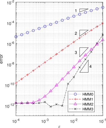
(a) Different $\varepsilon$ and fixed $\Delta t$

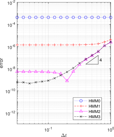
(b) Different $\Delta t$ and fixed $\varepsilon$

Figure 1: Numerical results for Example 6.2.

Example 6.3.

Forced Van der Pol equation [16]:

$$\left\{\begin{aligned} &\dfrac{\mathrm{d}x^{(1)}}{\mathrm{d}t}=-y+a\sin(2\pi x^{(2)}),\\ &\dfrac{\mathrm{d}x^{(2)}}{\mathrm{d}t}=b,\\ &\dfrac{\mathrm{d}y}{\mathrm{d}t}=\frac{1}{\varepsilon}\left(y+x^{(1)}-\frac{1}{3}y^{3}\right),\\ &x|_{t=0}=(x^{(1)},x^{(2)})|_{t=0}=x_{0},\ y|_{t=0}=y_{0},\end{aligned}\right.$$

with $x_{0}=(3,1)$, $y_{0}=1$, $a=2$, $b=1$, $T=1$.

Parameters: $\tau={1.0\times 10^{-6}}$, $M=25$, $\alpha=0.1$, $\Delta t_{c}={1.0\times 10^{-5}}$, $\hat{\beta}=0.01$.

Algorithm 2 and the forward difference formula are adopted. The reference solution is given by the coupled solver with time step size $\Delta t_{c}$. See Fig. 2(a) for fixed $\Delta t={1.0\times 10^{-2}}$ and different $\varepsilon$. See Fig. 2(b) for fixed $\varepsilon={1.0\times 10^{-4}}$ and different $\Delta t$.

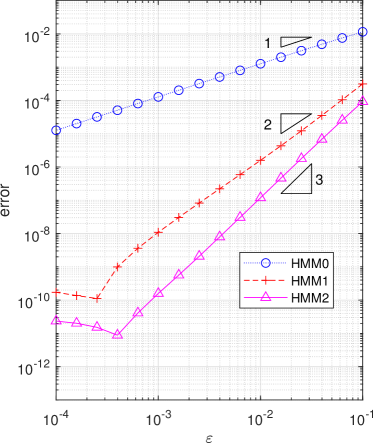
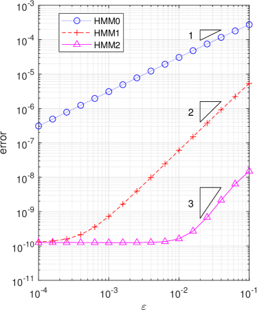
(a) Different $\varepsilon$ and fixed $\Delta t$

(b) Different $\Delta t$ and fixed $\varepsilon$

Figure 2: Numerical results for Example 6.3.

Example 6.4.

Cubic Chua’s model [7]:

$$\left\{\begin{aligned} &\dfrac{\mathrm{d}x^{(1)}}{\mathrm{d}t}=-dx^{(2)},\\ &\dfrac{\mathrm{d}x^{(2)}}{\mathrm{d}t}=-ay+x^{(1)}+bx^{(2)},\\ &\dfrac{\mathrm{d}y}{\mathrm{d}t}=\frac{1}{\varepsilon}(x^{(2)}-c_{3}y^{3}-c_{2}y^{2}-c_{1}y),\\ &x|_{t=0}=(x^{(1)},x^{(2)})|_{t=0}=x_{0},\ y|_{t=0}=y_{0},\end{aligned}\right.$$

with $x_{0}=(1,1)$, $y_{0}=1$, $a=0.7$, $b=0.25$, $c_{1}=7$, $c_{2}=15$, $c_{3}=20$, $d=1$, $T=1$.

Parameters: $\tau={1.0\times 10^{-6}}$, $M=10$, $\alpha=0.1$, $\Delta t_{c}={1.0\times 10^{-6}}$, $\hat{\beta}=10$.

Algorithm 2 and the central difference formula are adopted. The reference solution is given by the coupled solver with time step size $\Delta t_{c}$. See Fig. 3(a) for fixed $\Delta t={1.0\times 10^{-2}}$ and different $\varepsilon$. See Fig. 3(b) for fixed $\varepsilon={1.0\times 10^{-2}}$ and different $\Delta t$.

(a) Different $\varepsilon$ and fixed $\Delta t$

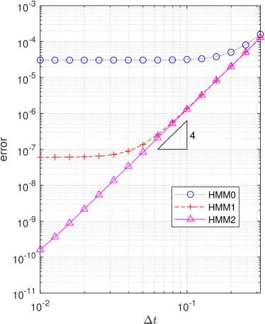
(b) Different $\Delta t$ and fixed $\varepsilon$

Figure 3: Numerical results for Example 6.4.

The results in Figs. 1(a), 2(a), and 3(a) show the order of numerical error. By numerical investigation, the theoretical result that the modeling error of HMM$k$ is of order $\mathcal{O}(\varepsilon^{k+1})$ is verified. The results in Figs. 1(b), 2(b), and 3(b) indicate whether the modeling error or the truncation error of macroscopic solver takes a dominant position in the numerical error.

6.3 Numerical derivative

It has been proven that the sampling error generated by numerical derivatives is $\mathcal{O}(\varepsilon\tau)$, if the forward difference formula is adopted. As seen in Remark 5.3, when the central difference formula is adopted, this part of error turns out to be $\mathcal{O}(\varepsilon\tau^{2})$. Let us consider the following numerical example.

Example 6.5.

Van der Pol equation [30, 12]:

$$\left\{\begin{aligned} &\dfrac{\mathrm{d}x}{\mathrm{d}t}=y,\\ &\dfrac{\mathrm{d}y}{\mathrm{d}t}=-\frac{1}{\varepsilon}\left((x^{2}-1)y+x\right),\\ &x|_{t=0}=x_{0},\ y|_{t=0}=y_{0},\end{aligned}\right.$$

with $x_{0}=4$, $y_{0}=2$, $T=5$.

Parameters: $M=20$, $\alpha=0.1$, $\Delta t_{c}=1.0\times 10^{-5}$, $\Delta t={2.0\times 10^{-2}}$, $\hat{\beta}=3$.

Algorithm 2 is adopted. The reference solution is given by the coupled solver with time step size $\Delta t_{c}$. We test the numerical error for different $\tau$ and different $\varepsilon$. See Fig. 4(a) for the forward difference formula. See Fig. 4(b) for the central difference formula.

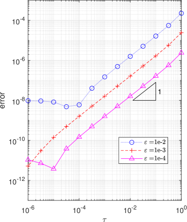
(a) Forward difference formula

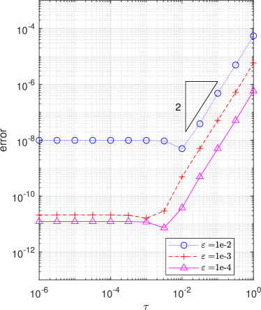
(b) Central difference formula

Figure 4: Numerical results for Example 6.5.

From the numerical results, one can see that, when $\tau$ is relatively large, the numerical error is approximately $\mathcal{O}(\varepsilon\tau)$ for the forward difference formula, and $\mathcal{O}(\varepsilon\tau^{2})$ for the central difference formula. Therefore, the theoretical analysis in Section 5.1 is verified.

7 Conclusions

We proposed a high-order numerical homogenization method for the dissipative ordinary differential equations. We develop the correction models based on the asymptotic approximations and a novel iterative formula. The corresponding numerical algorithms are designed in the framework of the heterogeneous multiscale methods. We provide some theoretical analysis on our algorithms. By numerical investigation, not only the error estimates are verified, but also the efficiency of our methods is exhibited.

Appendix A Well-posedness of Eq. 11 for Small $\varepsilon$

Theorem A.1.

Under the assumptions in Example 3.3, for each $M>\left\|A_{22}^{-1}A_{21}\right\|$, there exists $\delta\in(0,\varepsilon_{0}]$, such that for each $\varepsilon\in(0,\delta]$, there exists a unique solution $(C^{*},d^{*})$ to Eq. 11 such that $\left\|C^{*}\right\|\leq M$. Furthermore, $C^{*}+A_{22}^{-1}A_{21}=\mathcal{O}(\varepsilon)$ and $d^{*}+A_{22}^{-1}b_{2}=\mathcal{O}(\varepsilon)$.

Proof A.2.

First, we consider the equation Eq. 11a. It is easy to see that the solution of Eq. 11a is the fixed point of the mapping

$$\mathcal{T}:C\mapsto-A_{22}^{-1}A_{21}+\varepsilon A_{22}^{-1}CA_{11}+\varepsilon A_{22}^{-1}CA_{12}C.$$

We define a set $\mathcal{E}=\{C\in\mathbb{R}^{n_{y}\times n_{x}}:\left\|C\right\|\leq M\}$, where $M>\left\|A_{22}^{-1}A_{21}\right\|$ is arbitrary. Let $M_{1}=\left\|A_{22}^{-1}\right\|(\left\|A_{11}\right\|+\left\|A_{12}\right\|)$. When $C\in\mathcal{E}$, we have that

$$\left\|\mathcal{T}C\right\|\leq\left\|A_{22}^{-1}A_{21}\right\|+\varepsilon M_{1}\left\|C\right\|+\varepsilon M_{1}\left\|C\right\|^{2}\leq\left\|A_{22}^{-1}A_{21}\right\|+\varepsilon M_{1}(M+M^{2}).$$

We take $\delta_{1}=\min\left\{\varepsilon_{0},\frac{M-\left\|A_{22}^{-1}A_{21}\right\|}{M_{1}(M+M^{2})}\right\}>0$. For each $\varepsilon\in(0,\delta_{1}]$, we have that $\mathcal{T}:\mathcal{E}\rightarrow\mathcal{E}$. For each $C,\tilde{C}\in\mathcal{E}$,

$$\left\|\mathcal{T}C-\mathcal{T}\tilde{C}\right\| =\left\|\varepsilon A_{22}^{-1}(C-\tilde{C})A_{11}+\varepsilon A_{22}^{-1}(C-\tilde{C})A_{12}C+\varepsilon A_{22}^{-1}\tilde{C}A_{12}(C-\tilde{C})\right\|$$

$$\leq\varepsilon M_{1}(1+2M)\left\|C-\tilde{C}\right\|.$$

We take $\delta_{2}=\min\{\delta_{1},\frac{1}{2M_{1}(1+2M)}\}>0$. Then for each $\varepsilon\in(0,\delta_{2}]$, $\mathcal{T}$ is a contraction mapping on $\mathcal{E}$. Therefore, there exists a unique solution $C^{*}$ to Eq. 11a in $\mathcal{E}$. We take $\delta=\min\{\delta_{2},\frac{1}{2M_{1}M}\}$. For each $\varepsilon\in(0,\delta]$, $\left\|\varepsilon A_{22}^{-1}C^{*}A_{12}\right\|\leq\varepsilon M_{1}M\leq\frac{1}{2}<1$. Thus, $A_{22}-\varepsilon C^{*}A_{12}$ is invertible. With $C^{*}$ fixed, there exists a unique solution $d^{*}$ to Eq. 11b in $\mathbb{R}^{n_{y}}$, and $d^{*}$ is uniformly bounded in $\varepsilon\in(0,\delta]$. Furthermore, we notice that

$$C^{*}+A_{22}^{-1}A_{21}=\varepsilon(A_{22}^{-1}C^{*}A_{11}+A_{22}^{-1}C^{*}A_{12}C^{*})=\mathcal{O}(\varepsilon),$$

$$d^{*}+A_{22}^{-1}b_{2}=\varepsilon(A_{22}^{-1}C^{*}A_{12}d^{*}+A_{22}^{-1}C^{*}b_{1})=\mathcal{O}(\varepsilon).$$

Then the proof is completed.

Appendix B Proof of Theorem 3.11

Proof B.1 (Proof of Theorem 3.11).

By Remark 2.1, one can obtain that

$$|\Gamma_{1}(x,\varepsilon)-\gamma(x)-\varepsilon\gamma_{1}(x)| \leq\frac{1}{\beta}|g(x,\Gamma_{1}(x,\varepsilon))-g(x,\gamma(x)+\varepsilon\gamma_{1}(x))|$$

$$=\frac{1}{\beta}|\varepsilon\nabla\gamma(x)f(x,\gamma(x))-g(x,\gamma(x)+\varepsilon\gamma_{1}(x))|.$$

By Eq. 15b and Taylor’s expansion of $g(x,y)$ at $(x,\gamma(x))$,

$$\varepsilon\nabla\gamma(x)f(x,\gamma(x))-g(x,\gamma(x)+\varepsilon\gamma_{1}(x))$$

$$= \varepsilon G_{y}(x)\gamma_{1}(x)-\big{(}g(x,\gamma(x))+\varepsilon G_{y}(x)\gamma_{1}(x)+\mathcal{O}(\varepsilon^{2})\big{)}$$

$$= \mathcal{O}(\varepsilon^{2}),$$

where $\mathcal{O}(\varepsilon^{2})$ can be controlled uniformly thanks to Section 2.1. In other words, there exists a constant $C_{1}>0$ such that $|\varepsilon\nabla\gamma(x)f(x,\gamma(x))-g(x,\gamma(x)+\varepsilon\gamma_{1}(x))|\leq C_{1}\varepsilon^{2}$. Therefore,

$$|\Gamma_{1}(x,\varepsilon)-\gamma(x)-\varepsilon\gamma_{1}(x)|\leq\frac{C_{1}}{\beta}\varepsilon^{2},$$

which completes the proof of Eq. 20a.

By the expression of $\gamma_{1}(x)$ in Eq. 15b, one gets that

(34) $$g(x,\Gamma_{1}(x,\varepsilon))=\varepsilon G_{y}(x)\gamma_{1}(x).$$

For the sake of clarity, we consider the $i$-th component of Eq. 34, that is,

(35) $$g^{i}(x,\Gamma_{1}(x,\varepsilon))=\varepsilon\sum_{k=1}^{n_{y}}\frac{\partial g^{i}}{\partial y^{k}}(x,\gamma(x))\gamma_{1}^{k}(x).$$

Taking the derivative of Eq. 35 with respect to $x^{j}$, we obtain that

(36) $$\frac{\partial g^{i}}{\partial x^{j}}(x,\Gamma_{1}(x,\varepsilon))+\sum_{k=1}^{n_{y}}\frac{\partial g^{i}}{\partial y^{k}}(x,\Gamma_{1}(x,\varepsilon))\frac{\partial\Gamma_{1}^{k}}{\partial x^{j}}(x,\varepsilon)$$

$$= \varepsilon\sum_{k=1}^{n_{y}}\bigg{(}\frac{\partial^{2}g^{i}}{\partial y^{k}\partial x^{j}}(x,\gamma(x))+\sum_{\ell=1}^{n_{y}}\frac{\partial^{2}g^{i}}{\partial y^{k}\partial y^{\ell}}(x,\gamma(x))\frac{\partial\gamma^{\ell}}{\partial x^{j}}(x)\bigg{)}\gamma_{1}^{k}(x)$$

$$\quad\quad+\varepsilon\sum_{k=1}^{n_{y}}\frac{\partial g^{i}}{\partial y^{k}}(x,\gamma(x))\frac{\partial\gamma_{1}^{k}}{\partial x^{j}}(x).$$

Actually Eq. 36 yields that $\nabla_{x}\Gamma_{1}(x,\varepsilon)$ is uniformly bounded in $\varepsilon\in(0,\varepsilon_{0}]$, since

$$\nabla_{x}\Gamma_{1}(x,\varepsilon)=G_{y}(x)^{-1}A,$$

where $A=A(x,\varepsilon)=[A^{i,j}]_{i=1,j=1}^{n_{y},n_{x}}$, $A^{i,j}$ is defined as

$$A^{i,j} =\varepsilon\sum_{k=1}^{n_{y}}\bigg{(}\frac{\partial^{2}g^{i}}{\partial y^{k}\partial x^{j}}(x,\gamma(x))+\sum_{\ell=1}^{n_{y}}\frac{\partial^{2}g^{i}}{\partial y^{k}\partial y^{\ell}}(x,\gamma(x))\frac{\partial\gamma^{\ell}}{\partial x^{j}}(x)\bigg{)}\gamma_{1}^{k}(x)$$

$$\quad\quad\quad+\varepsilon\sum_{k=1}^{n_{y}}\frac{\partial g^{i}}{\partial y^{k}}(x,\gamma(x))\frac{\partial\gamma_{1}^{k}}{\partial x^{j}}(x)-\frac{\partial g^{i}}{\partial x^{j}}(x,\Gamma_{1}(x,\varepsilon)),$$

and it is obvious that $A(x,\varepsilon)$ is uniformly bounded in $\varepsilon\in(0,\varepsilon_{0}]$ due to Section 2.1. By Eq. 20a and Taylor’s expansion of $\frac{\partial g^{i}}{\partial x^{j}}$ and $\frac{\partial g^{i}}{\partial y^{k}}$ at $(x,\gamma(x))$, one obtains that

(37) $$\frac{\partial g^{i}}{\partial x^{j}}(x,\Gamma_{1}(x,\varepsilon))=\frac{\partial g^{i}}{\partial x^{j}}(x,\gamma(x))+\varepsilon\sum_{k=1}^{n_{y}}\frac{\partial^{2}g^{i}}{\partial x^{j}\partial y^{k}}(x,\gamma(x))\gamma_{1}^{k}(x)+\mathcal{O}(\varepsilon^{2}),$$

and

(38) $$\frac{\partial g^{i}}{\partial y^{k}}(x,\Gamma_{1}(x,\varepsilon))=\frac{\partial g^{i}}{\partial y^{k}}(x,\gamma(x))+\varepsilon\sum_{\ell=1}^{n_{y}}\frac{\partial^{2}g^{i}}{\partial y^{k}\partial y^{\ell}}(x,\gamma(x))\gamma_{1}^{\ell}(x)+\mathcal{O}(\varepsilon^{2}),$$

where both $\mathcal{O}(\varepsilon^{2})$ can be controlled uniformly due to Section 2.1. In addition, the $(i,j)$-component of Eq. 16 can be written as

(39) $$\frac{\partial g^{i}}{\partial x^{j}}(x,\gamma(x))=-\sum_{k=1}^{n_{y}}\frac{\partial g^{i}}{\partial y^{k}}(x,\gamma(x))\frac{\partial\gamma^{k}}{\partial x^{j}}(x).$$

By Eq. 36, Eq. 37, Eq. 38, Eq. 39 and the uniform boundedness of $\nabla_{x}\Gamma_{1}(x,\varepsilon)$, one can obtain that

(40) $$\sum_{k=1}^{n_{y}}\bigg{(}\frac{\partial g^{i}}{\partial y^{k}}(x,\gamma(x))+\varepsilon B^{i,k}\bigg{)}\cdot\bigg{(}\frac{\partial\Gamma_{1}^{k}}{\partial x^{j}}(x,\varepsilon)-\frac{\partial\gamma^{k}}{\partial x^{j}}(x)-\varepsilon\frac{\partial\gamma_{1}^{k}}{\partial x^{j}}(x)\bigg{)}=\mathcal{O}(\varepsilon^{2}),$$

where $\mathcal{O}(\varepsilon^{2})$ can be controlled uniformly, $B=B(x)=[B^{i,k}]_{i,k=1}^{n_{y}}$ defined as

$$B^{i,k}=\sum_{\ell=1}^{n_{y}}\frac{\partial^{2}g^{i}}{\partial y^{k}\partial y^{\ell}}(x,\gamma(x))\gamma_{1}^{\ell}(x).$$

Eq. 40 can be rewritten as

(41) $$(G_{y}(x)+\varepsilon B)(\nabla_{x}\Gamma_{1}(x,\varepsilon)-\nabla\gamma(x)-\varepsilon\nabla\gamma_{1}(x))=\mathcal{O}(\varepsilon^{2}).$$

Notice that $B(x)$ is uniformly bounded thanks to Section 2.1. Therefore, as long as $\varepsilon$ is sufficiently small, $G_{y}(x)+\varepsilon B$ is invertible and $(G_{y}(x)+\varepsilon B)^{-1}$ is uniformly bounded. Therefore, the proof of Eq. 20b is completed by Eq. 41.

By Remark 2.1, one obtains that

$$|\Gamma_{2}(x,\varepsilon)-\gamma(x)-\varepsilon\gamma_{1}(x)-\varepsilon^{2}\gamma_{2}(x)|$$

$$\leq \frac{1}{\beta}|g(x,\Gamma_{2}(x,\varepsilon))-g(x,\gamma(x)+\varepsilon\gamma_{1}(x)+\varepsilon^{2}\gamma_{2}(x))|$$

$$\leq \frac{1}{\beta}|\varepsilon\nabla_{x}\Gamma_{1}(x,\varepsilon)f(x,\Gamma_{1}(x,\varepsilon))-g(x,\gamma(x)+\varepsilon\gamma_{1}(x)+\varepsilon^{2}\gamma_{2}(x))|.$$

By Eq. 20a, Eq. 20b and Taylor’s expansion of $f(x,y)$ at $(x,\gamma(x))$, one gets that

(42) $$\varepsilon\nabla_{x}\Gamma_{1}(x,\varepsilon)f(x,\Gamma_{1}(x,\varepsilon))$$

$$= \varepsilon\big{(}\nabla\gamma(x)+\varepsilon\nabla\gamma_{1}(x)\big{)}\big{(}F(x)+\varepsilon F_{y}(x)\gamma_{1}(x)\big{)}+\mathcal{O}(\varepsilon^{3})$$

$$= \varepsilon\nabla\gamma(x)F(x)+\varepsilon^{2}\big{(}\nabla\gamma(x)F_{y}(x)\gamma_{1}(x)+\nabla\gamma_{1}(x)F(x)\big{)}+\mathcal{O}(\varepsilon^{3}).$$

By Taylor’s expansion of $g(x,y)$ at $(x,\gamma(x))$, one gets that

(43) $$g(x,\gamma(x)+\varepsilon\gamma_{1}(x)+\varepsilon^{2}\gamma_{2}(x))$$

$$= \varepsilon G_{y}(x)\gamma_{1}(x)+\varepsilon^{2}\Bigg{(}G_{y}(x)\gamma_{2}(x)+\frac{1}{2}\Big{[}\sum_{j,k=1}^{n_{y}}G_{yy}^{i,j,k}\gamma_{1}^{j}(x)\gamma_{1}^{k}(x)\Big{]}_{i=1}^{n_{y}}\Bigg{)}+\mathcal{O}(\varepsilon^{3}).$$

By comparing Eq. 42 and Eq. 43, one obtains that

$$|\varepsilon\nabla_{x}\Gamma_{1}(x,\varepsilon)f(x,\Gamma_{1}(x,\varepsilon))-g(x,\gamma(x)+\varepsilon\gamma_{1}(x)+\varepsilon^{2}\gamma_{2}(x))|=\mathcal{O}(\varepsilon^{3}),$$

where $\mathcal{O}(\varepsilon^{3})$ can be controlled uniformly thanks to Section 2.1. In other words, there exists a constant $C_{2}>0$ such that $|\varepsilon\nabla_{x}\Gamma_{1}(x,\varepsilon)f(x,\Gamma_{1}(x,\varepsilon))-g(x,\gamma(x)+\varepsilon\gamma_{1}(x)+\varepsilon^{2}\gamma_{2}(x))|\leq C_{2}\varepsilon^{3}$. Therefore,

$$|\Gamma_{2}(x,\varepsilon)-\gamma(x)-\varepsilon\gamma_{1}(x)-\varepsilon^{2}\gamma_{2}(x)|\leq\frac{C_{2}}{\beta}\varepsilon^{3}.$$

Thus, the proof for Eq. 20c is completed.

Appendix C Proofs of Theorems 3.12, 3.13, and 5.1

C.1 Several lemmas

In the proofs of these three theorems, we have to calculate high-order gradients of vector-valued functions. Here we present several facts about high-order derivatives.

Lemma C.1.

Suppose that the functions $A$, $\xi$, $\eta$ in this lemma are sufficiently smooth. We have the following conclusions.

1. Assume that $k\geq 0$ and $\xi,\eta\in W^{k,\infty}(\mathbb{R}^{n},\mathbb{R})$, then

   $$|\xi\eta|_{k,\infty}\lesssim\sum_{j=0}^{k}|\xi|_{j,\infty}|\eta|_{k-j,\infty}.$$

   where the bound is dependent on $k$, and independent of $\xi$ and $\eta$.

2. Assume that $k\geq 0$. Let $\xi:\mathbb{R}^{n}\rightarrow\mathbb{R}$ and $\eta:\mathbb{R}^{m}\rightarrow\mathbb{R}^{n}$ be sufficiently smooth functions. If $\nabla\xi\in W^{k,\infty}$ and $\nabla\eta\in W^{k,\infty}$, then

   $$|\xi\circ\eta|_{k+1,\infty}\lesssim\sum_{j=1}^{k+1}|\xi|_{j,\infty}\left\|\nabla\eta\right\|_{k+1-j,\infty}^{j},$$

   where the bound is dependent on $k$, and independent of $\xi$ and $\eta$. In particular, if $\xi\in W^{k+1,\infty}$ and $\nabla\eta\in W^{k,\infty}$, then $\xi\circ\eta\in W^{k+1,\infty}$.

3. Assume that $k\geq 0$. Let $A:\mathbb{R}^{m}\rightarrow\mathbb{R}^{n\times n}$ is a matrix-valued function. If $\nabla A\in W^{k,\infty}$ and $A(\cdot)^{-1}\in\mathcal{L}^{\infty}$, then

   $$|A(\cdot)^{-1}|_{k+1,\infty}\lesssim\sum_{j=1}^{k+1}\left\|A(\cdot)^{-1}\right\|_{0,\infty}^{j+1}\left\|\nabla A\right\|_{k+1-j,\infty}^{j},$$

   where the bound is dependent on $k$, and independent of $A$.

Proof C.2.

Item 1 is a direct corollary of Leibniz rule.

As for Item 2, first we notice that

$$\nabla_{x}\left((\xi\circ\eta)(x)\right)=\left((\nabla\xi)\circ\eta\right)(x)\cdot\nabla\eta(x),$$

which yields directly that the conclusion holds for $k=0$. Now we assume that the conclusion holds for all non-negative integers that are less than $k$, and then one can obtain by Item 1 and the induction hypothesis that

$$|\xi\circ\eta|_{k+2,\infty} =\left|\big{(}(\nabla\xi)\circ\eta\big{)}\cdot\nabla\eta\right|_{k+1,\infty}$$

$$\lesssim\sum_{i=0}^{k+1}\left|(\nabla\xi)\circ\eta\right|_{i,\infty}|\nabla\eta|_{k+1-i,\infty}$$

$$\lesssim|\xi|_{1,\infty}|\nabla\eta|_{k+1,\infty}+\sum_{i=1}^{k+1}\sum_{j=1}^{i}|\xi|_{j+1,\infty}\left\|\nabla\eta\right\|_{i-j,\infty}^{j}|\nabla\eta|_{k+1-i,\infty}$$

$$\leq|\xi|_{1,\infty}|\nabla\eta|_{k+1,\infty}+\sum_{j=1}^{k+1}\sum_{i=j}^{k+1}|\xi|_{j+1,\infty}\left\|\nabla\eta\right\|_{k+1-j,\infty}^{j+1}$$

$$\lesssim\sum_{j=1}^{k+2}|\xi|_{j,\infty}\left\|\nabla\eta\right\|_{k+2-j,\infty}^{j},$$

which completes the proof.

As for Item 3, one can notice first that $A(x)^{-1}$ is continuous, which yields that

$$\dfrac{\partial A(x)^{-1}}{\partial x^{i}}=-A(x)^{-1}\dfrac{\partial A(x)}{\partial x^{i}}A(x)^{-1},\ \forall i=1,2,\ldots,m.$$

Then the conclusion can be proved similarly to Item 2.

Lemma C.3.

Suppose that $\Phi:\mathbb{R}^{n}\times[-\delta,\delta]\rightarrow\mathbb{R}$ is sufficiently smooth. If there exists $k,\ell\in\mathbb{N}$ such that the function $\Phi(x,s)$ satisfies

$$\dfrac{\partial^{i}\Phi}{\partial s^{i}}(x,0)=0,\ \forall i=0,1,\ldots,\ell,$$

and

$$\sup_{s\in[-\delta,\delta]}\left\|\dfrac{\partial^{\ell+1}\Phi}{\partial s^{\ell+1}}(\cdot,s)\right\|_{k,\infty}<+\infty,$$

then

$$\left\|\Phi(\cdot,h)\right\|_{k,\infty}=\mathcal{O}(|h|^{\ell+1}),\text{ as }h\rightarrow 0.$$

Proof C.4.

By Taylor’s expansion, for each $j=0,1,\ldots,k$, there exists $\theta\in[0,1]$ such that

$$|\nabla_{x}^{j}\Phi(x,h)|=\frac{1}{(\ell+1)!}\left|\nabla_{x}^{j}\dfrac{\partial^{\ell+1}\Phi}{\partial s^{\ell+1}}(x,\theta h)h^{\ell+1}\right|\lesssim\sup_{s\in[-\delta,\delta]}\left\|\dfrac{\partial^{\ell+1}\Phi}{\partial s^{\ell+1}}(\cdot,s)\right\|_{k,\infty}|h|^{\ell+1},$$

which completes the proof.

Corollary C.5.

Suppose that $\xi:\mathbb{R}^{n}\rightarrow\mathbb{R}$ and $\eta:\mathbb{R}^{n}\rightarrow\mathbb{R}^{n}$ are sufficiently smooth, and $\eta\in W^{k,\infty}$. We have the following conclusions.

1. If $\nabla^{2}\xi\in W^{k,\infty}$, then

   $$\left\|\xi(\cdot+\eta(\cdot)h)-\xi(\cdot)-h\nabla\xi(\cdot)\eta(\cdot)\right\|_{k,\infty}=\mathcal{O}(|h|^{2}),\text{ as }h\rightarrow 0.$$

2. If $\nabla^{3}\xi\in W^{k,\infty}$, then

   $$\left\|\xi(\cdot+\eta(\cdot)h)-\xi(\cdot-\eta(\cdot)h)-2h\nabla\xi(\cdot)\eta(\cdot)\right\|_{k,\infty}=\mathcal{O}(|h|^{3}),\text{ as }h\rightarrow 0.$$

Proof C.6.

Let $\Phi(x,s)=\xi(x+\eta(x)s)-\xi(x)-s\nabla\xi(x)\eta(x)$. By direct calculation, one can obtain that

$$\dfrac{\partial\Phi}{\partial s}(x,s)=\nabla\xi\big{(}x+\eta(x)s\big{)}\eta(x)-\nabla\xi(x)\eta(x),$$

$$\dfrac{\partial^{2}\Phi}{\partial s^{2}}(x,s)=\sum_{i_{1},i_{2}=1}^{n}\dfrac{\partial^{2}\xi}{\partial x^{i_{1}}\partial x^{i_{2}}}\big{(}x+\eta(x)s\big{)}\eta^{i_{1}}(x)\eta^{i_{2}}(x),$$

$$\dfrac{\partial^{3}\Phi}{\partial s^{3}}(x,s)=\sum_{i_{1},i_{2},i_{3}=1}^{n}\dfrac{\partial^{3}\xi}{\partial x^{i_{1}}\partial x^{i_{2}}\partial x^{i_{3}}}\big{(}x+\eta(x)s\big{)}\eta^{i_{1}}(x)\eta^{i_{2}}(x)\eta^{i_{3}}(x).$$

Notice that $\Phi(x,0)=\dfrac{\partial\Phi}{\partial s}(x,0)=0$. By Lemma C.1, $\Phi(x,s)$ satisfies the conditions of Lemma C.3 when $\ell=1$, which yields Item 1. Similarly, $\Phi(x,s)-\Phi(x,-s)$ satisfies Lemma C.3 when $\ell=2$, which completes the proof.

Lemma C.7.

If $z_{0},z_{1}\in\mathcal{C}^{k}(\mathbb{R}^{n_{x}},\mathbb{R}^{n_{y}})$ for some $k=1,2,\ldots,K$, then there exist unique $y_{0},y_{1}\in\mathcal{C}^{k}(\mathbb{R}^{n_{x}},\mathbb{R}^{n_{y}})$ satisfying that $g(x,y_{i}(x))=z_{i}(x)$ for $i=0,1$. In addition, if $z_{i}\in W^{k,\infty}$ for $i=0,1$, then

$$\left\|y_{1}-y_{0}\right\|_{k,\infty}\lesssim\left\|z_{1}-z_{0}\right\|_{k,\infty},$$

where the bound is dependent on $\beta$, $k$ and $\left\|z_{i}\right\|_{k,\infty}$ where $i=0,1$.

Proof C.8.

By Remark 2.1 and implicit function theorem for $g(x,y)-sz_{1}(x)-(1-s)z_{0}(x)=0$ with respect to $y$, there exists a unique function $y=y(x,s)\in\mathcal{C}^{k}(\mathbb{R}^{n_{x}}\times[0,1],\mathbb{R}^{n_{y}})$ such that

(44) $$g(x,y(x,s))=sz_{1}(x)+(1-s)z_{0}(x).$$

Now we assume that $z_{i}\in W^{k,\infty}$ for $i=0,1$. Let $y_{i}(x)=y(x,i)$ for $i=0,1$. For each $j=0,1,\ldots,k$, there exists $\theta\in[0,1]$ such that

(45) $$|\nabla^{j}y_{1}(x)-\nabla^{j}y_{0}(x)|\leq\left|\dfrac{\partial}{\partial s}\nabla^{j}_{x}y(x,\theta)\right|.$$

By Eq. 44, one obtains that

(46) $$\dfrac{\partial y}{\partial s}(x,s)=\left(\dfrac{\partial g}{\partial y}(x,y(x,s))\right)^{-1}(z_{1}(x)-z_{0}(x))$$

and

(47) $$\nabla_{x}y(x,s)=\left(\dfrac{\partial g}{\partial y}(x,y(x,s))\right)^{-1}\left(s\nabla z_{1}(x)+(1-s)\nabla z_{0}(x)-\dfrac{\partial g}{\partial x}(x,y(x,s))\right).$$

We assert that $\sup\limits_{s\in[0,1]}\left\|\nabla_{x}y(\cdot,s)\right\|_{k-1,\infty}$ is bounded, where the bound is dependent on $\beta$, $k$ and $\left\|z_{i}\right\|_{k,\infty}$. By Eq. 47, $\sup\limits_{s\in[0,1]}\left\|\nabla_{x}y(\cdot,s)\right\|_{0,\infty}$ is bounded. Now assume that $\sup\limits_{s\in[0,1]}\left\|\nabla_{x}y(\cdot,s)\right\|_{j,\infty}$ is bounded for some $j=0,1,\ldots,k-2$. Lemma C.1 yields that $\sup\limits_{s\in[0,1]}\left\|\dfrac{\partial g}{\partial(x,y)}(\cdot,y(\cdot,s))\right\|_{j+1,\infty}$ and then $\sup\limits_{s\in[0,1]}\left\|\nabla_{x}y(\cdot,s)\right\|_{j+1,\infty}$ are bounded, which yields the assertion.

By the above assertion and Lemma C.1, $\left(\dfrac{\partial g}{\partial y}(x,y(x,s))\right)^{-1}$ is bounded in $W^{k,\infty}$, where the bound depends on $\beta$, $k$ and $\left\|z_{i}\right\|_{k,\infty}$. Therefore, by Eq. 46, one obtains that

$$\sup_{s\in[0,1]}\left\|\dfrac{\partial y}{\partial s}(\cdot,s)\right\|_{k,\infty}\lesssim\left\|z_{1}-z_{0}\right\|_{k,\infty}.$$

Together with Eq. 45, the proof is completed.

Lemma C.9.

Assume that $y_{i}:\mathbb{R}^{n_{x}}\rightarrow\mathbb{R}^{n_{y}}$ satisfies that $y_{i}\in\mathcal{C}^{k+1}$ and $\nabla y_{i}\in W^{k,\infty}$ for each $i=0,1$ and some $k=0,1,\ldots,K-1$. If $y_{1}-y_{0}\in\mathcal{L}^{\infty}$, then

$$\left\|\nabla y_{1}(\cdot)f(\cdot,y_{1}(\cdot))-\nabla y_{0}(\cdot)f(\cdot,y_{0}(\cdot))\right\|_{k,\infty}\lesssim\left\|y_{1}-y_{0}\right\|_{k+1,\infty},$$

where the bound depends on $f$, $k$ and $\left\|\nabla y_{i}\right\|_{k,\infty}$ with $i=0,1$.

Proof C.10.

Let $\Phi(x,s)=sy_{1}(x)+(1-s)y_{0}(x)$ and $\Psi(x,s)=\nabla_{x}\Phi(x,s)f(x,\Phi(x,s))$. For each $j=0,1,\ldots,k$, there exists $\theta\in[0,1]$ such that

$$|\nabla_{x}^{j}\Psi(x,1)-\nabla_{x}^{j}\Psi(x,0)|\leq\left|\dfrac{\partial}{\partial s}\nabla_{x}^{j}\Psi(x,\theta)\right|.$$

Actually,

(48) $$\dfrac{\partial\Psi}{\partial s}(x,s) =\nabla_{x}\left(\dfrac{\partial\Phi}{\partial s}(x,s)\right)f(x,\Phi(x,s))+\nabla_{x}\Phi(x,s)\dfrac{\partial f}{\partial y}(x,\Phi(x,s))\dfrac{\partial\Phi}{\partial s}(x,s)$$

$$=(\nabla y_{1}(x)-\nabla y_{0}(x))f(x,\Phi(x,s))+\nabla_{x}\Phi(x,s)\dfrac{\partial f}{\partial y}(x,\Phi(x,s))(y_{1}(x)-y_{0}(x)).$$

By Lemma C.1, one obtains that $\sup\limits_{s\in[0,1]}\left\|f(\cdot,\Phi(\cdot,s))\right\|_{k,\infty}$ and $\sup\limits_{s\in[0,1]}\left\|\nabla_{x}\Phi(\cdot,s)\dfrac{\partial f}{\partial y}(\cdot,\Phi(\cdot,s))\right\|_{k,\infty}$ are bounded, and the bound depends on $f$, $k$ and $\left\|\nabla y_{i}\right\|_{k,\infty}$ with $i=0,1$. Therefore,

$$\sup_{s\in[0,1]}\left\|\dfrac{\partial\Psi}{\partial s}(\cdot,s)\right\|_{k,\infty}\lesssim\left\|y_{1}-y_{0}\right\|_{k+1,\infty},$$

which completes the proof.

Corollary C.11.

For $k=0,1,\ldots,K$,

(49) $$\left\|\Gamma_{k+1}(\cdot,\varepsilon)-\Gamma_{k}(\cdot,\varepsilon)\right\|_{K-k,\infty}=\mathcal{O}(\varepsilon^{k+1}).$$

Proof C.12.

By Eq. 16 and Lemma C.1, one can prove by induction that $\left\|\nabla_{x}\Gamma_{0}(\cdot,\varepsilon)\right\|_{K,\infty}$ is bounded. Therefore, $\left\|\varepsilon\nabla_{x}\Gamma_{0}(\cdot,\varepsilon)f(\cdot,\Gamma_{0}(\cdot,\varepsilon))\right\|_{K,\infty}=\mathcal{O}(\varepsilon)$. By Lemma C.7, $\left\|\Gamma_{1}(\cdot,\varepsilon)-\Gamma_{0}(\cdot,\varepsilon)\right\|_{K,\infty}=\mathcal{O}(\varepsilon)$. Now assume that Eq. 49 holds for $0,1,\ldots,k$ where $k\leq K-1$. By the induction hypothesis, $\left\|\nabla_{x}\Gamma_{j}(\cdot,\varepsilon)\right\|_{K-k-1,\infty}$ are bounded for $j=0,1,\ldots,k+1$. By Lemma C.9, one obtains that

$$\left\|\nabla_{x}\Gamma_{k+1}(\cdot,\varepsilon)f(\cdot,\Gamma_{k+1}(\cdot,\varepsilon))-\nabla_{x}\Gamma_{k}(\cdot,\varepsilon)f(\cdot,\Gamma_{k}(\cdot,\varepsilon))\right\|_{K-k-1,\infty}=\mathcal{O}(\varepsilon^{k+1}).$$

By Lemma C.7, the proof is completed.

C.2 Proof of Theorem 3.12

Proof C.13 (Proof of Theorem 3.12).

We prove this theorem by induction.

When $k=0$, there exists a constant $C>0$ dependent on $k$ such that

$$\dfrac{\mathrm{d}|z_{0}|^{2}}{\mathrm{d}t} =\frac{2}{\varepsilon}\left\langle{z_{0}},{g(x,y)-g(x,\gamma(x))}\right\rangle-2\left\langle{z_{0}},{\nabla\gamma(x)f(x,y)}\right\rangle$$

$$\leq-\frac{2\beta}{\varepsilon}|z_{0}|^{2}+C|z_{0}|\leq-\frac{A}{\varepsilon}|z_{0}|^{2}+\frac{C^{2}}{4(2\beta-A)}\varepsilon.$$

Here the last inequality is due to Cauchy inequality. By Gronwall inequality,

$$|z_{0}(t)|^{2}\leq\frac{C^{2}}{A(2\beta-A)}\varepsilon^{2}(1-e^{-\frac{A}{\varepsilon}t})+e^{-\frac{A}{\varepsilon}t}|z_{0}(0)|^{2}\leq\frac{C^{2}}{A(2\beta-A)}\varepsilon^{2}+e^{-\frac{A}{\varepsilon}t}|z_{0}(0)|^{2}.$$

Assuming that the theorem holds for $k-1$, where $k=1,2,\ldots,K$. One obtains that

(50) $$\dfrac{\mathrm{d}|z_{k}|^{2}}{\mathrm{d}t} =\frac{2}{\varepsilon}\left\langle{z_{k}},{g(x,y)-g(x,\Gamma_{k}(x,\varepsilon))}\right\rangle$$

$$\quad\quad\quad+2\left\langle{z_{k}},{\nabla_{x}\Gamma_{k-1}(x,\varepsilon)f(x,\Gamma_{k-1}(x,\varepsilon))-\nabla_{x}\Gamma_{k}(x,\varepsilon)f(x,y)}\right\rangle$$

$$\leq-\frac{2\beta}{\varepsilon}|z_{k}|^{2}+2|z_{k}|\cdot|\nabla_{x}\Gamma_{k-1}(x,\varepsilon)f(x,\Gamma_{k-1}(x,\varepsilon))-\nabla_{x}\Gamma_{k}(x,\varepsilon)f(x,y)|.$$

Corollary C.11 and Section 2.1 yield that there exists a constant $C>0$ such that

(51) $$2|\nabla_{x}\Gamma_{k-1}(x,\varepsilon)f(x,\Gamma_{k-1}(x,\varepsilon))-\nabla_{x}\Gamma_{k}(x,\varepsilon)f(x,y)|$$

$$\leq 2|\nabla_{x}\Gamma_{k-1}(x,\varepsilon)f(x,\Gamma_{k-1}(x,\varepsilon))-\nabla_{x}\Gamma_{k}(x,\varepsilon)f(x,\Gamma_{k-1}(x,\varepsilon))|$$

$$\quad+2|\nabla_{x}\Gamma_{k}(x,\varepsilon)f(x,\Gamma_{k-1}(x,\varepsilon))-\nabla_{x}\Gamma_{k}(x,\varepsilon)f(x,y)|$$

$$\leq C\varepsilon^{k}+C|z_{k-1}|.$$

Take $\tilde{A}\in(A,2\beta)$. Combing Eq. 50 and Eq. 51, one gets by Cauchy inequality that

(52) $$\dfrac{\mathrm{d}|z_{k}|^{2}}{\mathrm{d}t} \leq-\frac{2\beta}{\varepsilon}|z_{k}|^{2}+C\varepsilon^{k}|z_{k}|+C|z_{k-1}|\cdot|z_{k}|$$

$$\leq-\frac{\tilde{A}}{\varepsilon}|z_{k}|^{2}+\frac{C^{2}}{2(2\beta-\tilde{A})}\varepsilon^{2k+1}+\frac{C^{2}}{2(2\beta-\tilde{A})}\varepsilon|z_{k-1}|^{2}.$$

The induction hypothesis says that there exists $C_{k-1}>0$ such that

(53) $$|z_{k-1}(t)|^{2}\leq C_{k-1}(\varepsilon^{2k}+e^{-\frac{\tilde{A}}{\varepsilon}t}|z_{k-1}(0)|^{2}).$$

By Eq. 52, Eq. 53 and Gronwall’s inequality, one gets that

(54) $$|z_{k}(t)|^{2} \leq\frac{C^{2}(1+C_{k-1})}{2\tilde{A}(2\beta-\tilde{A})}(1-e^{-\frac{\tilde{A}}{\varepsilon}t})\varepsilon^{2k+2}+e^{-\frac{\tilde{A}}{\varepsilon}t}|z_{k}(0)|^{2}+\frac{C^{2}C_{k-1}}{2(2\beta-\tilde{A})}te^{-\frac{\tilde{A}}{\varepsilon}t}\varepsilon|z_{k-1}(0)|^{2}$$

$$\leq\frac{C^{2}(1+C_{k-1})}{2\tilde{A}(2\beta-\tilde{A})}\varepsilon^{2k+2}+e^{-\frac{A}{\varepsilon}t}|z_{k}(0)|^{2}+\frac{C^{2}C_{k-1}e^{-1}}{2(\tilde{A}-A)(2\beta-\tilde{A})}e^{-\frac{A}{\varepsilon}t}\varepsilon^{2}|z_{k-1}(0)|^{2}.$$

By Corollary C.11, one gets that

(55) $$|z_{k-1}(0)|^{2}\leq 2|z_{k}(0)|^{2}+2|z_{k}(0)-z_{k-1}(0)|^{2}\leq 2|z_{k}(0)|^{2}+C\varepsilon^{2k}.$$

By Eq. 54 and Eq. 55, the theorem holds for $k$. Then the theorem is thus proved.

C.3 Proof of Theorem 3.13

Proof C.14 (Proof of Theorem 3.13).

Since $\nabla_{x}f(x,y)$, $\nabla_{y}f(x,y)$ and $\nabla_{x}\Gamma_{k}(x,\varepsilon)$ are all bounded, then there exists a constant $C>0$ such that

$$\left|\dfrac{\mathrm{d}(x-X_{k})}{\mathrm{d}t}\right|=|f(x,y)-f(X_{k},\Gamma_{k}(X_{k},\varepsilon))|$$

$$\leq |f(x,z_{k}+\Gamma_{k}(x,\varepsilon))-f(x,\Gamma_{k}(X_{k},\varepsilon))|+|f(x,\Gamma_{k}(X_{k},\varepsilon))-f(X_{k},\Gamma_{k}(X_{k},\varepsilon))|$$

$$\leq C|z_{k}|+C|x-X_{k}|.$$

Then one obtains that

$$\frac{1}{2}\dfrac{\mathrm{d}|x-X_{k}|^{2}}{\mathrm{d}t}=\left\langle{x-X_{k}},{\dfrac{\mathrm{d}(x-X_{k})}{\mathrm{d}t}}\right\rangle\leq|x-X_{k}|\cdot\left|\dfrac{\mathrm{d}(x-X_{k})}{\mathrm{d}t}\right|\leq C|z_{k}|\cdot|x-X_{k}|+C|x-X_{k}|^{2}.$$

Therefore, by Theorem 3.12 and Cauchy-Schwarz inequality, there exists a constant $C_{k}>0$ such that

$$\dfrac{\mathrm{d}|x-X_{k}|^{2}}{\mathrm{d}t}\leq C_{k}(|x-X_{k}|^{2}+\varepsilon^{2k+2}+e^{-\frac{\beta}{\varepsilon}t}|z_{k}(0)|^{2}).$$

By Gronwall inequality,

$$|x(t)-X_{k}(t)|^{2}\leq e^{C_{k}t}|x(0)-X_{k}(0)|^{2}+\varepsilon^{2k+2}(e^{C_{k}t}-1)+C_{k}\frac{e^{C_{k}t}-e^{-\frac{\beta}{\varepsilon}t}}{\frac{\beta}{\varepsilon}+C_{k}}|z_{k}(0)|^{2},$$

which completes the proof.

C.4 Proof of Theorem 5.1

Proof C.15 (Proof of Theorem 5.1).

When $k=0$, Eq. 33 is straightforward since $\Gamma_{0}(x,\varepsilon)=\hat{\Gamma}^{\mathrm{d}}_{0}(x,\varepsilon)$. Assume that Eq. 33 holds for $0,1,\ldots,k$ where $k=0,1,\ldots,\lfloor\frac{K}{2}\rfloor-1$. By Lemma C.7, it suffices to show that

(56) $$\left\|\hat{\Gamma}^{\mathrm{d}}_{k}(\cdot+f(\cdot,\hat{\Gamma}^{\mathrm{d}}_{k}(\cdot,\varepsilon))\tau,\varepsilon)-\hat{\Gamma}^{\mathrm{d}}_{k}(\cdot,\varepsilon)-\tau\nabla_{x}\Gamma_{k}(\cdot,\varepsilon)f(\cdot,\Gamma_{k}(\cdot,\varepsilon))\right\|_{K-2k-2,\infty}=\mathcal{O}(\tau^{2}).$$

By the induction hypothesis, $\left\|\nabla_{x}\hat{\Gamma}^{\mathrm{d}}_{k}(\cdot,\varepsilon)\right\|_{K-2k-1,\infty}$ is bounded. By Lemma C.9,

(57) $$\left\|\tau\nabla_{x}\hat{\Gamma}^{\mathrm{d}}_{k}(\cdot,\varepsilon)f(\cdot,\hat{\Gamma}^{\mathrm{d}}_{k}(\cdot,\varepsilon))-\tau\nabla_{x}\Gamma_{k}(\cdot,\varepsilon)f(\cdot,\Gamma_{k}(x,\varepsilon))\right\|_{K-2k-1,\infty}=\mathcal{O}(\varepsilon\tau^{2}).$$

Since $\left\|\nabla_{x}^{2}\hat{\Gamma}^{\mathrm{d}}_{k}(\cdot,\varepsilon)\right\|_{K-2k-2,\infty}$ is bounded, one obtains by Corollary C.5 that

(58) $$\left\|\hat{\Gamma}^{\mathrm{d}}_{k}(\cdot+f(\cdot,\hat{\Gamma}^{\mathrm{d}}_{k}(\cdot,\varepsilon))\tau,\varepsilon)-\hat{\Gamma}^{\mathrm{d}}_{k}(\cdot,\varepsilon)-\tau\nabla_{x}\hat{\Gamma}^{\mathrm{d}}_{k}(\cdot,\varepsilon)f(\cdot,\hat{\Gamma}^{\mathrm{d}}_{k}(\cdot,\varepsilon))\right\|_{K-2k-2,\infty}=\mathcal{O}(\tau^{2}).$$

By Eq. 57 and Eq. 58, one can obtain Eq. 56. Then the proof is completed.

References

- [1] A. Abdulle, W. E, B. Engquist, and E. Vanden-Eijnden, The heterogeneous multiscale method, Acta Numerica, 21 (2012), pp. 1–87.
- [2] R. K. Brayton, F. G. Gustavson, and G. D. Hachtel, A new efficient algorithm for solving differential-algebraic systems using implicit backward differentiation formulas, Proceedings of the IEEE, 60 (1972), pp. 98–108.
- [3] H. Brezis, Functional analysis, Sobolev spaces and partial differential equations, Springer Science & Business Media, 2010.
- [4] R. Car and M. Parrinello, Unified approach for molecular dynamics and density-functional theory, Physical Review Letters, 55 (1985), p. 2471.
- [5] J. Carr, Applications of centre manifold theory, vol. 35, Springer Science & Business Media, 2012.
- [6] P. Chartier, A. Murua, and J. M. Sanz-Serna, Higher-order averaging, formal series and numerical integration I: B-series, Foundations of Computational Mathematics, 10 (2010), pp. 695–727.
- [7] L. Chua, M. Komuro, and T. Matsumoto, The double scroll family, IEEE Transactions on Circuits and Systems, 33 (1986), pp. 1072–1118.
- [8] S. M. Cox and A. J. Roberts, Initial conditions for models of dynamical systems, Physica D: Nonlinear Phenomena, 85 (1995), pp. 126–141.
- [9] W. E, Analysis of the heterogeneous multiscale method for ordinary differential equations, Communications in Mathematical Sciences, 1 (2003), pp. 423–436.
- [10] W. E, The heterogeneous multiscale method: A ten-year review, in American Physical Society, 2012.
- [11] B. Engquist and Y.-H. Tsai, Heterogeneous multiscale methods for stiff ordinary differential equations, Mathematics of Computation, 74 (2005), pp. 1707–1742.
- [12] K. Eriksson, C. Johnson, and A. Logg, Explicit time-stepping for stiff ODEs, SIAM Journal on Scientific Computing, 25 (2004), pp. 1142–1157.
- [13] G. Freiling, A survey of nonsymmetric Riccati equations, Linear Algebra and its Applications, 351 (2002), pp. 243–270.
- [14] C. W. Gear and I. G. Kevrekidis, Projective methods for stiff differential equations: problems with gaps in their eigenvalue spectrum, SIAM Journal on Scientific Computing, 24 (2003), pp. 1091–1106.
- [15] D. Givon, R. Kupferman, and A. Stuart, Extracting macroscopic dynamics: model problems and algorithms, Nonlinearity, 17 (2004), pp. R55–R127.
- [16] J. Guckenheimer, K. Hoffman, and W. Weckesser, The forced van der Pol equation I: The slow flow and its bifurcations, SIAM Journal on Applied Dynamical Systems, 2 (2003), pp. 1–35.
- [17] S. He and Q.-L. Dong, An existence-uniqueness theorem and alternating contraction projection methods for inverse variational inequalities, Journal of Inequalities and Applications, (2018), pp. 1–19.
- [18] F. G. Heineken, H. M. Tsuchiya, and R. Aris, On the mathematical status of the pseudo-steady state hypothesis of biochemical kinetics, Mathematical Biosciences, 1 (1967), pp. 95–113.
- [19] Y. Jiang, R. Li, and S. Wu, A second order time homogenized model for sediment transport, Multiscale Modeling & Simulation, 14 (2016), pp. 965–996.
- [20] P. Kaps, S. W. H. Poon, and T. D. Bui, Rosenbrock methods for stiff ODEs: A comparison of Richardson extrapolation and embedding technique, Computing, 34 (1985), pp. 17–40.
- [21] J. Laskar, Large-scale chaos in the solar system, Astronomy and Astrophysics, 287 (1994), pp. L9–L12.
- [22] F. Legoll, T. Lelievre, and G. Samaey, A micro-macro parareal algorithm: application to singularly perturbed ordinary differential equations, SIAM Journal on Scientific Computing, 35 (2013), pp. A1951–A1986.
- [23] S. Macnamara, K. Burrage, and R. B. Sidje, Multiscale modeling of chemical kinetics via the master equation, Multiscale Modeling & Simulation, 6 (2008), pp. 1146–1168.
- [24] G. C. Papanicolaou, Some probabilistic problems and methods in singular perturbations, The Rocky Mountain Journal of Mathematics, (1976), pp. 653–674.
- [25] G. Pavliotis and A. Stuart, Multiscale methods: averaging and homogenization, Springer Science & Business Media, 2008.
- [26] A. J. Roberts, Appropriate initial conditions for asymptotic descriptions of the long term evolution of dynamical systems, Journal of the Australian Mathematical Society, 31 (1989), pp. 48–75.
- [27] E. K. Ryu and S. Boyd, Primer on monotone operator methods, Applied & Computational Mathematics, 15 (2016), pp. 3–43.
- [28] W. C. Su, Z. Gajic, and X. M. Shen, The exact slow-fast decomposition of the algebraic Ricatti equation of singularly perturbed systems, IEEE Transactions on Automatic Control, 37 (1992), pp. 1456–1459.
- [29] F. Verhulst, Methods and applications of singular perturbations: boundary layers and multiple timescale dynamics, vol. 50, Springer Science & Business Media, 2005.
- [30] G. Wanner and E. Hairer, Solving ordinary differential equations II, vol. 375, Springer Berlin Heidelberg, 1996.
- [31] S. Wu, Multiscale modelling and simulation for the channel morphodynamic problems in large timescale, PhD thesis, Peking University, 2015.
- [32] Y. Zhang, T.-S. Lee, and W. Yang, A pseudobond approach to combining quantum mechanical and molecular mechanical methods, The Journal of Chemical Physics, 110 (1999), pp. 46–54.