Exclusive Topic Modeling

Abstract

We propose an Exclusive Topic Modeling (ETM) for unsupervised text classification, which is able to 1) identify the field-specific keywords though less frequently appeared and 2) deliver well-structured topics with exclusive words. In particular, a weighted Lasso penalty is imposed to reduce the dominance of the frequently appearing yet less relevant words automatically, and a pairwise Kullback-Leibler divergence penalty is used to implement topics separation. Simulation studies demonstrate that the ETM detects the field-specific keywords, while LDA fails. When applying to the benchmark NIPS dataset, the topic coherence score on average improves by $22\%$ and $10\%$ for the model with weighted Lasso penalty and pairwise Kullback-Leibler divergence penalty, respectively.

1 Introduction

Topic modeling has been widely used in many different fields, including scientific topic extraction (Blei and Lafferty, 2007), cryptocurrency (Linton et al., 2017), operation risk extraction (Huang et al., 2017), communication research (Maier et al., 2018), marketing (Reisenbichler and Reutterer, 2019), investor attention modeling (Lei et al., 2020), computer vision (Fei-Fei and Perona, 2005), bio-informatics (Liu et al., 2016, González-Blas et al., 2019). Two well-known challenges in topic modeling are: 1)the predominance of the frequently appearing words in the estimated topics; 2) topics are overlapped with common words, making the structure and interpretation difficult. We propose an Exclusive Topic Model (ETM) to tackle these two issues. ETM can identify field-specific keywords and deliver well-structured topics with exclusive words. More specifically, a weighted Lasso penalty is imposed to reduce the predominance of the frequently appearing yet less relevant words automatically and a pairwise Kullback-Leibler divergence penalty is used to implement topics separation.

Topic modeling makes use of the word co-occurrence information to estimate topics. Due to the human language habit and structure, certain words appear more frequently than others, e.g. the Zipf’s law. Consequently, the frequently appearing words co-occur with more words and thus are predominant in the estimated topics. The phenomenon makes topic interpretation difficult, as general and frequently appearing words take the place of the true exclusive topic words. The semantic coherence of the estimated topics also deteriorates. Researchers have developed a couple of models to tackle the challenge. Wallach et al. (2009) propose to use asymmetric Dirichlet prior to alleviate the predominance of frequently appearing words. To take account of the uncertainty in the parameters of asymmetric Dirichlet prior, they add a hyper prior to the prior parameters, which are then integrated out during the estimation. Griffiths et al. (2005) propose an LDA-HMM (Hidden Markov Model) model, which separates the short-term dependent syntactic and long-term dependent semantic words into different topics. The separation mitigates the predominance of syntactic words, but not the semantic words. Several methods to measure the topic coherence and word intrusion.

Topic models make assumptions on the topic and word distributions. In reality, these assumptions are not fully satisfied. The violation sometimes makes the estimated topics having similar semantic meanings and share several common words. This issue is related to the topic number selection, as choosing too many topics will result in many similar small topics (Greene et al., 2014). Blei et al. (2003) use cross-validation to select the number of topics that produces the smallest perplexity. Griffiths et al. (2004) add the Chinese Restaurant Process as a prior for the number of topics to automatically find the number of topics. In practice, it usually results in too many topics. Greene et al. (2014) propose a term-centric stability analysis strategy. Researchers also try to improve the topic-word distributions by employing other information or adding new latent variables. Rabinovich and Blei (2014) separate the topic-word distribution into a base distribution and a document-specific parameter that serves to distort the base distribution for a better fit. Das et al. (2015), Shi et al. (2017), Xu et al. (2018) use word embedding information from the neural network to improve the topics.

Lasso performs variable selection and regularization in regression analysis (Tibshirani, 1996). Its weighted version provides more flexibility as different penalties can be applied to different parameters. The weighted lasso has been applied in various fields. Shimamura et al. (2007) propose weighted lasso estimation for the graphical Gaussian model of large gene networks from DNA microarray data. The weighted lasso is flexible to add different penalties in the neighborhood selection of the graphical Gaussian model. Angelosante and Giannakis (2009) develop a weighted version of the recursive Lasso with weights obtained from the recursive least square algorithm. They show that the weighted Lasso algorithm estimate sparse signals consistently. Park and Sakaori (2013) propose a lag weighted Lasso for the time series model, where the weights reflect both the penalty size and the lag effect. Simulation and real data show that the proposed method is superior to both lasso and adaptive lasso in forecasting accuracy. Zhao et al. (2015) show that weighted lasso leads to improved estimation and prediction than lasso in wavelet functional linear regression. Weighted lasso has also been applied with geographical data. For example, Wang and Zuo (2020) use geographically weighted lass to assess geochemical anomalies; He et al. (2020) use the geographically weighted lasso to predict the subway ridership.

Kullback-Leibler divergence is often used as a measure of closeness between two probability distributions. It often appears in machine learning, especially the variational inference literature as maximizing the Evidence Lower BOund(ELBO) is equivalent to minimizing the KL divergence between the mean-field variational distribution and the true posterior (Blei et al., 2017). Besides, it is also used in many other fields. Smith et al. (2006) develop a criterion, which is an estimate of the KL divergence of the true and candidate models, for the number of states and variables selection in the Markov switching models. Gupta et al. (2009) combine Kullback-Leibler divergence with KNN, in which KL divergence is used as a distance measure, and SVM, in which KL divergence is used as kernels. They show that these combinations produce favorable results comparing to the Euclidean KNN and SVM with linear and radial basis functions in classifying the electroencephalography signals. Hsu and Kira (2015) propose a neural network framework for classification which is trained using weak labels, i.e. the pairwise relationships between data instances. In the framework, they replace the usual cross-entropy cost function with the pairwise KL divergence, which takes into the neural network output and the pairwise relationships between the training data instances. Lin et al. (2018) minimize the KL divergence to learn the coupling parameters in the Ising or Heisenberg spin configurations with the Boltzmann type distribution. Lu et al. (2019) maximize the pairwise ratio Kullback-Leibler divergence in their industrial process fault diagnosis.

We propose an Exclusive Topic Model (ETM) which tackles the predominance of frequently appearing words in the estimated topics and the ’close’ topic challenges. More specifically, a weighted Lasso penalty is used to penalize the frequently appearing words during the topic estimation. Different weights reflect the inherited appearing frequencies of different words. As a result, frequently appearing words are penalized more during the estimation and the predominance is mitigated in the estimators. A pairwise KL divergence penalty is added to separate the topics. In this case, a linear combination of ELBO and the penalty is jointly maximized. The estimator achieves the balance between these two terms. We develop the variational EM algorithms for the proposed model. Simulation studies and the public available NIPS dataset are used to demonstrate the effectiveness of the prosed method. The simulation studies show that 1) ETM can effectively mitigate the predominance of the frequently appearing words in the estimated topics; 2) ETM can be used to incorporate the prior information to discover the important but infrequently appearing words in the corpus; 3) ETM is able to separate the close topics, which share common words. Applying the ETM on the public available NIPS dataset, the topic coherence of ETM improves by $22\%$ and $10\%$ for the weighted lasso penalty and the pairwise KL divergence penalty, respectively.

The rest of this paper is organized in the following way. In section 2, we provide details of the proposed method and the algorithms to estimate the topics. In section 3, we conduct three simulation studies to demonstrate the effectiveness of the proposed method in tackling the two common issues in topic modeling. In section 4, we apply the proposed method to the public NIPS dataset. The results show that the proposed method improves topic interpretability and coherence scores. We conclude the paper in section 5.

2 Method

In this section, we provide the details of the proposed methods. In section 2.1, ETM is described on a high level. Since there are two penalties, we study their corresponding effect on the topic estimation separately. In section 2.2, we show the details of adding the weighted LASSO penalty and the updating equations. We give a modified variational m-step algorithm for the weighted LASSO penalty. In section 2.3, we present the details of adding the pairwise Kullback-Leibler divergence penalty. Different from the weighted LASSO penalty, the objective function is no longer convex. We use an algorithm that combines gradient descent and Hessian descent to find updating equations. In section 2.4, we discuss how to combine them and implement them in practice.

2.1 ETM

The model set up is the same as LDA (Blei et al., 2003). Namely, given a corpus $C$, we assume it contains $K$ topics. Every topic $\eta_{k}$ is multinomial distribution on the vocabulary. Every document $d$ contains one or more topics. The topic proportion in each document is governed by the local latent parameter document-topic $\theta$, which has a Dirichlet prior with hyperparameter $\zeta$. Every word in document $d$ is generated from the contained topics as follows:

• for every document $d\in C$, its topic proportion parameter $\theta$ is generated from a Dirichlet distribution, i.e. $\theta\sim Dir(\zeta)$.

• for every word in the document $d$,

  • a topic $Z$ is first generated from the multinomial distribution with parameter $\theta$, i.e. $Z\sim Multinomial(\theta)$

  • a word $w$ is then generated from the multinomial distribution with parameter $\eta_{Z}$, i.e. $w\sim Multinomial(\eta_{Z})$

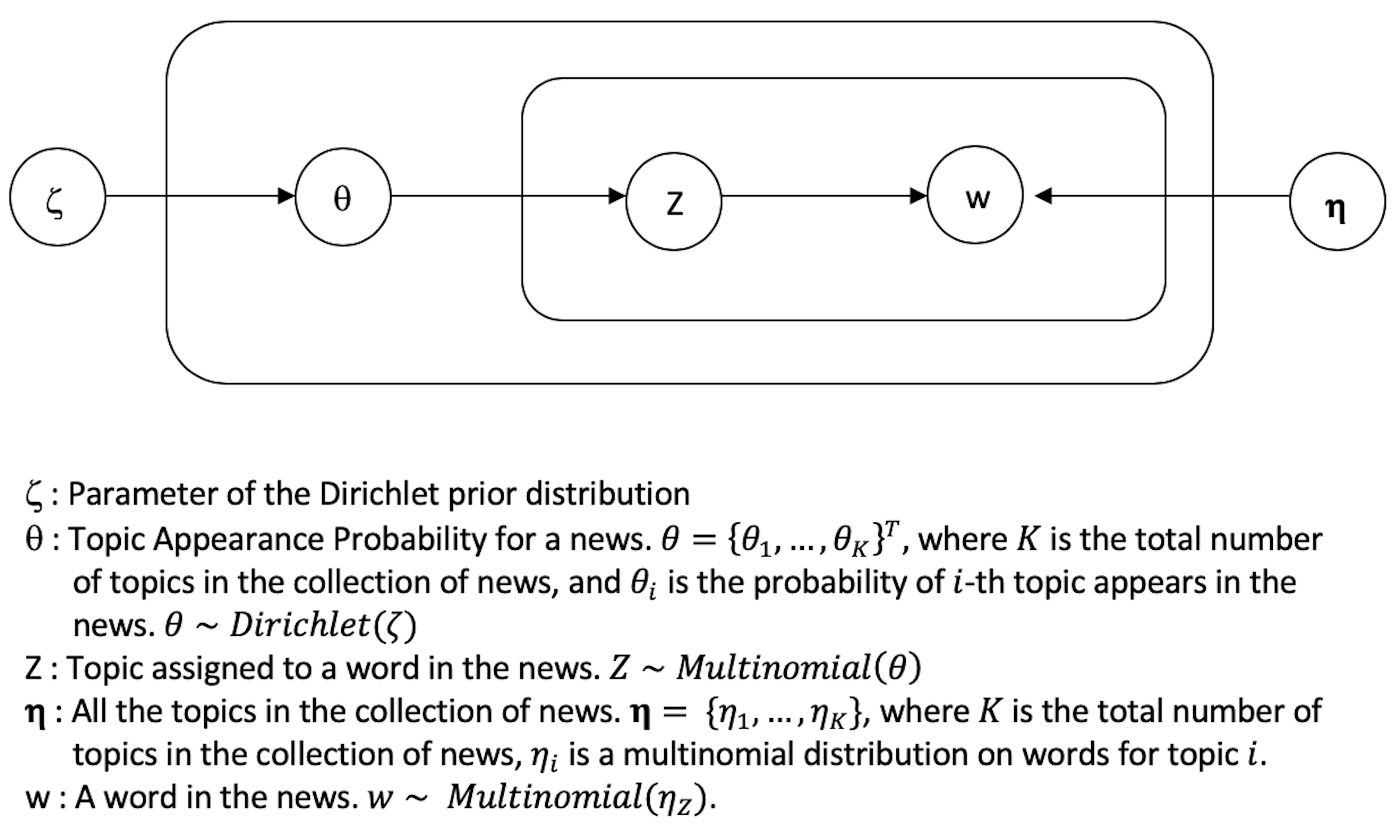
Figure 1: The graphical representation. The outer box represents the document level. The inner rectangle represents the word level.

The graphical representation is shown in Figure 1. The outer rectangle represents the document-level and the inner rectangle represents the word-level. $\zeta$ and $\eta$ are global parameters, i.e. shared by all the documents. $\theta$ and $Z$ are local latent variables. A complete Bayesian approach further assumes that topics $\eta_{1},\dots,\eta_{K}$ are generated from a Dirichlet prior with hyperparameter $\beta$. Here we use this formulation as in Blei et al. (2003) for the ease of adding a penalty.

The latent parameters in ETM are estimated by maximizing the following penalized posterior.

$$\max\hskip 5.69054ptp(\theta,Z,\zeta,\eta|W)-\sum_{i=1}^{K}\sum_{j=1}^{V}\mu_{i}m_{ij}|\eta_{ij}|+\sum_{i=1,l\neq i}^{K}\nu_{il}D_{KL}(\eta_{i}||\eta_{l})$$ (1)

where $p(\theta,Z,\zeta,\eta|W)$ is the posterior. The second term is the weighted lasso penalty, in which $\mu_{i}$ is the penalty weight for topic $i$, $m_{ij}$ represents the weight for word $j$ in topic $i$ and is known. The third term is the pairwise KL divergence penalty, in which $D_{KL}(\eta_{i}||\eta_{l})$ represents the KL divergence between topic $i$ and $l$ and $\nu_{il}$ is the corresponding penalty weight.

Unfortunately, the posterior is intractable to compute. Instead, a ‘variational EM algorithm’ is used to maximize the Evidence Lower Bound (ELBO) (Blei et al., 2003, 2017) $L(\zeta,\eta,\gamma,\phi)$,

$$L(\zeta,\eta,\gamma,\phi) =E_{q}[\ln p(\theta,Z,W|\zeta,\eta)]-E_{q}[\ln q(\theta,Z|\gamma,\phi)]$$

$$\leq\ln p(W|\zeta,\eta)$$

where $p(.)$ is the density function derived from LDA and $q(\theta,Z|\gamma,\phi)$ is the mean-field variational distribution

$$q(\theta,Z|\gamma,\phi)=q(\theta|\gamma)\prod_{n=1}^{N}q(Z_{n}|\phi_{n})$$

where $N$ is the number of words in a document, $q(\theta|\gamma)\sim Dirichlet(\gamma)$, and $q(Z_{n}|\phi_{n})\sim Multinomial(\phi_{n})$. $E_{q}$ represents the expectation under the variational distribution. The inequality is a result of applying Jensen inequality. The data $W$ provides more evidence to our prior belief. Hence the name ELBO.

Therefore, in the actual optimization, we maximize the following penalized ELBO.

$$\max\hskip 5.69054ptL(\zeta,\eta,\gamma,\phi)-\sum_{i=1}^{K}\sum_{j=1}^{V}\mu_{i}m_{ij}|\eta_{ij}|+\sum_{i=1,l\neq i}^{K}\nu_{il}D_{KL}(\eta_{i}||\eta_{l})$$ (2)

Equation 2 is maximized in an ‘EM’-like procedure. In the E-step, the ELBO is maximized w.r.t. the local variational parameter $\phi,\gamma$ for every document, conditional on the global latent parameter $\eta,\zeta$. Since the penalties don’t contain any local variational parameters, the updating equations will be the same as that of LDA.

$$\phi_{ni}\propto\eta_{iw_{n}}\exp{E_{q}[\log(\theta_{i})|\gamma]}$$ (3)

$$\gamma_{i}=\zeta_{i}+\sum_{n=1}^{N}\phi_{ni}$$

where

$$\exp{E_{q}[\log(\theta_{i})|\gamma]}=\Psi(\gamma_{i})-\Psi(\sum_{l=1}^{K}\gamma_{l})$$

and $\Psi$ is the digamma function, i.e. the logarithmic derivative of the gamma function.

Then conditional on all the local latent variables $\phi,\gamma$, the penalized ELBO is maximized w.r.t. the latent global parameter $\eta,\zeta$. The global parameter $\zeta$ can be estimated using Newton’s method. In practice, $\zeta$ is often assumed to be a symmetric Dirichlet parameter.

2.2 Only Weighted Lasso Penalty: $\nu=0$

In this section, we consider the case where we only have the weighted lasso penalty, i.e. $\nu=0$.

$$\max\hskip 5.69054ptL(\zeta,\eta,\gamma,\phi)-\sum_{i=1}^{K}\sum_{j=1}^{V}\mu_{i}m_{ij}|\eta_{ij}|$$ (4)

subject to

$$\sum_{j=1}^{V}\eta_{ij}=1,\forall i\in\{1,\dots,K\}$$

$$\eta_{ij}\geq 0,\forall i,j$$

$$\sum_{i=1}^{K}\theta_{di}=1,\forall d$$

where $K$ and $V$ represent the number of topics and vocabulary size respectively and $\mu_{i}\geq 0$ is the penalty weight for topic $i$ and is selected using cross-validation, $\eta_{ij}$ represents the probability of the $j$th word in the topic $i$, $m_{ij}$ is the weight for $\eta_{ij}$ and is known in advance, reflecting the prior information about the topic-word distribution. One possible candidate for the weight is the document frequency, i.e. $m_{ij}=df_{j},\forall i,j$, where $df_{j}$ is the number of documents containing the word $j$. The larger the document frequency for the word $j$, the larger the penalty. Consider an extreme case that word $j$ appears in every document of the corpus. Due to it co-occurs with every other word, LDA would assign a large probability to it in every topic. As a result, word $j$ contains little information to distinguish one topic from another. It’s barely useful in the dimension reduction process, i.e. from word space to topic space. With the document frequency penalty, it will be penalized the most and result in a low probability in the topic distributions.

We emphasize that the penalized model is not constrained to only solving the frequently words dominance issue. Any weight reflecting the prior information about the topic distribution can be used to achieve the practitioners’ goal. We give an illustration here and in the simulation study 3.2. Often practitioners found the field-important words are not assigned large probabilities in the estimated topics. (One possible reason is that they appear infrequently in the underlying corpus.) But these keywords contain important information about the field and are crucial to distinguish one topic from another. And practitioners might prefer they appear in the top-$T$ words for easy topic interpretation (In practice, $T$ is usually set as $10$ or $20$). In this situation, practitioners can utilize our proposed model by assigning negative weights to these keywords and zero weights to all the other words. Simulation case 3.2 is devoted to the situation.

To further understand the penalization, we rewrite the optimization problem 4 in the following equivalent form.

$$\max\hskip 5.69054ptL(\zeta,\eta,\gamma,\phi)$$

subject to

$$\sum_{j=1}^{V}m_{ij}|\eta_{ij}|\leq\nu_{i},\forall i\in\{1,\dots,K\}$$

$$\sum_{j=1}^{V}\eta_{ij}=1,\forall i\in\{1,\dots,K\}$$

$$\eta_{ij}\geq 0,\forall i,j$$

$$\sum_{i=1}^{K}\theta_{di}=1,\forall d$$

where $\nu_{i}>0$ is a hyperparameter and there is a one-to-one correspondence between $\mu_{i}$ and $\nu_{i}$. The penalty alters the feasible region. Figure 2 plots the feasible regions of the topics of LDA and the df-weighted LASSO penalized LDA for a simple case of having two words $w_{1}$ and $w_{2}$. The document frequencies are 2 and 1 for the word $w_{1}$ and $w_{2}$, respectively. The black solid line in the left subplot represents the feasible region of LDA. The feasible region of the ETM is plotted in the right subplot. The blue dashed line is the penalty induced constraint line $2\eta_{1}+\eta_{2}=1.5$. Due to the extra constraint, the feasible region is reduced to the upper-left black solid line. As a result, the feasible probability range $\eta_{1}$ is reduced to $(0,0.5)$. A smaller weight will be assigned to the relatively more frequently appearing word $w_{1}$ in the estimated topic.

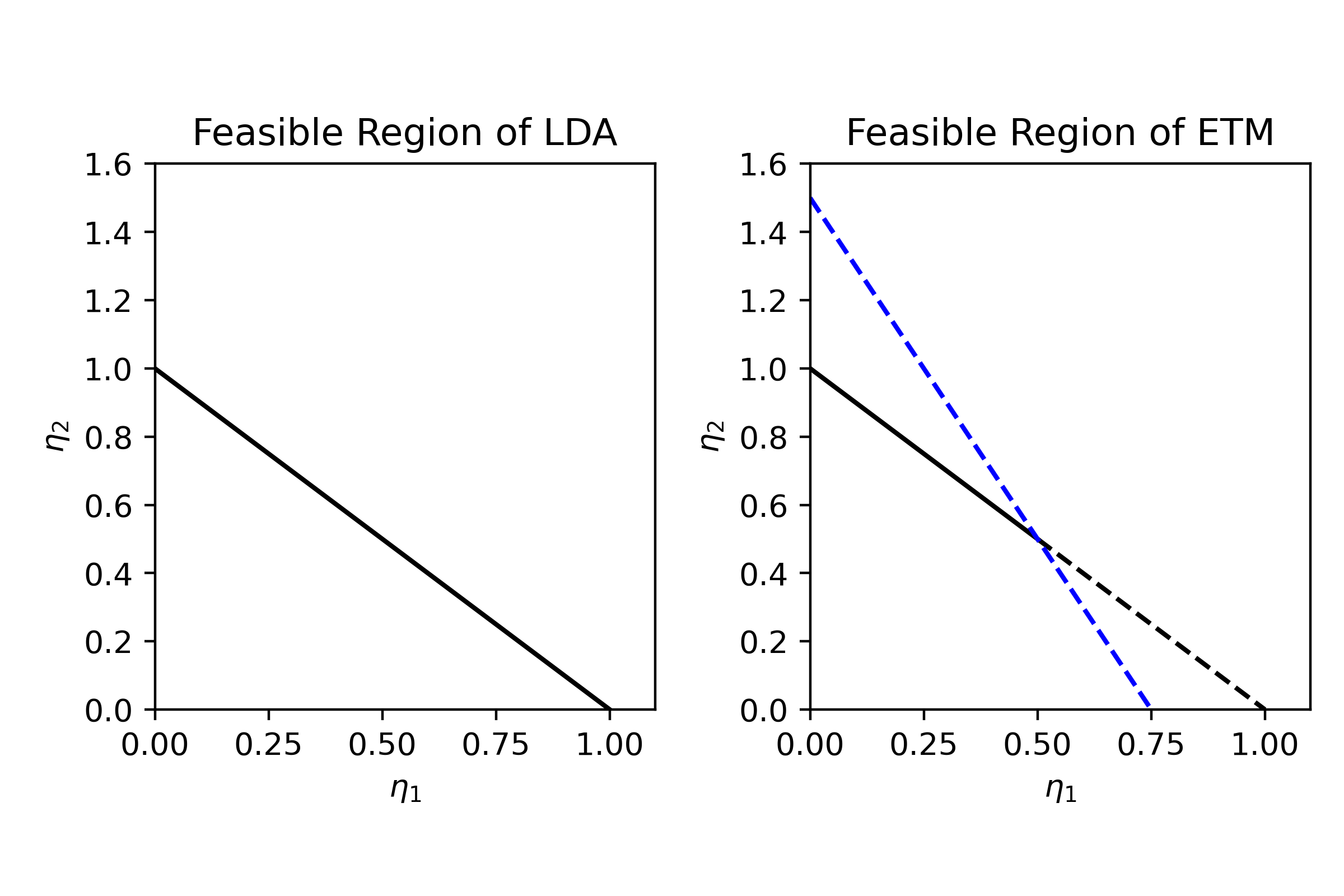
Figure 2: The feasible region of topics of LDA and ETM. The vocabulary consists of two words $w_{1}$ and $w_{2}$. Their corresponding document frequencies are 2 and 1, respectively. The feasible region of LDA topics is plotted in the left subplot as the solid black line. That of df-weighted LASSO penalized LDA is plotted in the right subplot. The blue dashed line is the penalty induced constraint line $2\eta_{1}+\eta_{2}=1.5$. The extra constraint reduces the feasible region of the topics to the top left black solid line. As a result, the feasible probability range $\eta_{1}$ is reduced to $(0,0.5)$. A smaller weight will be assigned to the relatively more frequently appearing word $w_{1}$ in the estimated topic.

As mentioned in section 2.1, the optimization is done using variational inference and the local latent parameters are updated the same as LDA, as given in equation 3. The global latent parameter $\eta$ is estimated by maximizing the following equation

$$\max\hskip 5.69054pt-f(\eta)=\sum_{d=1}^{D}\sum_{n=1}^{N_{d}}\sum_{i=1}^{K}\sum_{j=1}^{V}\phi_{dni}w_{dn}^{j}\log(\eta_{ij})-\sum_{i=1}^{K}\sum_{j=1}^{V}\mu_{i}m_{ij}|\eta_{ij}|$$

subject to

$$\sum_{j=1}^{V}\eta_{ij}=1,\forall i\in\{1,\dots,K\}$$

$$\eta_{ij}\geq 0,\forall i,j$$

where the first term is by taking out all the terms containing $\eta$ from ELBO. The problem can be further reduced to $K$ sub-optimization problems below. Due to $\log(\eta_{ij})$ in the target function, the constraint $\eta_{ij}\geq 0,\forall i,j$ can be ignored. The absolute value $|\eta_{ij}|$ in the target function equals $\eta_{ij}$. We rewrite the maximization as an equivalent minimization problem.

$$\min\hskip 5.69054ptf_{i}(\eta_{i})=-\sum_{d=1}^{D}\sum_{n=1}^{N_{d}}\sum_{j=1}^{V}\phi_{dni}w_{dn}^{j}\log(\eta_{ij})+\sum_{j=1}^{V}\mu_{i}m_{ij}\eta_{ij}$$ (5)

subject to

$$\sum_{j=1}^{V}\eta_{ij}=1$$

We use the Newton method with equality constraints (Boyd et al., 2004) to solve equation 5. The updating direction $\Delta\eta_{i}$ with a feasible starting point $\eta_{i}^{0}$ can be calculated using the following equation

$$\begin{bmatrix}\nabla^{2}f_{i}&\mathbf{1}\\ \mathbf{1}^{T}&0\par\end{bmatrix}\begin{pmatrix}\Delta\eta_{i}\\ \alpha_{i}\end{pmatrix}=\begin{pmatrix}-\nabla f_{i}\\ 0\end{pmatrix}$$

The updating direction is

$$\Delta\eta_{ij}=\frac{-f^{\prime}_{ij}-\alpha_{i}}{f^{\prime\prime}_{ij}}=\eta_{ij}-\frac{(\alpha_{i}+\mu_{i}m_{ij})\eta_{ij}^{2}}{\sum_{d=1}^{D}\sum_{n=1}^{N_{d}}\phi_{dni}w_{dn}^{j}}$$ (6)

where $f^{\prime}_{ij}$ and $f^{\prime\prime}_{ij}$ are the first and second partial derivatives of $f_{i}$ with respect to $\eta_{j}$, and

$$\alpha_{i}=\frac{-\sum_{j=1}^{V}f^{\prime}_{ij}/f^{\prime\prime}_{ij}}{\sum_{j=1}^{V}1/f^{\prime\prime}_{ij}}=\frac{\sum_{j=1}^{V}\left(\eta_{ij}-\frac{\mu_{i}m_{ij}\eta_{ij}^{2}}{\sum_{d=1}^{D}\sum_{n=1}^{N_{d}}\phi_{dni}w_{dn}^{j}}\right)}{\sum_{j=1}^{V}\frac{\eta_{ij}^{2}}{\sum_{d=1}^{D}\sum_{n=1}^{N_{d}}\phi_{dni}w_{dn}^{j}}}$$

The Newton decrement is

$$\lambda(\eta_{i})=(\Delta\eta_{i}^{T}\nabla^{2}f_{i}\Delta\eta_{i})^{1/2}=\left(\sum_{j=1}^{V}\frac{(\sum_{d=1}^{D}\sum_{n=1}^{N_{d}}\phi_{dni}w_{dn}^{j}-(\alpha_{i}+\mu_{i}m_{ij})\eta_{ij})^{2}}{\sum_{d=1}^{D}\sum_{n=1}^{N_{d}}\phi_{dni}w_{dn}^{j}}\right)^{1/2}$$ (7)

We use the backtracking line search (Boyd et al., 2004) to estimate the step size. The complete step to estimate topics of the weighted LASSO penalized LDA is given in algorithm 1.

Result: Update the $i$th topic word distribution $\eta_{i}$

Initialize $\eta_{i}$ with a feasible point;

Choose the stopping criteria $\epsilon$ and the line search parameter $\delta\in(0,0.5)$, $\gamma\in(0,1)$;

while not reaching the maximum iteration do

       Compute the feasible descent direction $\Delta\eta_{i}$ and Newton decrement $\lambda(\eta_{i})$ ;

       if $\lambda(\eta_{i})^{2}/2\leq\epsilon$ then

             Stop the algorithm ;

      else

            Find step size $t$ by backtracking line search:
Initialize the step size $t\coloneqq 1$ ;

             while $f_{i}(\eta_{i}+t\Delta\eta_{i})>f_{i}(\eta_{i})+\delta t\nabla f_{i}^{T}\Delta\eta$ do

                   $t\coloneqq\gamma t$;

             end while

            

       end if

      $\eta_{i}\coloneqq\eta_{i}+t\Delta\eta_{i}$;

end while

Algorithm 1 Variational m-step

2.3 Only Pairwise Kullback-Leibler Divergence Penalty: $\mu=0$

Practitioners often find some estimated topics are ’close’ to each other, in the sense, they have similar semantic meaning and share several common words in their top-$N$ words. It makes the topic interpretation and the analyzing steps following topic modeling, e.g. Lei et al. (2020), difficult. In this section, we consider the case where we only have a pairwise KL divergence penalty, i.e. $\mu=0$. The optimization takes the following form.

$$\max\hskip 5.69054ptL(\zeta,\eta,\gamma,\phi)+\sum_{i=1,l\neq i}^{K}\mu_{il}D_{KL}(\eta_{i}||\eta_{l})$$ (8)

subject to

$$\sum_{j=1}^{V}\eta_{ij}=1,\forall i\in\{1,\dots,K\}$$

$$\eta_{ij}\geq 0,\forall i,j$$

$$\sum_{i=1}^{K}\theta_{di}=1,\forall d$$

where $D_{KL}(\eta_{i}||\eta_{l})$ is the KL divergence between topic $i$ and $l$

$$D_{KL}(\eta_{i}||\eta_{l})=\sum_{j=1}^{V}\eta_{ij}\log(\frac{\eta_{ij}}{\eta_{lj}})$$

Since the penalty only involves topic distribution $\eta$ and thus only plays a role in the M-step. The E-step is the same as equation 3. For the M-step, we optimize

$$\min\hskip 5.69054ptg(\eta)=-\sum_{d=1}^{D}\sum_{n=1}^{N_{d}}\sum_{i=1}^{K}\sum_{j=1}^{V}\phi_{dni}w_{dn}^{j}\log(\eta_{ij})-\sum_{i=1,l\neq i}^{K}\sum_{j=1}^{V}\mu_{il}\eta_{ij}\log(\frac{\eta_{ij}}{\eta_{lj}})$$ (9)

subject to

$$\sum_{j=1}^{V}\eta_{ij}=1,\forall i\in\{1,\dots,K\}$$

$$\eta_{ij}\geq 0,\forall i,j$$

There are two differences between the current optimization and the optimization in section 2.2 : 1) the optimization can no longer be separated into $K$ sub-optimization problems as the different topics are now intertwined through the penalty; 2)the objective function is no long convex. For the first difference, we borrow the idea of coordinate descent and sequentially optimize one topic at a time while conditioning on all the other topics. The benefit of this approach instead of updating all topics simultaneously is that it simplifies the constrained Newton updating equation involving the Hessian matrix. Under the conditional approach, the Hessian matrix for a particular topic $\nabla^{2}g_{i}$ is diagonal. For the second difference, due to the non-convexity, the Hessian matrix may not be positive semi-definite. As a result, Newton decrement could be a complex number. We use a combination of gradient descent and Hessian descent algorithm to tackle the second issue (Nesterov and Polyak, 2006, Allen-Zhu and Li, 2018). The Hessian descent is invoked when the Hessian is not positive semi-definite. The Hessian descent moves to a smaller value along the Newton direction.

We now show the updating equations for the gradient descent step. For topic $i$ while conditioning on all the other topics, we optimize the following equation

$$\min\hskip 5.69054ptg_{i}(\eta_{i}|\eta_{l},l\neq i)=-\sum_{d=1}^{D}\sum_{n=1}^{N_{d}}\sum_{j=1}^{V}\phi_{dni}w_{dn}^{j}\log(\eta_{ij})-\sum_{l\neq i}\sum_{j=1}^{V}\mu_{il}\eta_{ij}\log(\frac{\eta_{ij}}{\eta_{lj}})-\sum_{l\neq i}\sum_{j=1}^{V}\mu_{li}\eta_{lj}\log(\frac{\eta_{lj}}{\eta_{ij}})$$ (10)

subject to

$$\sum_{j=1}^{V}\eta_{ij}=1$$ (11)

The updating direction $\Delta\eta_{i}$ with a feasible starting point $\eta_{i}^{0}$ can be calculated using the following equation

$$\begin{bmatrix}\nabla^{2}g_{i}&\mathbf{1}\\ \mathbf{1}^{T}&0\par\end{bmatrix}\begin{pmatrix}\Delta\eta_{i}\\ \alpha_{i}\end{pmatrix}=\begin{pmatrix}-\nabla g_{i}\\ 0\end{pmatrix}$$ (12)

The updating direction is

$$\Delta\eta_{ij}=\frac{-g^{\prime}_{ij}-\alpha_{i}}{g^{\prime\prime}_{ij}}=\frac{\eta_{ij}(\sum_{d=1}^{D}\sum_{n=1}^{N_{d}}\phi_{dni}w_{dn}^{j}-\sum_{l\neq i}\mu_{li}\eta_{lj})+\eta_{ij}^{2}\big{(}\sum_{l\neq i}\mu_{il}(\log\eta_{ij}-\log\eta_{lj}+1)-\alpha_{i}\big{)}}{\sum_{d=1}^{D}\sum_{n=1}^{N_{d}}\phi_{dni}w_{dn}^{j}-\sum_{l\neq i}\mu_{li}\eta_{lj}-\eta_{ij}\sum_{l\neq i}\mu_{il}}$$ (13)

where $g^{\prime}_{ij}$ and $g^{\prime\prime}_{ij}$ are the first and second partial derivatives of $g_{i}$ with respect to $\eta_{j}$, and

$$\alpha_{i}=\frac{-\sum_{j=1}^{V}g^{\prime}_{ij}/g^{\prime\prime}_{ij}}{\sum_{j=1}^{V}1/g^{\prime\prime}_{ij}}=\frac{\sum_{j=1}^{V}\frac{\eta_{ij}(\sum_{d=1}^{D}\sum_{n=1}^{N_{d}}\phi_{dni}w_{dn}^{j}-\sum_{l\neq i}\mu_{li}\eta_{lj})+\eta_{ij}^{2}\big{(}\sum_{l\neq i}\mu_{il}(\log\eta_{ij}-\log\eta_{lj}+1)\big{)}}{\sum_{d=1}^{D}\sum_{n=1}^{N_{d}}\phi_{dni}w_{dn}^{j}-\sum_{l\neq i}\mu_{li}\eta_{lj}-\eta_{ij}\sum_{l\neq i}\mu_{il}}}{\sum_{j=1}^{V}\frac{\eta_{ij}^{2}}{\sum_{d=1}^{D}\sum_{n=1}^{N_{d}}\phi_{dni}w_{dn}^{j}-\sum_{l\neq i}\mu_{li}\eta_{lj}-\eta_{ij}\sum_{l\neq i}\mu_{il}}}$$ (14)

The Newton decrement is

$$\lambda(\eta_{i}) =(\Delta\eta_{i}^{T}\nabla^{2}g_{i}\Delta\eta_{i})^{1/2}$$

$$=\left(\sum_{j=1}^{V}\frac{\Big{(}\sum_{d=1}^{D}\sum_{n=1}^{N_{d}}\phi_{dni}w_{dn}^{j}-\sum_{l\neq i}\mu_{li}\eta_{lj}+\eta_{ij}\big{(}\sum_{l\neq i}\mu_{il}(\log\eta_{ij}-\log\eta_{lj}+1)-\alpha_{i}\big{)}\Big{)}^{2}}{\sum_{d=1}^{D}\sum_{n=1}^{N_{d}}\phi_{dni}w_{dn}^{j}-\sum_{l\neq i}\mu_{li}\eta_{lj}-\eta_{ij}\sum_{l\neq i}\mu_{il}}\right)^{1/2}$$

Due to the non-convexity, $\Delta\eta_{i}^{T}\nabla^{2}g_{i}\Delta\eta_{i}$ could be negative at some points. When it happens, the Hessian descent is invoked and finds a new position along $\Delta\eta_{i}$ with smaller values (see details in Algorithm 2).

To update all the topics, we optimize the topics sequentially and stops until an overall convergence measured by the Frobenius norm of the successive updates, as in Algorithm 2.

Result: Update the topic word distribution $\eta$

Initialize the topic word distribution $\eta^{0}$ with a feasible point for every topic $\eta^{0}_{i},i=1,\dots,K$;

Choose the stopping criterion $\epsilon$;

while $||\eta^{t+1}-\eta^{t}||_{F}>\epsilon$ do

       for topic $i,i=1,\dots,K$ do

             if $\Delta\eta_{i}^{T}\nabla^{2}f_{i}\Delta\eta_{i}\geq 0$ then

                   Gradient Descent:
update topic word distribution $\eta_{i}|\eta_{j},j\neq i$ using algorithm 1

            else

                  Hessian Descent:
find step size $h$ satisfying $\eta_{i}+h\Delta\eta_{i}>0$ and $\eta_{i}-h\Delta\eta_{i}>0$;

                   if $g_{i}(\eta_{i}+h\Delta\eta_{i})>g_{i}(\eta_{i}-h\Delta\eta_{i})$ then

                        $\eta_{i}\coloneqq\eta_{i}-h\Delta\eta_{i}$

                  else

                        $\eta_{i}\coloneqq\eta_{i}+h\Delta\eta_{i}$

                   end if

                  

             end if

            

       end for

      

end while

Algorithm 2 Variational m-step for the pairwise KL-Divergence

2.4 Dynamic penalty weight implementation and the combination of two penalties

Both Algorithm 1 and 2 apply to the variational m-step. Recall that the ELBO is maximized by an iterative variational EM algorithm. The m-step depends on the e-step output, i.e. $\phi_{dni}w_{dn}^{j}$ in equation 5 and 10. In each iteration, E-step would possibly produce $\phi_{dni}w_{dn}^{j}$ of different scales, especially at the beginning of the iterations. A penalty weight appropriate for the current iteration may be too big(small) for the next iteration. Therefore we reparameterize the penalty weight $\mu_{i}$ as $\nu_{i}*\max_{j}(\sum_{dn}\phi_{dni}w_{dn}^{j})$ in the final variational EM algorithm. The reparameterization makes the penalty similar scale as its ELBO part, and thus effective in every EM iteration.

The combination of two penalties in a single algorithm is straightforward. Algorithm 2 can be used for the combined penalties. Adding the weighted lasso penalty changes the updating direction $\Delta\eta$ and the Newton decrement $\lambda(\eta)$ in the gradient descent, as it alters the first derivative by subtracting the weights.

3 Simulation

In this section, we use simulated data to demonstrate the effectiveness of the proposed ETM. In section 3.1, we simulate the situation that the corpus contains several frequently appearing words. Comparing to LDA, ETM effectively avoids the frequent word dominance issue in the estimated topics. In section 3.2, we simulate the case in which field-important words appear infrequently in the underlying corpus. ETM is able to reveal the importance of these words and recover the true distribution using negative weights on these words and zero weights on all the other words, while LDA is not. In section 3.3, we simulate a ’close’ estimated topic situation, by adding several frequently appearing words. LDA topics share these frequently appearing words in their corresponding top-$T$ words. If practitioners interpret topics based on these top-$T$ words, they might mistakenly interpret them as the same topic. ETM is able to separate the topics and at the same time recovers the true topics.

3.1 Case 1: Corpus-specific common words

The setup is as follows. The number of topics $K$ is 2. The prior $\zeta=0.1$. Topic word distribution $\eta$ is randomly drawn from a Dirichlet prior $\eta\sim Dir(0.1*\mathbbm{1})$ where $\mathbbm{1}$ is a $300\times 1$ vector of $1$s. Then we use the word generating process of LDA to generate the words for a corpus containing $500$ documents. During the word generation, we set an upper limit on the maximum number of words in every document to be $100$. Some words don’t appear in the corpus due to small topic word probabilities assigned to them. Thus the number of generated words is 202. We further assume that the corpus contains 3 corpus-specific common words 301, 302, 303 and each of them randomly appears in $50\%$ of the documents. The appearance frequency in a document is 3. These words are then added to the generated corpus. In total, we have $205$ words (202 generated words + 3 manually inserted words) in our final corpus.

We apply the LDA and ETM ($\nu=0$) to the simulated corpus. The weights are the document frequencies of all words scaled to a maximum of 100. The penalty weight is selected to be $\mu=0.3$. In practice, the estimated topics are interpreted using their corresponding top-$T$ words. We list the top 10 words of true topics, LDA estimated topics, and ETM topics in Table 1. The corpus-specific common words 301, 302, 303 are assigned high probabilities in LDA and appear in the top 10 words. The probabilities of these 3 words in ETM are about half of those in LDA (a further reduction is achievable with a larger penalty). The high probabilities assigned to these frequently appearing words not only make the topic interpretation difficult, but also distort the document topic frequencies $\theta$, and thus reduce the accuracy of information retrieval.

Topic 1	Top 10 words
True	47	83	86	81	153	270	80	14	291	258
LDA	47	303	302	301	83	86	81	270	153	80
ETM	47	86	83	153	81	14	258	30	270	196
Topic 2	Top 10 words
True	170	256	206	0	219	286	243	114	132	82
LDA	170	206	256	0	301	303	302	219	243	114
ETM	170	206	256	219	243	114	0	286	82	132

Table 1: Top 10 words of the true topics, LDA estimated topics and ETM estimated topics of the simulation study. The corpus-specific frequently appearing words 301, 302, 303 appear in the LDA estimated topics, but not in the ETM estimated topics. The large probabilities assigned to these frequently appearing words 301, 302, 303 not only make the topic interpretation difficult but also distort the document topic distribution $\theta$, which reduces the accuracy of information retrieval. The weights are the document frequencies of all words scaled to a maximum of 100. The penalty weight is selected to be 0.3.

We repeat the above procedure 1000 times and record the number of corpus-specific common words appearing in the top 10 words and the ratio of the average probabilities of these three words in ETM and those in LDA. The summary statistics are given in Table 2. Row 1 is the summary statistics for the number of common words appearing in the top 10 words of LDA topics. The minimum and maximum are 4 and 6, respectively. The mean is 5.989 and the variance is 0.013. It indicates that these 3 corpus-specific common words almost always appear in the top 10 words of LDA estimated topics. Row 2 lists the summary statistics of the number of common words appearing in the top 10 words of document frequency ETM. Its minimum and maximum are 0 and 6, respectively. The mean is 0.585 and the variance is 1.410. It indicates that the majority of the simulation gets no common words in the top 10 words of the ETM estimated topics. The last row shows the summary statistics of the ratio of average probabilities of these three corpus-specific common words in ETM and those in LDA. The minimum and maximum are 0.113 and 0.547. The mean is 0.322 and the variance is 0.004. It indicates that on average, the probabilities assigned to these corpus-specific common words in the ETM are about 1/3 of those in LDA.

	min	max	mean	variance
LDA: number of common words	4	6	5.989	0.013
ETM: number of common words	0	6	0.585	1.410
Ratio of common words average probabilities	0.113	0.547	0.322	0.004

Table 2: Summary statistics of 1000 repetition. The first row reports the statistics of the number of common words appearing in the top 10 words of LDA topics. The average is 5.989 and the variance is 0.013, which indicates that these three common words almost always appear in every LDA topic. The second row reports the statistics of the number of common words appearing in the top 10 of ETM topics. The average is 0.585 and the variance is 1.410, indicating the majority don’t have the common words in their top 10. The last row lists the statistics of the ratio of the average probabilities of these three common words in ETM and that in LDA. The mean is 0.322 and the variance is 0.004, indicating that on average the probabilities assigned to these three common words in ETM are about 1/3 of those in LDA.

3.2 Case 2: Important words appear rarely in the corpus

We consider another situation. In practice, certain words are important for that field. But unfortunately, they appear rarely in the current corpus. Practitioners might perceive these words as very important and would like them to be assigned high probability in the topic word distribution. The LDA word generating process is the same as before. Namely, the corpus contains 2 topics. The prior $\zeta=0.1$. Topic word distribution $\eta$ is randomly drawn from a Dirichlet prior $\eta\sim Dir(0.1*\mathbbm{1})$ where $\mathbbm{1}$ is a $300\times 1$ vector of $1$s. We assume that due to some reason, the top 2 words in each topic appear rarely in the current corpus. They only appear in $10\%$ of the total documents, i.e. we randomly select 50 documents containing the top words and delete them from the remaining documents containing them.

We then apply LDA and ETM ($\nu=0$) to these words. Different from the previous setup in which corpus-specific common words are not known and we use document frequencies as weights, these important words are known and we assign negative weights to them and zero weights to all the other words. In the simulation, words 275 and 22 are important for topic 1, and words 73, 195 are important for topic 2. Their total appearance is limited to 50 documents, i.e. $10\%$ of the corpus size. Due to their rare appearance, LDA is unable to recover their importance and small probabilities are assigned to them. They don’t appear in the top 10 words of LDA topics. By assigning weight -100 to these four words and penalty weight $\mu=0.2$, ETM successfully recovers their position in the top 10 words of the estimated topics.

Topic 1	Top 10 words
True	275	22	110	251	291	151	171	18	253	187
LDA	110	251	151	291	171	253	18	187	35	287
ETM	275	22	110	251	151	291	171	253	18	187
Topic 2	Top 10 words
True	73	195	294	207	48	248	19	211	43	175
LDA	294	207	48	248	19	43	211	175	269	213
ETM	73	195	294	207	48	248	19	43	211	175

Table 3: Top 10 words of the true topics, LDA estimated topics and ETM estimated topics of the simulation study. We assume that words 275, 22, 73, 195 are important words of the field, but appears rarely in the current corpus. Because of their rare appearance, LDA is unable to recover them and restore their importance in the topic word distribution. ETM is able to capture the importance of these words, by assigning negative weights to them and zero weights to all the other words. The field important words are usually known in advance by practitioners. Here we assign weights -100 to words 275, 22, 73, 195, and 0 to all the other words. The penalty ratio is 0.2.

We repeat the above procedure 1000 times. The summary statistics are reported in Table 4. Row 1 reports the number of important words appearing in the top 10 of LDA estimated topics. The minimum and maximum are 0 and 3, respectively. The mean is 0.299 and the variance is 0.288. It indicates that these important but rarely appearing words barely appear in the top 10 words of LDA topics, i.e. LDA is unable to restore their importance. Row 2 reports the number of important but infrequent words appearing in the top 10 of ETM topics. The minimum and maximum are 2 and 4, respectively. The mean is 3.993 and the variance is 0.009. It indicates that these words are almost always recovered by the ETM. The last row reports the statistics of the average ratio between the probabilities assigned to these important but rarely appearing words in the ETM and those in the LDA. The minimum and maximum are 4.187 and 24.857, respectively. The average is 9.767 and the variance is 6.427. It indicates that on average the probabilities assigned to these important but rarely appearing words are about 10 times in the ETM than those in LDA.

	min	max	mean	variance
LDA: number of rare important words	0	3	0.299	0.288
LASSO LDA: number of rare important words	2	4	3.993	0.009
Ratio of rare important words average probabilities	4.187	24.853	9.767	6.427

Table 4: Summary statistics of 1000 repetition. The first row reports the statistics of the number of rarely appearing but important words appearing in the top 10 words of LDA topics. The average is 0.299 and the variance is 0.288, which indicates that these important but rarely appearing words seldom appear in the top 10 words of LDA estimated topics. The second row reports the statistics of the number of important but rarely appearing words appearing in the top 10 of ETM topics. The average is 3.993 and the variance is 0.009, indicating the ETM successfully recovers the important words. The last row lists the statistics of the ratio of the average probabilities of these important but rarely appearing words in ETM and that in LDA. The mean is 9.767 and the variance is 6.427, indicating that on average the probabilities assigned to these words in ETM are about 10 times of those in LDA.

3.3 Case 3: ‘Close’ topics

Practitioners often find some estimated topics are ’close’ to each other. By ’close’, we mean the estimated topics share several common words and have similar semantic meaning. The exact reason for this phenomenon is unclear. We hypothesize that it is due to the exchangeability assumption of words in LDA. Nevertheless, we simulate the case using frequently appearing words. The basic set up is similar to Case 1. Namely, the corpus contains 2 topics. The prior $\zeta=0.1$. Topic word distribution $\eta$ is randomly drawn from a Dirichlet prior $\eta\sim Dir(0.1*\mathbbm{1})$ where $\mathbbm{1}$ is a $300\times 1$ vector of $1$s. To simulate the estimated ’close’ topics in LDA, we further add 6 common words 301, 302, 303, 304, 305, 306 to the corpus and assume that they appear in $80\%$ of the documents. With this setup, we apply LDA and ETM ($\mu=0$) with penalty weight for the pairwise KL divergence $\nu=0.5$ to the simulated corpus. The true and estimated topics are listed in Table 5. Because of the dominance of frequently appearing words, the LDA topics are ’close’ to each other, as by our design. The ETM clearly separates them. Although the appearing sequence of ETM is slightly different from the true model, the number of same words appearing in both true and ETM are 8 for both topic 1 and 2, while that for true topics and LDA are 4 and 5 for topic 1 and 2 respectively. The Jensen-Shannon divergence of the true, LDA, and ETM topics are $0.81,0.63,0.88$, respectively.

Topic 1	Top 10 words
True	196	56	166	122	219	161	18	104	276	86
LDA	196	56	166	122	301	303	306	302	305	304
ETM	134	56	196	122	161	166	86	219	104	301
Topic 2	Top 10 words
True	46	165	115	140	53	280	138	19	174	290
LDA	46	165	115	304	140	305	302	306	280	303
ETM	85	46	165	140	115	280	53	19	304	138

Table 5: Top 10 words of the true topics, LDA estimated topics and ETM estimated topics of the simulation study. Due to the frequently appearing words, LDA topics are ’close’ to each other. Although the ETM produce the wrong word sequence, they share 8 words with the true topics for both topic 1 and 2, while LDA only has 4 and 5 shared words for topic 1 and 2. Moreover, the Jensen-Shannon divergence of the true topics, topics estimated by LDA, and topics estimated by ETM are $0.81,0.63,0.88$, respectively.

We repeat the simulation 1,000 times and report the summary statistics in Table 6. The first column shows the number of shared top 10 words between topics 0 and topic 1. The true topics on average share $0.34$ words with a standard deviation of $0.57$. LDA estimated topics on average share $3.10$ words with a standard deviation of $1.61$. ETM on average share $0.08$ words with a standard deviation of $0.30$. It shows the ETM is capable of separating the ’close’ topics and making them share few words in their top words. While the first column focus on the top words, the second column is on the overall topic distribution. It reports the Jensen-Shannon Divergence(JSD) of the topic distributions. The JSD of the true topic is on average $0.80$ with a standard deviation of $0.05$, while LDA is on average $0.64$ with a standard deviation of $0.04$, and ETM is on average $0.79$ with a standard deviation of $0.06$. It shows the ETM separates the ’close’ topics. The last two columns report the number of shared top 10 words between the true topics and estimated topics. It doesn’t make sense if the ETM separates topics but makes the estimation far away from the true topics. Because of the setup, LDA topic and the true topics on average share $5.54$ and $5.50$ words with standard deviations being $1.24$ and $1.19$ for topics 0 and 1, respectively. ETM and the true topics share on average $8.23$ and $8.20$ words with standard deviation being $1.25$ and $1.28$, respectively. It means that judging from the top-$T$ words, the ETM topics are semantically close to the true model.

	# of shared top 10 words between topics 0 and 1	JSD	# of shared top 10 words between true topic 0 and estimated topic 0	# of shared top 10 words between true topic 1 and estimated topic 1
True	0.34	0.80
	(0.57)	(0.05)
LDA	3.10	0.64	5.54	5.50
	(1.61)	(0.04)	(1.24)	(1.19)
KL Div	0.08	0.79	8.23	8.20
	(0.30)	(0.06)	(1.25)	(1.28)

Table 6: Summary statistics of 1000 repetition. The first column shows the mean and standard deviation of the number of shared top 10 words between topics 0 and 1.The values show that ETM is capable of separating the ’close’ topics and their top words share few common words. The second column reports the mean and standard deviation of the corresponding Jensen-Shannon Divergence. On average, the ETM topics are separated and their average JSD is similar to the true topics. The last two columns report the number of shared words between the true topic and the estimated topic. ETM on average shares about $8.2$ words with the true model, meaning the ETM topics are close to the true topics.

4 Real Data Application

To test the empirical performance of our proposed method, we apply LDA, ETM with lasso penalty only($\nu=0$), and ETM with pairwise KL divergence only ($\mu=0$) to the NIPS dataset, which consists of 11,463 words and 7,241 NIPS conference paper from 1987 to 2017. The data is randomly split into two parts: training (80%) and testing (20%). We select the number of topics for LDA using cross-validation with perplexity on the training dataset (Blei et al., 2003). The selected number is assumed to be the true number of topics in the NIPS dataset. The candidates are $\{5,10,15,20,25,30\}$. $K=10$ produces the lowest average validation perplexity. For ETM, we use homogeneous hyperparameters in this experiment, i.e. $\mu_{i}=\mu,\forall i\in\{1,\dots,K\}$ for the weighted lasso penalty and $\nu_{il}=\nu,\forall i,l\in\{1,\dots,K\}\text{ and }l\neq i$ for the pairwise KL divergence penalty, as we don’t have any prior information on the topics.

We do cross-validation on the training data to select the penalty weight $\mu$. When selecting $\mu$, perplexity is no longer an appropriate measure. Perplexity is the negative likelihood per word. A higher probability of frequently appearing words will produce a lower perplexity. As a result, $\mu=0$ will be selected. Another commonly used metric to select hyperparameters is the topic coherence score. Researchers have proposed several calculation methods of the topic coherence scores (Newman et al., 2010, Mimno et al., 2011, Aletras and Stevenson, 2013, Röder et al., 2015). Röder et al. (2015) show that among all these proposed topic coherence scores, $C_{V}$ achieves the highest correlation with all available human topic ranking data (also see Syed and Spruit (2017)). Roughly speaking, $C_{V}$ takes into consideration both generalization and localization of the topics. Generalization means $C_{V}$ measures the performance on the unseeable test dataset. Localization means $C_{V}$ uses a rolling window to measure the word’s co-occurrence.

In this paragraph, we provide the details of $C_{V}$ calculation. The top $N$ words of each topic are selected as the representation of the topic, denoted as $W=\{w_{1},\dots,w_{N}\}$. Each word $w_{i}$ is represented by an $N$-dimensional vector $v(w_{i})=\{NPMI(w_{i},w_{j})\}_{j=1,\dots,N}$, where $j$th-entry is the Normalized Pointwise Mutual Information(NPMI) between word $w_{i}$ and $w_{j}$, i.e. $NPMI(w_{i},w_{j})=\frac{\log P(w_{i},w_{j})-\log(P(w_{i})P(w_{j}))}{-\log P(w_{i},w_{j})}$. $W$ is represented by the sum of all word vectors, $v(W)=\sum_{j=1}^{N}v(w_{j})$. The calculation of NPMI between word $w_{i}$ and $w_{j}$ involves the marginal and joint probabilities $p(w_{i}),p(w_{j}),p(w_{i},w_{j})$. A sliding window of size 110, which is the default value in the python package ’gensim’ and robust for many applications, is used to create pseudo-document and estimate the probabilities. The purpose of the sliding window is to take the distance between two words into consideration. For each word $w_{i}$, a pair is formed $(v(w_{i}),v(W))$. A cosine similarity measure $\phi_{i}(v(w_{i}),v(W))=\frac{v(w_{i})^{T}v(W)}{\left\lVert v(w_{i})\right\rVert\left\lVert v(W)\right\rVert}$ is then calculated for each pair. The final $C_{V}$ score for the topic is the average of all $\phi_{i}$s.

We use $C_{V}$ to select the penalty weight from $\{0,0.5,1,1.5,2,2.5,3\}$. $\mu=0.5$ produces the highest average coherence score 0.56 for ETM, while $\mu=0$, i.e. LDA, gives the coherence score 0.51. We then refit both LDA and ETM ($\mu=0.5,\nu=0$) to the whole training dataset and use the test dataset to calculate the coherence score $C_{V}$ as a final evaluation of the performance on unseeable data. The results are shown in Table 4. Overall the $C_{V}$ score of LDA topics is 0.51 and that of ETM is 0.62, a $22\%$ improvement. We highlight two common words ’data’ and ’using’ in the top 20 words of both topics. They appear more frequently in LDA topics than in ETM topics. Both words appear in 5 out of 10 LDA topics and 1 out of 10 ETM topics. We also observe some large improvements for topic Reinforcement Learning, Neural Network, Computer Vision, and several other topics. Take Reinforcement Learning as an example. Comparing the top 20 words, we observe that words time, value, function, model, based, problem appear in LDA topic, but not the ETM topic. Surely these words are associated with reinforcement learning, but they are also associated with topics Neural Network, Bayesian, Optimization, etc. We refer these words as corpus-specific common words, i.e. for the current corpus, they contain little information to distinguish one topic from another. Their positions in the ETM topic are filled by words game, trajectory, robot, control. These words are related to the applications of reinforcement learning and represent the topics better than the previous corpus-specific common words. We see the $C_{V}$ score increased from 0.56 to 0.77, a $38\%$ increase. We do observe that an LDA topic related to NLP is missing in ETM. One possible reason is that along the way of variational EM algorithm, the algorithm converges to different points for this topic. One way to avoid this is to initialize the ETM with a rough estimate from LDA.

Topics	Top 20 words	$C_{V}$
LDA		0.51
Machine Learning	matrix data kernel problem algorithm sparse linear method rank methods using dimensional analysis vector space function norm error matrices set	0.42
Reinforcement Learning	state learning policy action time value reward function model optimal actions states agent control reinforcement algorithm using based decision problem	0.56
[l][10pt]2cmNeural
Network	model time neurons figure spike neuron neural response stimulus activity visual input information cells signal fig cell noise brain synaptic	0.65
Computer Vision	image images learning model training deep using layer neural object network networks features recognition use models dataset feature results different	0.57
NLP	model word models words features data set figure using human topic speech object language objects used recognition context based feature	0.50
[l][10pt]2cmNeural
Network	network networks neural input learning output training units hidden error weights time function weight layer figure number set used memory	0.52
Bayesian	model distribution data models log gaussian likelihood bayesian inference parameters posterior prior using process distributions latent variables mean time probability	0.49
[l][10pt]2cmGraph
models	graph algorithm tree set clustering node nodes number cluster structure problem data time variables graphs edge clusters random algorithms edges	0.52
Optimization	algorithm bound theorem log function learning let algorithms bounds problem convex loss optimization case set convergence functions optimal gradient probability	0.43
Classification	learning data training classification set class test error examples function classifier using label feature features loss problem kernel performance svm	0.46
ETM		0.62
Machine Learning	matrix rank sparse pca tensor lasso subspace spectral manifold norm matrices recovery sparsity eigenvalues kernel principal eigenvectors singular entries embedding	0.55
Reinforcement Learning	policy action reward agent state actions reinforcement policies game agents states trajectory robot planning control trajectories rewards games exploration transition	0.77
[l][10pt]2cmNeural
Network	neurons network neuron spike input neural synaptic time firing activity dynamics output networks fig circuit spikes cell signal analog patterns	0.71
Computer Vision	image images object objects segmentation scene pixel face detection video pixels vision patches visual shape recognition motion color pose patch	0.78
[l][10pt]2cmNeural
Network	model visual stimulus brain response spatial human stimuli responses subjects motion frequency cells temporal cortex signals signal activity filter motor	0.73
[l][10pt]2cmNeural
Network	layer network deep networks units hidden word layers training convolutional trained neural speech recognition architecture language recurrent net input output	0.73
Bayesian	inference latent posterior tree variational bayesian node models topic nodes variables model likelihood markov distribution graphical gibbs prior dirichlet sampling	0.54
[l][10pt]2cmGraph
models	convex graph algorithm optimization clustering gradient convergence problem theorem solution algorithms dual descent submodular stochastic iteration graphs objective max problems	0.50
Optimization	bound theorem regret loss bounds algorithm risk lemma log let proof online ranking bounded bandit query setting hypothesis complexity learner	0.52
Classification	learning data model set using function algorithm number time figure given results training used based problem error models use distribution	0.37

Table 7: Top 20 words of the topics estimated by LDA and ETM.

The $0.60^{*}$ is computed by removing the word sonn. As sonn doesn’t appear in the testing dataset, we get NaN for the $C_{V}$ score.

Table 8: Top 20 words of the topics estimated by LDA and ETM.

For the ETM with only pairwise KL divergence penalty ($\mu=0$), due to the non-convexity in the M-step optimization, we initialize the topic using an estimation of LDA. Coincidentally, $\nu=0.5$ also produces the largest coherence score 0.53, and $\nu=0$ gets 0.50. Same as before, we refit both models to the whole training dataset and compute their $C_{V}$ score using the testing dataset as a final evaluation. The results are shown in Table 4. Overall the topic estimated by LDA has a coherence score of 0.52, while that of ETM is 0.57. As a way to measure the ’distance’ of the estimated topics, we calculate the Jensen-Shannon Divergence(JSD) of both topics. The JSD of LDA topics is 0.93, while that of ETM topics is 1.90. From a distance point of view, the ETM topics are more separated from each other. For the NIPS dataset, we don’t observe similar topics. Although the third and eighth topics are both interpreted as neural network, they emphasize different aspects of the topic. The third topic is from a biological point of view. It contains words spike, neuron, stimulus, brain, synatic. The eighth topic is of computer science point of view. It contains words network, learning, training, output, layer, hidden. When separating the estimated topics, ETM suppresses the appearance of less topic relevant words and improves the topic coherence. For example, LDA Machine Learning topic contains words points, problem, using, set, methods. ETM suppresses the appearance of these words. Instead, it promotes words spectral, pca, lasso, manifold, eigenvalues, embedding, principal, singular, which are better representatives of the topic. As a result, the $C_{V}$ score improves from 0.42 to 0.54, a $29\%$ improvement. Similarly, LDA Reinforcement Learning topic contains words learning, time, value, function, problem, model, using, based, which are kind of common and can have high probabilities in other topics, e.g. Neural Network, Computer Vision, Theory, Optimization, etc. ETM replace those words by more specific and related words game, regret, planning, exploration, robot. The $C_{V}$ score increases from 0.56 to 0.76, a $36\%$ improvement. The same goes for the topic Computer Vision. Words model, training, using, learning, use, different, results are suppressed in ETM. Words faces, segmentation, convolutional, pixel, video which are unique to the topic are promoted in the ETM topic. The $C_{V}$ score increases from 0.55 to 0.73, a $33\%$ improvement. Although some corpus-specific common words are suppressed under both penalties, the underlying reasons are different. Under the weighted lasso penalty, common words are penalized because they appear in too many documents. Under the pairwise KL divergence penalty, some common words are suppressed because they appear in other topics. To make topics distant from each other, the pairwise KL divergence penalty suppresses their appearance in less relevant topics.

5 Conclusion

Motivated by the frequently appearing words dominance in the discovered topics, we propose an Exclusive Topic Model (ETM), which contains a weighted lasso penalty term and a pairwise KL divergence term. The penalties destroy the close form solution for the topic distribution as in LDA. Instead, we estimate the topics using constrained Newton’s method for the case of having the weighted lasso penalty only and a combination of gradient descent and Hessian descent for having the pairwise KL divergence only. The combination of gradient descent and Hessian descent algorithm is ready to be applied for the ETM with both penalties, with a little twist to the gradient of the objective function. Although the intention is to solve the frequent words intrusion issue for the weighted lasso penalty, it is not limited to the sole purpose. Practitioners can utilize the weights to incorporate their prior knowledge to the topics. We demonstrate the effectiveness of the proposed model using three simulation studies, where in each case ETM is superior to LDA and recovers the true topics. We also apply the proposed method to the publicly available NIPS dataset. Compare with LDA, our proposed method assign lower weights to the commonly appearing words, making the topics easier to interpret. The topic coherence score $C_{V}$ also shows that topics are more semantically consistent than those estimated from LDA.

The ETM with only a weighted LASSO penalty is related to Bhattacharya et al. (2015). They claim that the Dirichlet-Laplace priors possess optimal posterior concentration and lead to efficient posterior computation. The LASSO penalties can be viewed as the Laplace prior in the posterior. The weights control the mixture between Dirichlet prior for the topic drawing and Laplace prior. In our current setup, the topic distributions are treated as estimated parameters. With the Dirichlet-Laplace prior, we can adopt the full Bayesian approach that the topics are generated from the Dirichlet-Laplace prior. We would reach a very similar posterior with our current setup, except for an extra variational distribution for the topics. Instead of estimating the topic parameters, we would estimate the variational parameters for the topics. The benefit of the full Bayesian approach is that we can make use of the optimal posterior concentration property (Bhattacharya et al., 2015) and theoretical properties of variational inference (Yang et al., 2020, Zhang et al., 2020, Pati et al., 2018, Wang and Blei, 2019) to show some properties of the proposed method. On the other hand, it is more challenging to derive the theoretical properties related to the pairwise KL divergence penalty, as there is no ready prior distribution corresponding to it. The non-convexity means that we are only able to obtain a local minimum for the topic distributions.

References

- Aletras and Stevenson (2013) N. Aletras and M. Stevenson. Evaluating topic coherence using distributional semantics. In Proceedings of the 10th International Conference on Computational Semantics (IWCS 2013)–Long Papers, pages 13–22, 2013.
- Allen-Zhu and Li (2018) Z. Allen-Zhu and Y. Li. Neon2: Finding local minima via first-order oracles. In Advances in Neural Information Processing Systems, pages 3716–3726, 2018.
- Angelosante and Giannakis (2009) D. Angelosante and G. B. Giannakis. Rls-weighted lasso for adaptive estimation of sparse signals. In 2009 IEEE International Conference on Acoustics, Speech and Signal Processing, pages 3245–3248. IEEE, 2009.
- Bhattacharya et al. (2015) A. Bhattacharya, D. Pati, N. S. Pillai, and D. B. Dunson. Dirichlet–laplace priors for optimal shrinkage. Journal of the American Statistical Association, 110(512):1479–1490, 2015.
- Blei et al. (2003) D. Blei, A. Ng, and M. Jordan. Latent dirichlet allocation. Journal of Machine Learning Research, 3(Jan):993–1022, 2003.
- Blei and Lafferty (2007) D. M. Blei and J. D. Lafferty. A correlated topic model of science. The Annals of Applied Statistics, pages 17–35, 2007.
- Blei et al. (2017) D. M. Blei, A. Kucukelbir, and J. D. McAuliffe. Variational inference: A review for statisticians. Journal of the American statistical Association, 112(518):859–877, 2017.
- Boyd et al. (2004) S. Boyd, S. P. Boyd, and L. Vandenberghe. Convex optimization. Cambridge university press, 2004.
- Das et al. (2015) R. Das, M. Zaheer, and C. Dyer. Gaussian lda for topic models with word embeddings. In Proceedings of the 53rd Annual Meeting of the Association for Computational Linguistics and the 7th International Joint Conference on Natural Language Processing (Volume 1: Long Papers), pages 795–804, 2015.
- Fei-Fei and Perona (2005) L. Fei-Fei and P. Perona. A bayesian hierarchical model for learning natural scene categories. In Computer Vision and Pattern Recognition, 2005. CVPR 2005. IEEE Computer Society Conference on, volume 2, pages 524–531. IEEE, 2005.
- González-Blas et al. (2019) C. B. González-Blas, L. Minnoye, D. Papasokrati, S. Aibar, G. Hulselmans, V. Christiaens, K. Davie, J. Wouters, and S. Aerts. cistopic: cis-regulatory topic modeling on single-cell atac-seq data. Nature methods, 16(5):397–400, 2019.
- Greene et al. (2014) D. Greene, D. O’Callaghan, and P. Cunningham. How many topics? stability analysis for topic models. In Joint European conference on machine learning and knowledge discovery in databases, pages 498–513. Springer, 2014.
- Griffiths et al. (2004) T. L. Griffiths, M. I. Jordan, J. B. Tenenbaum, and D. M. Blei. Hierarchical topic models and the nested chinese restaurant process. In Advances in Neural Information Processing Systems, pages 17–24, 2004.
- Griffiths et al. (2005) T. L. Griffiths, M. Steyvers, D. M. Blei, and J. B. Tenenbaum. Integrating topics and syntax. In Advances in Neural Information Processing Systems, pages 537–544, 2005.
- Gupta et al. (2009) A. Gupta, S. Parameswaran, and C.-H. Lee. Classification of electroencephalography (eeg) signals for different mental activities using kullback leibler (kl) divergence. In 2009 IEEE International Conference on Acoustics, Speech and Signal Processing, pages 1697–1700. IEEE, 2009.
- He et al. (2020) Y. He, Y. Zhao, and K. L. Tsui. An adapted geographically weighted lasso (ada-gwl) model for predicting subway ridership. Transportation, pages 1–32, 2020.
- Hsu and Kira (2015) Y.-C. Hsu and Z. Kira. Neural network-based clustering using pairwise constraints. arXiv preprint arXiv:1511.06321, 2015.
- Huang et al. (2017) A. H. Huang, R. Lehavy, A. Y. Zang, and R. Zheng. Analyst information discovery and interpretation roles: A topic modeling approach. Management Science, 64(6):2833–2855, 2017.
- Lei et al. (2020) H. Lei, Y. Chen, and C. Y.-H. Chen. Investor attention and topic appearance probabilities: Evidence from treasury bond market. Available at SSRN 3646257, 2020.
- Lin et al. (2018) C. Lin, T. K. Marks, M. Pajovic, S. Watanabe, and C.-k. Tung. Model parameter learning using kullback–leibler divergence. Physica A: Statistical Mechanics and its Applications, 491:549–559, 2018.
- Linton et al. (2017) M. Linton, E. G. S. Teo, E. Bommes, C. Chen, and W. K. Härdle. Dynamic topic modelling for cryptocurrency community forums. In Applied Quantitative Finance, pages 355–372. Springer, 2017.
- Liu et al. (2016) L. Liu, L. Tang, W. Dong, S. Yao, and W. Zhou. An overview of topic modeling and its current applications in bioinformatics. SpringerPlus, 5(1):1608, 2016.
- Lu et al. (2019) Q. Lu, B. Jiang, and E. Harinath. Fault diagnosis in industrial processes by maximizing pairwise kullback-leibler divergence. IEEE Transactions on Control Systems Technology, 2019.
- Maier et al. (2018) D. Maier, A. Waldherr, P. Miltner, G. Wiedemann, A. Niekler, A. Keinert, B. Pfetsch, G. Heyer, U. Reber, T. Häussler, et al. Applying lda topic modeling in communication research: Toward a valid and reliable methodology. Communication Methods and Measures, 12(2-3):93–118, 2018.
- Mimno et al. (2011) D. Mimno, H. M. Wallach, E. Talley, M. Leenders, and A. McCallum. Optimizing semantic coherence in topic models. In Proceedings of the Conference on Empirical Methods in Natural Language Processing, pages 262–272. Association for Computational Linguistics, 2011.
- Nesterov and Polyak (2006) Y. Nesterov and B. T. Polyak. Cubic regularization of newton method and its global performance. Mathematical Programming, 108(1):177–205, 2006.
- Newman et al. (2010) D. Newman, J. H. Lau, K. Grieser, and T. Baldwin. Automatic evaluation of topic coherence. In Human Language Technologies: The 2010 Annual Conference of the North American Chapter of the Association for Computational Linguistics, pages 100–108. Association for Computational Linguistics, 2010.
- Park and Sakaori (2013) H. Park and F. Sakaori. Lag weighted lasso for time series model. Computational Statistics, 28(2):493–504, 2013.
- Pati et al. (2018) D. Pati, A. Bhattacharya, and Y. Yang. On statistical optimality of variational bayes. In International Conference on Artificial Intelligence and Statistics, pages 1579–1588, 2018.
- Rabinovich and Blei (2014) M. Rabinovich and D. Blei. The inverse regression topic model. In International Conference on Machine Learning, pages 199–207, 2014.
- Reisenbichler and Reutterer (2019) M. Reisenbichler and T. Reutterer. Topic modeling in marketing: recent advances and research opportunities. Journal of Business Economics, 89(3):327–356, 2019.
- Röder et al. (2015) M. Röder, A. Both, and A. Hinneburg. Exploring the space of topic coherence measures. In Proceedings of the Eighth ACM International Conference on Web Search and Data Mining, pages 399–408, 2015.
- Shi et al. (2017) B. Shi, W. Lam, S. Jameel, S. Schockaert, and K. P. Lai. Jointly learning word embeddings and latent topics. In Proceedings of the 40th International ACM SIGIR Conference on Research and Development in Information Retrieval, pages 375–384, 2017.
- Shimamura et al. (2007) T. Shimamura, S. Imoto, R. Yamaguchi, and S. Miyano. Weighted lasso in graphical gaussian modeling for large gene network estimation based on microarray data. In Genome Informatics 2007: Genome Informatics Series Vol. 19, pages 142–153. World Scientific, 2007.
- Smith et al. (2006) A. Smith, P. A. Naik, and C.-L. Tsai. Markov-switching model selection using kullback–leibler divergence. Journal of Econometrics, 134(2):553–577, 2006.
- Syed and Spruit (2017) S. Syed and M. Spruit. Full-text or abstract? examining topic coherence scores using latent dirichlet allocation. In 2017 IEEE International Conference on Data Science and Advanced Analytics (DSAA), pages 165–174. IEEE, 2017.
- Tibshirani (1996) R. Tibshirani. Regression shrinkage and selection via the lasso. Journal of the Royal Statistical Society: Series B (Methodological), 58(1):267–288, 1996.
- Wallach et al. (2009) H. M. Wallach, D. M. Mimno, and A. McCallum. Rethinking lda: Why priors matter. In Advances in Neural Information Processing Systems, pages 1973–1981, 2009.
- Wang and Zuo (2020) J. Wang and R. Zuo. Assessing geochemical anomalies using geographically weighted lasso. Applied Geochemistry, 119:104668, 2020.
- Wang and Blei (2019) Y. Wang and D. M. Blei. Frequentist consistency of variational bayes. Journal of the American Statistical Association, 114(527):1147–1161, 2019.
- Xu et al. (2018) H. Xu, W. Wang, W. Liu, and L. Carin. Distilled wasserstein learning for word embedding and topic modeling. In Advances in Neural Information Processing Systems, pages 1716–1725, 2018.
- Yang et al. (2020) Y. Yang, D. Pati, A. Bhattacharya, et al. -variational inference with statistical guarantees. Annals of Statistics, 48(2):886–905, 2020.
- Zhang et al. (2020) F. Zhang, C. Gao, et al. Convergence rates of variational posterior distributions. Annals of Statistics, 48(4):2180–2207, 2020.
- Zhao et al. (2015) Y. Zhao, H. Chen, and R. T. Ogden. Wavelet-based weighted lasso and screening approaches in functional linear regression. Journal of Computational and Graphical Statistics, 24(3):655–675, 2015.