Robust discretization and solvers for elliptic optimal control problems with energy regularization

Abstract

We consider the finite element discretization and the iterative solution of singularly perturbed elliptic reaction-diffusion equations in three-dimensional computational domains. These equations arise from the optimality conditions for elliptic distributed optimal control problems with energy regularization that were recently studied by M. Neumüller and O. Steinbach (2020). We provide quasi-optimal a priori finite element error estimates which depend both on the mesh size $h$ and on the regularization parameter $\varrho$. The choice $\varrho=h^{2}$ ensures optimal convergence which only depends on the regularity of the target function. For the iterative solution, we employ an algebraic multigrid preconditioner and a balancing domain decomposition by constraints (BDDC) preconditioner. We numerically study robustness and efficiency of the proposed algebraic preconditioners with respect to the mesh size $h$, the regularization parameter $\varrho$, and the number of subdomains (cores) $p$. Furthermore, we investigate the parallel performance of the BDDC preconditioned conjugate gradient solver.

Keywords: Elliptic optimal control problems, energy regularization,
                      finite element discretization, a priori error estimates, fast solvers

2010 MSC: 49K20, 49M41, 35J25, 65N12, 65N30, 65N55

1 Introduction

In the recent work [22], M. Neumüller and O. Steinbach have investigated regularization error estimates for the solution of distributed optimal control problems in energy spaces on the basis of the following model problem: Minimize the cost functional

$${\mathcal{J}}(u_{\varrho},z_{\varrho})\,=\,\frac{1}{2}\int_{\Omega}[u_{\varrho}(x)-\overline{u}(x)]^{2}\,dx+\frac{\varrho}{2}\,\|z_{\varrho}\|_{H^{-1}(\Omega)}^{2}$$ (1)

with respect to the state $u_{\varrho}\in H^{1}_{0}(\Omega)$ and the control $z_{\varrho}\in H^{-1}(\Omega)$ subject to the constraints

$$-\Delta u_{\varrho}=z_{\varrho}\quad\textup{in}\;\Omega,\quad u_{\varrho}=0\quad\textup{on}\;\Gamma,$$ (2)

where $\overline{u}\in L^{2}(\Omega)$ represents the given desired state (target), and $\varrho\in{\mathbb{R}}_{+}$ denotes the regularization parameter. Here, the computational domain $\Omega\subset{\mathbb{R}}^{3}$ is assumed to be a bounded Lipschitz domain with boundary $\Gamma=\partial\Omega$. Note that

$$\|z_{\varrho}\|_{H^{-1}(\Omega)}=\|\nabla u_{\varrho}\|_{L^{2}(\Omega)}.$$

The associated adjoint state equation reads: Find the adjoint state $p_{\varrho}\in H^{1}_{0}(\Omega)$ such that

$$-\Delta p_{\varrho}=u_{\varrho}-\overline{u}\quad\textup{in}\;\Omega,\quad p_{\varrho}=0\quad\textup{on}\;\Gamma.$$ (3)

Further, the associated gradient equation is given by the relation

$$p_{\varrho}+\varrho\,u_{\varrho}=0\quad\textup{ in }\Omega.$$ (4)

Using the gradient equation (4) for eliminating the adjoint state $p_{\varrho}$ from (3), we finally obtain the singularly perturbed reaction-diffusion equation

$$-\varrho\Delta u_{\varrho}+u_{\varrho}=\overline{u}\quad\textup{in}\;\Omega,\quad u_{\varrho}=0\quad\textup{on}\;\Gamma,$$ (5)

for defining the state $u_{\varrho}$. Once the state $u_{\varrho}$ is computed from (5), the adjoint state $p_{\varrho}$ is given by (4), and the control $z_{\varrho}=-\Delta u_{\varrho}=\varrho^{-1}(\overline{u}-u_{\varrho})$ by (2) and (5).

The variational formulation of the Dirichlet boundary value problem (5) is to find $u_{\varrho}\in H_{0}^{1}(\Omega)$ such that

$$\varrho\int_{\Omega}\nabla u_{\varrho}(x)\cdot\nabla v(x)\,dx+\int_{\Omega}u_{\varrho}(x)\,v(x)\,dx=\int_{\Omega}\overline{u}(x)\,v(x)\,dx$$ (6)

is satisfied for all $v\in H_{0}^{1}(\Omega)$. When assuming some regularity of the given target $\overline{u}\in H_{0}^{s}(\Omega):=[L^{2}(\Omega),H_{0}^{1}(\Omega)]_{s}$ for $s\in[0,1]$ or $\overline{u}\in H^{1}_{0}(\Omega)\cap H^{s}(\Omega)$ for $s\in(1,2]$, the following error estimate with respect to the regularization parameter $\varrho$ has been shown in [22]:

$$\|u_{\varrho}-\overline{u}\|_{L^{2}(\Omega)}\,\leq\,c\,\varrho^{s/2}\,\|\overline{u}\|_{H^{s}(\Omega)}.$$ (7)

Moreover, in the case $\overline{u}\in H^{1}_{0}(\Omega)\cap H^{s}(\Omega)$ for $s\in(1,2]$, there also holds

$$\|\nabla(u_{\varrho}-\overline{u})\|_{L^{2}(\Omega)}\,\leq\,c\,\varrho^{(s-1)/2}\,\|\overline{u}\|_{H^{s}(\Omega)}.$$ (8)

For $\varrho\to 0$, the boundary value problem (5) belongs to a class of singularly perturbed problems, see, e.g., [7]. For robust numerical methods to treat such problems, we refer to the monograph [8].

In this paper, we investigate the errors $\|u_{\varrho h}-\overline{u}\|_{L^{2}(\Omega)}$ and $\|\nabla(u_{\varrho h}-\bar{u})\|_{L^{2}(\Omega)}$ of the finite element approximation $u_{\varrho h}$ to the target $\overline{u}$ in terms of both the regularization parameter $\varrho$ and the discretization parameter $h$. The error estimate is based on the estimates (7) and (8), and well-known finite element discretization error estimates. It turns out that the choice $\varrho=h^{2}$ gives the optimal convergence rate $O(h^{2})$ for continuous, piecewise linear finite elements. Moreover, we consider iterative methods for the solution of the linear system of algebraic equations that arise from the Galerkin finite element discretization of the variational problem (6), which are robust with respect to the mesh size $h$ and the regularization parameter $\varrho$. Such solvers have been addressed in many works. For example, geometric multigrid methods, which are robust with respect to the mesh size $h$ and the parameter $\varrho$ in the case of standard Galerkin discretization methods, were analyzed in [25], based on the convergence rate $\min\{1,h^{2}/\varrho\}$ in the $L^{2}$ norm as provided in [28]. The parameter independent contraction number of the multigrid method is achieved by a combination of such a deteriorate approximation property with an improved smoothing property. Robust and optimal algebraic multilevel (AMLI) methods for reaction-diffusion type problems were studied in [14]. Therein, a uniformly convergent AMLI method with optimal complexity was shown using the constant in the strengthened Cauchy-Bunyakowski-Schwarz inequality computed for both mass and stiffness matrices. Robust block-structured preconditioning on both piecewise uniform meshes and graded meshes with boundary layers has been considered in [19, 23] in comparison with standard robust multigrid preconditioners. The new block diagonal preconditioner was based on the partitioning of degrees of freedom into those on the corners, edges, and interior points, respectively. The perturbation parameter independent condition number of the preconditioned linear system using diagonal and incomplete Cholesky preconditioning methods for singularly perturbed problems on layer-adapted meshes has been recently shown in [24]. Considering the adaptive finite element discretization on simplicial meshes with local refinements, we employ an algebraic multigrid (AMG) preconditioner [4, 5, 27] and the balancing domain decomposition by constraints (BDDC) preconditioner [6, 20, 21] for solving the discrete system. We make performance studies of the preconditioned conjugate gradient (PCG) method that uses these AMG and BDDC preconditioners. In particular, the BDDC preconditioned conjugate gradient solver shows excellent strong scalability.

The reminder of the paper is organized as follows: Section 2 deals with the finite element discretization of the equation (5). In Section 3, we describe both the AMG and BDDC preconditioners that are used in solving the system of finite element equations. Numerical results are presented and discussed in Section 4. Finally, some conclusions are drawn in Section 5.

2 Discretization

To perform the finite element discretization of the variational form (6), we introduce conforming finite element spaces $V_{h}\subset H_{0}^{1}(\Omega)$. Particularly, we use the standard finite element space $V_{h}=S_{h}^{1}(\Omega_{h})\cap H_{0}^{1}(\Omega)$ spanned by continuous and piecewise linear basis functions. These functions are defined with respect to some admissible decomposition $\mathcal{T}_{h}(\Omega)$ of the domain $\Omega$ into shape regular simplicial finite elements $\tau_{\ell}$, and are zero on $\Gamma$. Here, $\overline{\Omega}_{h}=\bigcup_{\ell}\overline{\tau}_{\ell}$, and $h$ denotes a suitable mesh-size parameter, see, e.g., [3, 29]. Then the finite element approximation of (6) is to find $u_{\varrho h}\in V_{h}$ such that

$$\varrho\int_{\Omega}\nabla u_{\varrho h}(x)\cdot\nabla v_{h}(x)\,dx+\int_{\Omega}u_{\varrho h}(x)\,v_{h}(x)\,dx=\int_{\Omega}\overline{u}(x)\,v_{h}(x)\,dx$$ (9)

for all test functions $v_{h}\in V_{h}$.

In [22], the convergence of $u_{\varrho}$ towards the target $\overline{u}$, and the error estimates (7) and (8) were proved. In the numerical experiments, presented in [22], $u_{\varrho}$ was computed on a very fine grid to minimize the influence of the discretization. Now we are going to investigate the effects of the finite element discretization, and the final aim is to provide estimates of the errors $\|u_{\varrho h}-\overline{u}\|_{L^{2}(\Omega)}$ and $\|\nabla(u_{\varrho h}-\overline{u})\|_{L^{2}(\Omega)}$ in terms of both $\varrho$ and $h$ for sufficiently smooth target functions $\overline{u}$.

Theorem 1.

Let us assume that $\Omega\subset{\mathbb{R}}^{3}$ is convex, and that the target function satisfies $\overline{u}\in H^{1}_{0}(\Omega)\cap H^{2}(\Omega)$. Then there are positive constants $C_{0}$, $C_{1}$, $C_{2}$ and $C_{3}$ such that the error estimates

$$\|u_{\varrho h}-\overline{u}\|_{L^{2}(\Omega)}^{2}\leq\Big{(}C_{0}h^{4}+C_{1}\varrho h^{2}+C_{2}\varrho^{2}\Big{)}\,\|\overline{u}\|_{H^{2}(\Omega)}^{2}$$ (10)

and

$$\|\nabla(u_{\varrho h}-\overline{u})\|_{L^{2}(\Omega)}^{2}\leq\Big{(}C_{0}h^{4}\varrho^{-1}+C_{1}h^{2}+C_{3}\varrho\Big{)}\,\|\overline{u}\|_{H^{2}(\Omega)}^{2}$$ (11)

hold. For the choice $\varrho=h^{2}$, we therefore have

$$\|u_{\varrho h}-\overline{u}\|_{L^{2}(\Omega)}\leq c\,h^{2}\,\|\overline{u}\|_{H^{2}(\Omega)}\quad\mbox{and}\quad\|\nabla(u_{\varrho h}-\overline{u})\|_{L^{2}(\Omega)}\leq\tilde{c}\,h\,\|\overline{u}\|_{H^{2}(\Omega)}.$$

Proof.

When subtracting the Galerkin variational formulation (9) from (6) for test functions $v_{h}\in V_{h}$ this gives the Galerkin orthogonality

$$\varrho\int_{\Omega}\nabla(u_{\varrho}-u_{\varrho h})\cdot\nabla v_{h}\,dx+\int_{\Omega}(u_{\varrho}-u_{\varrho h})\,v_{h}\,dx=0\quad\forall v_{h}\in V_{h}.$$

Therefore,

$$\varrho\,\|\nabla(u_{\varrho}-u_{\varrho h})\|^{2}_{L^{2}(\Omega)}+\|u_{\varrho}-u_{\varrho h}\|^{2}_{L^{2}(\Omega)}$$

$$\hskip 5.69054pt=\varrho\int_{\Omega}\nabla(u_{\varrho}-u_{\varrho h})\cdot\nabla(u_{\varrho}-u_{\varrho h})\,dx+\int_{\Omega}(u_{\varrho}-u_{\varrho h})\,(u_{\varrho}-u_{\varrho h})\,dx$$

$$\hskip 5.69054pt=\varrho\int_{\Omega}\nabla(u_{\varrho}-u_{\varrho h})\cdot\nabla(u_{\varrho}-v_{h})\,dx+\int_{\Omega}(u_{\varrho}-u_{\varrho h})\,(u_{\varrho}-v_{h})\,dx$$

$$\hskip 5.69054pt\leq\,\varrho\,\|\nabla(u_{\varrho}-u_{\varrho h})\|_{L^{2}(\Omega)}\|\nabla(u_{\varrho}-v_{h})\|_{L^{2}(\Omega)}+\|u_{\varrho}-u_{\varrho h}\|_{L^{2}(\Omega)}\|u_{\varrho}-v_{h}\|_{L^{2}(\Omega)}$$

$$\hskip 5.69054pt\leq\sqrt{\varrho\,\|\nabla(u_{\varrho}-u_{\varrho h})\|^{2}_{L^{2}(\Omega)}+\|u_{\varrho}-u_{\varrho,h}\|^{2}_{L^{2}(\Omega)}}$$

$$\hskip 56.9055pt\cdot\sqrt{\varrho\,\|\nabla(u_{\varrho}-v_{h})\|^{2}_{L^{2}(\Omega)}+\|u_{\varrho}-v_{h}\|^{2}_{L^{2}(\Omega)}}$$

follows, i.e., we have Cea’s estimate

$$\varrho\,\|\nabla(u_{\varrho}-u_{\varrho h})\|^{2}_{L^{2}(\Omega)}+\|u_{\varrho}-u_{\varrho h}\|^{2}_{L^{2}(\Omega)}\leq\varrho\,\|\nabla(u_{\varrho}-v_{h})\|^{2}_{L^{2}(\Omega)}+\|u_{\varrho}-v_{h}\|^{2}_{L^{2}(\Omega)}$$

for all $v_{h}\in V_{h}$. Inserting the Lagrangian interpolation $v_{h}=I_{h}u_{\varrho}$ of $u_{\varrho}$, and using standard interpolation error estimates, we arrive at the error estimate

$$\varrho\,\|\nabla(u_{\varrho}-u_{\varrho h})\|^{2}_{L^{2}(\Omega)}+\|u_{\varrho}-u_{\varrho h}\|^{2}_{L^{2}(\Omega)} \leq c_{1}\,\varrho\,h^{2}\,|u_{\varrho}|^{2}_{H^{2}(\Omega)}+c_{2}\,h^{4}\,|u_{\varrho}|^{2}_{H^{2}(\Omega)}$$ (12)

$$= \left[c_{1}\,\varrho+c_{2}\,h^{2}\right]\,h^{2}\,|u_{\varrho}|^{2}_{H^{2}(\Omega)},$$

where the positive constants $c_{1}$ and $c_{2}$ are nothing but the constants in the $H^{1}$ and $L^{2}$ interpolation error estimates; see, e.g., [3, 29]. Note that, under the assumptions made, we have $u_{\varrho}\in H_{0}^{1}(\Omega)\cap H^{2}(\Omega)$. Due to

$$-\varrho\Delta u_{\varrho}=\overline{u}-u_{\varrho},$$

we now conclude

$$|u_{\varrho}|^{2}_{H^{2}(\Omega)}\leq c_{3}\,\frac{1}{\varrho^{2}}\,\|\overline{u}-u_{\varrho}\|^{2}_{L^{2}(\Omega)}$$ (13)

with the positive $H^{2}$ coercivity constant $c_{3}$. Since we assume $\overline{u}\in H^{1}_{0}(\Omega)\cap H^{2}(\Omega)$, we can use (7) for $s=2$, i.e.,

$$\|\overline{u}-u_{\varrho}\|_{L^{2}(\Omega)}\leq c_{4}\,\varrho\,\|\overline{u}\|_{H^{2}(\Omega)}.$$ (14)

For less regular $\overline{u}$, we have a reduced order in $\varrho$; see Theorem 3.2 in [22] as well as (7). Combining (13) and (14), we get

$$|u_{\varrho}|^{2}_{H^{2}(\Omega)}\leq c_{3}c_{4}^{2}\,\|\overline{u}\|^{2}_{H^{2}(\Omega)}.$$ (15)

Inserting (15) into (12) this gives

$$\varrho\,\|\nabla(u_{\varrho}-u_{\varrho h})\|^{2}_{L^{2}(\Omega)}+\|u_{\varrho}-u_{\varrho h}\|^{2}_{L^{2}(\Omega)}\leq c_{3}c_{4}^{2}\,\left[c_{1}\,\varrho+c_{2}\,h^{2}\right]\,h^{2}\,\|\overline{u}\|^{2}_{H^{2}(\Omega)}.$$

Using the triangle inequality, and again (14), we arrive at

$$\|u_{\varrho h}-\overline{u}\|_{L^{2}(\Omega)}^{2} \leq \Big{[}\|u_{\varrho h}-u_{\varrho}\|_{L^{2}(\Omega)}+\|u_{\varrho}-\overline{u}\|_{L^{2}(\Omega)}\Big{]}^{2}$$

$$\leq 2\,\Big{[}\|u_{\varrho h}-u_{\varrho}\|^{2}_{L^{2}(\Omega)}+\|u_{\varrho}-\overline{u}\|^{2}_{L^{2}(\Omega)}\Big{]}$$

$$\leq 2\,c_{3}c_{4}^{2}\,\left[c_{1}\,\varrho+c_{2}\,h^{2}\right]\,h^{2}\,\|\overline{u}\|^{2}_{H^{2}(\Omega)}+2c_{4}^{2}\,\varrho^{2}\,\|\overline{u}\|^{2}_{H^{2}(\Omega)},$$

that is nothing but (12) with $C_{0}=2c_{2}c_{3}c_{4}^{2}$, $C_{1}=2c_{1}c_{3}c_{4}^{2}$, and $C_{2}=2c_{4}^{2}$.

Moreover, we also have

$$\|\nabla(u_{\varrho}-u_{\varrho h})\|^{2}_{L^{2}(\Omega)}\leq c_{3}c_{4}^{2}\,\left[c_{1}\,\varrho+c_{2}\,h^{2}\right]\,h^{2}\,\varrho^{-1}\,\|\overline{u}\|^{2}_{H^{2}(\Omega)}.$$

Now, using (8) for $s=2$, we finally obtain

$$\|\nabla(u_{\varrho h}-\overline{u})\|_{L^{2}(\Omega)}^{2} \leq \Big{[}\|\nabla(u_{\varrho h}-u_{\varrho})\|_{L^{2}(\Omega)}+\|\nabla(u_{\varrho}-\overline{u})\|_{L^{2}(\Omega)}\Big{]}^{2}$$

$$\leq 2\,\Big{[}\|\nabla(u_{\varrho h}-u_{\varrho})\|^{2}_{L^{2}(\Omega)}+\|\nabla(u_{\varrho}-\overline{u})\|^{2}_{L^{2}(\Omega)}\Big{]}$$

$$\leq 2\,c_{3}c_{4}^{2}\,\left[c_{1}\,\varrho+c_{2}\,h^{2}\right]\,h^{2}\,\varrho^{-1}\,\|\overline{u}\|^{2}_{H^{2}(\Omega)}+2c_{5}^{2}\,\varrho\,\|\overline{u}\|^{2}_{H^{2}(\Omega)},$$

which is (11) with $C_{3}=2c_{5}^{2}$. ∎

The finite element space $V_{h}=\mbox{span}\{\varphi_{1},\ldots,\varphi_{N_{h}}\}$ is spanned by the standard nodal Courant basis functions $\{\varphi_{1},\ldots,\varphi_{N_{h}}\}$. Once the basis is chosen, the finite element scheme (9) is equivalent to the system of finite element equations

$$A\underline{u}=\underline{f},$$ (16)

where the system matrix $A=\varrho K+M$ consists of the scaled stiffness matrix $K$ and the mass matrix $M$, respectively. The matrix entries and the entries of the right-hand side $\underline{f}$ are defined by

$$K_{ij}=\int_{\Omega}\nabla\varphi_{j}\cdot\nabla\varphi_{i}\,dx,\quad M_{ij}=\int_{\Omega}\varphi_{j}\,\varphi_{i}\,dx,\quad f_{i}=\int_{\Omega}\overline{u}\,\varphi_{i}\,dx$$

for $i,j=1,\ldots,N_{h}$. The solution $\underline{u}=(u_{j})\in\mathbb{R}^{N_{h}}$ of (16) contains the unknown coefficients of the finite element solution

$$u_{\varrho h}=\sum_{j=1}^{N_{h}}u_{j}\varphi_{j}\in V_{h}$$

of (9). Robust and fast iterative solvers for (16) will be considered in the next section.

3 AMG and BDDC Preconditioners

In this section, we present two precondioners that lead to robust and efficient solvers for the system (16) of finite element equations when applying a preconditioned conjugate gradient algorithm. The BDDC preconditioner is especially suited for parallel computers.

3.1 The AMG preconditioner

In constrast to geometric multigrid methods, e.g, [10], usually relying on underlying hierarchical meshes, algebraic multigrid methods [4, 5, 27, 34] are more flexible with respect to complex geometries, adaptive mesh refinements, and so on. We refer to [9] for a comparison between these two methods. In this work, the particular AMG preconditioner developed in [13] in combination with the conjugate gradient (CG) method is adopted to solve the discrete system. This AMG method was originally developed for second-order elliptic problems. It has been extended to act as a robust preconditioner to systems arising from the discretization of coupled vector field problems, e.g., to fluid and elasticity problems in fluid-structure interaction solvers [17, 35]. More recently, in [31], by choosing a proper smoother [26], it was also used as a preconditioner for the non-symmetric and positive definite system that arises from the Petrov-Galerkin space-time finite element discretization of the heat equation [30].

In this AMG method, the coarsening strategy is based on a simple red-black colouring algorithm [13, Algorithm 2]: Pick up an unmarked degree of freedom (Dof), and mark it black (coarse); all neighboring Dofs are marked in red (fine); repeat this procedure until all Dofs are visited. Afterwards, the fine Dofs (red) are interpolated by an average over their neighboring coarse Dofs (black), which defines a linear interpolation operator $P$. The coarse grid operator is constructed by Galerkin’s method, i.e., $A_{c}=P^{\top}AP$. Assume that we apply $m$ pre- and post-smoothing steps, the iteration operator for the two grid method is given by

$$M_{amg}:={\mathcal{S}}^{m}(I-PA_{c}^{-1}P^{\top}A){\mathcal{S}}^{m},$$

where ${\mathcal{S}}$ is the iteration matrix for a smoothing step. For such a symmetric and positive definite system, one sweep of the symmetric Gauss–Seidel method is used, that is, one forward on the down cycle together with one backward on the up cycle. Then, we may formulate the two-grid preconditioner $P_{AMG}$ as follows (with $m=1$):

$$P_{AMG}^{-1}:={\mathcal{S}}PA_{c}^{-1}P^{\top}{\mathcal{S}}.$$ (17)

Note that, in the coarse grid correction step, one may apply AMG recursively; see [4, 5, 27], i.e., we replace $A_{c}^{-1}$ by AMG iterations starting with a zero initial guess. In connection with optimal control problems as considered in this paper, we are especially interested in small $\varrho\in(0,1]$. When $\varrho\to 0$, the mass matrix $M$ becomes dominant in $A$. For the mass matrix, the condition number is ${\mathcal{O}}(1)$, which even makes the system easier to solve as observed from our numerical tests.

3.2 The BDDC preconditioner

For the (two-level) BDDC preconditioner, we first make a reordering of the system (16), i.e.,

$$\tilde{A}\tilde{\underline{u}}=\tilde{f},$$ (18)

where

$$\tilde{A}:=\begin{bmatrix}\tilde{A}_{II}&\tilde{A}_{IC}\\ \tilde{A}_{CI}&\tilde{A}_{CC}\end{bmatrix},\;\tilde{\underline{u}}:=\begin{bmatrix}\tilde{\underline{u}}_{I}\\ \tilde{\underline{u}}_{C}\end{bmatrix},\;\tilde{f}:=\begin{bmatrix}\tilde{f}_{I}\\ \tilde{f}_{C}\end{bmatrix},\;\mbox{and}\,\,\tilde{A}_{II}=\text{diag}\left[\tilde{A}_{II}^{1},...,\tilde{A}_{II}^{p}\right].$$

Here, $p$ represents the number of polyhedral subdomains $\Omega_{i}$, as well as the number of cores. These subdomains $\Omega_{i}$ are obtained from the graph partitioning tool [12] and a non-overlapping domain decomposition of $\Omega$ [32]. Following common notations, the degrees of freedom in (18) are respectively decomposed into internal ($I$) and interface ($C$) Dofs. Then, we arrive at the following Schur complement system which is defined on the interface $\Gamma_{C}$:

$$S_{C}\underline{\tilde{u}}_{C}=\underline{g},$$ (19)

where

$$S_{C}:=\tilde{A}_{CC}-\tilde{A}_{CI}\tilde{A}_{II}^{-1}\tilde{A}_{IC},\quad\underline{g}:=\underline{\tilde{f}}_{C}-\tilde{A}_{CI}\tilde{A}_{II}^{-1}\underline{\tilde{f}}_{I}.$$

Now, following similar notations as in [6, 11, 20, 21], the BDDC preconditioner $P_{BDDC}$ for (19) is formed as

$$P_{BDDC}^{-1}=R_{C}^{\top}(T_{sub}+T_{0})R_{C},$$

where the operator $R_{C}$ represents the direct sum of restriction operators $R_{C}^{i}$ that map the global interface vector to its components on a local interface $\Gamma_{i}:=\partial\Omega_{i}\cap\Gamma_{C}$ with a proper scaling. Furthermore, the coarse level correction operator $T_{0}$ is defined by

$$T_{0}=\Phi(\Phi^{\top}S_{C}\Phi)^{-1}\Phi^{\top},$$ (20)

where $\Phi=\left[(\Phi^{1})^{\top},\ldots,(\Phi^{N})^{\top}\right]^{\top}$ is the matrix of the coarse level basis functions. Each basis function matrix $\Phi^{i}$ on the subdomain interface $\Gamma_{i}$ is computed by solving the augmented system:

$$\begin{aligned} \begin{bmatrix}S^{i}_{C}&\left(C^{i}\right)^{\top}\\ C^{i}&0\end{bmatrix}\begin{bmatrix}\Phi^{i}\\ \Lambda^{i}\\ \end{bmatrix}=\begin{bmatrix}0\\ R_{\Pi}^{i}\\ \end{bmatrix}\end{aligned},$$ (21)

where $S^{i}_{C}$ is nothing but the local Schur complement, $C^{i}$ denotes the given primal constraints of the subdomain $\Omega_{i}$, and each column of $\Lambda^{i}$ contains the vector of Lagrange multipliers. The number of columns of each $\Phi^{i}$ is equal to the number of global coarse level degrees of freedom, usually living on the subdomain corners, and/or interface edges, and/or faces. Moreover, the restriction operator $R_{\Pi}^{i}$ maps the global interface vector in the continuous primal variable space on the coarse level to its component on $\Gamma_{i}$. We mention that these corners/edges/faces on the coarse space may be characterized as objects from a pure algebraic manner; see, e.g., [1]. We have recently used this abstract method in [18] for constructing BDDC preconditioners in solving the linear system that arises from the space-time finite element discretization of parabolic equations [15].

The subdomain correction operator $T_{sub}$ is then defined as

$$T_{sub}=\displaystyle\sum_{i=1}^{N}\left[(R_{C}^{i})^{\top}\quad 0\right]\begin{bmatrix}S_{C}^{i}&\left(C^{i}\right)^{\top}\\ C^{i}&0\end{bmatrix}^{-1}\begin{bmatrix}R_{C}^{i}\\ 0\end{bmatrix},$$

with vanishing primal variables on all the coarse levels. Here, the restriction operator $R_{C}^{i}$ maps global interface vectors to their components on $\Gamma_{i}$. Note that this two-level method can be extended to a multi-level method when the coarse problem becomes too large; see, e.g., [2, 36]. This means that we may apply the BDDC method to the inversion of $\Phi^{\top}S_{C}\Phi$ in the coarse problem (20) recursively.

4 Numerical experiments

In all numerical examples presented in this section, we consider the unit cube $\Omega=(0,1)^{3}$ as computational domain. In the first example, we choose a smooth target, whereas a discontinuous target is used in the second example. The first example is covered by Theorem 1, the second not. Finally, we consider an example with a smooth target that violates the homogeneous Dirichlet boundary conditions. The system (16) of finite element equations is solved by a preconditioned conjugate gradient (PCG) method with both AMG and BDDC preconditioners. The PCG iteration is stopped when the relative residual error of the preconditioned system reaches $\varepsilon=10^{-8}$. In the AMG method, we have applied one $V$-cycle multigrid preconditioner with one pre- and post-smoothing step, respectively. We run the AMG preconditioned CG on the shared memory supercomputer MACH-2. The BDDC preconditioned CG is performed on the high-performance distributed memory computing cluster RADON-1.

4.1 Smooth target

In the first example, we consider the smooth function

$$\bar{u}(x_{1},x_{2},x_{3})=-\varrho\Delta u_{\varrho}+u_{\varrho}=\sin(\pi x_{1})\sin(\pi x_{2})\sin(\pi x_{3})$$

as target, which was computed from the manufactured solution

$$u_{\varrho}(x_{1},x_{2},x_{3})=(3\varrho\pi^{2}+1)^{-1}\sin(\pi x_{1})\sin(\pi x_{2})\sin(\pi x_{3})$$

of the reduced optimality equation (5). Then the adjoint state

$$p_{\varrho}(x_{1},x_{2},x_{3})=-\frac{u_{\varrho}(x_{1},x_{2},x_{3})}{\varrho(3\varrho\pi^{2}+1)}=-\frac{1}{\varrho(3\varrho\pi^{2}+1)}\sin(\pi x_{1})\sin(\pi x_{2})\sin(\pi x_{3})$$

results from the gradient equation, and the optimal control

$$z_{\varrho}(x_{1},x_{2},x_{3})=-\Delta u_{\varrho}(x_{1},x_{2},x_{3})=\frac{3\pi^{2}}{3\varrho\pi^{2}+1}\sin(\pi x_{1})\sin(\pi x_{2})\sin(\pi x_{3})$$

from the state equation. To check the convergence in the $L^{2}(\Omega)$ and $H^{1}(\Omega)$ norms, we first compute the discretization errors $\|u_{\varrho}-u_{\varrho h}\|_{L^{2}(\Omega)}$ and $\|\nabla(u_{\varrho}-u_{\varrho h})\|_{L^{2}(\Omega)}$ for finer and finer mesh sizes $h$ and $6$ different values of the regularization parameter $\varrho$; see Table 1 and Table 2, respectively. Since the given solution $u_{\varrho}$ is smooth, we observe optimal convergence rates with respect to the mesh size $h$. Furthermore, the convergence does not deteriorate with respect to the regularization parameter $\varrho$. In Table 3, we numerically study the convergence of the approximation $u_{\varrho h}$ to the target $\bar{u}$ in the $L^{2}(\Omega)$ norm for decreasing $\varrho$ by choosing $h=\varrho^{1/2}$ as predicted by Theorem 1. From Table 3, we clearly see a second-order convergence. We further observe a second-order convergence in the $H^{-1}(\Omega)$ norm; see also [22, Table 5].

	$10{{}^{0}}$	eoc	$10{{}^{-2}}$	eoc	$10{{}^{-4}}$	eoc
$2^{-2}$	$3.1863$e$-3$		$3.7710$e$-2$		$3.9112$e$-2$
$2^{-3}$	$9.0214$e$-4$	$1.82$	$8.9461$e$-3$	$2.08$	$8.5855$e$-3$	$2.19$
$2^{-4}$	$2.2924$e$-4$	$1.98$	$2.1970$e$-3$	$2.03$	$2.0370$e$-3$	$2.08$
$2^{-5}$	$5.7222$e$-5$	$2.00$	$5.5283$e$-4$	$1.99$	$5.0177$e$-4$	$2.02$
$2^{-6}$	$1.4301$e$-5$	$2.00$	$1.4011$e$-4$	$1.98$	$1.2727$e$-4$	$1.98$
$2^{-7}$	$3.5796$e$-6$	$2.00$	$3.5473$e$-5$	$1.98$	$3.2775$e$-5$	$1.96$
$2^{-8}$	$8.9633$e$-7$	$2.00$	$8.9566$e$-6$	$1.99$	$8.4684$e$-6$	$1.95$
	$10{{}^{-6}}$	eoc	$10^{-8}$	eoc	$10^{-10}$	eoc
$2^{-2}$	$3.9223$e$-2$		$3.9224$e$-2$		$3.9224$e$-2$
$2^{-3}$	$8.6079$e$-3$	$2.19$	$8.6082$e$-3$	$2.19$	$8.6082$e$-3$	$2.19$
$2^{-4}$	$2.0355$e$-3$	$2.08$	$2.0356$e$-3$	$2.08$	$2.0356$e$-3$	$2.08$
$2^{-5}$	$4.9380$e$-4$	$2.04$	$4.9381$e$-4$	$2.04$	$4.9381$e$-4$	$2.04$
$2^{-6}$	$1.2136$e$-4$	$2.02$	$1.2133$e$-4$	$2.03$	$1.2133$e$-4$	$2.03$
$2^{-7}$	$3.0081$e$-5$	$2.01$	$3.0021$e$-5$	$2.01$	$3.0021$e$-5$	$2.01$
$2^{-8}$	$7.5374$e$-6$	$2.00$	$7.4604$e$-6$	$2.01$	$7.4619$e$-6$	$2.01$

Table 1: Example 4.1: Error $\|u_{\varrho}-u_{\varrho h}\|_{L^{2}(\Omega)}$ with respect to $h$ (columns), and fixed, but different $\varrho$ (rows).

	$10{{}^{0}}$	eoc	$10{{}^{-2}}$	eoc	$10{{}^{-4}}$	eoc
$2^{-2}$	$3.2364$e$-2$		$8.2832$e$-1$		$1.1721$e$-0$
$2^{-3}$	$1.71297$e$-2$	$0.92$	$4.1447$e$-1$	$1.00$	$5.5195$e$-1$	$1.09$
$2^{-4}$	$8.6228$e$-3$	$0.99$	$2.0490$e$-1$	$1.02$	$2.6817$e$-1$	$1.04$
$2^{-5}$	$4.3068$e$-3$	$1.00$	$1.0187$e$-1$	$1.01$	$1.3232$e$-1$	$1.02$
$2^{-6}$	$2.1527$e$-3$	$1.00$	$5.0859$e$-2$	$1.00$	$6.5832$e$-2$	$1.00$
$2^{-7}$	$1.0771$e$-3$	$1.00$	$2.5439$e$-2$	$1.00$	$3.2889$e$-2$	$1.00$
$2^{-8}$	$5.3905$e$-4$	$1.00$	$1.2731$e$-2$	$1.00$	$1.6453$e$-2$	$1.00$
	$10{{}^{-6}}$	eoc	$10^{-8}$	eoc	$10^{-10}$	eoc
$2^{-2}$	$1.1781$e$-0$		$1.1781$e$-0$		$1.1781$e$-0$
$2^{-3}$	$5.5443$e$-1$	$1.09$	$5.5446$e$-1$	$1.09$	$5.5446$e$-1$	$1.09$
$2^{-4}$	$2.7032$e$-1$	$1.04$	$2.7036$e$-1$	$1.04$	$2.7036$e$-1$	$1.04$
$2^{-5}$	$1.3392$e$-1$	$1.01$	$1.3397$e$-1$	$1.01$	$1.3397$e$-1$	$1.01$
$2^{-6}$	$6.6689$e$-2$	$1.01$	$6.6787$e$-2$	$1.00$	$6.6789$e$-2$	$1.00$
$2^{-7}$	$3.3237$e$-2$	$1.00$	$3.3367$e$-2$	$1.00$	$3.3369$e$-2$	$1.00$
$2^{-8}$	$1.6566$e$-2$	$1.00$	$1.6683$e$-2$	$1.00$	$1.6687$e$-2$	$1.00$

Table 2: Example 4.1: Error $\|\nabla(u_{\varrho}-u_{\varrho h})\|_{L^{2}(\Omega)}$ with respect to $h$ (columns), and fixed, but different $\varrho$ (rows).

$\varrho$	$\|\bar{u}-u_{\varrho h}\|_{H^{-1}(\Omega)}^{2}$	eoc	$\|\bar{u}-u_{\varrho h}\|_{L^{2}(\Omega)}^{2}$	eoc
$10{{}^{0}}$	$3.54886$e$-3$		$1.16966$e$-1$
$10{{}^{-1}}$	$2.11939$e$-3$	$0.22$	$6.98529$e$-2$	$0.22$
$10{{}^{-2}}$	$1.97952$e$-4$	$1.03$	$6.52427$e$-3$	$1.03$
$10{{}^{-3}}$	$3.13686$e$-6$	$1.80$	$1.03388$e$-4$	$1.80$
$10{{}^{-4}}$	$3.30578$e$-8$	$1.98$	$1.08962$e$-6$	$1.98$

Table 3: Example 4.1: Errors $\|\bar{u}-u_{\varrho h}\|_{H^{-1}(\Omega)}^{2}$ and $\|\bar{u}-u_{\varrho h}\|_{L^{2}(\Omega)}^{2}$
for $\bar{u}\in H^{1}_{0}(\Omega)\cap H^{2}(\Omega)$.

Table 4 provides the number of AMG preconditioned CG iterations, and the total coarsening and solving time measured in second (s) with respect to $h$ and $\varrho$. From these numerical results, it is clear to see the relative robustness of the AMG preconditioner with respect to the mesh refinement and the decreasing regularization parameter $\varrho$. The computational time scales well with respect to the number of unknowns. In Table 5, we study the robustness with respect to $\varrho$ and parallel performance (strong scaling) of the BDDC preconditioned CG solver. So, we fix the total number of unknowns to $\#Dofs=2,146,689$ that is related to $h=1/128$. We observe that the numbers of BDDC iterations are rather stable with respect to the number of subdomains $p$, and the varying regularization parameter $\varrho$. Further, we observe perfect strong scalability (checking each row). Over-scaling from $32$ to $64$ cores may result from heterogeneity of the cluster, larger memory consumption for small number of cores, or the shared node resources with other users.

	$\frac{1}{8}$	$\frac{1}{16}$	$\frac{1}{32}$	$\frac{1}{64}$	$\frac{1}{128}$	$\frac{1}{256}$
$10{{}^{0}}$	8 (0.01 s)	10 (0.06 s)	12 (0.72 s)	14 (8.29 s)	17 (127.06 s)	20 (1420.73 s)
$10{{}^{-2}}$	6 (0.01 s)	8 (0.05 s)	9 (0.56 s)	11 (6.83 s)	13 (94.28 s)	15 (910.77 s)
$10{{}^{-4}}$	5 (0.00 s)	4 (0.04 s)	4 (0.38 s)	5 (4.51 s)	7 (65.85 s)	8 (646.14 s)
$10{{}^{-6}}$	5 (0.00 s)	5 (0.04 s)	5 (0.41 s)	5 (4.46 s)	4 (52.90 s)	4 (499.10 s)
$10{{}^{-8}}$	5 (0.00 s)	5 (0.04 s)	5 (0.41 s)	5 (4.46 s)	5 (57.59 s)	5 (530.97 s)
$10{{}^{-10}}$	5 (0.00 s)	5 (0.04 s)	5 (0.41 s)	5 (4.43 s)	5 (57.04 s)	5 (560.33 s)
$10{{}^{-12}}$	5 (0.00 s)	5 (0.04 s)	5 (0.41 s)	5 (4.42 s)	5 (54.63 s)	5 (603.02 s)

Table 4: Example 4.1: Number of AMG preconditioned CG iterations, total coarsening and solving time measured in second (s), with respect to $h$ and $\varrho$.

	$32$	$64$	$128$	$256$
$10{{}^{0}}$	34 (46.43 s)	34 (16.04 s)	35 (5.92 s)	36 (2.98 s)
$10{{}^{-2}}$	32 (43.84 s)	32 (15.20 s)	33 (5.58 s)	34 (2.70 s)
$10{{}^{-4}}$	27 (37.20 s)	27 (13.12 s)	28 (4.85 s)	30 (2.39 s)
$10{{}^{-6}}$	20 (28.01 s)	20 (9.77 s)	22 (3.83 s)	22 (1.87 s)
$10{{}^{-8}}$	20 (28.15 s)	20 (9.75 s)	21 (3.65 s)	21 (1.76 s)
$10{{}^{-10}}$	20 (28.02 s)	20 (9.69 s)	21 (3.63 s)	21 (1.74 s)
$10{{}^{-12}}$	20 (28.01 s)	20 (9.71 s)	21 (3.69 s)	21 (1.67 s)

Table 5: Example 4.1: Number of iterations, and time measured in second (s) for the BDDC preconditioned CG solver, where $h=1/128$ and $\#Dofs=2,146,689$.

4.2 Discontinuous target

In the second example, we consider a discontinuous target function

$$\bar{u}(x)=\begin{cases}1\;\textup{ for }x\in(0.25,0.75)^{3}\\ 0\;\textup{ for }x\in\Omega\setminus(0.25,0.75)^{3},\\ \end{cases}$$ (22)

that is similar to the first example in [22]. In this case, we solve the equation on adaptively refined meshes that are driven by a residual based error indicator [33]. This leads to a lot of local refinements near the interface where the target is discontinuous. The energy regularization leads to a control that concentrates on the interface. As an illustration, we visualize the adaptive mesh, the state $u_{\varrho h}$, and the control $z_{\varrho h}$ in Fig. 1, which are comparable to the results in [22, Fig. 3]. Moreover, we provide the convergence of the approximation $u_{\varrho h}$ to the target $\bar{u}$ with respect to the regularization parameter $\varrho$ in Table 6, i.e., an order $\sqrt{1.5}$ for the approximation in $H^{-1}(\Omega)$ and $\sqrt{0.5}$ in $L^{2}(\Omega)$. In this case, since $\bar{u}\in H^{1/2-\varepsilon}(\Omega)$, we obtain reduced convergence of the finite element approximation to the target; see also [22, Table 1]. Due to adaptive refinements for different regularization parameters $\varrho=10^{k}$, $k=0,-1,\ldots,-6$, the final meshes may contain different number of degrees of freedom. In Fig. 2, we visualize the number of AMG preconditioned CG iterations (left plot) and the computational time in seconds (right plot) for different values of $\varrho$ during the adaptive refinement procedure. We observe that the AMG preconditioned CG iterations stay in a small range between $5$ and $25$; the computational time scales well with respect to the number of unknowns. To compare the performance of BDDC preconditioners with respect to an adaptive refinement, we select similar numbers of Dofs for all regularization parameters, i.e., #Dofs=2,210,254 ($\varrho=10^{0}$), #Dofs=2,278,661 ($\varrho=10^{-1}$), #Dofs=2,537,773 ($\varrho=10^{-2}$), #Dofs=1,853,354 ($\varrho=10^{-3}$), #Dofs=1,301,825 ($\varrho=10^{-4}$), #Dofs=1,910,829 ($\varrho=10^{-5}$), and #Dofs=1,895,056 ($\varrho=10^{-6}$). In Table 7, we present the number of BDDC preconditioned CG iterations, and the corresponding solving time, measured in second (s), with respect to the number of subdomains $p$ and the regularization parameter $\varrho$. For such adaptive meshes, we observe relatively good performance in both the number of BDDC preconditioned CG iterations and the computational time, as well as good strong scalability with respect to the number of subdomains $p$.

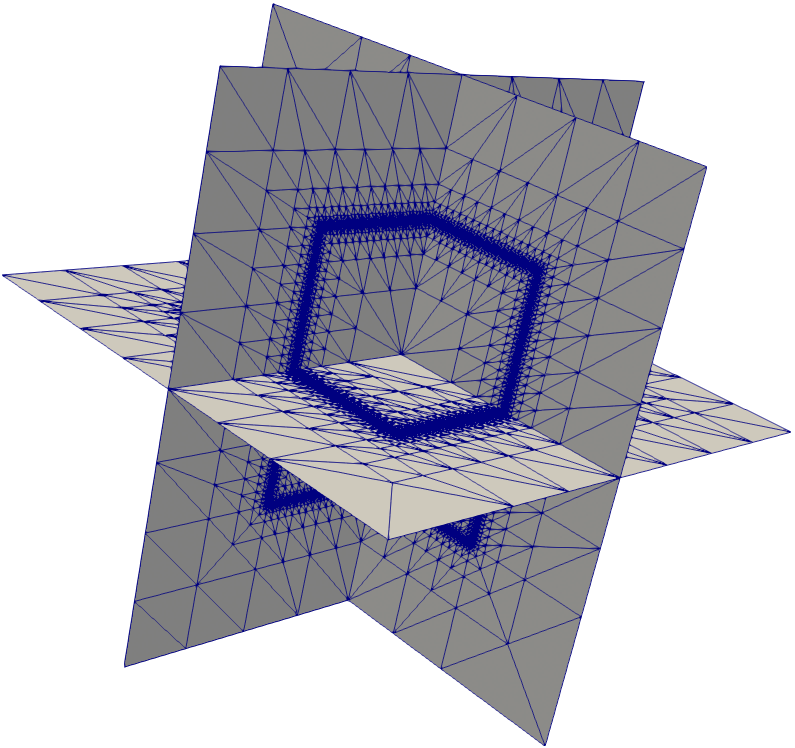
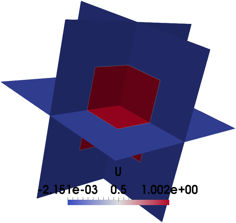
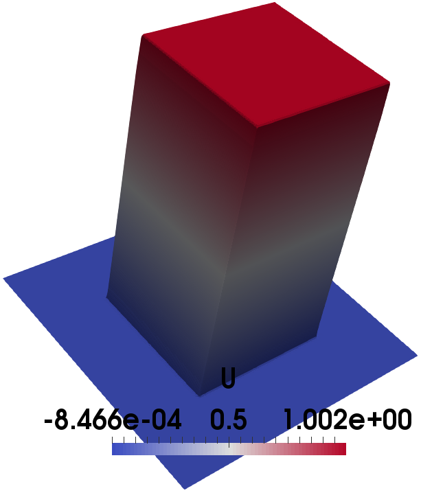
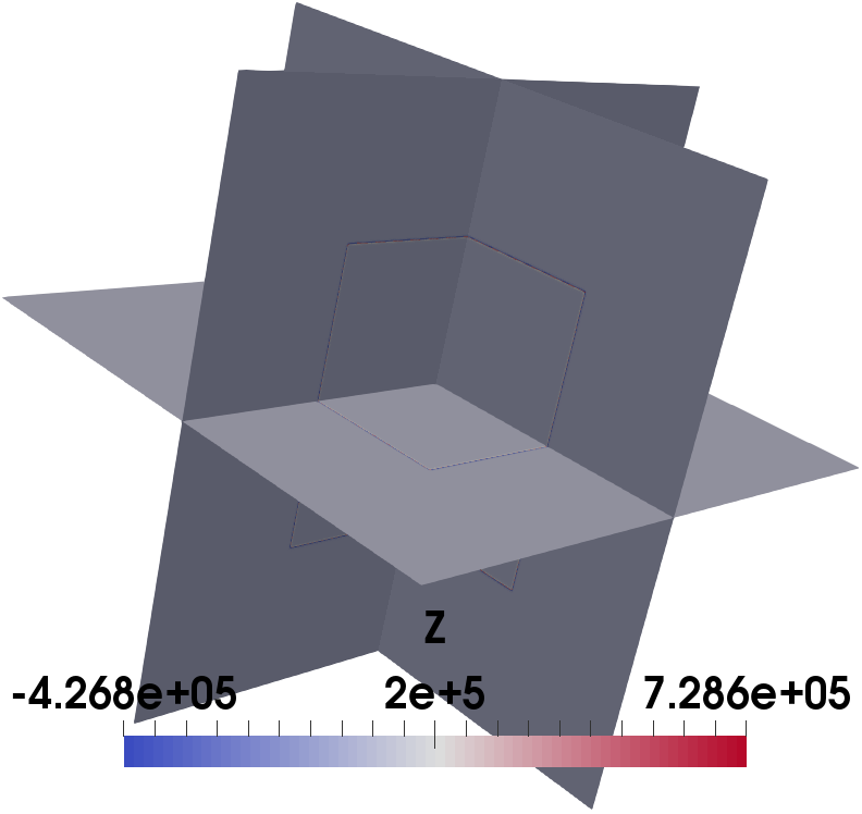
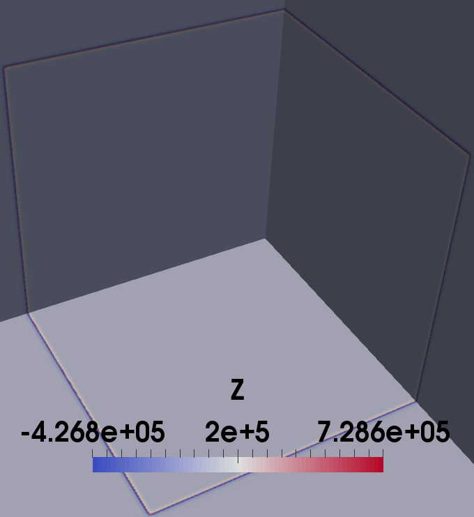
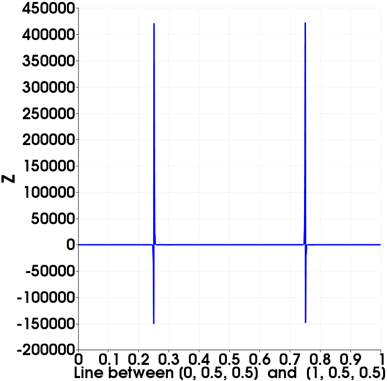
Figure 1: Example 4.2: Adaptive meshes at the $21$th refinement step with $1,895,056$ Dofs, $u_{\varrho h}$ in $\Omega$ and on the cutting plane $x_{3}=0.5$ (up), control in $\Omega$, near the interface, and on the line between $[0,0.5,0.5]$ and $[1,0.5,0.5]$ (down), $\varrho=10^{-6}$.

$\varrho$	$\|\bar{u}-u_{\varrho h}\|_{H^{-1}(\Omega)}^{2}$	eoc	$\|\bar{u}-u_{\varrho h}\|_{L^{2}(\Omega)}^{2}$	eoc
$10{{}^{0}}$	$2.1308$e$-3$		$1.2018$e$-1$
$10{{}^{-1}}$	$1.3401$e$-3$	$0.20$	$9.0747$e$-2$	$0.12$
$10{{}^{-2}}$	$1.9101$e$-4$	$0.85$	$3.6563$e$-2$	$0.39$
$10{{}^{-3}}$	$9.0010$e$-6$	$1.33$	$1.1894$e$-2$	$0.49$
$10{{}^{-4}}$	$3.1821$e$-7$	$1.45$	$3.8028$e$-3$	$0.50$
$10{{}^{-5}}$	$1.0474$e$-8$	$1.48$	$1.2075$e$-3$	$0.50$
$10{{}^{-6}}$	$3.3491$e$-10$	$1.50$	$3.7988$e$-4$	$0.50$

Table 6: Example 4.2: Errors $\|\bar{u}-u_{\varrho h}\|_{H^{-1}(\Omega)}^{2}$ and $\|\bar{u}-u_{\varrho h}\|_{L^{2}(\Omega)}^{2}$ of the approximations $u_{\varrho h}$ to the target $\bar{u}\in H^{1/2-\varepsilon}(\Omega)$.

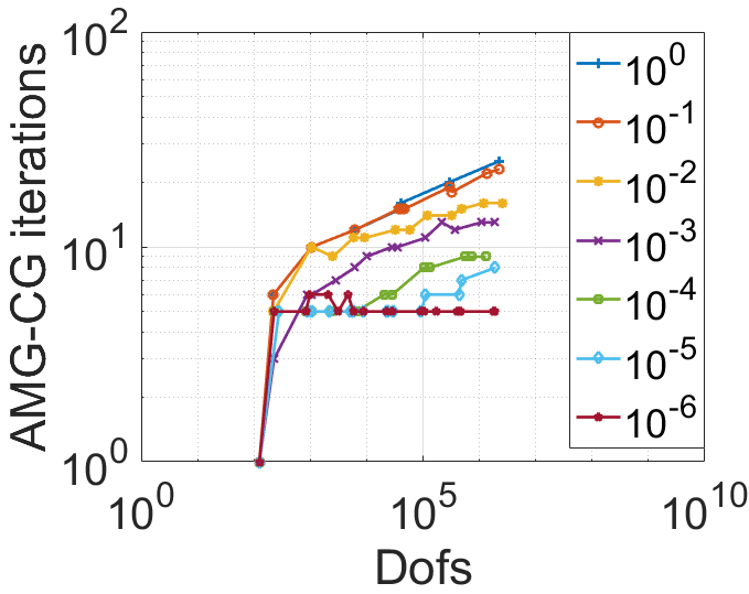
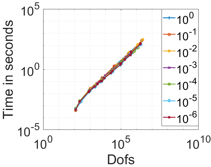
Figure 2: Example 4.2: Number of AMG preconditioned CG iterations (left) and computational time in seconds (right) with respect to different $\varrho\in\{10^{0},10^{-1},...10^{-6}\}$.

	$32$	$64$	$128$	$256$	#Dofs
$10{{}^{0}}$	37 (60.77 s)	46 (24.34 s)	42 (8.20 s)	52 (5.02 s)	$2,210,254$
$10^{-1}$	42 (66.85 s)	45 (24.85 s)	46 (9.28 s)	43 (4.64 s)	$2,278,661$
$10^{-2}$	34 (60.06 s)	38 (23.86 s)	42 (9.75 s)	43 (4.79 s)	$2,537,773$
$10^{-3}$	35 (40.92 s)	39 (15.35 s)	35 (5.12 s)	40 (3.23 s)	$1,853,354$
$10^{-4}$	33 (16.79 s)	31 (6.30 s)	39 (3.17 s)	36 (1.53 s)	$1,301,825$
$10^{-5}$	33 (17.63 s)	33 (7.65 s)	33 (3.28 s)	38 (1.88 s)	$1,910,829$
$10^{-6}$	36 (18.30 s)	37 (8.42 s)	35 (3.31 s)	44 (1.93 s)	$1,895,056$

Table 7: Example 4.2: Number of BDDC preconditioned CG iterations, solving time measured in second (s) with respect to the number of subdomains $p$ (= number of cores), regularization parameter $\varrho$, and different adaptive meshes (#Dofs).

4.3 Smooth target with non-zero boundary conditions

In the third example, we use the smooth target

$$\bar{u}(x_{1},x_{2},x_{3})=1+\sin(\pi x_{1})\sin(\pi x_{2})\sin(\pi x_{3})$$

considered in [22]. This target violates the homogeneous Dirichlet boundary conditions. As in the previous example, we solve the equation on adaptively refined meshes, which results in many local refinements near the boundary, where the control concentrates. For an illustration, we visualize the adaptive mesh, the state $u_{\varrho h}$, and the control $z_{\varrho h}$ in Fig. 3. Further, we observe the convergence order $\sqrt{1.5}$ for the approximation in $H^{-1}(\Omega)$, and $\sqrt{0.5}$ in $L^{2}(\Omega)$ with respect to $\varrho$; see Table 8. Since $\bar{u}\in C^{\infty}(\overline{\Omega})$, but $\bar{u}\notin H_{0}^{1}(\Omega)$, we only expect a reduced order of convergence for this example; see also [22, Table 7]. In Fig. 4, for each $\varrho$, we visualize the number of AMG preconditioned CG iterations (left plot) and the computational time in seconds (right plot) during the adaptive refinement levels. The AMG preconditioned CG iterations are in a small range between $1$ and $20$. The computational time scales well with respect to the number of unknowns. To see the performance of the BDDC preconditioner with respect to an adaptive refinement, we select similar numbers of Dofs for all regularization parameters, i.e., #Dofs=2,146,491 ($\varrho=10^{0}$), #Dofs=2,146,689 ($\varrho=10^{-1}$), #Dofs=2,146,575 ($\varrho=10^{-2}$), #Dofs=2,654,801 ($\varrho=10^{-3}$), #Dofs=1,997,688 ($\varrho=10^{-4}$), #Dofs=3,688,105 ($\varrho=10^{-5}$), and #Dofs=3,676,447 ($\varrho=10^{-6}$). Table 9 presents the number of BDDC preconditioned CG iterations, and solving times measured in second (s) with respect to the number of subdomains $p$ and the regularization parameter $\varrho$. We again observe a relatively good performance in both the number of BDDC preconditioned CG iterations and the computational time, as well as good strong scalability with respect to the number of subdomains $p$.

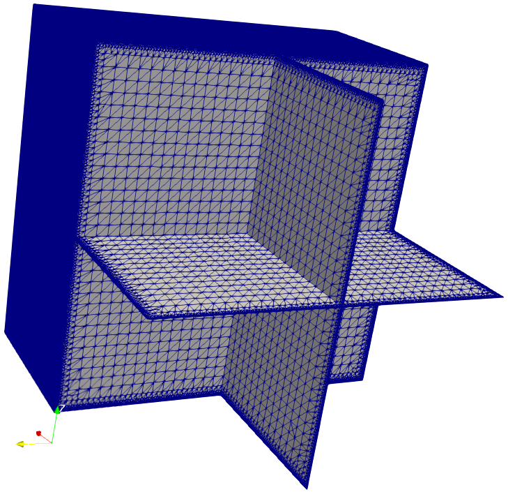
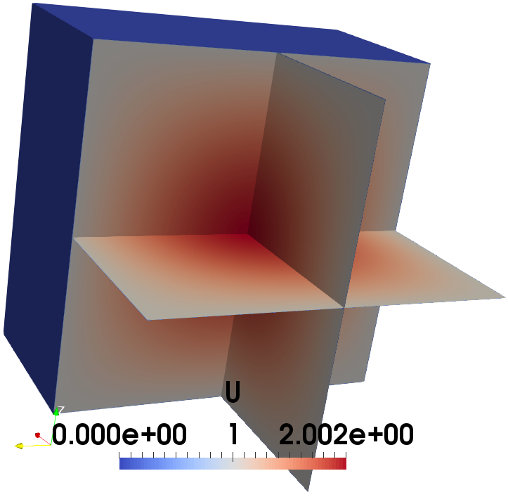
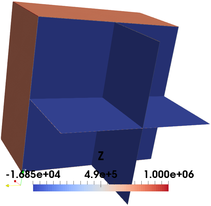
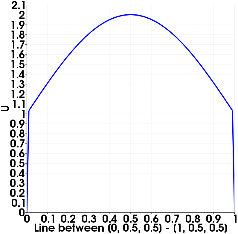
Figure 3: Example 4.3: Adaptive meshes at the $12$th refinement step with $3,688,306$ Dofs, $u_{\varrho h}$ in $\Omega$ and $z_{\varrho h}$ in $\Omega$ (up); $u_{\varrho h}$ and $z_{\varrho h}$ along the line between $[0,0.5,0.5]$ and $[1,0.5,0.5]$ (down), $\varrho=10^{-6}$.

$\varrho$	$\|\bar{u}-u_{\varrho h}\|_{H^{-1}(\Omega)}^{2}$	eoc	$\|\bar{u}-u_{\varrho h}\|_{L^{2}(\Omega)}^{2}$	eoc
$10{{}^{0}}$	$3.5241$e$-2$		$1.5613$e$-0$
$10{{}^{-1}}$	$2.1590$e$-2$	$0.21$	$1.0842$e$-0$	$0.16$
$10{{}^{-2}}$	$2.5430$e$-3$	$0.93$	$3.2593$e$-1$	$0.52$
$10{{}^{-3}}$	$8.8234$e$-5$	$1.46$	$9.5243$e$-2$	$0.53$
$10{{}^{-4}}$	$2.7302$e$-6$	$1.51$	$3.0292$e$-2$	$0.50$
$10{{}^{-5}}$	$8.5525$e$-8$	$1.50$	$9.6709$e$-3$	$0.50$

Table 8: Example 4.3: Errors $\|\bar{u}-u_{\varrho h}\|_{H^{-1}(\Omega)}^{2}$ and $\|\bar{u}-u_{\varrho h}\|_{L^{2}(\Omega)}^{2}$ of the approximations $u_{\varrho h}$ to the target $\bar{u}\in C^{\infty}(\overline{\Omega}$, $\bar{u}\notin H_{0}^{1}(\Omega)$.

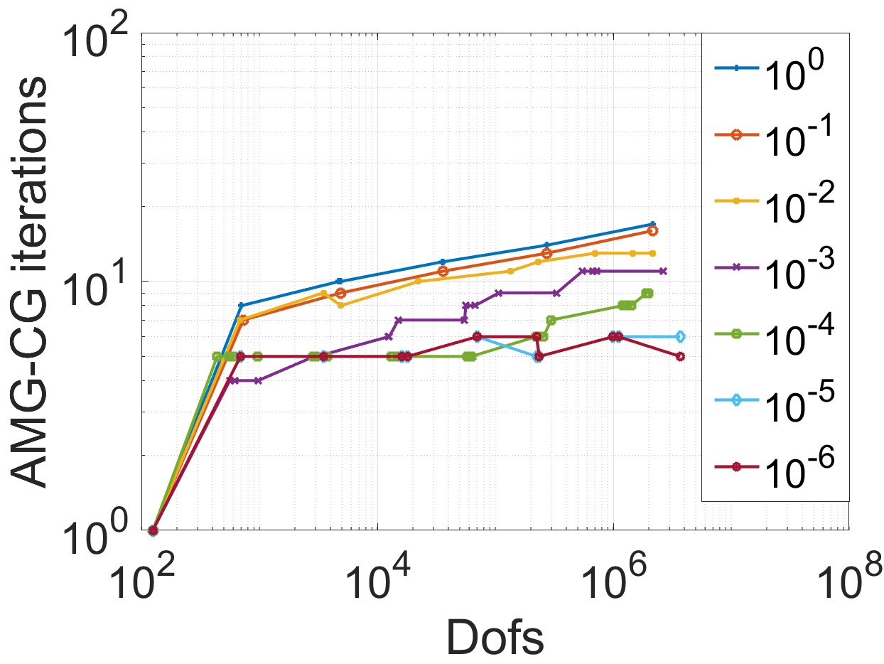
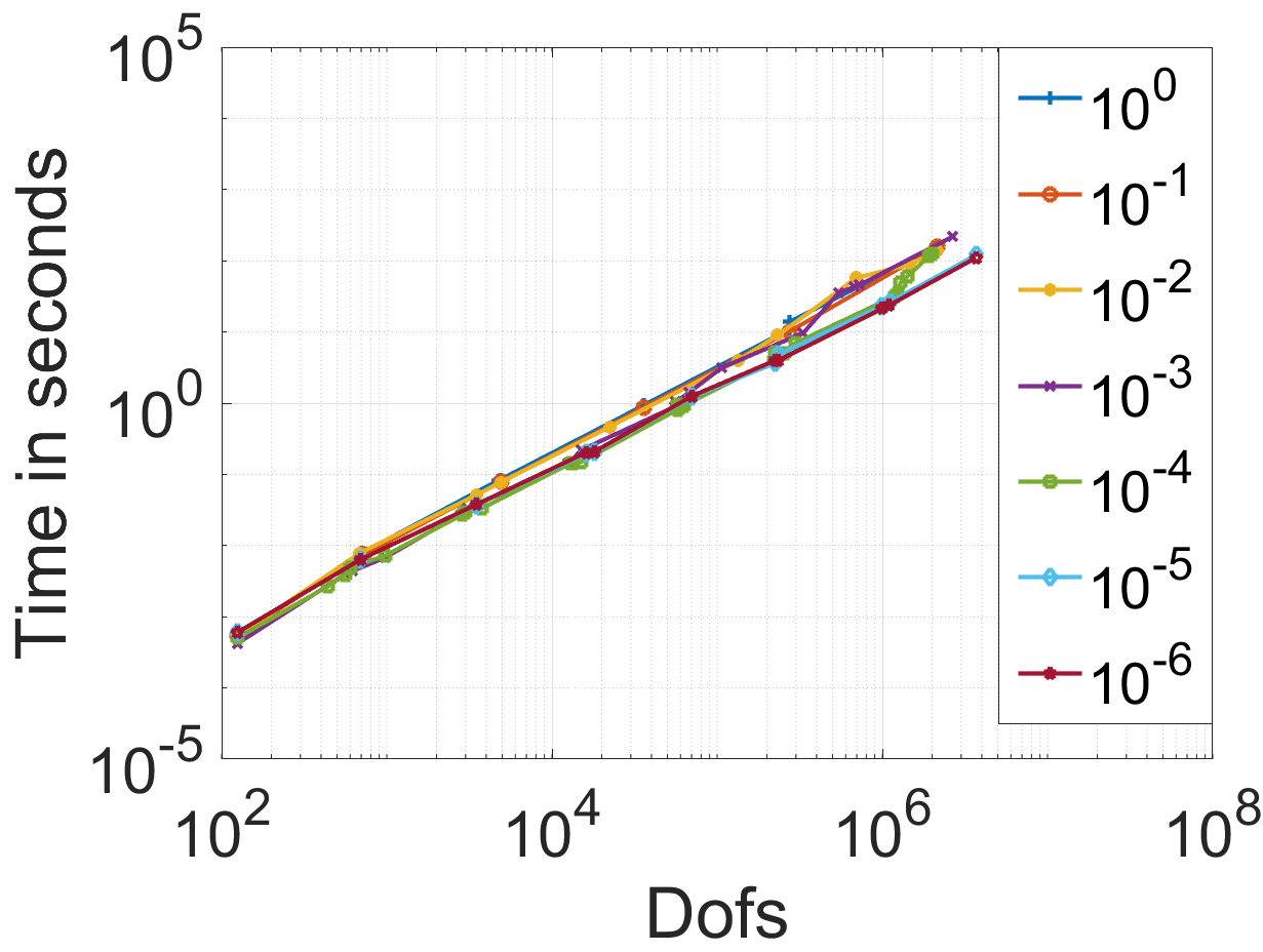
Figure 4: Example 4.3: Number of AMG preconditioned CG iterations (left) and computational time in seconds (right) with respect to different
$\varrho\in\{10^{0},10^{-1},...10^{-6}\}$.

	$32$	$64$	$128$	$256$	#Dofs
$10{{}^{0}}$	33 (45.61 s)	32 (15.37 s)	32 (5.62 s)	33 (2.78 s)	$2,146,491$
$10^{-1}$	30 (41.51 s)	31 (15.16 s)	32 (5.71 s)	32 (2.84 s)	$2,146,689$
$10^{-2}$	30 (42.13 s)	31 (15.46 s)	30 (5.14 s)	32 (2.59 s)	$2,146,575$
$10^{-3}$	29 (32.46 s)	34 (14.30 s)	32 (7.20 s)	39 (3.27 s)	$2,654,801$
$10^{-4}$	29 (15.87 s)	31 (6.98 s)	31 (2.94 s)	29 (1.40 s)	$1,997,688$
$10^{-5}$	30 (21.03 s)	30 (9.22 s)	33 (4.34 s)	37 (2.73 s)	$3,688,105$
$10^{-6}$	31 (22.57 s)	33 (10.06 s)	31 (4.05 s)	38 (2.57 s)	$3,676,447$

Table 9: Example 4.3: Number of BDDC preconditioned CG iterations, solving time measured in second (s) with respect to the number of subdomains $p$ (= number of cores), regularization parameter $\varrho$, and different adaptive meshes (#Dofs).

5 Conclusions

Using estimates for the error between the exact solution $u_{\varrho}$ of the optimal control problem (1) and the target $\overline{u}$ in terms of the regularization parameter $\varrho$, derived in [22], we have investigated the error between the finite element solution $u_{\varrho h}$ and the target $\overline{u}$ in terms of $\varrho$ and $h$. Furthermore, we have studied AMG and BDDC preconditioned CG solvers for (adaptive) finite element equations arising from the elliptic optimal control problem with energy regularization. Both preconditioners have shown good performance with respect to (adaptive) mesh refinements and a (decreasing) regularization parameter. Moreover, the BDDC preconditioner has shown its strong scalability with respect to the number of subdomains on a distributed memory computer.

While in this paper we have considered a distributed control problem subject to the Poisson equation, a related analysis can be done in the case of a parabolic heat equation. These results will be published elsewhere, but see [16] for a space-time discretization approach.

References

- [1] S. Badia, A. Martin, and J. Principe. Implementation and scalability analysis of balancing domain decomposition methods. Arch. Computat. Methods Eng., 20:239–262, 2013.
- [2] S. Badia, A. F. Martín, and J. Principe. Multilevel balancing domain decomposition at extreme scales. SIAM J. Sci. Comput., 38(1):C22–C52, 2016.
- [3] D. Braess. Finite Elements: Theory, Fast Solvers, and Applications in Solid Mechanics. Cambridge University Press, Cambridge, 2007.
- [4] A. Brandt, S. McCormick, and J. Ruge. Algebraic multigrid (AMG) for sparse matrix equations. In D. Evans, editor, Sparsity and its Applications, pages 257–284. Cambridge University Press, Cambridge, 1985.
- [5] W. Briggs, V. Henson, and S. McCormick. A Multigrid Tutorial. SIAM, Philadelphia, second edition, 2000.
- [6] C. Dohrmann. A preconditioner for substructuring based on constrained energy minimization. SIAM J. Sci. Comput., 25(1):246–258, 2003.
- [7] H. Goering, A. Felgenhauer, G. Lube, H. Roos, and L. Tobiska. Singularly Perturbed Differential Equations. Akademie Verlag, Berlin, 1983.
- [8] H. Goering, M. Stynes, and L. Tobiska. Robust Numerical Methods for Singularyly Perturbed Differential Equations. Springer Verlag, Berlin, 2008.
- [9] G. Haase and U. Langer. Multigrid methods: from geometrical to algebraic versions. In A. Bourlioux, M. Gander, and G. Sabidussi, editors, Modern Methods in Scientific Computing and Applications, pages 103–153. Springer Netherlands, Dordrecht, 2002.
- [10] W. Hackbusch. Multi-Grid Methods and Applications. Springer, Heidelberg, 1985.
- [11] L. Jing and O. B. Widlund. FETI-DP, BDDC, and block Cholesky methods. Int. J. Numer. Meth. Engng., 66(2):250–271, 2006.
- [12] G. Karypis and V. Kumar. A fast and high quality multilevel scheme for partitioning irregular graphs. SIAM J. Sci. Comput., 20(1):359–392, 1998.
- [13] F. Kickinger. Algebraic multi-grid for discrete elliptic second-order problems. In W. Hackbusch and G. Wittum, editors, Multigrid Methods V, pages 157–172, Berlin, Heidelberg, 1998. Springer Verlag.
- [14] J. Kraus and M. Wolfmayr. On the robustness and optimality of algebraic multilevel methods for reaction-diffusion type problems. Comput. Visual Sci., 16:15–32, 2013.
- [15] U. Langer, M. Neumüller, and A. Schafelner. Space-time finite element methods for parabolic evolution problems with variable coefficients. In T. Apel, U. Langer, A. Meyer, and O. Steinbach, editors, Advanced Finite Element Methods with Applications: Selected Papers from the 30th Chemnitz Finite Element Symposium 2017, pages 247–275. Springer International Publishing, Cham, 2019.
- [16] U. Langer, O. Steinbach, F. Tröltzsch, and H. Yang. Space-time finite element discretization of parabolic optimal control problems with energy regularization. SIAM J. Numer. Anal., 2020. accepted.
- [17] U. Langer and H. Yang. Robust and efficient monolithic fluid-structure-interaction solvers. Int. J. Numer. Meth. Engng., 108(4):303–325, 2016.
- [18] U. Langer and H. Yang. BDDC preconditioners for a space-time finite element discretization of parabolic problems. In R. Haynes, S. MacLachlan, X. Cai, L. Halpern, H. Kim, A. Klawonn, and O. Widlund, editors, Domain Decomposition Methods in Science and Engineering XXV, pages 367–374, Cham, 2020. Springer.
- [19] S. MacLachlan and N. Madden. Robust solution of singularly perturbed problems using multigrid methods. SIAM J. Sci. Comput., 35(5):A2225–A2254, 2013.
- [20] J. Mandel and C. Dohrmann. Convergence of a balancing domain decomposition by constraints and energy minimization. Numer. Linear Algebra Appl., 10(7):639–659, 2003.
- [21] J. Mandel, C. Dohrmann, and R. Tezaur. An algebraic theory for primal and dual substructuring methods by constraints. Appl. Numer. Math., 54(2):167–193, 2005.
- [22] M. Neumüller and O. Steinbach. Regularization error estimates for distributed control problems in energy spaces. Math. Meth. Appl. Sci., 2020. published online.
- [23] T. A. Nhan, S. MacLachlan, and N. Madden. Boundary layer preconditioners for finite-element discretizations of singularly perturbed reaction-diffusion problems. Numer. Algor., 79:281–310, 2018.
- [24] T. A. Nhan and N. Madden. An analysis of diagonal and incomplete Cholesky preconditioners for singularly perturbed problems on layer-adapted meshes. J. Appl. Math. Computing, 65:245–272, 2021.
- [25] M. Olshanskii and A. Reusken. On the convergence of a multigrid method for linear reaction-diffusion problems. Computing, 65:193–202, 2000.
- [26] C. Popa. Algebraic multigrid smoothing property of kaczmarz’s relaxation for general rectangular linear systems. Electron. Trans. Numer. Anal., 29:150–162, 2007-2008.
- [27] J. Ruge and K. Stüben. Algebraic multigrid. In S. McCormick, editor, Multigrid Methods, chapter 4, pages 73–130. SIAM, Philadelphia, 1987.
- [28] A. H. Schatz and L. B. Wahlbin. On the finite element method for singularly perturbed reaction-diffusion problems in two and one dimensions. Math. Comp., 40(161):47–89, 1983.
- [29] O. Steinbach. Numerical Approximation Methods for Elliptic Boundary Value Problems: Finite and Boundary Elements. Springer, 2008.
- [30] O. Steinbach. Space-time finite element methods for parabolic problems. Comput. Methods Appl. Math., 15:551–566, 2015.
- [31] O. Steinbach and H. Yang. Comparison of algebraic multigrid methods for an adaptive space-time finite-element discretization of the heat equation in 3d and 4d. Numer. Linear Algebra Appl., 25(3):e2143, 2018.
- [32] A. Toselli and O. B. Widlund. Domain Decomposition Methods — Algorithms and Theory. Springer, Berlin, Heidelberg, 2005.
- [33] R. Verfürth. A posteriori error esimtation techniques for finite element methods. Oxford University Press, Oxford, 2013.
- [34] J. Xu and L. Zikatanov. Algebraic multigrid methods. Acta Numer., 26:591–721, 2017.
- [35] H. Yang and W. Zulehner. Numerical simulation of fluid-structure interaction problems on hybrid meshes with algebraic multigrid methods. J. Comput. Appl. Math., 235(18):5367–5379, 2011.
- [36] S. Zampini and X. Tu. Multilevel balancing domain decomposition by constraints deluxe algorithms with adaptive coarse spaces for flow in porous media. SIAM J. Sci. Comput., 39(4):A1389–A1415, 2017.