Solving Fredholm second-kind integral equations with singular right-hand sides on non-smooth boundaries

Abstract

A numerical scheme is presented for the solution of Fredholm second-kind boundary integral equations with right-hand sides that are singular at a finite set of boundary points. The boundaries themselves may be non-smooth. The scheme, which builds on recursively compressed inverse preconditioning (RCIP), is universal as it is independent of the nature of the singularities. Strong right-hand-side singularities, such as $1/|r|^{\alpha}$ with $\alpha$ close to $1$, can be treated in full machine precision. Adaptive refinement is used only in the recursive construction of the preconditioner, leading to an optimal number of discretization points and superior stability in the solve phase. The performance of the scheme is illustrated via several numerical examples, including an application to an integral equation derived from the linearized BGKW kinetic equation for the steady Couette flow.

1 Introduction

Fredholm second-kind integral equations (SKIEs) have become standard tools for solving boundary value problems of elliptic partial differential equations [9, 23, 26, 30, 32]. Advantages include dimensionality reduction in the solve phase, elimination of the need to impose artificial boundary conditions for exterior problems, easily achieved high-order discretization, and optimal complexity when coupled with fast algorithms such as the fast multipole method [14].

The present work is about the numerical solution to SKIEs of the form

$$(I+K)\rho(r)=f(r)\,,\quad r\in\Gamma\,.$$ (1)

Here $r\in\mathbb{R}^{2}$ is a point in the plane; $I$ is the identity operator; $\rho$ is an unknown layer density to be solved for; $\Gamma$ is a piecewise smooth closed contour (boundary) with a finite number of corners; $K$ is an integral operator on $\Gamma$ which is compact away from the corners; and $f$ is a right-hand side which is singular at a finite number of boundary points, which may or may not coincide with the corner vertices, but otherwise smooth. The union of corner vertices and boundary points where $f$ is singular is referred to as singular points. These points are denoted $\gamma_{j}$, $j=1,2,\ldots$. The kernel of $K$ is denoted $K(r,r^{\prime})$. We also assume a parameterization $r(s)$ of $\Gamma$ where $s$ is a parameter.

We shall construct an efficient scheme for the numerical solution of (1). The difficulty in this undertaking is that the singularities in $f$ and the non-compactness of $K$ at the $\gamma_{j}$ may require a very large number of unknowns for the resolution of $\rho$. This, in turn, may lead to high computing costs and also to artificial ill-conditioning and reduced achievable precision in quantities computed from $\rho$.

The nature of the singularity of $f$ can be rather arbitrary in the applications we consider. There is no analysis of $f$ involved in our work and neither is there any further analysis of $K$. We only assume that $f$ can be evaluated everywhere at $\Gamma$ except for at the $\gamma_{j}$. If, however, it is known whether the leading singular behavior of $f$ is homogeneous on $\Gamma$ in the shape of a wedge and whether $K$ is scale invariant on such $\Gamma$, that information can be used to further improve the performance of our scheme.

We shall solve (1) numerically using Nyström discretization based on underlying composite $16$-point Gauss-Legendre quadrature and the parameterization $r(s)$ and then accelerate and stabilize the solution process using an extended version of the recursively compressed inverse preconditioning (RCIP) method [16]. The discretization is chiefly done on a coarse mesh with quadrature panels of approximately equal size. The coarse quadrature panels are chosen so that the following holds: all singular points $\gamma_{j}$ coincide with panel endpoints; for $r$ on a panel close to $\gamma_{j}$ and $r^{\prime}$ away from $\gamma_{j}$, $K(r(s),r^{\prime})$ is smooth; for $r$ away from $\gamma_{j}$ and $r^{\prime}$ on a panel close to $\gamma_{j}$, $K(r,r^{\prime}(s))$ is smooth.

The RCIP method assumes that the SKIE has a panelwise smooth right-hand side and consists of the following steps:

• Transform the SKIE at hand into a form where the layer density to be solved for is panelwise smooth.

• Use Nyström discretization to discretize the transformed SKIE on a grid on a fine mesh, obtained from the coarse mesh by repeated subdivision of the panels closest to each $\gamma_{j}$.

• Compress the transformed and discretized SKIE so that it can be solved on a grid on the coarse mesh without the loss of information. This involves the use of a forward recursion.

• Solve the compressed equation.

• Reconstruct the solution to the original SKIE from the solution to the compressed equation. This involves the use of a backward recursion.

In this paper, we extend the RCIP method to treat singular right-hand sides. The method is universal since algorithmic steps are completely independent of the nature of the singularities in the right-hand-side function. The only information needed is the locations of singularities. Very strong singularities can be treated in full machine precision. Indeed, we have studied singularities of the form $1/|r|^{\alpha}$ for a wide range of $\alpha$ and our method works very well even for $\alpha=1+0.3{\rm i}$.

We further observe that problems involving sources close to corners occur surprisingly often in computational electromagnetics and computational fluid dynamics. Examples include the determination of radiation patterns from 5G base stations placed at street corners [33] and singularity formation in Hele–Shaw flows driven by multipoles [31]. These problems involve nearly singular right-hand sides and can be treated easily by the method developed in this paper. The 5G base stations often have antennas with logarithmic singularities in their radiated field.

Examples of problems involving singular sources close to smooth surfaces can be found in the area of Internet of Things (IoT), where the radiation patterns from antennas, integrated in devices, again need to be found numerically for design purposes [10]. The most common types of IoT antennas are stripline and patch antennas. These have a radiating current density very close to a metallic ground plane, which often is a smooth part of the housing of the device. As IoT carrier frequencies get higher, antennas become smaller and the distance between the current and the housing surface shrinks – leading to increased need for computational resolution.

The paper is organized as follows. In Section 2, a new transformation is introduced to treat the singular right-hand side $f$. Sections 3, 4, 5, and 6 present detailed modifications to the other steps in the list that follow from the introduction of the new transform. Numerical examples are presented in Section 7. Finally, we discuss the application of our new method to the integral equation derived from the linearized Bhatnagar-Gross-Krook-Welander (BGKW) kinetic equation [5, 35] for the steady Couette flow.

In order to keep the presentation concise, we concentrate on new development and refer the reader to the recently updated compendium [16] for details on the RCIP method. This compendium, in turn, contains references to original journal papers.

2 Transformed equation with smooth density

This section reviews the original RCIP transformation, discusses its shortcomings for singular right-hand sides $f$, and presents a new and better transformation. We frequently use the concept of panelwise smooth functions. By this we mean functions which can be well approximated by polynomials of degree $15$ in $s$ on individual quadrature panels. We also introduce the boundary subsets $\Gamma^{j\star}$, which refer to the four panels that are closest to a point $\gamma_{j}$ (two on each side), and the boundary subsets $\Gamma^{j\star\star}$, which refer to the two panels that are closest to a point $\gamma_{j}$ (one on each side).

2.1 The original transformation

The original RCIP transformation for SKIEs of the form (1) assumes that $f$ is a panelwise smooth function and relies on a kernel split

$$K(r,r^{\prime})=K^{\star}(r,r^{\prime})+K^{\circ}(r,r^{\prime})\,,\quad r,r^{\prime}\in\Gamma\,,$$ (2)

and a corresponding operator split

$$K=K^{\star}+K^{\circ}\,.$$ (3)

In (3), the operator $K^{\star}$ denotes the part of $K$ that accounts for self-interaction close to the corner vertices $\gamma_{j}$, and $K^{\circ}$ is the compact remainder. The split (2) is determined from a geometric criterion: if $r$ and $r^{\prime}$ both are in $\Gamma^{j\star}$ for some $j$, then $K^{\star}(r,r^{\prime})=K(r,r^{\prime})$. Otherwise $K^{\star}(r,r^{\prime})$ is zero.

The change of variables

$$\rho(r)=(I+K^{\star})^{-1}\tilde{\rho}(r)\,,\quad r\in\Gamma\,,$$ (4)

makes (1) with (3) assume the form

$$(I+K^{\circ}(I+K^{\star})^{-1})\tilde{\rho}(r)=f(r)\,,\quad r\in\Gamma\,.$$ (5)

When $f$ is panelwise smooth, the transformed layer density $\tilde{\rho}$ in (5) will, loosely speaking, also be panelwise smooth. This is so since the action of $K^{\circ}$ on any function results in a panelwise smooth function. In particular, $\tilde{\rho}$ will be smooth on $\Gamma^{j\star\star}$. The panelwise smoothness of $\tilde{\rho}$ on $\Gamma^{j\star\star}$, inherited from $f$, is the key property which makes the transformed equation (5) efficient for the original problem (1). The efficiency comes from the fact that a panelwise smooth unknown is easy to resolve by panelwise polynomials.

2.2 A new transformation

When the right-hand side $f$ in (1) is not panelwise smooth, but has singularities at the corner vertices, the transformed layer density $\tilde{\rho}$ in (5) is not panelwise smooth either. In order to fix this problem we now propose a new transformation of (1) which, in addition to the split of $K$, also splits the right-hand side $f$ and the unknown $\rho$ as

$$f(r) =f^{\star}(r)+f^{\circ}(r)\,,\quad r\in\Gamma\,,$$ (6)

$$\rho(r) =v(r)+g(r)\,,\quad r\in\Gamma\,.$$ (7)

Here $f^{\star}(r)=f(r)$ if $r\in\Gamma^{j\star}$ for some $j$. Otherwise $f^{\star}(r)$ is zero. The functions $v$ and $g$ are given by

$$v(r) =(I+K^{\star})^{-1}\tilde{v}(r)\,,$$ (8)

$$g(r) =(I+K^{\star})^{-1}f^{\star}(r)\,,$$ (9)

where $\tilde{v}$ is a new unknown transformed layer density.

Use of (3), (6), (7), (8), and (9) makes (1) assume the form

$$(I+K^{\circ}(I+K^{\star})^{-1})\tilde{v}(r)=f^{\circ}(r)-K^{\circ}(I+K^{\star})^{-1}f^{\star}(r)\,,\quad r\in\Gamma\,.$$ (10)

One can see, in (10), that $\tilde{v}$ is panelwise smooth on $\Gamma^{j\star\star}$. This is so since the right-hand side of (10) is smooth on $\Gamma^{j\star}$.

We remark that if $\Gamma$ is smooth so that there are no corners, only singularities in $f$, then the local transformation (8) is not needed and (10) reduces to

$$(I+K)v(r)=f^{\circ}(r)-K^{\circ}(I+K^{\star})^{-1}f^{\star}(r)\,,\quad r\in\Gamma\,.$$ (11)

One can also imagine mixed situations where (8) is used only at those $\gamma_{j}$ which correspond to corner vertices.

3 Discretization of (5) and (10)

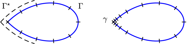
Figure 1: A contour $\Gamma$ with a corner at $\gamma$ of opening angle $\theta=\pi/2$. Left: A coarse mesh with ten quadrature panels on $\Gamma$. A subset of $\Gamma$, called $\Gamma^{\star}$, covers the four coarse panels closest to $\gamma$. Right: A fine mesh created from the coarse mesh by subdividing the panels closest to $\gamma$ a number $n_{\rm sub}=3$ of times.

This section summarizes the modifications needed in the RCIP method in order for it to apply to (10) rather than to (5). We first show how RCIP is applied to (5), with detailed references to [16], and then state the modifications needed for (10). For simplicity of presentation it is from now on assumed that there is only one singular point, denoted $\gamma$, with an associated four-panel neighboring zone denoted $\Gamma^{\star}$ as illustrated in Figure 1. We let $\Gamma^{\star\star}$ refer to the two panels closest to $\gamma$ (one on each side).

The discretization of (5) takes place on two different meshes: on the coarse mesh and on a fine mesh. The fine mesh is constructed from the coarse mesh by $n_{\rm sub}$ times subdividing the panels closest to $\gamma$. See the right image of Figure 1 for an example. Discretization points on the coarse mesh constitute the coarse grid. Points on the fine mesh constitute the fine grid. The number of refinement levels, $n_{\rm sub}$, is chosen so that the operator $(I+K^{\star})^{-1}$ in (5) is resolved to a desired precision.

As mentioned in Section 1, our Nyström discretization relies on composite 16-point Gauss–Legendre quadrature. This means that an integral

$$\int_{\Gamma}h(r)\,{\rm d}\ell\,,$$

where $h$ is a smooth function and ${\rm d}\ell$ is an element of arc length, can be approximated by a sum on the coarse grid

$$\int_{\Gamma}h(r)\,{\rm d}\ell\approx\sum_{j}h(r(s_{{\rm coa}_{j}}))\lvert\dot{r}(s_{{\rm coa}_{j}})\rvert w_{{\rm coa}_{j}}\,.$$ (12)

Here $\dot{r}(s)={\rm d}r(s)/{\rm d}s$ denotes differentiation with respect to the boundary parameter $s$ and $w_{{\rm coa}_{j}}$ are appropriately scaled Gauss–Legendre weights. A formula, analogous to (12) but with subscripts coa replaced with subscripts fin, holds when $h$ is a singular function that needs the fine grid for resolution.

3.1 Smooth right-hand side

It is shown in [16, Appendix B] that the discretization of (5) on the fine grid followed by RCIP-style compression leads to the system

$$\left({\bf I}_{\rm coa}+{\bf K}_{\rm coa}^{\circ}{\bf R}\right)\tilde{\boldsymbol{\rho}}_{\rm coa}={\bf f}_{\rm coa}\,.$$ (13)

Here ${\bf R}$ is a block-diagonal matrix defined as [16, Eq. (26)]

$${\bf R}={\bf P}_{W}^{\rm T}\left({\bf I}_{\rm fin}+{\bf K}_{\rm fin}^{\star}\right)^{-1}{\bf P}\,,$$ (14)

and the subscripts coa and fin indicate what type of mesh is used for discretization. The prolongation matrix ${\bf P}$ interpolates piecewise polynomial functions known at the coarse grid to the fine grid. The weighted prolongation matrix ${\bf P}_{W}$ resembles ${\bf P}$, but is designed to act on discretized functions multiplied by quadrature weights [16, Eq. (21)]. The interpolation is done with respect to the boundary parameter $s$. The superscript T denotes the transpose.

3.2 Singular right-hand side

The discretization and compression of (10) can be constructed in a manner completely analogous to that of (5) and leads to the system

$$({\bf I}_{\rm coa}+{\bf K}_{\rm coa}^{\circ}{\bf R})\tilde{\bf v}_{\rm coa}={\bf f}^{\circ}_{\rm coa}-{\bf K}_{\rm coa}^{\circ}{\bf R}_{f}{\bf f}^{\star}_{\rm coa}\,,$$ (15)

where ${\bf R}$ is as in (14) and

$${\bf R}_{f}={\bf P}_{W}^{\rm T}\left({\bf I}_{\rm fin}+{\bf K}_{\rm fin}^{\star}\right)^{-1}{\bf P}_{f}\,.$$ (16)

The prolongation matrix ${\bf P}_{f}$ interpolates $f$ from the coarse grid to the fine grid and can easily be constructed from computed values of $f$ on the two grids respectively. The matrix ${\bf P}_{f}$ is block-diagonal with blocks being either identity matrices or, for entries corresponding to discretization points on $\Gamma^{\star\star}$, the rectangular rank-one matrix

$${\bf P}_{f}^{\star\star}=\frac{1}{{\bf f}_{\rm coa}^{\star\star{\rm H}}{\bf f}_{\rm coa}^{\star\star}}{\bf f}^{\star\star}_{\rm fin}{\bf f}^{\star\star{\rm H}}_{\rm coa}\,.$$ (17)

Here ${\bf f}_{\rm fin}^{\star\star}$ is a column vector with values of $f$ on the fine grid on $\Gamma^{\star\star}$, ${\bf f}_{\rm coa}^{\star\star}$ is a column vector with values of $f$ on the coarse grid on $\Gamma^{\star\star}$, and H denotes the conjugate transpose. Clearly, ${\bf P}_{f}^{\star\star}{\bf f}_{\rm coa}^{\star\star}={\bf f}_{\rm fin}^{\star\star}$.

4 Forward recursion for ${\bf R}$ and ${\bf R}_{f}$

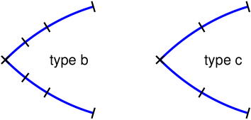
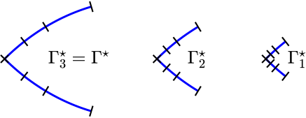
Figure 2: Top row: meshes of type b and type c on the boundary subset $\Gamma^{\star}$. The type b mesh has six panels. The type c mesh has four panels. Bottom row: the boundary subsets $\Gamma_{3}^{\star}=\Gamma^{\star}$, $\Gamma_{2}^{\star}$, and $\Gamma_{1}^{\star}$ along with their corresponding type b meshes for $n_{\rm sub}=3$.

The matrices ${\bf R}$ and ${\bf R}_{f}$ of (14) and (16) differ from the identity matrix only in that they each contain a non-trivial $64\times 64$ diagonal block, associated with entries corresponding to discretization points on $\Gamma^{\star}$. These diagonal blocks can be efficiently constructed via recursions relying on the discretization of $K$ on small meshes on a hierarchy of boundary subsets $\Gamma_{i}^{\star}$ around $\gamma$. Central to the recursions are two types of overlapping meshes called type b and type c. The type b mesh contains six quadrature panels. The type c mesh contains four quadrature panels. See Figure 2 for an illustration and [16, Section 7] for more information.

The recursions for ${\bf R}$ and ${\bf R}_{f}$, given below, use local prolongation matrices ${\bf P}_{\rm bc}$, ${\bf P}_{W{\rm bc}}$, and ${\bf P}_{fi{\rm bc}}$ similar to the global matrices ${\bf P}$, ${\bf P}_{W}$ and ${\bf P}_{f}$ of Section 3. The matrix ${\bf P}_{\rm bc}$ performs polynomial interpolation from a grid on a type c mesh to a grid on a type b mesh on the same level. The matrix ${\bf P}_{fi{\rm bc}}$ interpolates $f$ from a grid on a type c mesh to a grid on a type b mesh on the same level. The subscript $i$ indicates that ${\bf P}_{fi{\rm bc}}$ depends on the hierarchical level in which it appears.

The matrices ${\bf P}_{\rm bc}$ and ${\bf P}_{W{\rm bc}}$ are level independent. Their construction is described in [16, Section 7.1]. The matrix ${\bf P}_{fi{\rm bc}}$ is constructed analogously to the matrix ${\bf P}_{f}$ of Section 3.

4.1 The recursion for ${\bf R}$

It is shown in [16, Appendix D] that the non-trivial diagonal $64\times 64$ block of ${\bf R}$ can be obtained from the recursion

$${\bf R}_{i}={\bf P}^{T}_{W\rm{bc}}\left(\mathbb{F}\{{\bf R}_{i-1}^{-1}\}+{\bf I}_{\rm b}^{\circ}+{\bf K}_{i{\rm b}}^{\circ}\right)^{-1}{\bf P}_{\rm{bc}}\,,\quad i=1,\ldots,n_{\rm sub}\,,$$ (18)

with the initializer

$$\mathbb{F}\{{\bf R}_{0}^{-1}\}={\bf I}_{\rm b}^{\star}+{\bf K}^{\star}_{1{\rm b}}\,.$$ (19)

Here ${\bf K}_{i{\rm b}}$ is the discretization of $K$ on a type b mesh on level $i$ in the hierarchy of local meshes around $\gamma$. The operator $\mathbb{F}\{\cdot\}$ expands its matrix argument by zero-padding (adding a frame of zeros of width 16 around it). The superscripts $\star$ and $\circ$ denote matrix splits analogous to the split (3).

The forward recursion (18) starts at the finest refinement level, $i=1$, and ascends through the hierarchy of levels until it reaches the coarsest level $i=n_{\rm sub}$. The matrix ${\bf R}_{n_{\rm sub}}$ is equal to the non-trivial $64\times 64$ block of ${\bf R}$.

4.2 The recursion for ${\bf R}_{f}$

A recursion for the non-trivial $64\times 64$ block of ${\bf R}_{f}$ can be derived in complete analogy with the derivation of (18). See A for the key steps of the derivation. The result is

$${\bf R}_{fi}={\bf P}_{W{\rm bc}}^{T}\left(\mathbb{F}\{{\bf R}_{i-1}^{-1}\}+{\bf I}_{\rm b}^{\circ}+{\bf K}_{i{\rm b}}^{\circ}\right)^{-1}\left(\mathbb{F}\{{\bf R}_{i-1}^{-1}{\bf R}_{f(i-1)}\}+{\bf I}_{\rm b}^{\circ}\right){\bf P}_{fi{\rm bc}}\,,\\ \quad i=1,\ldots,n_{\rm sub}\,.$$ (20)

The recursion (20) can be initialized with

$${\bf R}_{f0}={\bf R}_{0}$$ (21)

and run in tandem with (18).

4.3 Further improvement of the recursions

From (15) it is evident that the matrix ${\bf R}_{f}$ acts only on one particular known vector, namely on ${\bf f}^{\star}_{\rm coa}$. Therefore, rather than first finding ${\bf R}_{f}$ via (20) and then computing the vector

$${\bf r}_{f}^{\star}={\bf R}_{f}{\bf f}^{\star}_{\rm coa}\,,$$ (22)

one can instead modify (20) with (21) so that it produces ${\bf r}_{f}^{\star}$ directly

$${\bf r}_{fi}^{\star}={\bf P}_{W{\rm bc}}^{T}\left(\mathbb{F}\{{\bf R}_{i-1}^{-1}\}+{\bf I}_{\rm b}^{\circ}+{\bf K}_{i{\rm b}}^{\circ}\right)^{-1}\left(\mathbb{F}\{{\bf R}_{i-1}^{-1}{\bf r}_{f(i-1)}^{\star}\}+{\bf f}_{i{\rm b}}^{\circ}\right)\,,$$

$$\hskip 252.94499pti=1,\ldots,n_{\rm sub}\,,$$ (23)

$${\bf r}_{f0}^{\star}={\bf R}_{f0}{\bf f}_{1{\rm b}}^{\star}\,.$$ (24)

The recursion (23) with (24) is a bit faster than (20) with (21).

It is also worth noting that all three recursions (18), (20), and (23) can be implemented without the explicit inversion of ${\bf R}_{i-1}$. The key to this is to use the Schur–Banachiewicz inverse formula for partitioned matrices [21, Eq. (8)]. Avoiding inversion is particularly important when ${\bf R}_{i-1}$ is ill conditioned. Details on an implementation for (18), free from inversion of ${\bf R}_{i-1}$, are given in [16, Section 8] (see also B).

4.4 Efficient initializers

A minor problem with the recursions (18), (20), and (23) is that it could be difficult to determine a suitable recursion length $n_{\rm sub}$ a priori. A too large $n_{\rm sub}$ leads to unnecessary work. A too small $n_{\rm sub}$ fails to resolve the problem. Should it, however, happen that $K$ is scale-invariant on wedges, there may be an easy way around this problem. The key observation is that for large $n_{\rm sub}$ and at levels $i$ such that $n_{\rm sub}-i\gg 1$, the matrices ${\bf K}^{\circ}_{i{\rm b}}$ have often converged to a matrix ${\bf K}^{\circ}_{\rm b}$ (in double precision arithmetic) that is independent of $i$. This, typically, happens for $n_{\rm sub}-i>60$ and means that (18) assumes the form of a fixed-point iteration

$${\bf R}_{\ast i}={\bf P}^{T}_{W\rm{bc}}\left(\mathbb{F}\{{\bf R}_{\ast(i-1)}^{-1}\}+{\bf I}_{\rm b}^{\circ}+{\bf K}_{\rm b}^{\circ}\right)^{-1}{\bf P}_{\rm{bc}}\,,\quad i=1,2,\ldots\,.$$ (25)

It also means that all ${\bf R}_{i}$ in (18) are the same for $n_{\rm sub}-i\gg 1$. In view of the above one can replace the initializer ${\bf R}_{0}$ of (19) with the fixed-point matrix ${\bf R}_{\ast}$ obtained by running (25) until convergence. With the choice ${\bf R}_{0}={\bf R}_{\ast}$, it is enough to take $n_{\rm sub}=60$ steps in the recursion (18). See, further, the discussion in [16, Sections 12–13].

In a procedure similar to that just described, it is also possible to replace the initializers ${\bf R}_{f0}$ and ${\bf r}_{f0}^{\star}$ of (21) and (24) with more efficient initializers. The requirements are, in addition to that $K$ is scale invariant on wedges, that the leading singular behavior of $f$ is homogeneous on wedges. If this holds, and if $n_{\rm sub}-i\gg 1$, then (20) assumes the form of a linear fixed-point iteration

$${\bf R}_{f\ast i}={\bf P}_{W{\rm bc}}^{T}\left(\mathbb{F}\{{\bf R}_{\ast}^{-1}\}+{\bf I}_{\rm b}^{\circ}+{\bf K}_{\rm b}^{\circ}\right)^{-1}\left(\mathbb{F}\{{\bf R}_{\ast}^{-1}{\bf R}_{f\ast(i-1)}\}+{\bf I}_{\rm b}^{\circ}\right){\bf P}_{f{\rm bc}}\,,\\ \quad i=1,2,\ldots\,.$$ (26)

The fixed-point matrix ${\bf R}_{f\ast}$ can be found with direct methods solving a Sylvester equation. With the choices ${\bf R}_{f0}={\bf R}_{f\ast}$ and ${\bf r}_{f0}^{\star}={\bf R}_{f\ast}{\bf f}_{1{\rm b}}^{\star}$ it is enough to take $n_{\rm sub}=60$ steps in the recursions (20) and (23).

We remark that efficient initializers can be found also under more general conditions on $K$ than scale invariant on wedges. See [17, Section 5.3], for an example.

5 Computing integrals of $\rho$

Often, in applications, one is not primarily interested in the solution $\rho$ to (1) in itself. Rather, one is interested in computing functionals of $\rho$ of the type

$$q=\int_{\Gamma}h(r)\rho(r)\,{\rm d}\ell\,,$$ (27)

where $h(r)$ is a smooth function. The RCIP method offers an elegant way to do this that only involves quantities appearing in the compressed equations (13) and (15).

Assume that $f$ is smooth and consider (13). The quantity $q$ of (27) can then be well approximated by the sum on the coarse grid

$$q\approx\sum_{j}h(r(s_{{\rm coa}_{j}}))\hat{\rho}_{{\rm coa}_{j}}\lvert\dot{r}(s_{{\rm coa}_{j}})\rvert w_{{\rm coa}_{j}}\,,$$ (28)

where $\hat{\rho}_{{\rm coa}_{j}}$ are elements of the weight-corrected density vector

$$\hat{\boldsymbol{\rho}}_{\rm coa}={\bf R}\tilde{\boldsymbol{\rho}}_{\rm coa}\,.$$ (29)

See [16, Appendix C] for a proof.

The situation for a singular $f$ and (15) is completely analogous. The expression (28) holds with (29) replaced by

$$\hat{\boldsymbol{\rho}}_{\rm coa}={\bf R}\tilde{\bf v}_{\rm coa}+{\bf r}_{f}^{\star}\,.$$ (30)

6 Backward recursion for the reconstruction of $\rho$

When the compressed equation (15) has been solved for $\tilde{\bf v}_{\rm coa}$ one might also be interested in the reconstruction of the discretized solution

$$\boldsymbol{\rho}_{\rm fin}={\bf v}_{\rm fin}+{\bf g}_{\rm fin}$$ (31)

to the original SKIE (1), compare (7). Such a reconstruction can be achieved by, loosely speaking, running the recursions (18) and (20) backward on $\Gamma^{\star}$. Outside of $\Gamma^{\star}$, the coarse grid and the fine grid coincide and it holds that $\boldsymbol{\rho}={\bf v}=\tilde{\bf v}$, see (7), (8), and (9).

6.1 The recursion for ${\bf v}_{\rm fin}$

We first review the reconstruction of $\boldsymbol{\rho}_{\rm fin}$ from the solution $\tilde{\boldsymbol{\rho}}_{\rm coa}$ to (13). The mechanism for this reconstruction was originally derived in [15, Section 7] and is also summarized in [16, Section 10]. The backward recursion reads

$$\vec{\boldsymbol{\rho}}_{{\rm coa},i}=\left[{\bf I}_{\rm b}-{\bf K}_{i{\rm b}}^{\circ}\left(\mathbb{F}\{{\bf R}_{i-1}^{-1}\}+{\bf I}_{\rm b}^{\circ}+{\bf K}_{i{\rm b}}^{\circ}\right)^{-1}\right]{\bf P}_{\rm bc}\tilde{\boldsymbol{\rho}}_{{\rm coa},i}\,,\quad i=n_{\rm sub},\ldots,1\,.$$ (32)

Here $\tilde{\boldsymbol{\rho}}_{{\rm coa},i}$ is a column vector with $64$ elements. In particular, $\tilde{\boldsymbol{\rho}}_{{\rm coa},n_{\rm sub}}$ is the restriction of $\tilde{\boldsymbol{\rho}}_{\rm coa}$ to $\Gamma^{\star}$, while $\tilde{\boldsymbol{\rho}}_{{\rm coa},i}$ are taken as elements $\{17:80\}$ of $\vec{\boldsymbol{\rho}}_{{\rm coa},i+1}$ for $i<n_{\rm sub}$. The elements $\{1:16\}$ and $\{81:96\}$ of $\vec{\boldsymbol{\rho}}_{{\rm coa},i}$ are the reconstructed values of $\boldsymbol{\rho}_{\rm fin}$ on the outermost panels of a type b mesh on $\Gamma_{i}^{\star}$.

When the recursion is completed, there are no values assigned to $\boldsymbol{\rho}_{\rm fin}$ at points on the four innermost panels (on $\Gamma_{1}^{\star}$ closest to $\gamma$) on the fine grid. Reconstructed weight-corrected values of $\boldsymbol{\rho}_{\rm fin}$ on these panels can then be used, rather than true values, and are obtained from

$${\bf R}_{0}\tilde{\boldsymbol{\rho}}_{{\rm coa},0}\,.$$ (33)

We now observe that the reconstruction of ${\bf v}_{\rm fin}$ from the solution $\tilde{\bf v}_{\rm coa}$ to (15) is identical to the reconstruction just described. This is so since both $\tilde{\rho}$ of (5) and $\tilde{v}$ of (10) are panelwise smooth functions.

6.2 The recursion for ${\bf g}_{\rm fin}$

The backward recursion for ${\bf g}_{\rm fin}$ from ${\bf f}_{\rm coa}^{\star}$ is analogous to (32), but the vector $\vec{\bf g}_{{\rm coa},i}$, corresponding to $\vec{\boldsymbol{\rho}}_{{\rm coa},i}$ in (32), needs a split in a singular and a panelwise smooth part on a type b mesh on each $\Gamma_{i}^{\star}$

$$\vec{\bf g}_{{\rm coa},i}=\vec{\bf g}_{{\rm coa},i}^{\,{\rm smo}}+{\bf f}_{i{\rm b}}\,.$$ (34)

The backward recursion can then be written

$$\vec{\bf g}_{{\rm coa},i}^{\,{\rm smo}}=\left[{\bf I}_{\rm b}-{\bf K}_{i{\rm b}}^{\circ}\left(\mathbb{F}\{{\bf R}_{i-1}^{-1}\}+{\bf I}_{\rm b}^{\circ}+{\bf K}_{i{\rm b}}^{\circ}\right)^{-1}\right]{\bf P}_{\rm bc}\tilde{\bf g}_{{\rm coa},i}^{\,{\rm smo}}\\ -{\bf K}_{i{\rm b}}^{\circ}\left(\mathbb{F}\{{\bf R}_{i-1}^{-1}\}+{\bf I}_{\rm b}^{\circ}+{\bf K}_{i{\rm b}}^{\circ}\right)^{-1}\left(\mathbb{F}\{{\bf R}_{i-1}^{-1}{\bf r}_{f(i-1)}^{\star}\}+{\bf f}_{i{\rm b}}^{\circ}\right)\,,\quad i=n_{\rm sub},\ldots,1\,.$$ (35)

Here $\tilde{{\bf g}}_{{\rm coa},i}^{\,{\rm smo}}$ is a column vector with $64$ elements. In particular, $\tilde{{\bf g}}_{{\rm coa},n_{\rm sub}}^{\,{\rm smo}}={\bf 0}$ while $\tilde{{\bf g}}_{{\rm coa},i}^{\,{\rm smo}}$ are taken as elements $\{17:80\}$ of $\vec{{\bf g}}_{{\rm coa},i+1}$ for $i<n_{\rm sub}$. The elements $\{1:16\}$ and $\{81:96\}$ of $\vec{{\bf g}}_{{\rm coa},i}$ in (34) are the reconstructed values of ${\bf g}_{\rm fin}$ on the outermost panels of a type b mesh on $\Gamma_{i}^{\star}$. The reconstructed weight-corrected values of ${\bf g}_{\rm fin}$ on the four innermost panels on the fine grid are obtained from

$${\bf R}_{0}\tilde{{\bf g}}_{{\rm coa},0}^{\,{\rm smo}}+{\bf r}_{f0}^{\star}\,.$$ (36)

7 Numerical examples

We now demonstrate the efficiency of our numerical scheme for (1). The scheme consists of the compressed equation (15), the recursions (18), (23), (32), and (35), and initializers obtained from (25) and (26). The code is implemented in Matlab, release 2020b, and executed on a 64 bit Linux laptop with a 2.10GHz Intel i7-4600U CPU. The implementations are standard and rely on built-in functions such as dlyap (SLICOT subroutine SB04QD), for the Sylvester equation. Large linear systems are solved using GMRES, incorporating a low-threshold stagnation avoiding technique [19, Section 8] applicable to systems coming from discretizations of SKIEs. The GMRES stopping criterion is set to machine epsilon in the estimated relative residual.

7.1 A transmission problem for Laplace’s equation

7.1.1 Test equation and test geometry

We solve the SKIE (1) with an integral operator $K$ defined by its action on $\rho$ as

$$K\rho(r)=2\lambda\int_{\Gamma}\frac{\partial G}{\partial\nu}(r,r^{\prime})\rho(r^{\prime})\,{\rm d}\ell^{\prime}\,,\quad r\in\Gamma\,.$$ (37)

Here $\lambda$ is a parameter set to $\lambda=0.5$, $\nu(r)$ is the exterior unit normal at position $r$ on $\Gamma$, $\partial/\partial\nu=\nu(r)\cdot\nabla$, $G(r,r^{\prime})$ is the fundamental solution to Laplace’s equation in the plane

$$G(r,r^{\prime})=-\frac{1}{2\pi}\log|r-r^{\prime}|\,,$$ (38)

and $\Gamma$ is the closed contour with a corner at $\gamma=0$ parameterized as

$$r(s)=\sin(\pi s)\left(\cos((s-0.5)\theta),\sin((s-0.5)\theta)\right)\,,\quad s\in[0,1]\,,$$ (39)

where $\theta$ corresponds to the opening angle of the corner. With the particular choice (37) for $K$, the SKIE (1) can model a transmission problem for Laplace’s equation [16, Section 4].

In our experiments we shall use a coarse mesh that is sufficiently refined as to resolve (1) away from $\gamma$, vary the number of distinct recursion steps $n_{\rm sub}$, and monitor the convergence of the scalar quantity $q$ of (27) with $h(r)=1$. For comparison we compute $q$ in two ways: first on the coarse grid via (28) and with $\hat{\boldsymbol{\rho}}_{\rm coa}$ from (30), then on the fine grid via

$$q\approx\sum_{j}\rho_{{\rm fin}_{j}}\lvert\dot{r}(s_{{\rm fin}_{j}})\rvert w_{{\rm fin}_{j}}$$ (40)

and with $\boldsymbol{\rho}_{\rm fin}$ from (31).

7.1.2 Example with an analytical solution

We start with an example where the corner opening angle is set to $\theta=\pi$. Then $\Gamma$ of (39) becomes a circle with a circumference of $\pi$. The right-hand side of (1) is set to

$$f(r)=\frac{1}{\ell^{\alpha}(r)}+\frac{1}{(\pi-\ell(r))^{\alpha}}\,,\quad r\in\Gamma\,.$$ (41)

Here $\alpha$ is a possibly complex parameter with $\Re{\rm e}\{\alpha\}<1$, controlling the strength of the singularity at $\gamma$, and $\ell(r)$ is the distance from $\gamma$ to $r$ measured in arc length along $\Gamma$ as the circle is traversed in a counterclockwise fashion. The solution $\rho$ to (1) can in this example be computed analytically

$$\rho(r)=f(r)+\frac{2\lambda\pi^{-\alpha}}{(1-\alpha)(1-\lambda)}\,,\quad r\in\Gamma\,,$$ (42)

as can the quantity $q$:

$$q=\frac{2\pi^{(1-\alpha)}}{(1-\alpha)(1-\lambda)}\,.$$ (43)

Note that $\rho(r)$ of (42) diverges everywhere on $\Gamma$ as $\alpha\to 1^{-}$, so there is no solution for $\alpha=1$. Neither is there a finite limit value of $q$. If $\Im{\rm m}\{\alpha\}\neq 0$ is fixed, however, then there is a limit solution $\rho(r)$ and a finite limit value of $q$ as $\Re{\rm e}\{\alpha\}\to 1^{-}$.

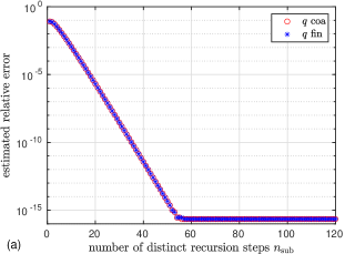
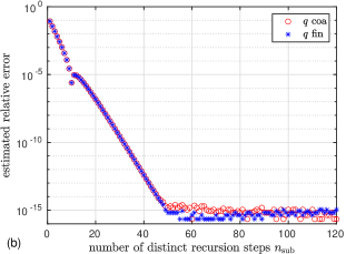
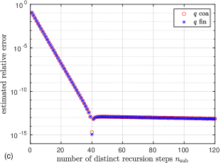
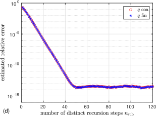
Figure 3: Convergence of $q$ with the number of distinct recursion levels $n_{\rm sub}$ in the example of Section 7.1.2. The singularity strengths $\alpha$ of (41) are taken as: (a) $\alpha=0.5$; (b) $\alpha=0.94$; (c) $\alpha=0.99$; (d) $\alpha=1+0.3{\rm i}$.

Figure 3 shows results obtained with $10$ quadrature panels on the coarse mesh on $\Gamma$, corresponding to $160$ discretization points on the coarse grid, and for various singularity strengths $\alpha$. For $\alpha<1$ and not too close to $1$, the results produced by our scheme are essentially fully accurate. Values of $q$ computed on the coarse grid ($q_{\rm coa}$) and on the fine grid ($q_{\rm fin}$) agree completely – indicating that the reconstruction procedure of Section 6 is stable.

Note, in Figure 3(d), that for $\alpha=1+0.3{\rm i}$, which corresponds to a singular right-hand side $f$ that is not even in $L^{1}$, the scheme loses only about two digits of accuracy. Note also that, thanks to the use of initializers, a number $n_{\rm sub}=60$ of distinct recursion steps is more than enough to make $q$ converge (to the achievable precision) for all values of $\alpha$ tested in Figure 3.

7.1.3 A one-corner example

We now consider an example where the corner opening angle in (39) is set to $\theta=\pi/2$. The contour $\Gamma$ then assumes the shape shown in Figure 1. The right-hand side of (1) is set to

$$f(r)=\frac{1}{\lvert r\rvert^{\alpha}}+\log{\lvert r\rvert}\,,\quad r\in\Gamma\,.$$ (44)

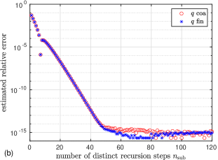
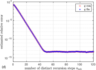
Figure 4: Convergence of $q$ with the number of distinct recursion levels $n_{\rm sub}$ in the example of Section 7.1.3. The singularity strengths $\alpha$ of (44) are taken as: (a) $\alpha=0.5$; (b) $\alpha=0.94$; (c) $\alpha=0.99$; (d) $\alpha=1+0.3{\rm i}$.

Figure 4, analogous to Figure 3, shows results obtained with $160$ discretization points on the coarse grid on $\Gamma$ and for various singularity strengths $\alpha$. In the absence of an analytical expression for $q$ we use, as a reference, the value of $q_{\rm coa}$ obtained with $n_{\rm sub}=500$. For example, with $\alpha=0.94$ this value is $q\approx 63.53529437281905$ and could be compared to the value $q\approx 63.53529437281894$, obtained with $29,\!088$ discretization points on the fine grid on $\Gamma$ using the $L^{1}$-norm-preserving Nyström discretization of Askham and Greengard [4, Section 4], which extends the $L^{2}$-inner-product-preserving discretization of Bremer [6, Section 2], in combination with compensated summation [22, 25]. Since the relative difference between these two reference values is on the order of our own error estimate in Figure 4(b), we believe that our error estimates are reliable also in Figure 4(c,d), where the norm-preserving discretization cannot be used due to memory constraints.

We add that the execution of our code is very rapid. The computing time, per data point, in Figure 4 varies with $n_{\rm sub}$ and also differs between $q_{\rm coa}$ and $q_{\rm fin}$, but it is much less than a second for all the data points shown.

7.2 The exterior Dirichlet Helmholtz problem

The exterior Dirichlet problem for the Helmholtz equation has been considered in [16, Section 18] in detail. Here we use this problem to illustrate that its solution $U(r)$ can be found accurately in the entire computational domain also when the right-hand side $f(r)$ is singular or nearly singular. The integral representation of $U(r)$ and the resulting boundary integral equation (a combined field integral equation) are identical to those in [16, Section 18]. The boundary $\Gamma$ is given by (39) with $\theta=\pi/2$. We consider two cases

1. Singular right-hand side
   The exact solution is

   $$U(r)=H_{0}^{(1)}(\omega|r|)$$ (45)

   with $f(r)$ being the restriction of $U(r)$ to $\Gamma$. Here $\omega$ is the wavenumber and $H_{0}^{(1)}$ is the first-kind Hankel function of order zero, that is, the field is generated by an acoustic monopole right at the corner.

2. Nearly singular right-hand side
   The exact solution is

   $$U(r)=H_{1}^{(1)}(\omega|r-r^{\prime}|)\frac{x-x^{\prime}}{|r-r^{\prime}|}\,,$$ (46)

   with $f(r)$ being the restriction of $U(r)$ to $\Gamma$, and $r^{\prime}=(10^{-10},0)$. That is, the field is generated by an acoustic dipole very close to the corner.

The integral equation [16, Eq. (68)] is solved with $\omega=10$ using the method in this paper, the singular point is taken as $\gamma=0$ both for (a) and for (b). For both cases, the coarse grid on $\Gamma$ has 56 panels, i.e., 896 discretization points; the number of refinement levels is set to $n_{\rm sub}=112$; and the number of GMRES iterations needed is 18. The field is evaluated using the scheme in [16, Section 20]. The solve phase takes about 4 seconds, while the field evaluation takes about 100 seconds, which can be accelerated via the fast multipole method [8] when necessary. A Cartesian grid of $200\times 200$ equispaced points is placed on the rectangle $[-0.1,1.1]\times[-0.53,0.53]$ and evaluations are carried out at those 27,760 grid points that are in the exterior domain. For case (a), 5,088 target points activate local panelwise evaluation for close panels; 920 target points close to the corner vertex require that the solution $\boldsymbol{\rho}_{\rm fin}$ on the fine grid is reconstructed using the backward recursion in Section 6. For case (b), the numbers are 6,364 and 1,326, respectively.

Figure 5 shows the absolute error in the numerical solution, demonstrating that our scheme achieves high accuracy in the entire computational domain for both singular and nearly singular right-hand sides. The small difference in achievable accuracy between (a) and (b) can chiefly be explained by that (b) has a stronger singularity in the right-hand side $f(r)$ than has (a) and is, thus, harder to resolve.

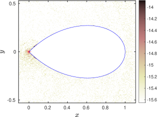
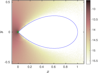
Figure 5: $\log_{10}$ of absolute error in the solution $U(r)$ to the exterior Dirichlet Helmholtz problem. The blue curve is the boundary $\Gamma$. Left: $U(r)$ is an acoustic monopole field with the source at $r^{\prime}=(0,0)$ shown as a red star. Right: $U(r)$ is an acoustic dipole field with the source at $r^{\prime}=(10^{-10},0)$ shown as a green star.

8 Application to the linearized BGKW equation for the Couette flow

Table 1: The velocity $u$ at $x=0.5$ at sample values of the Knudsen number $k$. Note that in [24], the interval is shifted from $[-0.5,0.5]$ to $[0,1]$. Thus, the velocity $u$ at $x=0.5$ is listed as $u$ at $x=1$ in Tables 1 and 2 in [24].

${k}$	${u(0.5)}$ in [24]	${u(0.5)}$ (current)	Error
$0.003$	$4.978\,915\,352\,789\,693\text{\cdot}{10}^{-01}$	$4.978\,915\,352\,789\,726\text{\cdot}{10}^{-01}$	$6.6\text{\cdot}{10}^{-15}$
$0.01$	$4.930\,697\,807\,742\,208\text{\cdot}{10}^{-01}$	$4.930\,697\,807\,742\,217\text{\cdot}{10}^{-01}$	$1.8\text{\cdot}{10}^{-15}$
$0.03$	$4.800\,058\,682\,766\,829\text{\cdot}{10}^{-01}$	$4.800\,058\,682\,766\,837\text{\cdot}{10}^{-01}$	$1.6\text{\cdot}{10}^{-15}$
$0.1$	$4.412\,246\,409\,722\,421\text{\cdot}{10}^{-01}$	$4.412\,246\,409\,722\,424\text{\cdot}{10}^{-01}$	$6.3\text{\cdot}{10}^{-16}$
$0.3$	$3.672\,125\,695\,500\,504\text{\cdot}{10}^{-01}$	$3.672\,125\,695\,500\,499\text{\cdot}{10}^{-01}$	$1.4\text{\cdot}{10}^{-15}$
$1.0$	$2.518\,613\,399\,894\,732\text{\cdot}{10}^{-01}$	$2.518\,613\,399\,894\,736\text{\cdot}{10}^{-01}$	$1.5\text{\cdot}{10}^{-15}$
$2.0$	$1.852\,462\,993\,740\,218\text{\cdot}{10}^{-01}$	$1.852\,462\,993\,740\,218\text{\cdot}{10}^{-01}$	$1.5\text{\cdot}{10}^{-16}$
$3.0$	$1.504\,282\,444\,992\,075\text{\cdot}{10}^{-01}$	$1.504\,282\,444\,992\,074\text{\cdot}{10}^{-01}$	$3.7\text{\cdot}{10}^{-16}$
$5.0$	$1.126\,351\,880\,294\,592\text{\cdot}{10}^{-01}$	$1.126\,351\,880\,294\,592\text{\cdot}{10}^{-01}$	$2.5\text{\cdot}{10}^{-16}$
$7.0$	$9.171\,689\,613\,521\,435\text{\cdot}{10}^{-02}$	$9.171\,689\,613\,521\,428\text{\cdot}{10}^{-02}$	$7.6\text{\cdot}{10}^{-16}$
$10.0$	$7.292\,211\,299\,328\,497\text{\cdot}{10}^{-02}$	$7.292\,211\,299\,328\,491\text{\cdot}{10}^{-02}$	$7.6\text{\cdot}{10}^{-16}$
$30.0$	$3.381\,357\,342\,231\,838\text{\cdot}{10}^{-02}$	$3.381\,357\,342\,231\,840\text{\cdot}{10}^{-02}$	$6.2\text{\cdot}{10}^{-16}$
$100.0$	$1.343\,072\,948\,081\,877\text{\cdot}{10}^{-02}$	$1.343\,072\,948\,081\,874\text{\cdot}{10}^{-02}$	$1.9\text{\cdot}{10}^{-15}$

In this section, we revisit the integral equation that is derived from the linearized BGKW equation for the steady Couette flow [7, 24, 27]

$$u(x)-\frac{1}{k\sqrt{\pi}}\int_{-0.5}^{0.5}J_{-1}\left(\frac{|x-y|}{k}\right)u(y)\,{\rm d}y=f(x)\,,\quad x\in[-0.5,0.5]\,,$$ (47a)

$$f(x)=\frac{1}{2\sqrt{\pi}}\left[J_{0}\left(\frac{0.5-x}{k}\right)-J_{0}\left(\frac{0.5+x}{k}\right)\right],$$ (47b)

where the parameter $k$ is the Knudsen number and $J_{n}$ is the $n$th order Abramowitz function defined by

$$J_{n}(x)=\int_{0}^{\infty}t^{n}e^{-t^{2}-x/t}\,{\rm d}t\,,\quad n\geq-1\,.$$ (48)

See, for example, [13] and references therein for the properties of Abramowitz functions and an accurate numerical scheme for their evaluation. The BGKW equation has been studied in [24], where it is shown that the solution of (47a) contains singular terms $(x\ln x)^{n}$ for $n\in\mathbb{N}:=\{1,\,2,\,\ldots\}$ at the endpoints. It is known that the kernel function $J_{-1}(x)$ has both absolute value and logarithmic singularities at $x=0$, and that the right-hand-side function (47b) has $x\ln x$ singularity at the endpoints. Benchmark calculations have been carried out in [24], using dyadic refinement towards the endpoints to treat the singularities of the solution and the right-hand-side function, and generalized Gaussian quadrature [28] to treat the kernel singularities.

Table 2: The stress $P_{xy}$ at sample values of the Knudsen number $k$.

${k}$	${P_{xy}}$ in [24]	${P_{xy}}$ (current)	Error
$0.003$	$-1.490\,909\,702\,131\,201\text{\cdot}{10}^{-03}$	$-1.490\,909\,702\,131\,188\text{\cdot}{10}^{-03}$	$8.7\text{\cdot}{10}^{-15}$
$0.01$	$-4.900\,405\,009\,657\,547\text{\cdot}{10}^{-03}$	$-4.900\,405\,009\,657\,524\text{\cdot}{10}^{-03}$	$4.8\text{\cdot}{10}^{-15}$
$0.03$	$-1.413\,798\,601\,526\,842\text{\cdot}{10}^{-02}$	$-1.413\,798\,601\,526\,841\text{\cdot}{10}^{-02}$	$4.9\text{\cdot}{10}^{-16}$
$0.1$	$-4.155\,607\,782\,558\,620\text{\cdot}{10}^{-02}$	$-4.155\,607\,782\,558\,619\text{\cdot}{10}^{-02}$	$3.3\text{\cdot}{10}^{-16}$
$0.3$	$-9.344\,983\,511\,356\,682\text{\cdot}{10}^{-02}$	$-9.344\,983\,511\,356\,685\text{\cdot}{10}^{-02}$	$3.0\text{\cdot}{10}^{-16}$
$1.0$	$-1.694\,625\,753\,368\,226\text{\cdot}{10}^{-01}$	$-1.694\,625\,753\,368\,225\text{\cdot}{10}^{-01}$	$3.3\text{\cdot}{10}^{-16}$
$2.0$	$-2.083\,322\,536\,749\,375\text{\cdot}{10}^{-01}$	$-2.083\,322\,536\,749\,375\text{\cdot}{10}^{-01}$	$0.0\text{\cdot}{10}^{00}$
$3.0$	$-2.266\,437\,497\,658\,084\text{\cdot}{10}^{-01}$	$-2.266\,437\,497\,658\,084\text{\cdot}{10}^{-01}$	$0.0\text{\cdot}{10}^{00}$
$5.0$	$-2.446\,632\,678\,455\,994\text{\cdot}{10}^{-01}$	$-2.446\,632\,678\,455\,994\text{\cdot}{10}^{-01}$	$0.0\text{\cdot}{10}^{00}$
$7.0$	$-2.536\,943\,539\,674\,479\text{\cdot}{10}^{-01}$	$-2.536\,943\,539\,674\,479\text{\cdot}{10}^{-01}$	$0.0\text{\cdot}{10}^{00}$
$10.0$	$-2.611\,624\,603\,488\,405\text{\cdot}{10}^{-01}$	$-2.611\,624\,603\,488\,405\text{\cdot}{10}^{-01}$	$0.0\text{\cdot}{10}^{00}$
$30.0$	$-2.743\,853\,873\,277\,227\text{\cdot}{10}^{-01}$	$-2.743\,853\,873\,277\,228\text{\cdot}{10}^{-01}$	$2.0\text{\cdot}{10}^{-16}$
$100.0$	$-2.796\,682\,147\,138\,912\text{\cdot}{10}^{-01}$	$-2.796\,682\,147\,138\,912\text{\cdot}{10}^{-01}$	$2.0\text{\cdot}{10}^{-16}$

Table 3: The half-channel mass flow rate $Q$ at sample values of the Knudsen number $k$.

${k}$	${Q}$ in [24]	${Q}$ (current)	Error
$0.003$	$1.242\,445\,655\,299\,172\text{\cdot}{10}^{-01}$	$1.242\,445\,655\,299\,167\text{\cdot}{10}^{-01}$	$4.4\text{\cdot}{10}^{-15}$
$0.01$	$1.225\,330\,275\,292\,623\text{\cdot}{10}^{-01}$	$1.225\,330\,275\,292\,621\text{\cdot}{10}^{-01}$	$1.8\text{\cdot}{10}^{-15}$
$0.03$	$1.180\,147\,037\,188\,893\text{\cdot}{10}^{-01}$	$1.180\,147\,037\,188\,893\text{\cdot}{10}^{-01}$	$1.2\text{\cdot}{10}^{-16}$
$0.1$	$1.057\,028\,408\,172\,292\text{\cdot}{10}^{-01}$	$1.057\,028\,408\,172\,292\text{\cdot}{10}^{-01}$	$2.6\text{\cdot}{10}^{-16}$
$0.3$	$8.560\,111\,699\,820\,618\text{\cdot}{10}^{-02}$	$8.560\,111\,699\,820\,613\text{\cdot}{10}^{-02}$	$4.9\text{\cdot}{10}^{-16}$
$1.0$	$5.804\,708\,735\,555\,459\text{\cdot}{10}^{-02}$	$5.804\,708\,735\,555\,460\text{\cdot}{10}^{-02}$	$2.4\text{\cdot}{10}^{-16}$
$2.0$	$4.281\,659\,776\,113\,917\text{\cdot}{10}^{-02}$	$4.281\,659\,776\,113\,918\text{\cdot}{10}^{-02}$	$1.6\text{\cdot}{10}^{-16}$
$3.0$	$3.489\,298\,506\,190\,833\text{\cdot}{10}^{-02}$	$3.489\,298\,506\,190\,833\text{\cdot}{10}^{-02}$	$2.0\text{\cdot}{10}^{-16}$
$5.0$	$2.627\,042\,060\,967\,383\text{\cdot}{10}^{-02}$	$2.627\,042\,060\,967\,383\text{\cdot}{10}^{-02}$	$1.3\text{\cdot}{10}^{-16}$
$7.0$	$2.147\,460\,412\,330\,841\text{\cdot}{10}^{-02}$	$2.147\,460\,412\,330\,841\text{\cdot}{10}^{-02}$	$1.6\text{\cdot}{10}^{-16}$
$10.0$	$1.714\,449\,048\,590\,649\text{\cdot}{10}^{-02}$	$1.714\,449\,048\,590\,649\text{\cdot}{10}^{-02}$	$2.0\text{\cdot}{10}^{-16}$
$30.0$	$8.043\,009\,085\,700\,258\text{\cdot}{10}^{-03}$	$8.043\,009\,085\,700\,263\text{\cdot}{10}^{-03}$	$6.5\text{\cdot}{10}^{-16}$
$100.0$	$3.226\,757\,181\,742\,400\text{\cdot}{10}^{-03}$	$3.226\,757\,181\,742\,397\text{\cdot}{10}^{-03}$	$9.4\text{\cdot}{10}^{-16}$

We have implemented the method of this paper, based on (10), to solve (47a). We note that both endpoints are singular points and there is only one side to each singular point, since we are dealing with an open arc instead of a closed contour. This leads to straightforward modifications in the method and its implementation. Some implementation details are as follows. First, the kernel-split quadrature is applied to treat the kernel singularity: the correction to the logarithmic singularity was done in [15]; the correction on diagonal blocks for the absolute value singularity can be derived easily in an identical manner; the splitting of the kernel into various parts is done using either the series expansion of the Abramowitz function [1] or the Chebyshev expansion for each part as in [29]. When the Knudsen number is low, the kernel is sharply peaked at the origin. A modified version of the upsampling scheme in [2] is used to resolve the sharp peak of the kernel accurately and efficiently so that the coarse panels only need to resolve the features of the solution. Here the modification is that the exact centering in [2] is not enforced for local adaptive panels for each target. Instead, the so-called level-restricted property [11], i.e., sizes of adjacent panels can differ at most by a factor of 2, is used to ensure the accuracy in the calculation of the integrals. We remark that the cost of the upsampling scheme is $O(\log(1/k))$ as $k\rightarrow 0$, the same as that in [2].

Second, it is observed numerically that the condition number of the integral equation (47a) increases as $k$ decreases, reaching about $2\cdot 10^{4}$ for $k=0.003$. On the other hand, the solution $u(x)$ approaches the asymptotic solution $u_{\rm asym}(x)=x$ as $k\rightarrow 0$. Thus, in order to reduce the effect of the ill-conditioning of the integral equation for small values of $k$, we write $u(x)=w(x)+x$ and solve the following equation for $w(x)$ instead when $k\leq 0.3$:

$$w(x)-\frac{1}{k\sqrt{\pi}}\int_{-0.5}^{0.5}J_{-1}\left(\frac{|x-y|}{k}\right)w(y)\,{\rm d}y=h(x)\,,\quad x\in[-0.5,0.5]\,,$$ (49a)

$$h(x)=-\frac{k}{\sqrt{\pi}}\left[J_{1}\left(\frac{0.5-x}{k}\right)-J_{1}\left(\frac{0.5+x}{k}\right)\right].$$ (49b)

Since $w(x)$ is a small perturbation when $k$ is small, the inaccuracy in the calculation of $w(x)$ has almost no effect on the overall accuracy of $u(x)$. This allows us to achieve the machine precision for all physical quantities of interest for a much wider range of the Knudsen number $k$ than reported in [24].

We have repeated the calculations in [24] using the current method. For all values of $k$, the computational domain $[-0.5,0.5]$ is divided into four coarse panels; $n_{\rm sub}$ is set to $41$; and the GMRES stopping criterion is set to machine epsilon. Tables 1–3 list the values of the velocity $u$ at $x=0.5$, the stress $P_{xy}$ [24, Eq. (43)] and the half-channel mass flow rate $Q$ [24, Eq. (42)] at sample values of the Knudsen number $k$, where the second column contains the values in [24], the third column contains the values using the current method, and the last column shows the relative difference between these values. Here $u(0.5)$ is obtained via the backward recursion in Section 6, $P_{xy}$ and $Q$ are calculated using the velocity on the coarse grid with the kernel-split quadrature applied to treat the logarithmic singularity of $J_{0}(x)$ at $x=0$ in $P_{xy}$. It is clear that the numerical results agree with those in [24] to machine precision for all sample values of $k$.

The current method is much more efficient as compared with the one used in [24]. For $k=0.003$, the computation takes about $0.05$ second of CPU time; and for $k=10$, the computational time becomes unmeasurable with Matlab’s cputime command for a single run, i.e., less than $0.01$ second. In [24], the timing results are $62.8$ and $23.9$ seconds, respectively. The RCIP method eliminates the dyadic refinement towards the endpoints in the solve phase, and the upsampling scheme allows us to use such coarse panels that they only need to capture the features of the solution. The combination of these two techniques enables us to use the optimal number of discretization points for constructing the system matrix. The full machine precision accuracy of the current method completely removes the need of using quadruple precision arithmetic. Finally, the preconditioner ${\bf R}$ also reduces the number of GMRES iterations. Indeed, the number of GMRES iterations required is at most $6$ for all sample values of $k$, whereas $430$ was reported in [24] for $k=0.003$. All of this results in a significant reduction in the computational cost, i.e., a speedup of at least a factor of $1000$.

9 Concluding remarks

Finding efficient solvers for SKIEs on non-smooth boundaries is a field with substantial recent activity. However, almost all existing methods only work well for smooth right-hand sides and may also involve a fair amount of operator-specific analysis and precomputed quantities. In contrast, the method constructed in this paper for singular and nearly singular right-hand sides computes all intermediary quantities needed on-the-fly and only involves a bare minimum of analysis.

The extension of the current method to multiple right-hand sides can be carried out easily. The compressed inverse ${\bf R}$ is independent on $f$ and needs only to be computed once, while the compressed inverse ${\bf R}_{f}$ depends on $f$ and needs to be computed afresh for each new $f$. The setup cost of ${\bf R}_{f}$ for each additional $f$ can, furthermore, be reduced since several of the matrices entering into the forward recursion for ${\bf R}_{f}$ are independent of $f$ and can be stored after they have been computed on-the-fly. A similar situation holds in the backward recursions for $\rho$ on the fine grid – should that quantity be needed.

In a certain sense, the work completes the RCIP method in two dimensions since the splitting into a smooth part and a local singular part is carried out on both sides of the integral equation. The RCIP method can be generalized to three dimensions. In [20], the RCIP method was extended to solve a boundary integral equation on the surface of a cube. In [18], it was extended to solve boundary integral equations on axially symmetric surfaces. In a recent talk [12], an RCIP-type scheme for discretizing corner and edge singularities in three dimensions was discussed. For general surfaces in three dimensions, the extension of the RCIP is more or less straightforward when the geometry admits a local hierarchical discretization near the corner and edge singularities; and the extension of the work in this paper should follow subsequently.

Appendix A Derivation of the forward recursion formula (20) for ${\bf R}_{f}$

First, we prove the following lemma.

Lemma 1.

Suppose that ${\bf A}$ is an invertible $m\times m$ matrix, ${\bf B}$ is an $n\times n$ matrix, ${\bf U}$ is an $n\times m$ matrix, and ${\bf V}$ is an $m\times n$ matrix with $m\geq n$. Suppose further that ${\bf U}{\bf A}^{-1}{\bf V}$ and ${\bf A}+{\bf V}{\bf B}{\bf U}$ are both invertible. Then

$${\bf U}({\bf A}+{\bf V}{\bf B}{\bf U})^{-1}{\bf V}=\left(({\bf U}{\bf A}^{-1}{\bf V})^{-1}+{\bf B}\right)^{-1},$$ (50)

$${\bf U}({\bf A}+{\bf V}{\bf B}{\bf U})^{-1}=\left(({\bf U}{\bf A}^{-1}{\bf V})^{-1}+{\bf B}\right)^{-1}({\bf U}{\bf A}^{-1}{\bf V})^{-1}{\bf U}{\bf A}^{-1}.$$ (51)

Proof.

Introduce a complex parameter $\lambda$ and consider $({\bf A}+\lambda{\bf V}{\bf B}{\bf U})^{-1}$. When $\lambda$ is sufficiently small, the following Taylor expansion is valid

$$({\bf A}+\lambda{\bf V}{\bf B}{\bf U})^{-1}={\bf A}^{-1}-\lambda{\bf A}^{-1}{\bf V}{\bf B}{\bf U}{\bf A}^{-1}+\lambda^{2}{\bf A}^{-1}{\bf V}{\bf B}{\bf U}{\bf A}^{-1}{\bf V}{\bf B}{\bf U}{\bf A}^{-1}-\ldots,$$ (52)

Mutiplying both sides of (52) with ${\bf U}$ from the left and with ${\bf V}$ from the right and regrouping, we obtain

$${\bf U}({\bf A}+\lambda{\bf V}{\bf B}{\bf U})^{-1}{\bf V} ={\bf U}{\bf A}^{-1}{\bf V}-\lambda\left({\bf U}{\bf A}^{-1}{\bf V}\right){\bf B}\left({\bf U}{\bf A}^{-1}{\bf V}\right)$$ (53)

$$+\lambda^{2}\left({\bf U}{\bf A}^{-1}{\bf V}\right){\bf B}\left({\bf U}{\bf A}^{-1}{\bf V}\right){\bf B}\left({\bf U}{\bf A}^{-1}{\bf V}\right)-\ldots$$

$$=\left(\left({\bf U}{\bf A}^{-1}{\bf V}\right)^{-1}+\lambda{\bf B}\right)^{-1},$$

where the second equality follows from the application of the Taylor expansion in the reverse order. By the cofactor formula of the matrix inverse and the so-called big formula for the matrix determinant [34], both sides of (53) are rational functions of $\lambda$. Since these two rational functions are equal in a small neighborhood of the origin in the complex plane, they must be equal everywhere in the whole complex plane by analytic continuation [3]. Setting $\lambda=1$ in (53), we establish (51) and the invertibility of $({\bf U}{\bf A}^{-1}{\bf V})^{-1}+{\bf B}$ simultaneously. (51) can be proved in an almost identical manner. ∎

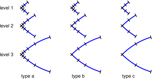
Figure 6: Meshes of type a, type b, and type c at different levels. The type a mesh contains $4+2i$ dyadic fine panels at level $i$. The type b mesh always contains six panels, and the type c mesh always contains four panels. At level $1$, the type a mesh is identical to the type b mesh. At level $n_{\rm sub}$, the type c mesh contains four coarse panels on $\Gamma^{\star}$ in Figure 1.

We now recall the definition of ${\bf R}_{f}$ in (16)

$${\bf R}_{f}={\bf P}_{W}^{\rm T}\left({\bf I}_{\rm fin}+{\bf K}_{\rm fin}^{\star}\right)^{-1}{\bf P}_{f}\,,$$ (54)

where ${\bf K}_{\rm fin}^{\star}$ is the system matrix built on a fine mesh that is obtained via $n_{\rm sub}$ level of dyadic refinement of the four coarsest panels (with two panels on each side) near the singular point. Let $n_{\rm gl}$ be the number of Gauss-Legendre nodes on each panel. Then the total number of discretization points on the fine mesh is $n_{\rm gl}(4+2n_{\rm sub})$. Clearly, direct application of $\eqref{rfdef}$ is very expensive, inaccurate, and unrobust. Instead, the forward recursion is used to compute ${\bf R}_{f}$. The forward recursion starts from the finest six panels around the singular point at level $i=1$, adds one panel on each side as the level goes up, and reaches the full fine mesh at level $i=n_{\rm sub}$. See Figure 6 for an illustration of three different types of meshes at different levels, where the type a mesh is needed only in the derivation of the forward recursion. The actual recursion formula involves only type b and type c meshes. To be more precise, at any step in the forward recursion, one only needs to build a system matrix of size $6n_{\rm gl}\times 6n_{\rm gl}$, i.e., on the six panels of a type b mesh, and the type c mesh is used only implicitly in the construction of the prolongation matrix ${\bf P}$ and its weighted version ${\bf P}_{W}$. Similar to [16, Eq. (D.1)], we define

$${\bf R}_{fi}\coloneqq{\bf P}_{Wi{\rm ac}}^{T}({\bf I}_{i{\rm a}}+{\bf K}_{i{\rm a}})^{-1}{\bf P}_{fi{\rm ac}},\qquad i=1,\cdots,n_{\rm sub}.$$ (55)

By the action of ${\bf P}_{fi{\rm ac}}$ and ${\bf P}_{Wi{\rm ac}}^{T}$, ${\bf R}_{fi}$ is always a matrix of size $4n_{\rm gl}\times 4n_{\rm gl}$ at any level $i$. A derivation similar to that of [16, Eq. (D.6)] leads to

$${\bf R}_{fi}={\bf P}_{W{\rm bc}}^{T}{\bf P}_{Wi{\rm ab}}^{T}({\bf I}_{i{\rm a}}+\mathbb{F}\{{\bf K}_{(i-1){\rm a}}\}+{\bf P}_{i{\rm ab}}{\bf K}_{i{\rm b}}^{\circ}{\bf P}_{Wi{\rm ab}}^{T})^{-1}{\bf P}_{fi{\rm ab}}{\bf P}_{fi{\rm bc}},$$ (56)

where we have assumed that the low-rank property

$${\bf K}_{i{\rm a}}^{\circ}={\bf P}_{i{\rm ab}}{\bf K}_{i{\rm b}}^{\circ}{\bf P}_{Wi{\rm ab}}^{T}$$ (57)

holds to machine precision, as in [16, Eq. (D.3)]. Since the type a mesh differs from the type b mesh only on the two panels (i.e., $\Gamma_{i{\rm b}}^{\star\star}$) closest to the singular point in the type b mesh, the only diagonal blocks in ${\bf P}_{i{\rm ab}}$ and ${\bf P}_{Wi{\rm ab}}$ that are not identity matrices are ${\bf P}_{i{\rm ab}}({\rm I}_{i{\rm a}}^{\star\star},{\rm I}_{i{\rm b}}^{\star\star})$ and ${\bf P}_{Wi{\rm ab}}({\rm I}_{i{\rm a}}^{\star\star},{\rm I}_{i{\rm b}}^{\star\star})$, respectively. Here ${\rm I}_{i{\rm a}}^{\star\star}$ and ${\rm I}_{i{\rm b}}^{\star\star}$ contain indices corresponding to discretization points in $\Gamma_{i{\rm b}}^{\star\star}$ on type a and type b meshes, respectively. Now it is straightforward to verify that (57) is equivalent to

$${\bf K}_{i{\rm a}}({\rm I}_{i{\rm a}}^{\star\star},{\rm I}_{i{\rm b}}^{\circ}) ={\bf P}_{i{\rm ab}}({\rm I}_{i{\rm a}}^{\star\star},{\rm I}_{i{\rm b}}^{\star\star}){\bf K}_{i{\rm b}}({\rm I}_{i{\rm b}}^{\star\star},{\rm I}_{i{\rm b}}^{\circ})\,,$$ (58)

$${\bf K}_{i{\rm a}}({\rm I}_{i{\rm b}}^{\circ},{\rm I}_{i{\rm a}}^{\star\star}) ={\bf K}_{i{\rm b}}({\rm I}_{i{\rm b}}^{\circ},{\rm I}_{i{\rm b}}^{\star\star}){\bf P}_{Wi{\rm ab}}^{T}({\rm I}_{i{\rm b}}^{\star\star},{\rm I}_{i{\rm a}}^{\star\star})\,,$$

where ${\rm I}_{i{\rm b}}^{\circ}$ contains indices corresponding to discretization points on $\Gamma_{i{\rm b}}^{\circ}$, that is, on the two outermost panels from $\gamma$. Since $\Gamma_{i{\rm b}}^{\star\star}$ is always well-separated from $\Gamma_{i{\rm b}}^{\circ}$ for any level $i$, (58) is equivalent to stating that the kernel function $K(r,r^{\prime})$ is smooth when $r\in\Gamma_{i{\rm b}}^{\star\star}$ and $r^{\prime}\in\Gamma_{i{\rm b}}^{\circ}$, or vice versa, and thus the interaction between $\Gamma_{i{\rm b}}^{\star\star}$ and $\Gamma_{i{\rm b}}^{\circ}$ can be discretized to machine precision with $n_{\rm gl}$ points on each panel in $\Gamma_{i{\rm b}}^{\star\star}$ provided that $n_{\rm gl}$ is not too small. This holds for all kernels we have encountered in practice, including, say, highly oscillatory ones, if the coarse mesh is chosen in such a way that the oscillations of the kernel are well-resolved. We emphasize that this is a property of the kernel function $K(r,r^{\prime})$ and the type a and b meshes. It has nothing to do with the singularity of the right-hand side $f$.

Applying (51) to part of the right-hand side of (56), we obtain

$${\bf P}_{Wi{\rm ab}}^{T}({\bf I}_{i{\rm a}}+\mathbb{F}\{{\bf K}_{(i-1){\rm a}}\}+{\bf P}_{i{\rm ab}}{\bf K}_{i{\rm b}}^{\circ}{\bf P}_{Wi{\rm ab}}^{T})^{-1}=$$ (59)

$$\left[\left({\bf P}_{Wi{\rm ab}}^{T}({\bf I}_{i{\rm a}}+\mathbb{F}\{{\bf K}_{(i-1){\rm a}}\})^{-1}{\bf P}_{i{\rm ab}}\right)^{-1}+{\bf K}_{i{\rm b}}^{\circ}\right]^{-1}$$

$$\cdot\left({\bf P}_{Wi{\rm ab}}^{T}({\bf I}_{i{\rm a}}+\mathbb{F}\{{\bf K}_{(i-1){\rm a}}\})^{-1}{\bf P}_{i{\rm ab}}\right)^{-1}{\bf P}_{Wi{\rm ab}}^{T}({\bf I}_{i{\rm a}}+\mathbb{F}\{{\bf K}_{(i-1){\rm a}}\})^{-1}.$$

Recall that [16, Eq. (D.10)] states that

$$\mathbb{F}\{{\bf R}_{i-1}\}+{\bf I}_{\rm b}^{\circ}={\bf P}_{Wi{\rm ab}}^{T}({\bf I}_{i{\rm a}}+\mathbb{F}\{{\bf K}_{(i-1){\rm a}}\})^{-1}{\bf P}_{i{\rm ab}}.$$ (60)

Figure 7: Nonzero patterns of $\mathbb{F}\{{\bf R}_{i-1}^{-1}\}$ and $\mathbb{F}\{{\bf R}_{f(i-1)}\}$ (left), ${\bf K}_{i{\rm b}}^{\circ}$ (center), and ${\bf I}_{\rm b}^{\circ}$ (right). Note that the patterns depend on the fact that when constructing the system matrix in the forward recursion, the sources and targets are arranged in the order from the top panel to the bottom panel on a type b mesh, see Figure 6.

We observe that $\mathbb{F}\{{\bf R}_{i-1}\}$ places ${\bf R}_{i-1}$ in the center $4n_{\rm gl}\times 4n_{\rm gl}$ block with zero padding in a $6n_{\rm gl}\times 6n_{\rm gl}$ matrix, and the nonzero blocks of ${\bf I}_{\rm b}^{\circ}$ are the identity matrix of size $n_{\rm gl}$ in the top and bottom diagonal blocks (Figure 7). Thus,

$$\mathbb{F}\{{\bf R}_{i-1}^{-1}\}+{\bf I}_{\rm b}^{\circ} =\left(\mathbb{F}\{{\bf R}_{i-1}\}+{\bf I}_{\rm b}^{\circ}\right)^{-1}$$ (61)

$$=\left({\bf P}_{Wi{\rm ab}}^{T}({\bf I}_{i{\rm a}}+\mathbb{F}\{{\bf K}_{(i-1){\rm a}}\})^{-1}{\bf P}_{i{\rm ab}}\right)^{-1}.$$

Similarly,

$$\mathbb{F}\{{\bf R}_{f(i-1)}\} =\mathbb{F}\{{\bf P}_{W(i-1){\rm ac}}^{T}({\bf I}_{(i-1){\rm a}}+{\bf K}_{(i-1){\rm a}})^{-1}{\bf P}_{f(i-1){\rm ac}}\}$$ (62)

$$={\bf P}_{Wi{\rm ab}}^{T}({\bf I}_{i{\rm a}}+\mathbb{F}\{{\bf K}_{(i-1){\rm a}}\})^{-1}{\bf P}_{fi{\rm ab}}-{\bf I}_{\rm b}^{\circ},$$

where the second equality uses $\left({\bf P}_{Wi{\rm ab}}^{T}{\bf P}_{fi{\rm ab}}\right)^{\circ}={\bf I}_{\rm b}^{\circ}$. Combining (56), (59)–(62), we obtain

$${\bf R}_{fi}={\bf P}_{W{\rm bc}}^{T}\left(\mathbb{F}\{{\bf R}_{i-1}^{-1}\}+{\bf I}_{\rm b}^{\circ}+{\bf K}_{i{\rm b}}^{\circ}\right)^{-1}\left(\mathbb{F}\{{\bf R}_{i-1}^{-1}\}+{\bf I}_{\rm b}^{\circ}\right)\left(\mathbb{F}\{{\bf R}_{f(i-1)}\}+{\bf I}_{\rm b}^{\circ}\right){\bf P}_{fi{\rm bc}}.$$ (63)

Finally, we arrive at (20) by observing that

$$\left(\mathbb{F}\{{\bf R}_{i-1}^{-1}\}+{\bf I}_{\rm b}^{\circ}\right)\left(\mathbb{F}\{{\bf R}_{f(i-1)}\}+{\bf I}_{\rm b}^{\circ}\right)=\mathbb{F}\{{\bf R}_{i-1}^{-1}{\bf R}_{f(i-1)}\}+{\bf I}_{\rm b}^{\circ},$$ (64)

due to the nonzero patterns of the involved matrices shown in Figure 7.

Appendix B A synopsis of the RCIP demo codes

On the website http://www.maths.lth.se/na/staff/helsing/Tutor/, maintained by the first author, a set of Matlab demo codes are posted so that researchers who are interested in the RCIP method can download and run them and gain first-hand experience about the method’s efficiency, accuracy, and robustness for a few chosen problems. The codes are written so that they can easily be modified to solve other problems. The reader is expected to read the tutorial [16] in tandem with looking at the codes. Many demo codes use the one-corner contour $\Gamma$ in Figure 1, which is parameterized by $s\in[0,1]$ with $s=0$ corresponding to the corner at the origin, and going back to the corner again in the counterclockwise direction as $s$ increases to $s=1$. Most demo codes consist of the following building blocks or functions:

• Boundary discretization functions. These include the discretization in parameter space using panel division and functions returning $z(s)$, $z^{\prime}(s)$, $z^{\prime\prime}(s)$ in complex form for a given parameter value $s$, e.g., zfunc, zpfunc, zppfunc, zinit, panelinit.

• Integral operator discretization functions. These include splitting of the kernel into various parts – smooth part, logarithmically singular part, Cauchy singular part, hypersingular part, etc., corrections for singular and nearly singular integrals (explicit kernel-split quadrature), e.g., LogCinit, WfrakLinit, wLCinit, StargClose, KtargClose.

• System matrix construction functions such as MAinit, MRinit, Soperinit, Koperinit.

• Functions for the forward recursion formula for computing the nontrivial block of ${\bf R}$. These include zlocinit, Rcomp, SchurBana.

• Other utility functions such as myGMRES, Tinit16, Winit16 that are self-explanatory.

We now provide some comments on the forward recursion functions. In the discussions below, $n_{\rm gl}=16$, as in most demo codes. The function zlocinit returns a discretization on the type b mesh at level $i$, where the points are always arranged in the order from the top panel to the bottom panel. Another important feature is that in zlocinit, the singular points $\gamma_{j}$ is translated to the origin to reduce the effect of round-off error. See Figure 9 for detailed comments on zlocinit.

Recall from (18) that the forward recursion formula for ${\bf R}$ is

$${\bf R}_{i}={\bf P}^{T}_{W\rm{bc}}\left(\mathbb{F}\{{\bf R}_{i-1}^{-1}\}+{\bf I}_{\rm b}^{\circ}+{\bf K}_{i{\rm b}}^{\circ}\right)^{-1}{\bf P}_{\rm{bc}}\,,\quad i=1,\ldots,n_{\rm sub}\,.$$ (65)

Let ${\bf M}_{i}\coloneqq{\bf I}_{\rm b}+{\bf K}_{i{\rm b}}$ and ${\bf M}_{i}^{\circ}\coloneqq{\bf I}_{\rm b}^{\circ}+{\bf K}_{i{\rm b}}^{\circ}$. Then Figure 7 shows that there is no overlap in nonzero entries of ${\bf M}_{i}^{\circ}$ and ${\bf R}_{i-1}$. Direct implementation of (65) is shown in Algorithm 1.

Algorithm 1 Forward recursion via direct implementation of (65).

1:for $i=1,\ldots,n_{\rm sub}$ do

2:     Obtain 96 discretization points on the type b mesh at level $i$.

3:     Construct $96\times 96$ system matrix ${\bf M}_{i}$ at level $i$.

4:     if $i==1$ then

5:         ${\bf R}_{0}={\bf M}_{1}^{\star-1}$. That is, ${\bf R}_{0}$ is the inverse of the center $64\times 64$

6:            block of ${\bf M}_{1}$.

7:     end if

8:     Compute ${\bf R}_{i-1}^{-1}$.

9:     Replace the center $64\times 64$ block of ${\bf M}_{i}$ with ${\bf R}_{i-1}^{-1}$ to obtain $\widetilde{{\bf M}}_{i}$.

10:     Compute $\widetilde{{\bf M}}_{i}^{-1}$.

11:     Compress $\widetilde{{\bf M}}_{i}^{-1}$ to obtain ${\bf R}_{i}$. To be more precise, ${\bf R}_{i}={\bf P}^{T}_{W\rm{bc}}\widetilde{{\bf M}}_{i}^{-1}{\bf P}_{\rm{bc}}$.

12:end for

13:Return the nontrivial $64\times 64$ block of ${\bf R}$, i.e., ${\bf R}_{n_{\rm sub}}$.

Algorithm 1 needs to invert two matrices, i.e., ${\bf R}_{i-1}$ of size $64\times 64$ and $\widetilde{{\bf M}}_{i}$ of size $96\times 96$. This may lead to loss of accuracy and even instability when ${\bf R}_{i-1}$ is ill-conditioned. As pointed out in Section 4.3, the algorithm can be improved via the block matrix inversion formula that avoids explicit inversion of ${\bf R}_{i-1}$. Indeed, after column and row permutations, we obtain the following block structure (Figure 8)

$$\mathbb{F}\{{\bf R}_{i-1}^{-1}\}+{\bf I}_{\rm b}^{\circ}+{\bf K}_{i{\rm b}}^{\circ}\longrightarrow\left[\begin{array}[]{c c}{\bf A}^{-1}&{\bf U}\\ {\bf V}&{\bf D}\end{array}\right]\,.$$ (66)

Figure 8: Column/row permutation converting $\mathbb{F}\{{\bf R}_{i-1}^{-1}\}+{\bf I}_{\rm b}^{\circ}+{\bf K}_{i{\rm b}}^{\circ}$ into a $2\times 2$ block matrix. Blue block is ${\bf R}_{i-1}^{-1}$ and red block is ${\bf I}_{\rm b}^{\circ}+{\bf K}_{i{\rm b}}^{\circ}$. Left: the original matrix $\mathbb{F}\{{\bf R}_{i-1}^{-1}\}+{\bf I}_{\rm b}^{\circ}+{\bf K}_{i{\rm b}}^{\circ}$. Right: the matrix after column/row permutation.

However, there is no need to carry out column/row permutation explicitly. Matlab’s column/row indexing conveniently achieves this purpose without actual permutation. To be more precise, ${\bf A}={\bf R}_{i-1}$ is a $64\times 64$ block, ${\bf D}={\bf M}_{i}^{\circ}({\tt circL},{\tt circL})$ is a $32\times 32$ block, ${\bf U}={\bf M}_{i}^{\circ}({\tt starL},{\tt circL})$ is a $64\times 32$ block, and ${\bf V}={\bf M}_{i}^{\circ}({\tt circL},{\tt starL})$ is a $32\times 64$ block, where circL=[1:16  81:96] and starL=17:80. And [16, Eq. (31)] follows from the following block matrix inversion formula

$$\begin{bmatrix}{\bf A}^{-1}&{\bf U}\\ {\bf V}&{\bf D}\end{bmatrix}^{-1}=\begin{bmatrix}{\bf A}+{\bf A}{\bf U}({\bf D}-{\bf V}{\bf A}{\bf U})^{-1}{\bf V}{\bf A}&-{\bf A}{\bf U}({\bf D}-{\bf V}{\bf A}{\bf U})^{-1}\\ -({\bf D}-{\bf V}{\bf A}{\bf U})^{-1}{\bf V}{\bf A}&({\bf D}-{\bf V}{\bf A}{\bf U})^{-1}\end{bmatrix},$$ (67)

which can be verified via direct matrix multiplication. Thus, in order to achieve better efficiency and stability, Algorithm 1 is replaced by function Rcomp (Figure 10) that contains the main loop for the forward recursion, and function SchurBana (Figure 11) that replaces steps 8–11 in Algorithm 1 by [16, Eq. (31)]. We note that one only needs to invert a $32\times 32$ matrix in function SchurBana.

⬇

function [z,zp,zpp,nz,w,wzp]=zlocinit(theta,T,W,nsub,i,npan)

% This function returns to the user the discretization of

% the type b mesh at the ith level

%

% Input parameters:

% theta - the parameter for the one-corner curve

% T, W - Gauss-Legendre nodes and weights on [-1,1]

% nsub - the total number of dyadic refinement in the

% calculation of the preconditioner R

% i - the level index

% npan - the total number of coarse panels

%

% Output parameters:

% z,zp,zpp,nz,w,wzp - complex column vectors of length 96

% z - coordinates of discretization points (in complex

% number format) from the top panel to the bottom panel

% zp,zpp - z'(s), z''(s)

% nz - unit normal vector

% w - quadrature weights

% wzp - w*z'(s)

% 1/npan is the length of the coarse panel in the parameter space

% h is the length of each panel on the type c mesh at level i

h=1/npan/2^(nsub-i);

% s returns discretization points in the parameter space for

% the bottom 3 panels in the type b mesh at level i.

% That is, s contains scaled and shifted Gauss-Legendre nodes on

% the three panels [0, 0.5h], [0.5h, h], [h, 2h].

s=[T/4+0.25;T/4+0.75;T/2+1.5]*h;

w=[W/4;W/4;W/2]*h; w=[flipud(w);w];

z=zfunc(s,theta);

% conj(flipud(z)) produces points on the top three panels of

% the type b mesh by symmetry.

z=[conj(flipud(z));z];

zp=zpfunc(s,theta);zp=[-conj(flipud(zp));zp];

zpp=zppfunc(s,theta);zpp=[conj(flipud(zpp));zpp];

nz=-1i*zp./abs(zp);

wzp=w.*zp;

Figure 9: Matlab function zlocinit.

⬇

function R=Rcomp(theta,lambda,T,W,Pbc,PWbc,nsub,npan)

% Forward recursion for computing the nontrivial 64x64 block

% of the preconditioner R

% indices for the center four panels on the type b mesh

starL=17:80;

% indices for the top and bottom panels on the type b mesh

circL=[1:16 81:96];

% forward recursion - level 1 is the finest level,

% level nsub goes back to four coarse panels near the corner

for level=1:nsub

% discretization on the type b mesh at the current level

[z,zp,zpp,nz,w,wzp]=zlocinit(theta,T,W,nsub,level,npan);

% construct the interaction matrix on the type b mesh

K=MAinit(z,zp,zpp,nz,w,wzp,96);

MAT=eye(96)+lambda*K; % the full system matrix

% at the finest level, R is initialized by simply inverting

% the "bad" part of the system matrix

if level==1

R=inv(MAT(starL,starL));

end

% use block inversion formula to carry out the forward recursion

R=SchurBana(Pbc,PWbc,MAT,R,starL,circL);

end

Figure 10: Matlab function Rcomp.

⬇

function A=SchurBana(P,PW,K,A,starL,circL)

% This function uses the block matrix inversion formula

% to compute the forward recursion for the nontrivial

% 64x64 block of the preconditioner R.

%

% Input parameters:

% P - 96x64 prolongation matrix

% PW - 96x64 weighted prolongation matrix

% A - 64x64 preconditioner matrix R_{i-1} at level i-1

% starL - 17:80 center four panels on the type b mesh

% circL - [1:16 81:96] top and bottom panels on the type b mesh

%

% Output parameters:

% A - 64x64 preconditioner matrix R_{i} at level i

starS=17:48; % center two panels on the type c mesh

circS=[1:16 49:64]; % top and bottom panels on the type c mesh

% Using the notation in Eq. (31) in the RCIP tutorial, we have

% V = K(circL, starL);

% U = K(starL, circL);

% D = K(circL, circL);

% A = R_{i-1};

VA=K(circL,starL)*A; % V*A

PTA=PW(starL,starS)'*A; % P_W^T * A

PTAU=PTA*K(starL,circL); % P_W^T * A * U

DVAUI=inv(K(circL,circL)-VA*K(starL,circL)); % (D-V A U)^{-1}

DVAUIVAP=DVAUI*(VA*P(starL,starS)); % (D-V A U)^{-1} * (V A P)

A(starS,starS)=PTA*P(starL,starS)+PTAU*DVAUIVAP; % (1,1) block

A(circS,circS)=DVAUI; % (2,2) block

A(circS,starS)=-DVAUIVAP; % (2,1) block

A(starS,circS)=-PTAU*DVAUI; % (1,2) block

Figure 11: Matlab function SchurBana.

References

- [1] M. Abramowitz. Evaluation of the integral . J. Math. Phys. Camb., 32:188–192, 1953.
- [2] L. af Klinteberg, F. Fryklund, and A.-K. Tornberg. An adaptive kernel-split quadrature method for parameter-dependent layer potentials. arXiv preprint arXiv:1906.07713, 2019.
- [3] L. V. Ahlfors. Complex analysis: an introduction to the theory of analytic functions of one complex variable. McGraw-Hill, New York, 1966.
- [4] T. Askham and L. Greengard. Norm-preserving discretization of integral equations for elliptic PDEs with internal layers I: the one-dimensional case. SIAM Rev., 56(4):625–641, 2014.
- [5] P. L. Bhatnagar, E. P. Gross, and M. Krook. A model for collision processes in gases. I. Small amplitude processes in charged and neutral one-component systems. Phys. Rev., 94(3):511–525, 1954.
- [6] J. Bremer. On the Nyström discretization of integral equations on planar curves with corners. Appl. Comput. Harmon. Anal., 32(1):45–64, 2012.
- [7] C. Cercignani. Rarefied Gas Dynamics: From Basic Concepts to Actual Calculations. Cambridge University Press, Cambridge, UK, 2000.
- [8] H. Cheng, W. Crutchfield, Z. Gimbutas, L. Greengard, J. Huang, V. Rokhlin, N. Yarvin, and J. Zhao. Remarks on the implementation of the wideband FMM for the Helmholtz equation in two dimensions. In Inverse problems, multi-scale analysis and effective medium theory, volume 408 of Contemp. Math., pages 99–110. Amer. Math. Soc., Providence, RI, 2006.
- [9] D. Colton and R. Kress. Inverse Acoustic and Electromagnetic Scattering Theory. Springer, New York, NY, 2012.
- [10] Y. U. Devi, M. Rukmini, and B. Madhav. A compact conformal printed dipole antenna for 5G based vehicular communication applications. Prog. Electromagn. Res. C, 85:191–208, 2018.
- [11] F. Ethridge and L. Greengard. A new fast-multipole accelerated Poisson solver in two dimensions. SIAM J. Sci. Comput., 23(3):741–760, 2001.
- [12] Z. Gimbutas. Edge and corner preconditioners in three dimensions. SIAM Annual Meeting, 2021.
- [13] Z. Gimbutas, S. Jiang, and L.-S. Luo. Evaluation of Abramowitz functions in the right half of the complex plane. J. Comput. Phys., 405:109169, 2020.
- [14] L. Greengard and V. Rokhlin. A fast algorithm for particle simulations. J. Comput. Phys., 73(2):325–348, 1987.
- [15] J. Helsing. Integral equation methods for elliptic problems with boundary conditions of mixed type. J. Comput. Phys., 228(23):8892–8907, 2009.
- [16] J. Helsing. Solving integral equations on piecewise smooth boundaries using the RCIP method: a tutorial. arXiv preprint arXiv:1207.6737v9, 2018.
- [17] J. Helsing and S. Jiang. On integral equation methods for the first Dirichlet problem of the biharmonic and modified biharmonic equations in nonsmooth domains. SIAM J. Sci. Comput., 40(4):A2609–A2630, 2018.
- [18] J. Helsing and A. Karlsson. An explicit kernel-split panel-based Nyström scheme for integral equations on axially symmetric surfaces. J. Comput. Phys., 272:686–703, 2014.
- [19] J. Helsing and R. Ojala. On the evaluation of layer potentials close to their sources. J. Comput. Phys., 227(5):2899–2921, 2008.
- [20] J. Helsing and K.-M. Perfekt. On the polarizability and capacitance of the cube. Appl. Comput. Harmon. Anal., 34(3):445–468, 2013.
- [21] H. V. Henderson and S. R. Searle. On deriving the inverse of a sum of matrices. SIAM Rev., 23(1):53–60, 1981.
- [22] N. J. Higham. Accuracy and stability of numerical algorithms. SIAM, 2002.
- [23] G. C. Hsiao and W. L. Wendland. Boundary integral equations, volume 164 of Applied Mathematical Sciences. Springer-Verlag, Berlin, 2008.
- [24] S. Jiang and L.-S. Luo. Analysis and solutions of the integral equation derived from the linearized BGKW equation for the steady Couette flow. J. Comput. Phys., 316:416–434, 2016.
- [25] W. Kahan. Further remarks on reducing truncation errors. Commun. Assoc. Comput. Mach., 8:40, 1965.
- [26] R. Kress. Linear Integral Equations, volume 82 of Applied Mathematical Sciences. Springer–Verlag, Berlin, third edition, 2014.
- [27] W. Li, L.-S. Luo, and J. Shen. Accurate solution and approximations of the linearized BGK equation for steady Couette flow. Comput. Fluids, 111:18–32, 2015.
- [28] J. Ma, V. Rokhlin, and S. Wandzura. Generalized Gaussian quadrature rules for systems of arbitrary functions. SIAM J. Numer. Anal., 33(3):971–996, 1996.
- [29] A. J. MacLeod. Chebyshev expansions for Abramowitz functions. Appl. Numer. Math., 10:129–137, 1992.
- [30] P.-G. Martinsson. Fast direct solvers for elliptic PDEs, volume 96 of CBMS-NSF Regional Conference Series in Applied Mathematics. Society for Industrial and Applied Mathematics (SIAM), Philadelphia, PA, 2020.
- [31] Q. Nie and F.-R. Tian. Singularities in Hele–Shaw flows driven by a multipole. SIAM J. Appl. Math., 62(2):385–406, 2001.
- [32] C. Pozrikidis. Boundary integral and singularity methods for linearized viscous flow. Cambridge Texts in Applied Mathematics. Cambridge University Press, Cambridge, 1992.
- [33] T. S. Rappaport, G. R. MacCartney, S. Sun, H. Yan, and S. Deng. Small-scale, local area, and transitional millimeter wave propagation for 5G communications. IEEE Trans. Antennas Propag., 65(12):6474–6490, 2017.
- [34] G. Strang. Introduction to linear algebra. Wellesley-Cambridge Press, Wellesley, MA, 5th edition, 2016.
- [35] P. Welander. On the temperature jump in a rarefied gas. Ark. Fys., 7:507–553, 1954.