A Convergent Semi-Proximal Alternating Direction Method of Multipliers for Recovering Internet Traffics from Link Measurements

Abstract

It is challenging to recover the large-scale internet traffic data purely from the link measurements. With the rapid growth of the problem scale, it will be extremely difficult to sustain the recovery accuracy and the computational cost. In this work, we propose a new Sparsity Low-Rank Recovery (SLRR) model and its Schur Complement Based semi-proximal Alternating Direction Method of Multipliers (SCB-spADMM) solver. Our approach distinguishes itself mainly for the following two aspects. First, we fully exploit the spatial low-rank property and the sparsity of traffic data, which are barely considered in the literature. Our model can be divided into a series of subproblems, which only relate to the traffics in a certain individual time interval. Thus, the model scale is significantly reduced. Second, we establish a globally convergent ADMM-type algorithm inspired by [Li et al., Math. Program., 155(2016)] to solve the SLRR model. In each iteration, all the intermediate variables’ optimums can be calculated analytically, which makes the algorithm fast and accurate. Besides, due to the separability of the SLRR model, it is possible to design a parallel algorithm to further reduce computational time. According to the numerical results on the classic datasets Abilene and GEANT, our method achieves the best accuracy with a low computational cost. Moreover, in our newly released large-scale Huawei Origin-Destination (HOD) network traffics, our method perfectly reaches the seconds-level feedback, which meets the essential requirement for practical scenarios.

keywords: Large-scale network recovery, HOD dataset, Spatial low-rankness, Nuclear norm minimization, semi-proximal ADMM

1 Introduction

The increasing demand of various services and applications running on the internet has led to an exponential growth of internet traffic in the last two decades. Such growth has, in turn, resulted in significant challenges for network resource orchestration, capacity planning, service provisioning, and traffic engineering. One of the most important input factors in these tasks is traffic data [4, 12, 20, 26, 29, 39]. It comprises the volumes of traffics in bytes, packets, or flows during a specified period of time between Origin and Destination (OD) pairs which can be edge routers in the WAN network or the ToR switches in the data center settings in the network [31]. In practice, traffic data is often arranged in a matrix or a tensor, called the traffic matrix [41, 42] or the traffic tensor [37, 38, 39, 43], respectively.

In general, there are two ways of recovering the whole OD traffics. One is to use completion techniques by directly monitoring part of the OD traffics. Extensive works have been established on this field in recent years [5, 6, 15, 24, 26, 34, 35, 37, 38, 39, 43]. Another is to infer the OD traffic data from pure link-load measurements, or from the combination of link-loads and partial OD traffics. This is the Network Tomography Problem (NTP) [1, 24, 26, 31, 40, 41]. In this paper, we aim to recover OD traffics purely by the link-load measurements. It should be noted that pure completion approaches [15, 19, 34, 35, 36, 37, 38, 39] are, to a great extent, different from ours since such models do not refer to any information of link-loads. Moreover, from a practical viewpoint, the cost of direct measurement of OD traffics is much higher than that of link traffics. Thus, NTP is a more significant issue to be addressed in real-world network engineering.

In recent years, only a few studies have been devoted to NTP, especially for large-scale cases. The Gravity model [42] is a rough rank-1 approximation to traffic matrix, using regularization based on entropy penalization. Such method is applicable to the cases where OD traffics are stochastically independent. Baseline Approximation (BA) [26] is a rank-2 interpolation to the traffic matrix, with the idea of centering the traffic data. The above two methods often result in a rough estimation of the traffic matrix, but such estimation might be viewed as a warm-start of other methods. Tomo-Gravity [42] model is another regularization model based on Kullback-Leibler divergence between the gravity model and the direct measurements. By employing the directly measured traffics, the accuracy of the Tomo-Gravity model has a significant improvement compared to that of the primitive Gravity model. Recht et al. [24] studied the minimum-rank solutions of linear matrix equations. The SDPLR model and the method of multipliers proposed in [24] is also applicable to NTP. This research shows that the minimum rank solution over the given affine space can be efficiently recovered using nuclear norm relaxation technique if a certain restricted isometry property holds for the linear mapping involved in the constraints. Sparsity Regularized Matrix Factorization (SRMF) proposed by Roughan et al. [26] is a classic approach and regarded as the benchmark in this field. SRMF exploits both the global low-rank property and the spatio-temporal structure of traffic matrix. They further combine their SRMF with previous Tomo-Gravity, and name this hybrid method as Tomo-SRMF. Tomo-SRMF achieved the best estimation of traffics compared to the others at the time. However, it does not consider the spatial low-rank property or the high sparsity, which will be introduced soon, of real-world traffic scenarios. Therefore, the recovery accuracy of Tomo-SRMF is still not overwhelming.

Here we consider the spatial low-rank property. In this case, the traffic matrix is a square matrix whose rows and columns correspond to all of the origins and destinations in numerical order. Thus, it only restores the traffics of an individual time interval. It is called the spatial matrix. Its low-rank property can be easily exploited. Another matrix model for describing traffic is to use both spatial and temporal information. The rows and the columns of this matrix correspond to different OD pairs and time intervals. Correspondingly, this matrix has Spatio-temporal low-rank property in practice. Finally, when traffic data is arranged into tensor, there is also a corresponding low-rank model, which depends on the definition of tensor ranks, e.g., CP-rank [16], Tucker-rank [28, 18], Tubal-rank [17], TT-rank [25]. In general, this type of model is more complicated and not easy to implement.

Sparsity is another important feature in large-scale practical problems. This property arises because the number of destinations of traffics initiated from a specific origin is always quite smaller than the whole number of nodes [29]. For instance, in a Data Center Interconnection network of a large online social network or resource distribution website, most of the traffics are the backup traffics from the Data Centers providing services for customers to the backup Data Centers [13]. Besides, in the Metropolitan Area Networks, the traffics are always between the large Data Centers providing internet services and the small Data Centers of Internet Service Providers directly connecting residential or office areas [2]. On the other hand, only the elephant flows, especially the top-k elephant flows, are interested by the network administrators or network orchestrating applications such as congestion control, anomaly detection, and traffic engineering [36]. By employing some efficient network measurement tools such as the Bloom Filters [27] or analyzing the routing tables, we can determine the exact positions of the zero OD pairs.

In this paper, we arrange the traffic data as a third-order traffic tensor $\mathcal{X}(=x_{ijk})$, with each component $x_{ijk}$ being the traffic flow transmitting from the $i$-th node to the $j$-th node over the $k$-th time interval (see Figure 1 (a)).

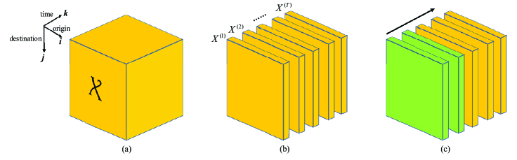
Figure 1: Third-order traffic tensor model. (a) Third-order traffic tensor $\mathcal{X}$, with the $(i,j,k)$-th element $x_{ijk}$ being the traffic flow transmitted from the $i$-th origin to $j$-th destination in the $k$-th time interval. (b) Different time intervals of $\mathcal{X}$, i.e., $X^{(1)},\cdots,X^{(T)}$. (c) The traffic tensor $\mathcal{X}$ is recovered as chronological order. The traffics in green have been recovered, while the traffics in yellow have not.

Consider the network consists of S nodes and the traffic information on T discrete time intervals, the dimension of traffic tensor $\mathcal{X}$ is $S\times S\times T$, and the dimension of its frontal slices, i.e. $X^{(1)},\cdots,X^{(T)}$ (see Figure 1 (b)), are all $S\times S$. If we further assume that the network has $M$ links and $N$ OD pairs, then $M,\ S$ and $N$ satisfy the following relations:

$$N^{1/2}=S\leq M+1<N.$$

The character of a large-scale network system is that the size of $M$ and $N$ could be very large. In addition, the network topology would be rather sparse ($S\approx M\ll N$). In the HOD network, there are 577 links, 243 nodes and 59049 OD pairs. More than 95% of OD pairs do not transmit any traffic.

In this work, we propose a fast and accurate recovery method for NTP. First, we develop a convex Sparsity Low-Rank Recovery (SLRR) model, which is the first to consider both spatial low-rank property and the sparsity of traffic data. Moreover, SLRR can be divided into a group of subproblems, each of which only related to the traffics in a single time interval. Thus, the problem scale can be sharply reduced, and we can recover the traffics as chronological order (see Figure 1 (c)). Then, we design a Schur Complement Based semi-proximal Alternating Direction Method of Multipliers (SCB-spADMM) to solve SLRR. For each block variable, we derive the explicit form of its optimum in the updating schemes. Thus, the algorithm iteration is rather fast and accurate. Based on Li, Sun and Toh’s research [21], the global convergence of SCB-spADMM is established. In addition, with the separable structure of SLRR, people can easily design the parallel algorithm. Finally, we utilize cross-validation, a commonly used strategy for parameter setting in machine learning, to previously pick out a group of appropriate parameters involved in our model and algorithm. Such a technique is data-independent, and thus it strengthens the robustness of our approach.

To test the accuracy and efficiency of numerical methods, we need practical network datasets. In this field, Abilene dataset and GEANT dataset are frequently used. Abilene/G$\rm\acute{E}$ANT dataset consists of 41/74 links and 11/23 nodes, collected using 5-minute/15-minute time intervals from Dec. 8, 2003 to Dec. 28, 2003/Jan. 1, 2005 to Apr. 29, 2005. However, the scale of these datasets is too small compared to the real network problems. Therefore, we released a new dataset – HOD dataset, which is extracted and modified from real data. The traffics of HOD network are collected in 671 time-intervals, each of which lasts for 15 minutes. There are 243 nodes and 577 links, and 95% of OD pairs never transmit traffic. Thus HOD traffic data is highly sparse. Since monitoring the OD traffics is prohibitively expensive, our HOD dataset does not contain such information. This means that HOD dataset is mainly applicable to NTP that this work cares about. We will see that the method proposed in this work is very effective for HOD dataset in Section 5. Furthermore, we also hope that the newly proposed HOD dataset can be used as the benchmark of traffic engineering methods in the future.

The outline of this paper is as follows. Our recovery model SLRR and SCB-spADMM algorithm are discussed in Section 2 and Section 3, respectively. In Section 4, we conduct numerical simulations and evaluate the performance of different approaches. In Section 5, we introduce the newly published HOD dataset and present the corresponding numerical simulations. In Section 6, the conclusion of our work is drawn.

2 Recovery Model

In this section, we first establish a regularized nuclear norm minimization with linear constraints, called Sparsity Low-Rank Recovery (SLRR) model, to infer the traffic data from link measurements. After analyzing the structure property of traffic data, we handle the traffic tensor $\mathcal{X}$ according to its frontal slices $X^{(1)},\cdots,X^{(T)}$. This improvement not only notably reduces the size of the problem but also makes it possible to design parallel algorithm. Then, we derive the dual model of SLRR, which can be easily solved by SCB-spADMM. Finally, the optimality conditions of the primal and dual problems are presented for setting the stopping criterion of SCB-spADMM.

2.1 Sparsity Low-Rank Recovery Model

Intuitively, the optimization model to recover the traffics in the $k$-th ($k=1,\cdots,T$) time interval $X^{(k)}$ with the spatial low-rank property can be established by minimizing the rank function:

$$\min\limits_{X^{(k)}} \text{rank}(X^{(k)})$$ (1)

s.t. $$\mathcal{A}_{k}(X^{(k)})=B_{k},$$

where $\mathcal{A}_{k}$ is a linear operator and $B_{k}$ contains measurements and other given constrains. Since rank function is nonconvex and nonsmooth, it is often relaxed by nuclear norm $\|\cdot\|_{*}$. It stands for the sum of all the singular values of a matrix, which is proved to be the tightest convex relaxation of rank function on the unit sphere $\mathcal{B}:=\{X:\ \|X\|_{2}\leq 1\}$ [11]. The linear constraint $\mathcal{A}_{k}(X^{(k)})=B_{k}$ contains three types of information:

1. $X^{(k)}$ is nonnegative.

2. The sparsity constraint of the complete traffic tensor takes form as $\mathcal{P}_{\Omega}(\mathcal{X})=0$, where $\Omega\subset\{(i,j,k):\ 1\leq i,j\leq S,\ 1\leq k\leq T\}$ is the index set indicating the location of these zero-traffics and $\mathcal{P}_{\Omega}(\cdot)$ is the projection on $\Omega$, i.e., $\mathcal{P}_{\Omega}(x_{ijk})=x_{ijk}$ if $(i,j,k)\in\Omega$, otherwise, $\mathcal{P}_{\Omega}(x_{ijk})=0$. Denote $\Omega^{(k)}:=\{(i,j):\ (i,j,k)\in\Omega\}$. Thus, in model (1), it follows that $P_{\Omega^{(k)}}(X^{(k)})=0$.

3. By link-load measurements, we have

   $$L^{(k)}=R\cdot\text{vec}(X^{(k)}),$$ (2)

   where $R\in\mathbb{R}^{M\times N}$ is the 0-1 routing matrix, indicating which link associates to which OD pairs (see Figure 2), $L^{(k)}\in\mathbb{R}^{M}$ is the $k$-th column of link measurements matrix $L$ and $\text{vec}(X^{(k)})$ is vectorization of the spatial matrix $X^{(k)}$. Formulation (2) can be easily rewritten as

   $$R\cdot\text{vec}(X^{(k)})=\sum\limits_{j=1}^{S}R_{j}X^{(k)}e_{j},$$

   where $R=[R_{1},R_{2},\cdots,R_{S}]$ is uniformly divided into $S$ parts along its columns and $e_{j}$ is the zero-vector except the $j$-th element being 1.

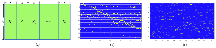
Figure 2: Routing matrix and its visualization. (a) Routing matrix $R$ and its blocks $R_{1},\cdots,R_{S}$. The dimensions of $R$ and each block $R_{i}(i\in\{1,\cdots,S\})$ are $m\times S^{2}$ and $M\times S$. (b) The routing matrix of Abilene dataset. (c) The routing matrix of G$\rm\acute{E}$ANT dataset. In (b) and (c), the blue elements are 0 while the yellow element are 1.

Therefore, we modify model (1) to (for simplicity but with a little ambiguity, we omit the index ‘(k)’):

$$\min\limits_{X} \|X\|_{*}$$

s.t. $$\sum\limits_{j=1}^{S}R_{j}Xe_{j}=L,\quad\mathcal{P}_{\Omega}(X)=0,\quad X\geq 0.$$

In internet traffic data, the variation of the traffics from the start to the end is often considerably large. Nevertheless, the traffics change slowly between adjacent time intervals. This continuity property of traffics has been studied in many models [26, 37, 43]. On the other hand, the traffics is also has periodic [37]. This situation of similar traffic in the same time period at different times can be understood as Internet users having similar behaviors in the same time period every day. By adding two regularized terms in model (2), we have obtained a more realistic model:

$$\min\limits_{X} \|X\|_{*}+\rho_{1}\|X-\bar{X}\|_{F}^{2}+\rho_{2}\|X-\hat{X}\|_{F}^{2}$$ (3)

s.t. $$\sum\limits_{j=1}^{S}R_{j}Xe_{j}=L,\quad\mathcal{P}_{\Omega}(X)=0,\quad X\geq 0.$$

Here, $\bar{X}$ and $\hat{X}$ represent the traffics one time interval ago, and one week ago, respectively. The regularization parameters $\rho_{i}>0\ (i=1,2)$ allow a tunable tradeoff between the spatial low-rank property, the continuity, and the periodicity of traffics.

Equation (3) leads to the Sparsity Low-Rank Recovery (SLRR) model. It allows us to cope with the traffics in each individual time interval as the chronological order $X^{(1)}\to X^{(2)}\to\cdots$, instead of the aggregate data. As shown in Figure 1(c), the green frontal slices represent the recovered traffic data, while the yellow ones are not. This character sharply reduces the variable size of each independent subproblem, and it correctly describes the basic requirement that the update traffics needs to be reported immediately each time when the lastest time slice ends, e.g., the congestion control [14] and real-time monitoring [33].

2.2 Dual Problem

We first reformulate SLRR model (3) as

$$\min\limits_{X}\quad\|X\|_{*}+\alpha\|Z\|_{F}^{2}$$ (4)

$$\text{s.t.}\quad\sum\limits_{j=1}^{S}R_{j}Xe_{j}=L,\quad\mathcal{P}_{\Omega}(X)=0,\quad X=Y,\quad X-A-Z=0,\quad Y\geq 0.$$

In model (4), it follows

$$\alpha:=\rho_{1}+\rho_{2}\quad\text{and}\quad A=\frac{\rho_{1}\bar{X}+\rho_{2}\hat{X}}{\rho_{1}+\rho_{2}}.$$ (5)

The Lagrangian function of (4) is

$$L(X,Y,Z;U,V,W,Q,G):=\|X\|_{*}+\alpha\|Z\|_{F}^{2}-\langle U,\mathcal{P}_{\Omega}(X)\rangle-\langle V,X-Y\rangle\\ -\langle W,X-A-Z\rangle-\langle Q,\sum\limits_{j=1}^{S}R_{j}Xe_{j}-L\rangle,$$

with the variable matrix $Y$ being nonnegative. Since the objective function of (4) are convex and all of constraints are linear, it has the strong duality, namely

$$\min\limits_{X,Y\geq 0,Z}\max\limits_{U,V,W,G}L(X,Y,Z;U,V,W,Q,G)\\ =\max\limits_{U,V,W,G}\min\limits_{X,Y\geq 0,Z}L(X,Y,Z;U,V,W,Q,G).$$

This property leads to the dual problem that is very easy to solve with the SCB-spADMM. Next, we derive the dual form through the following minimization problem:

$$\min\limits_{X,Y\geq 0,Z}L(X,Y,Z;U,V,W,Q,G):=\min\limits_{X,Y\geq 0,Z}L_{1}(X,Y,Z).$$

Note that $X,Y$ and $Z$ in $L_{1}(\cdot)$ are decoupled. Thus, the above problem can be divided into three smaller pieces associated to $X,\ Y$ and $Z$ and be solved successively.

The subproblem of $X$ is solved by

$$\min\limits_{X}\quad\|X\|_{*}-\langle\mathcal{P}_{\Omega}(U)+V+W+\sum\limits_{j=1}^{s}R_{j}^{T}Qe_{j}^{T},X\rangle\\ =\left\{\begin{aligned} 0&,\quad\|\mathcal{P}_{\Omega}(U)+V+W+\sum\limits_{j=1}^{S}R_{j}^{T}Qe_{j}^{T}\|_{2}\leq 1,\\ -\infty&,\quad\text{otherwise}.\end{aligned}\right.$$

The last equality holds according to the inequality $\langle A,B\rangle\leq\|A\|_{*}\|B\|_{2}.$ When nonzero $B$ is fixed, the equality can be attained for certain $A$ because $\|\cdot\|_{*}$ and $\|\cdot\|_{2}$ are dual norms.

In terms of $Y$, the subproblem can be easily fixed by

$$\min\limits_{Y\geq 0} \langle V,Y\rangle=\left\{\begin{aligned} 0&,\quad V\geq 0,\\ -\infty&,\quad\text{otherwise}.\end{aligned}\right.$$

The optimum of $Z$ can also be trivially obtained since we only need to solve a convex quadratic programming

$$\min\limits_{Z} \alpha\|Z\|_{F}^{2}+\langle W,Z\rangle=-\frac{\|W\|_{F}^{2}}{4\alpha}.$$

As a consequence, the dual model of (4) takes the following form, and with the strong duality, they are equivalent.

$$\min\limits_{U,V,W,Q,G}\quad\frac{1}{4\alpha}\left\|W-2\alpha A\right\|_{F}^{2}-\langle Q,L\rangle$$ (6)

$$\text{ s.t. }\quad\mathcal{P}_{\Omega}(U)+V+W+\sum\limits_{j=1}^{S}R_{j}^{T}Qe_{j}^{T}=G,\quad V\geq 0,\quad\|G\|_{2}\leq 1.$$

For later developments, we further rewrite problem (6) as

$$\min\limits_{U,V,W,Q,G}\quad\delta_{\mathbb{R}^{s\times s}_{+}}(V)-\langle Q,L\rangle+\delta_{\mathcal{B}}(G)+\frac{1}{4\alpha}\left\|W-2\alpha A\right\|_{F}^{2}$$ (7)

$$\text{ s.t. }\quad\mathcal{P}_{\Omega}(U)+V+W+\sum\limits_{j=1}^{S}R_{j}^{T}Qe_{j}^{T}=G,$$

where $\mathcal{B}:=\{X\in\mathbb{R}^{S\times S}:\ \|X\|_{2}\leq 1\}$, $\mathbb{R}^{s\times s}_{+}:=\{X\in\mathbb{R}^{S\times S}:\ X\geq 0\}$, and $\delta_{\mathcal{C}}(\cdot)$ is the indicator function on a closed convex set $\mathcal{C}$, i.e., $\delta_{\mathcal{C}}(x)=0$ if $x\in\mathcal{C}$, otherwise $\delta_{\mathcal{C}}(x)=+\infty$. The objective of (7) contains two blocks, namely

$$\text{block}_{1}:=\left(\delta_{\mathbb{R}^{s\times s}_{+}}(V)-\langle Q,L\rangle\right)\ \text{and}\ \text{block}_{2}:=\left(\delta_{\mathcal{B}}(G)+\frac{1}{4\alpha}\left\|W-2\alpha A\right\|_{F}^{2}\right),$$

each of which is a convex composite quadratic function. In general, a convex composite quadratic function takes form as

$$f(x,y)=p(x)+\langle y,My+b\rangle,$$

where $p(\cdot):\mathcal{X}\to(-\infty,+\infty]$ is closed proper convex function, $M$ is a positive semidefinite matrix and $b$ is a vector.

2.3 Optimality Condition and Stopping Criterion of Algorithm

The Karush-Kuhn-Tucker (KKT) conditions associated with (4) and (7) are given as follows.

$$\left\{\begin{aligned} &\sum\limits_{j=1}^{S}R_{j}Xe_{j}=L,\quad\mathcal{P}_{\Omega}(X)=0,\quad\mathcal{P}_{\Omega}(U)+V+W+\sum\limits_{j=1}^{S}R_{j}^{T}Qe_{j}^{T}=G,\\ &V\in\mathbb{R}^{S\times S}_{+},\quad G\in\mathcal{B}.\end{aligned}\right.$$

We can set the stopping criterion according to these KKT conditions. Specifically, define $\eta:=\max\{\eta_{P_{1}},\ \eta_{P_{2}},\ \eta_{D},\ \eta_{V},\ \eta_{G}\},$ where

$$\left\{\begin{aligned} &\eta_{P_{1}}:=\frac{\|\sum\limits_{j=1}^{S}R_{j}Xe_{j}-L\|_{F}}{1+\|L\|_{F}},\quad\eta_{P_{2}}:=\frac{\|\mathcal{P}_{\Omega}(X)\|_{F}}{1+\|X\|_{F}},\\ &\eta_{D}:=\frac{\|\mathcal{P}_{\Omega}(U)+V+W+\sum\limits_{j=1}^{S}R_{j}^{T}Qe_{j}^{T}-G\|_{F}}{1+\|G\|_{F}},\\ &\eta_{V}:=\frac{\|V-\mathcal{P}_{\mathbb{R}^{S\times S}_{+}}(V)\|_{F}}{1+\|V\|_{F}},\quad\eta_{G}:=\frac{\|G-\mathcal{P}_{\mathcal{B}}(G)\|_{F}}{1+\|G\|_{F}}.\end{aligned}\right.$$

We can set a small positive parameter $\varepsilon$ and stop the algorithm when $\eta<\varepsilon$ or the iteration step attains it maximum.

3 Schur Complement Based Semi-Proximal ADMM

Next, we would develop the Schur Complement Based semi-proximal ADMM (SCB-spADMM) for (7). As it is well known, the ADMM-type algorithm is effective and efficient for large-scale convex modes with linear constraints [3, 8, 9, 21] and has been successfully applied to many nuclear norm minimization problems [32, 24, 22]. It is easy to implement and only requires little memory space. The convergence of our SCB-spADMM can be similarly proved as in [21]. In particular, the optimum of each variable can be solved explicitly.

3.1 Traditional Multi-Block ADMM

A natural idea is to directly employ a 5-block ADMM for solving model (7). Denote

$$\Gamma(U,V,W,Q,G):=\mathcal{P}_{\Omega}(U)+V+W+\sum\limits_{j=1}^{S}R_{j}^{T}Qe_{j}^{T}-G.$$

The Lagrangian function of (7) is

$$L_{\beta}(U,V,W,Q,G;X):=\delta_{\mathbb{R}^{S\times S}_{+}}(V)-\langle Q,L\rangle+\delta_{\mathcal{B}}(G)+\frac{1}{4\alpha}\left\|W-2\alpha A\right\|_{F}^{2}\\ +\langle X,\Gamma(U,V,W,Q,G)\rangle+\frac{\beta}{2}\|\Gamma(U,V,W,Q,G)\|_{F}^{2}.$$

A commonly used algorithm for solving (7) is the directly extended 5-block ADMM. Its iteration steps are given by

$$\left\{\begin{aligned} &U^{k+1}:=\arg\min_{U}L_{\beta}(U,V^{k},W^{k},Q^{k},G^{k};X^{k}),\\ &V^{k+1}:=\arg\min_{V}L_{\beta}(U^{k+1},V,W^{k},Q^{k},G^{k};X^{k}),\\ &W^{k+1}:=\arg\min_{W}L_{\beta}(U^{k+1},V^{k+1},W,Q^{k},G^{k};X^{k}),\\ &Q^{k+1}:=\arg\min_{Q}L_{\beta}(U^{k+1},V^{k+1},W^{k+1},Q,G^{k};X^{k}),\\ &G^{k+1}:=\arg\min_{G}L_{\beta}(U^{k+1},V^{k+1},W^{k+1},Q^{k+1},G;X^{k}),\\ &X^{k+1}:=X^{k}+\tau\beta(\mathcal{P}_{\Omega}(U^{k+1})+V^{k+1}+W^{k+1}+\sum\limits_{j=1}^{s}R_{j}^{T}Q^{k+1}e_{j}^{T}-G^{k+1}).\end{aligned}\right.$$

Since each variable can be obtained explicitly in the iterations, the solving of subproblems becomes very simple. On the other hand, as mentioned in [7], it is a challenge to ensure that the designed multi-block ($\geq 3$ blocks) ADMM is convergent. This is a difficulty we need to overcome.

Inspired by Li, Sun and Toh’s impressive work [21], we will propose a convergent ADMM algorithm below. By introducing the proximal or semi-proximal terms, the subproblems in the proximal ADMM (pADMM) or semi-proximal ADMM (spADMM) can be solved efficiently. Thus they are more suitable to cope with convex composite quadratic programmings and convex quadratic conic programmings. The key point of designing the semi proximal term in SCB-spADMM is to modify the algorithm into the split version based on Gauss-Seidel type decomposition.

Algorithm SCB-spADMM for solving (7)

  Define $R_{j}$ as the $j-$th block of the routing matrix $R$, and $e_{j}$ as the zero vector except the $j$-th element being one. Calculate $\alpha$ and $A$ through (5). Choose $U^{0},\ Q^{0},\ V^{0},\ W^{0},\ G^{0},\ X^{0}$ as zero matrices. For $k=0,1,\cdots,$ repeat the following iteration scheme.

  while Stopping criterion is not reached do

     Update $U,\ Q$ and $V$ as the following order according to formulations (11), (12), (14), respectively.              

$$\left\{\begin{aligned} &U^{k+\frac{1}{2}}:=\arg\min\limits_{U}L_{\beta}(U,Q^{k},V^{k},W^{k},G^{k};X^{k})+\frac{\beta}{2}\|U-U^{k}\|_{\mathcal{H}_{U}}^{2},\\ &Q^{k+\frac{1}{2}}:=\arg\min\limits_{Q}L_{\beta}(U^{k+\frac{1}{2}},Q,V^{k},W^{k},G^{k};X^{k})+\frac{\beta}{2}\|Q-Q^{k}\|_{\mathcal{H}_{Q}}^{2},\\ &V^{k+1}:=\arg\min\limits_{V}L_{\beta}(U^{k+\frac{1}{2}},Q^{k+\frac{1}{2}},V,W^{k},G^{k};X^{k})+\frac{\beta}{2}\|V-V^{k}\|_{\mathcal{H}_{V}}^{2},\\ &Q^{k+1}:=\arg\min\limits_{Q}L_{\beta}(U^{k+\frac{1}{2}},Q,V^{k+1},W^{k},G^{k};X^{k})+\frac{\beta}{2}\|Q-Q^{k+\frac{1}{2}}\|_{\mathcal{H}_{Q}}^{2},\\ &U^{k+1}:=\arg\min\limits_{U}L_{\beta}(U,Q^{k+1},V^{k+1},W^{k},G^{k};X^{k})+\frac{\beta}{2}\|U-U^{k+\frac{1}{2}}\|_{\mathcal{H}_{U}}^{2},\\ \end{aligned}\right.$$ (8)

Update $W$ and $G$ as the following order according to formulations (13), (15), respectively.              

$$\left\{\begin{aligned} &W^{k+\frac{1}{2}}:=\arg\min\limits_{W}L_{\beta}(U^{k+1},Q^{k+1},V^{k+1},W,G^{k};X^{k})+\frac{\beta}{2}\|W-W^{k}\|_{\mathcal{H}_{W}}^{2},\\ &G^{k+1}:=\arg\min\limits_{G}L_{\beta}(U^{k+1},Q^{k+1},V^{k+1},W^{k+\frac{1}{2}},G;X^{k})+\frac{\beta}{2}\|G-G^{k}\|_{\mathcal{H}_{G}}^{2},\\ &W^{k+1}:=\arg\min\limits_{W}L_{\beta}(U^{k+1},Q^{k+1},V^{k+1},W,G^{k+1};X^{k})+\frac{\beta}{2}\|W-W^{k+\frac{1}{2}}\|_{\mathcal{H}_{W}}^{2},\\ \end{aligned}\right.$$ (9)

$X^{k+1}:=X^{k}+\gamma\beta(P_{\Omega}(U^{k+1})+V^{k+1}+W^{k+1}+\sum\limits_{j=1}^{s}R_{j}^{T}Q^{k+1}e_{j}^{T}-G^{k+1}).$

  end while

  return  $X$

3.2 Algorithm Framework

As introduced in [21], let $\mathcal{H}_{U},\ \mathcal{H}_{Q},\ \mathcal{H}_{W},\ \mathcal{H}_{V}$ and $\mathcal{H}_{G}$ be self-adjoint positive semidefinite linear operators and satisfy

$$\mathcal{H}_{U}:=\mathcal{G}_{U}-P_{\Omega}^{*}P_{\Omega}=\mathcal{G}_{U}-P_{\Omega},\quad\mathcal{H}_{Q}:=\mathcal{G}_{Q}-\mathcal{A}^{*}\mathcal{A},$$ (10)

$$\mathcal{H}_{W}:=\mathcal{G}_{W}-\frac{1}{\beta}\mathcal{I}-\mathcal{I}^{*}\mathcal{I}=\mathcal{G}_{W}-(\frac{1}{\beta}+1)\mathcal{I},$$

$$\mathcal{H}_{V}:=\mathcal{G}_{V}-\mathcal{I}^{*}\mathcal{I}=\mathcal{G}_{V}-\mathcal{I},\quad\mathcal{H}_{G}:=\mathcal{G}_{G}-\mathcal{I}^{*}\mathcal{I}=\mathcal{G}_{G}-\mathcal{I},$$

where $\mathcal{G}_{U},\ \mathcal{G}_{Q},\ \mathcal{G}_{W},\ \mathcal{G}_{V}$ and $\mathcal{G}_{G}$ are also self-adjoint positive semidefite linear operators, and additionally, their inverses are relatively easy to compute. $\mathcal{A}$ is a linear operator satisfying $\mathcal{A}Q:=\sum\limits_{j=1}^{s}R_{j}^{T}Qe_{j}^{T}$ and $\mathcal{I}$ is the identity operator, i.e., $\mathcal{I}X=X$ for any $X$. From the definition, we can derive that $\mathcal{A}^{*}\mathcal{A}Q=\sum\limits_{j=1}^{s}R_{j}R_{j}^{T}Q.$ We propose the SCB-spADMM algorithm for solving model (7) as in Algorithm Algorithm.

3.3 Convergence

The presence of $\mathcal{H}_{U},\ \mathcal{H}_{Q},\ \mathcal{H}_{W},\ \mathcal{H}_{V}$ and $\mathcal{H}_{G}$ can guarantee the existence of the solution of subproblem (8) and (9), as well as the boundedness of the iteration points $U^{k},\ Q^{k},\ W^{k},\ V^{k}$ and $G^{k}$. In general, $\mathcal{H}_{U},\ \mathcal{H}_{Q},\ \mathcal{H}_{W},\ \mathcal{H}_{V}$ and $\mathcal{H}_{G}$ should be as small as possible and meanwhile $U^{k},\ Q^{k},\ W^{k},\ V^{k}$ and $G^{k}$ are still easy to compute. According to [21], we have the following convergence result.

Theorem 3.1.

If one of (1) $\tau\in(0,\frac{\sqrt{5}+1}{2})$ and (2) $\tau\geq\frac{\sqrt{5}+1}{2}$ but $\sum\limits_{k=0}^{+\infty}\|(G^{k+1}-G^{k})+(W^{k+1}-W^{k})\|_{F}^{2}+\frac{1}{\tau}\|\mathcal{P}_{\Omega}(U^{k+1})+V^{k+1}+W^{k+1}+\sum\limits_{j=1}^{s}R_{j}^{T}Q^{k+1}e_{j}^{T}-G^{k+1}\|_{F}^{2}<+\infty$, then we have the following properties.

1. $U^{k},$ $Q^{k}$, $W^{k}$, $V^{k}$ and $G^{k}$ are automatically well defined based on the settings of $\mathcal{H}_{U}$, $\mathcal{H}_{Q},\ \mathcal{H}_{W},$ $\mathcal{H}_{V}$ and $\mathcal{H}_{G}$ given by (10).

2. $\{(U^{k},\ Q^{k},\ W^{k}$, $V^{k},\ G^{k},\ X^{k})\}_{k=1}^{\infty}$ converges to the unique accumulate point $(U^{\infty},\ Q^{\infty},\ W^{\infty},\ V^{\infty},$ $G^{\infty},\ X^{\infty})$, with $(U^{\infty},\ Q^{\infty},\ W^{\infty},\ V^{\infty},\ G^{\infty})$ being the optimum of model (7) and $X^{\infty}$ being the optimum of model (4).

Proof.

After substituting the specific form of (7), it becomes a straightforward deduction of Theorem 3 in [21]. $\Box$ ∎

Recall the requirements of $\mathcal{H}_{U},\ \mathcal{H}_{Q},\ \mathcal{H}_{W},\ \mathcal{H}_{V}$ and $\mathcal{H}_{G}$ introduced previously, we can simply set $\mathcal{H}_{W}=\mathcal{H}_{V}=\mathcal{H}_{G}={\bf 0}$ if we let $\mathcal{G}_{V}=\mathcal{G}_{G}=(\frac{1}{\beta}+1)^{-1}\mathcal{G}_{W}=\mathcal{I}.$ Since $\mathcal{P}_{\Omega}$ is a nondegenerate projection operator, it follows that $\|\mathcal{P}_{\Omega}\|_{2}=1$. Thus, we can set $\mathcal{G}_{U}=\mathcal{I}$ and have $\mathcal{H}_{U}=\mathcal{I}-\mathcal{P}_{\Omega}.$ In terms of $\mathcal{H}_{Q}$, from the equation $\mathcal{A}^{*}\mathcal{A}Q=\sum\limits_{j=1}^{S}R_{j}R_{j}^{T}Q$, we know that $\|\mathcal{A}^{*}\mathcal{A}\|_{2}=\|\sum\limits_{j=1}^{S}R_{j}R_{j}^{T}\|_{2}.$ As for $\mathcal{G}_{Q}$, a common and simple setting is $\mathcal{G}_{Q}=\lambda_{\text{max}}\mathcal{I}$, where $\lambda_{\text{max}}$ is the largest eigenvalue of $\mathcal{A}^{*}\mathcal{A}$. Thus, we have that

$$\mathcal{H}_{Q}(Q)=(\lambda_{\text{max}}I-\sum\limits_{j=1}^{S}R_{j}R_{j}^{T})Q:=H_{Q}Q.$$

In the following, we will derive the explicit forms of the subproblems associated to $U,\ Q,\ V,\ W$ and $G$, respectively.

The subproblem of $U$ takes the form as

$$\min\limits_{U}\ \langle X,P_{\Omega}(U)\rangle+\frac{\beta}{2}\|\Gamma(U,V,W,Q,G)\|_{F}^{2}+\frac{\beta}{2}\|U-U^{k}\|_{\mathcal{I}-\mathcal{P}_{\Omega}}^{2}.$$

Since it is an unconstraint model and its objective function is convex and differentiable, we can obtain its optimum by directly setting the gradient of the objective function to zero. Thus, the optimum of $U$ is

$$U^{*}:=\mathcal{P}_{\Omega}\left(-V-\sum\limits_{j=1}^{S}R_{j}^{T}Qe_{j}^{T}-W+G-\frac{X}{\beta}\right)+\mathcal{P}_{\Omega^{\text{C}}}(U^{k}),$$ (11)

Similarly, we can simply derive the optimum of $Q$ and $W$ by

$$Q^{*}:= \arg\min\limits_{Q}\ \langle\sum\limits_{j=1}^{S}R_{j}Xe_{j}-L,Q\rangle+\frac{\beta}{2}\|\Gamma(U,V,W,Q,G)\|_{F}^{2}+\frac{\beta}{2}\|Q-Q^{k}\|_{H_{Q}}^{2}$$ (12)

$$= -\frac{1}{\lambda_{\text{max}}}\left(\sum\limits_{j=1}^{S}R_{j}(V+P_{\Omega}(U)+W-G)e_{j}-H_{Q}Q^{k}+\frac{\sum\limits_{j=1}^{s}R_{j}Xe_{j}-L}{\beta}\right)$$

and

$$W^{*}:= \arg\min\limits_{W}\ \frac{1}{4\alpha}\|W-2\alpha A\|_{F}^{2}+\langle X,W\rangle+\frac{\beta}{2}\|\Gamma(U,V,W,Q,G)\|_{F}^{2}$$ (13)

$$= \frac{A-X-\beta\left(V+\sum\limits_{j=1}^{S}R_{j}^{T}Qe_{j}^{T}+P_{\Omega}(U)-G\right)}{\frac{1}{2\alpha}+\beta}.$$

The subproblem in terms of $V$ can be divided into a group of convex quadratic programmings, each of which asks for nonnegative solution and associates to scalar variable. It is easy to derive that

$$V^{*}:= \arg\min\limits_{V}\ \delta_{\mathbb{R}^{S\times S}_{+}}(V)+\langle X,V\rangle+\frac{\beta}{2}\|\mathcal{P}_{\Omega}(U)+V+W+\sum\limits_{j=1}^{s}R_{j}^{T}Qe_{j}^{T}-G\|_{F}^{2}$$ (14)

$$= \max\left\{0,-\left(\sum_{j=1}^{s}R_{j}^{T}Qe_{j}^{T}+P_{\Omega}(U)+W-G\right)-\frac{X}{\beta}\right\}.$$

About $G$, suppose $\ U_{G}\Sigma_{G}V_{G}:=V+\sum R_{j}^{T}Qe_{j}^{T}+P_{\Omega}(U)+W-\frac{X}{\beta}$ is the economical singular value decomposition (SVD). Then, we have that

$$G^{*}:= \arg\min\limits_{G}\ \delta_{\mathcal{B}}(G)-\langle X,G\rangle+\frac{\beta}{2}\|\Gamma(U,V,W,Q,G)\|_{F}^{2}$$ (15)

$$= U_{G}\min\left\{I,\Sigma_{G}\right\}V_{G}^{T}.$$

4 Numerical Simulations

In this section, we present the simulation results of our SLLR model and SCH-spADMM algorithm on the Abilene and GEANT datasets. The results of Tomo-SRMF [26], SDPLR [24] and Tomo-Gravity [42] are also output for comparison. As already mentioned in the introduction section, we will focus on more practical network tomography problem [1, 24, 26, 31, 40, 41] here rather than the completion problem [5, 6, 15, 24, 26, 34, 35, 37, 38, 39, 43].

We notice there are some anomalies in G$\rm\acute{E}$ANT traffics [30]. As seen in Figure 3, a few of traffic volumes are much larger than the others. Suppose the traffics in the time intervals $t_{1}$ and $t_{2}$ are correct but all the intermediate traffics are abnormal. Then, we modify the anomalies by using linear interpolation between the time intervals $t_{1}$ and $t_{2}$. In Figure 3 (c), the refined data is presented. For Abilene dataset, we can see that it has good quality from Figure 4. Thus no special processing is required.

As previously mentioned, the real-world traffic data is of high sparsity. In order to imitate this realistic circumstance, we modify the Abilene dataset and G$\rm\acute{E}$ANT dataset by setting the smallest $p\%\ (p=50,70,90)$ of OD pairs to zero-ODs, which means they do not transmit any network traffic.

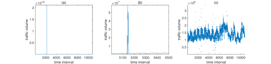
Figure 3: The Frobenius norm of (a) the original G$\rm\acute{E}$ANT traffics in each time interval, (b) the original G$\rm\acute{E}$ANT traffics from the 5001st time interval to the 5500th time interval, (c) the modified G$\rm\acute{E}$ANT traffics in each time interval.

K-fold [23] Cross Validation (CV) is employed to find proper parameters $(\alpha_{1},\alpha_{2},\beta)$ in our algorithm. We uniformly divide the rows of the link-measurement matrix $L$ into $K$ groups. Each row group and the traffics therein are denoted as $\Psi_{l}$ and $L_{\Psi_{l}}$ $(l=1,\cdots,K)$, respectively. Then, we generate candidate parameters $\{(\alpha_{1}^{j},\alpha_{2}^{j},\beta^{j})\}_{j=1}^{1000}$ from a wide-range interval. All of candidates will be evaluated by the following steps:

1. Let the integer $l$ change from 1 to $K$. In each case, $L_{\Psi_{l}}$ is taken as the test set, while the other link-load data is taken as the training set.

2. Based on the link-load traffics in the training set, we can obtain an estimation of the traffics in rows $\Psi_{l}$ using proposed SCB-spADMM, denoted as $\hat{L}_{\Psi_{l}}$.

3. If $l=K$, calculate the overall recovery error by Normalized Mean Absolute Error (NMAE) for CV, defined as

   $$\text{N}_{\text{CV}}:=\frac{\sum\limits_{l=1}^{K}\sum\limits_{i\in\Psi_{l}}\sum\limits_{j=1}^{T}\left|(\hat{L}_{\Psi_{l}})_{ij}-(L_{\Psi_{l}})_{ij}\right|}{\sum\limits_{i=1}^{M}\sum\limits_{j=1}^{T}L_{ij}}.$$

Ultimately, we choose the candidate that corresponds to the lowest $\text{N}_{\text{CV}}$ as the parameters used in our algorithm. With the fixed parameters, we can implement SCB-spADMM to estimate the whole OD traffics. The recovery performance is evaluated by NMAE on the missing data:

$$\text{NMAE}:=\frac{\sum\limits_{(i,j,k)\in\Omega^{C}}|\hat{\mathcal{X}}_{ijk}-\mathcal{X}_{ijk}|}{\sum\limits_{(i,j,k)\in\Omega^{C}}\mathcal{X}_{ijk}},$$ (16)

We compare SLRR against three alternative methods: Tomo-SRMF, SDPLR and Tomo-Gravity. The complete three-week Abilene traffics and four-month G$\rm\acute{E}$ANT traffics are simulated. In particular, we simulate G$\rm\acute{E}$ANT dataset in three different time periods: the first week, the first eight weeks and the last eight weeks, respectively. We need to point out that other work [26, 43] only simulated the one-week data of the GEANT dataset. In fact, sometimes people only care about one-week traffics rather than the aggregate data.

The simulation results are reported in Table 1. We can see that as the sparsity increases, the recovery errors will decrease. This is because high sparsity contains more raw traffic information and reduce uncertainty. More importantly, our SLRR is significantly better than other methods in all cases. For the GEANT dataset, the results of the first-week data are better than the results of the other two groups. This may be related to the data quality of the GEANT dataset. Nevertheless, our SLRR is still superior to other methods in these cases.

Table 1: Comparison of NMAE on Abilene and G$\rm\acute{E}$ANT datasets. For G$\rm\acute{E}$ANT dataset, we output the simulation results of the first-week/the first-eight-week/the last-eight-week data.

Method	Sparsity = 50%	Sparsity = 70%	Sparsity = 90%
	Abilene
Tomo-SRMF	0.374	0.335	0.236
SDPLR	0.535	0.393	0.272
Tomo-Gravity	0.631	0.558	0.248
SLRR	0.193	0.136	0.047
	G$\rm\acute{E}$ANT
Tomo-SRMF	1.003/1.182/1.342	0.725/0.922/1.075	0.271/0.465/0.530
SDPLR	1.004/1.055/1.171	0.734/0.859/0.973	0.308/0.456/0.526
Tomo-Gravity	1.065/1.113/1.145	0.871/0.971/1.005	0.583/0.644/0.734
SLRR	0.640/0.743/0.792	0.444/0.590/0.639	0.124/0.271/0.337

The recovery performances of SLRR in different time intervals are presented in Figure 4. We especially mark the NAME under certain sparsity with a horizontal dashed line of the same color. It shows that our recovery results are consistent and reliable.

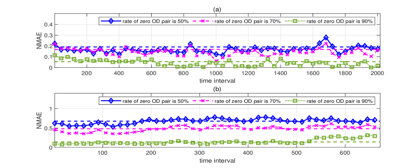
Figure 4: NMAE in different time intervals on (a) the complete three-week traffics of Abilene dataset, (b) the first-week traffics of G$\rm\acute{E}$ANT dataset. The spaces between adjacent time intervals are 40 for Abilene dataset and 15 for G$\rm\acute{E}$ANT dataset.

5 The HOD Dataset and Simulations

Compared with Abilene dataset and GEANT dataset, the most significant feature of HOD dataset is that it is highly sparsity. In fact, 95.26% of OD pairs have no traffic. In Figure 5, we fully demonstrate this. Moreover, HOD dataset also has continuity and periodicity, see Figure 6 for illustration. In the following simulations, we will also make use of these properties.

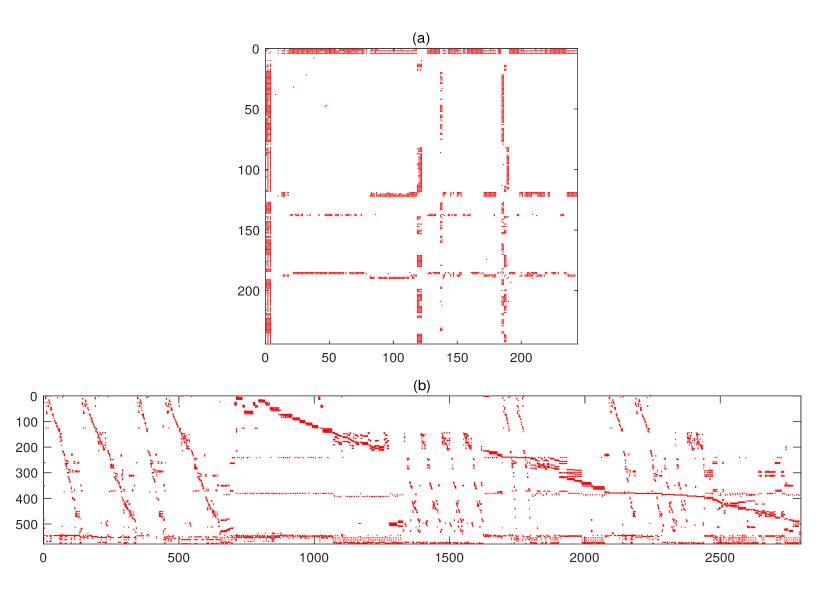
Figure 5: The sparsity of (a) the spatial matrix, (b) the routing matrix of HOD dataset. The red components in the spatial matrix means that the corresponding OD pairs have transmitted traffic data, and those in the routing matrix stand for 1-components.

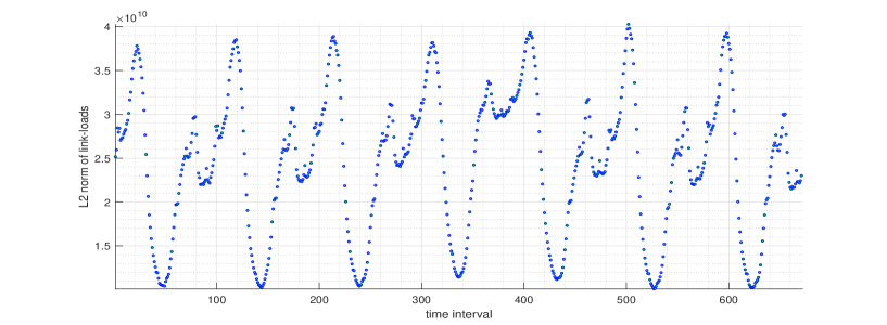
Figure 6: The Frobenius norm of link-loads in different time intervals. The figure illustrates the the continuity and the periodicity of HOD dataset.

Next, we evaluate different methods on HOD dataset. Because the real OD traffics are unclear, NMAE metric (16) is no longer effective. Again we utilize CV errors (3) for assessment. Except the aforementioned K-fold CV, we also consider another kind of CV, named the Monte Carlo CV [10] to make fair evaluation. In the Monte Carlo CV, the training set and the test set are randomly generated. We set the ratio of the test sets to 2% and repeat 50 times in each simulation.

Table 2 presents the recovery performance of different methods testing on HOD dataset. ‘SLRR-MC’ stands for the case where SLRR is evaluated by Monte Carlo CV. From Table 2, we find that over the four methods, SLRR significantly outperforms the others. Moreover, the recovery results of SLRR assessed by two different CVs are very close.

Table 2: Comparison of recovery performance on HOD dataset.

Method	Tomo-SRMF	SDPLR	Tomo-Gravity	SLRR	SLRR-MC
NMAE	0.3314	0.2832	0.3243	0.1588	0.1519

The computational time of our algorithm is also investigated. The overall simulations are implemented on an ASUS laptop (4-core, Intel i7-10510U, @2.30GHz, 16G RAM). We have to admit that our SLRR model is slower than the other methods due to the SVD decomposition. However, our method only takes a few seconds (see Figure 7) to recover the time interval of more than ten minutes in practical scenarios. This well satisfies the requirement of practical problems. Moreover, our SLRR model has better recovery accuracy than all the existing methods in any case. These make our SLRR model have significant advantages in the network tomography problem, and it may be integrated into future products.

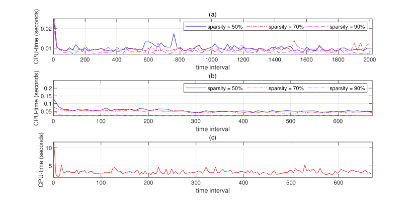
Figure 7: CPU-time of each time interval on (a) Abilene dataset, (b) G$\rm\acute{E}$ANT dataset, (c) HOD dataset. For Abilene and G$\rm\acute{E}$ANT datasets, it takes less than 0.1 second to recover the traffics in one time interval. For large-scale HOD dataset, it also only takes several seconds for each interval.

6 Conclusions

Our research extends the knowledge into solving large-scale network tomography problem. By leveraging on the spatial low-rank property and the sparsity of traffic data, we propose SLRR model to accurately inference the network traffics. The separability of SLRR can significantly reduce the problem scale and make it possible to design parallel algorithm. To solve SLRR, we design a globally convergent Schur complement based semi-proximal alternating direction method of multipliers. Since all of optimums of block variables can be calculated by explicit forms, the iteration scheme is fast and accurate. K-fold cross validation is employed to find proper parameters in our algorithm. By taking advantages of the above techniques, our method outperforms all the others with respect to the recovery accuracy. Moreover, the seconds-feedback on different datasets also demonstrate the high computation efficiency of our algorithm. Except the proposed methodology, another highlight of our work is that we publish an industrial dataset HOD to enrich the database of network traffics recovery study.

References

- [1] Gunnar, A., Johansson, M., Telkamp T. Traffic matrix estimation on a large IP backbone: a comparison on real data. In: Proceedings of the 4th ACM SIGCOMM conference on internet measurement. ACM. 149–160 (2004)
- [2] Benson, T., Akella, A., Maltz, D. Network traffic characteristics of data centers in the wild. In: Proceedings of the 10th Acm Sigcomm Conference on Internet Measurement. ACM. 267–280 (2010)
- [3] Boyd, S., Parikh, N., Chu, E., et al. Distributed Optimization and Statistical Learning via the Alternating Direction Method of Multipliers. Foundations & Trends in Machine Learning. 3, 1–122 (2010)
- [4] Cahn, R.S. Wide area network design: concepts and tools for optimization. IEEE Press. 38, 28–30 (2000)
- [5] Candes, E.J., Tao, T. The power of convex relaxation: near-optimal matrix completion. IEEE Trans. Inf. Theory. 56, 2053–2080 (2010)
- [6] Chen, C.H., He, B.S., Yuan, X.M. Matrix completion via an alternating direction method. IMA. J Numer. Anal. 32, 227–245 (2012)
- [7] Chen, C.H., He, B.S., Ye, Y.Y., et al. The direct extension of ADMM for multi-block convex minimization problems is not necessarily convergent. Math. Program. 155, 57–79 (2014)
- [8] Chen, L., Li, X.D., Sun, D.F., et al. On the equivalence of inexact proximal ALM and ADMM for a class of convex composite programming. Math. Program. (2019) https://doi.org/10.1007/s10107-019-01423-x
- [9] Chen, L., Sun, D.F., Toh, K.C. An efficient inexact symmetric Gauss–Seidel based majorized ADMM for high-dimensional convex composite conic programming. Math. Program. 161, 237–270 (2016)
- [10] Dubitzky, W., Granzow, M., Berrar, D. Fundamentals of Data Mining in Genomics and Proteomics. Springer, Boston, MA (2007)
- [11] Fazel, M. Matrix rank minimization with applications. Dissertation for the Doctoral Degree. San Francisco: Stanford University. 63–04 (2002)
- [12] Fortz, B., Thorup, M. Optimizing OSPF/IS-IS weights in a changing world. IEEE Journal on selected in communications. 20, 756–767 (2002)
- [13] Hong, C.Y., Liang, S., Mendelev, K., et al. B4 and after: managing hierarchy, partitioning, and asymmetry for availability and scale in google’s software-defined WAN. In: Proceedings of the 2018 Conference of the ACM Special Interest Group on data communication. ACM. 74–87 (2018)
- [14] Jacobson, V. Congestion avoidance and control. ACM SIGCOMM computer communication review. 18, 314–329 (1988)
- [15] Jiang, D.D., Wang, W.J., Shi, L., et al. A compressive sensing-based approach to end-to-end network traffic reconstruction. IEEE transactions on network science and engineering. 7: 507–519 (2020)
- [16] Kiers, H.A.L. Towards a standardized notation and terminology in multiway analysis. J Chemometr. 14, 105–122 (2000)
- [17] Kilmer, M.E., Martin, C.D. Factorization strategies for third-order tensors. Linear Alg Appl. 435, 641–658 (2011)
- [18] Kruskal, J.B. Rank, decomposition, and uniqueness for 3-way and N-way arrays. Multiway data analysis. 7–18 (1989)
- [19] Nie, L. S., Jiang, D., Guo, L. A compressive sensing-based approach to end-to-end network traffic reconstruction utilising partial measured origin-destination flows. Trans Emerg Telecommun Technol. 26, 1108–1117 (2015)
- [20] Lakhina, A., Papagiannaki, K., Crovella, M., et al. Structural analysis of network traffic flows. Performance Evaluation Review. 32, 61–72 (2004)
- [21] Li, X.D., Sun, D.F., Toh, K.C. A Schur complement based semi-proximal ADMM for convex quadratic conic programming and extensions. Math. Program. 155, 333–373 (2016)
- [22] Lu, L.F, Huan, Z.Z., Zhang, X.Y., et al. Collaborative network traffic analysis via alternating direction method of multipliers. In: 2018 IEEE 22nd International Conference on Computer Supported Cooperative Work in Design ((CSCWD)). IEEE. 547-552 (2018)
- [23] McLachlan, G.J., Do, K.A., Ambroise, C. Analyzing microarray gene expression data. John Wiley & Sons Press. (2005)
- [24] Recht, B., Fazel, M., Parrilo, P.A. Guaranteed minimum-rank solutions of linear matrix equations via nuclear norm minimization. SIAM Rev. 52, 471–501 (2010)
- [25] Oseledets, I.V. Tensor-train decomposition. SIAM J Sci. Comput. 33, 2295–2317 (2011)
- [26] Roughan, M., Zhang, Y., Willinger, W., et al. Spatio-temporal compressive sensing and internet traffic matrices (extended version), IEEE/ACM Transactions on Networking. 20, 662–676 (2012)
- [27] Song, H., Dharmapurikar, S., Turner, J., et al. Fast hash table lookup using extended bloom filter: an aid to network processing. ACM SIGCOMM Computer Communication Review. 35, 181–192 (2005)
- [28] Tucker, L.R. Some mathematical notes on three-mode factor analysis. Psychometrika. 31, 279–311 (1966)
- [29] Tune, P., Roughan, M., Haddadi, H., et al. Internet traffic matrices: A primer. Recent Advances in Networking. 1, 1–56 (2013)
- [30] Uhlig, S., Quoitin, B., Lepropre, Jean., et al. Providing Public Intradomain Traffic Matrices to the Research Community. Association for Computing Machinery. 36, 83–86 (2006)
- [31] Vardi, Y. Network tomography: Estimating source-destination traffic intensities from link data. J Am. Stat. Assoc. 91, 365–377 (1996)
- [32] Wen, Z., Yin, W., Zhang, Y. Solving a low-rank factorization model for matrix completion by a nonlinear successive over-relaxation algorithm. Math. Program. Comput. 4, 333–361 (2012)
- [33] Wiseman, Y. Real-time monitoring of traffic congestions. 2017 IEEE International Conference on Electro Information Technology (EIT). Lincoln. NE. 501–505 (2017)
- [34] Xie, K., Li, X., Wang, X., et al. Fast tensor factorization for accurate internet anomaly detection. IEEE/ACM transactions on networking. 25: 3794–3807 (2017)
- [35] Xie, K., Li, X., Wang, X., et al. Active sparse mobile crowd sensing based on matrix completion. In: Proceedings of the 2019 International Conference on Management of Data. 195–210 (2019)
- [36] Xie, K., Tian, J., Wang, X., et al. Efficiently inferring top-k elephant flows based on discrete tensor completion. In: IEEE INFOCOM 2019-IEEE Conference on Computer Communications. 2170–2178 (2019)
- [37] Xie, K., Peng, C., Wang, X., et al. Accurate recovery of internet traffic data under dynamic measurements. In: IEEE INFOCOM 2017-IEEE Conference on Computer Communications. 1–9 (2017)
- [38] Xie, K., Wang, L., Wang, X., et al. Sequential and adaptive sampling for matrix completion in network monitoring systems. In: 2015 IEEE Conference on Computer Communications (INFOCOM). 2443–2451 (2015)
- [39] Xie, K., Wang, X., Wang, X., et al. Accurate recovery of missing network measurement data with localized tensor completion. IEEE/ACM Transactions on Networking. 27, 2222–2235 (2019)
- [40] Yu, B., Cao, J., Davis, D., et al. Time-varying network tomography: router link data. In: 2000 IEEE International Symposium on Information Theory (Cat. No. 00CH37060). 95, 1063–1075 (2000)
- [41] Zhang, Y., Roughan, M., Duffield, N., et al. Fast accurate computation of large-scale IP traffic matrices from link loads. ACM SIGMETRICS Performance Evaluation Review. 31, 206–217 (2003)
- [42] Zhang, Y., Roughan, M., Lund, C., et al. Estimating point-to-point and point-to-multipoint traffic matrices: An information-theoretic approach. IEEE/ACM Transactions on networking. 13, 947–960 (2005)
- [43] Zhou, H., Zhang, D., Xie, K., et al. Spatio-temporal tensor completion for imputing missing internet traffic data. In: 2015 IEEE 34th International Performance Computing and Communications Conference (IPCCC). 1–7 (2015)