Cross-domain Activity Recognition via Substructural Optimal Transport

Abstract

It is expensive and time-consuming to collect sufficient labeled data for human activity recognition (HAR). Domain adaptation is a promising approach for cross-domain activity recognition. Existing methods mainly focus on adapting cross-domain representations via domain-level, class-level, or sample-level distribution matching. However, they might fail to capture the fine-grained locality information in activity data. The domain- and class-level matching are too coarse that may result in under-adaptation, while sample-level matching may be affected by the noise seriously and eventually cause over-adaptation. In this paper, we propose substructure-level matching for domain adaptation (SSDA) to better utilize the locality information of activity data for accurate and efficient knowledge transfer. Based on SSDA, we propose an optimal transport-based implementation, Substructural Optimal Transport (SOT), for cross-domain HAR. We obtain the substructures of activities via clustering methods and seeks the coupling of the weighted substructures between different domains. We conduct comprehensive experiments on four public activity recognition datasets (i.e. UCI-DSADS, UCI-HAR, USC-HAD, PAMAP2), which demonstrates that SOT significantly outperforms other state-of-the-art methods w.r.t classification accuracy ($\mathbf{9}\%+$ improvement). In addition, SOT is $\mathbf{5}\times$ faster than traditional OT-based DA methods with the same hyper-parameters.

1 Introduction

Human activity recognition (HAR) plays an important role in ubiquitous computing. Through collected raw signals from sensors, it can easily learn high-level knowledge about human activity. HAR has wide applications in many areas such as gait analysis (Zhao et al., 2018a), gesture recognition (Jia et al., 2020) and sleep stage detection (Zhao et al., 2017). The success of HAR is dependent on an accurate and robust machine learning model. However, to build such good models, we always need to acquire sufficient labeled training data which is time-consuming and expensive. To build models for a new activity dataset that has extremely few or even no labels, a promising approach is to transfer the knowledge learned on the labeled activity data from an auxiliary dataset that is similar to this target dataset. The new problem is referred to as the cross-domain activity recognition (CDAR) (Wang et al., 2018a) since we aim to build models for the target domain (dataset) by leveraging knowledge from the source domain (auxiliary dataset).

It is not appropriate to use labeled activity data from an auxiliary dataset directly, due to different distributions between the auxiliary and the target datasets. Domain adaptation (DA) (Pan & Yang, 2009) is a popular paradigm to bridge the distribution gap between two domains for knowledge transfer. Thus, its key is to match the cross-domain distributions. A fruitful line of work (Khan et al., 2018; Rokni & Ghasemzadeh, 2018) on DA based HAR has achieved great success. We divide these work into two categories according to their different distribution matching schemes. The first category is rough matching which includes the domain-level matching methods (Fernando et al., 2013; Sun et al., 2016), the class-level matching methods (Zhu et al., 2020; Wang et al., 2018a) and both domain- and class-level matching methods (Wang et al., 2018b). These works try to match distributions by learning domain-invariant representations, class-invariant representations, or invariant distributions in both domain and class. The other category is sample-level matching such as Optimal Transport for Domain Adaptation (OTDA) (Courty et al., 2016) and Hypergraph Matching based Domain Adaptation (Das & Lee, 2018b; a). The core of these works is to achieve pair-wise sample alignment for two domains.

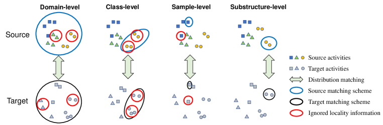
Figure 1: Comparison of different distribution matching schemes in domain adaptation.

For CDAR problems, we argue that these methods can suffer from the under-adaptation and over-adaptation issues since they may ignore the locality information contained in activity data. The locality refers to the fine-grained similarity between two sensor signals that should be considered for domain adaptation. As shown in Figure 1, domain-level matching completely ignores the intra-domain data structure while class-level matching takes a slightly finer alignment (Wang et al., 2018a). However, we find that there exist two un-adapted clusters in activity 2 which means rough matching may result in under-adaptation, i.e., domain- and class-level matching fails to capture the locality information. On the other hand, it is obvious that sample-level methods may be seriously affected by some bad points, such as noisy points or outliers, resulting in over-adaptation, i.e., sample-level matching suffers from overfitting when learning the locality information. In addition, sample-level methods need to match too many points, which is notoriously time-consuming.

In this paper, we tackle domain adaptation based HAR from a different perspective, and hence propose Substructural Domain Adaptation (SSDA) for accurate and robust domain adaptation. Generally speaking, Substructure describes the fine-grained latent distribution of data. For the entire class, it can be understood as a data cluster of the class. Figure 1 shows how SSDA performs substructure-level matching. Compared with the domain- and class-level methods, SSDA utilizes more fine-grained locality information to overcome under-adaptation. In contrast to sample-level methods that can be easily affected by noise or outliers, SSDA utilizes the substructure of the data that can prevent over-adaptation. Based on SSDA, we propose an optimal transport-based implementation, namely, Substructural Optimal Transport (SOT), for the cross-domain HAR problems. OT (Villani, 2008) has a solid theoretical background and allows a flexible mapping without being restricted to a particular hypothesis class (Redko et al., 2017), hence it has no restriction on the numbers of substructures in different domains. Specifically, SOT first obtains the internal substructures by a clustering method. Then, the activity substructure weights of the source domain are given via partial optimal transport according to its distance from the target domain. Finally, two representations of substructures are used to learn a transportation plan matching the probability distribution functions (PDFs) on both substructures. We conduct experiments on four public activity recognition datasets (UCI DSADS (Barshan & Yüksek, 2014), UCI-HAR (Anguita et al., 2012), USC-HAD (Zhang & Sawchuk, 2012), and PAMAP2 (Reiss & Stricker, 2012)). The results demonstrate that our method outperforms other state-of-the-art methods with a significant improvement of over $\mathbf{9}\%$ w.r.t classification accuracy, while it is $\mathbf{5}\times$ faster than traditional OT-based DA methods with the same hyper-parameters.

Our contributions are mainly three-fold:

1. We propose SSDA for accurate and robust domain adaptation. SSDA can overcome the under-adaptation and over-adaptation issues in existing domain-, class-, or sample-level matching methods.

2. Based on SSDA, we propose an optimal transport-based implementation, SOT, to perform cross-domain activity recognition.

3. Comprehensive experiments on four public activity recognition datasets demonstrate the superiority of SOT ($\mathbf{9}\%+$ improvement in accuracy). In addition, SOT is $\mathbf{5}\times$ faster than traditional OT-based DA methods with the same hyper-parameters.

2 Related Work

2.1 Human Activity Recognition

Human activity recognition has been a popular research topic in ubiquitous computing for its important role in human daily life. HAR attempts to identify and analyze human activities using learned high-level knowledge from raw data of various types of sensors. Several surveys have summarized recent progress in HAR. (Bux et al., 2017; Beddiar et al., 2020) summed up vision-based HAR and (Wang et al., 2019; Dang et al., 2020) summarized recent work from a different point. In this paper, we focus on work about sensor-based HAR.

Conventional machine learning approaches often treat HAR as a standard time series classification problem. After getting raw data from sensors, they first preprocess the raw data which includes denoising (Castro et al., 2016) and segmentation (Triboan et al., 2019). Then feature extraction and feature selection (Dawn & Shaikh, 2016) are implemented to extract useful features from the pre-processed data. In the following, different models, such as random forest (RF) (Hu et al., 2018), Bayesian networks (Xiao & Song, 2018), and support vector machine (SVM) (Reyes-Ortiz et al., 2016; Chen & Wang, 2018), are built with selected features. Finally, we can use these learned models to make activity inferences. Deep learning based HAR (Ignatov, 2018; Zhao et al., 2018b; Khan & Taati, 2017; Hassan et al., 2018a; b) automatically extracts abstract features through several hidden layers and reduces the effort of choosing the right features.

However, most of the methods mentioned before assume that the training and testing data are in the same distribution, which is not suitable for CDAR problems. As for CDAR problems, source and target data are usually from a different distribution, which results in weak generalization of the aforementioned methods. Therefore, approaches to the CDAR are needed. And in this paper, we mainly focus on the traditional approaches for CDAR problems.

2.2 Transfer Learning and Domain Adaptation

Transfer learning tries to leverage source domain knowledge to help learn models in the target domain, which mitigates the problem that the target domain has no label or few labels. (Pan & Yang, 2009; Weiss et al., 2016) concluded the traditional transfer learning methods, and (Tan et al., 2018; Wilson & Cook, 2020) introduced the deep transfer learning methods. Domain adaptation, as a branch of the transfer learning, solves the problem that a distribution shift exists between different domains and has been successfully applied in many applications, such as visual image classification (Wang & Deng, 2018), natural language processing (Li et al., 2020), sentiment classification (Dai et al., 2020), etc. We roughly divide domain adaptation into two categories: 1) rough matching which includes domain-level matching, class-level matching, and both domain- and class-level matching; 2) sample-level matching which is a meticulous matching way.

Domain adaptation has developed for many years and most of those methods exploit rough matching between two domains. (Pan et al., 2010) proposed a method, named Transfer Component Analysis (TCA), which learns a kernel in the reproducing kernel Hilbert space (RKHS) to minimize the maximum mean discrepancy (MMD) between domains. (Wang et al., 2018a) proposed stratified transfer learning (STL) and achieved the goal of intra-class transfer. Joint distribution adaptation (JDA) (Long et al., 2013) is based on minimizing joint distribution between domains. (Wang et al., 2017; 2020) extended it and proposed Balanced Distribution Adaptation (BDA) which adaptively adjusts the importance of marginal distribution and conditional distribution. (Zhao et al., 2020) proposed a method, named Local Domain Adaptation (LDA), which takes a compromise between domain- and class-level matching and utilizes high-level abstract clusters to organize data.

Sample-level matching is the other way to match distribution between domains and the representative work is (Courty et al., 2016). Nicolas Courty et al. utilized the theory of optimal transport to learn the coupling between two probability density functions. Through the barycentric mapping (Villani, 2008), the images of the source samples in the target domain are obtained, and then a simple classification model can be used to classify the target samples. (Kerdoncuff et al., 2020) extended it which designs a metric learning optimal transport (MLOT) algorithm to optimizes a mahalanobis distance. Besides optimal transport based methods, (Das & Lee, 2018b; a) used hypergraph matching to match the samples between two domains.

SSDA is different from these methods. It takes advantage of the substructure of domains and utilizes the substructure-level matching to seek the balance of rough matching and sample-level matching.

2.3 Human Activity Recognition with Transfer Learning

There is much prior work focusing on HAR with transfer learning and a detailed survey can be found in (Cook et al., 2013).

(Zhao et al., 2011) proposed an algorithm known as transfer learning embedded decision tree (TransEMDT) which integrates a decision tree and the k-means clustering algorithm to solve the cross-people activity recognition problem. Lin et al. (Lin et al., 2016) identified a compact joint subspace for each class and then measured the distance between classes using principal angle. (Wang et al., 2018a) tried to learn more reliable pseudo labels using the majority voting technique on both domains. (Rey & Lukowicz, 2017) considered a special case that the new domain just contains the old one and (Feuz & Cook, 2017) proposed a heterogeneous transfer learning method for HAR. Recently, Qin et al. (Qin et al., 2019) proposed an adaptive spatial-temporal transfer learning (ASTTL) approach to select the most similar source domain to the target domain and accurately transfer activity. Despite many approaches have been designed to solve the CDAR problem and some of them attempted to use clustering methods, little work is substructure-based. SOT tries to complete substructure-level matching through joint Gaussian Mixture Model and optimal transport. The number of substructures may be different from the number of the classes.

3 Method

3.1 Problem Formulation

In a CDAR problem (Wang et al., 2018a), a labeled source domain $\mathcal{D}_{s}=\{(\mathbf{x}_{i},y_{i})\}_{i=1}^{n_{s}}$ and an unlabeled target domain $\mathcal{D}_{t}=\{\mathbf{x}_{j}\}_{j=1}^{n_{t}}$ are given, where $n_{s}$ and $n_{t}$ are the number of source and target samples respectively. In our problem, $\mathcal{D}_{s}$ and $\mathcal{D}_{t}$ have the same feature spaces and label spaces, i.e. $\mathcal{X}_{s}=\mathcal{X}_{t}\subset\mathbb{R}^{d}$ and $\mathcal{Y}_{s}=\mathcal{Y}_{t}$, where $d$ is the feature dimension. $y_{s},y_{t}\in\{1,\cdots,C\}$, and $C$ is the number of classes. Two domains have different distributions, i.e., $p_{s}(\mathbf{x},y)\neq p_{t}(\mathbf{x},y)$. The goal of cross-domain learning is to obtain the labels $y_{t}$ for the target domain with the help of the source domain $\mathcal{D}_{s}$.

3.2 Motivation

In a CDAR problem, labeled source data often has a different distribution with target data. For example, source data may be collected from the sensor tied on the front right hip while target data may contain waist-mounted smartphone data. When we perform rough distribution matching which aligns whole data or aligns data based on classes, we may not be able to match data perfectly since different people have their styles even performing the same activity. Thus, we need to capture the locality information.

The raw activity data can be represented as $\mathbf{x}=\mathbf{z}+\bm{\delta}$, where $\mathbf{z}\in\mathbb{R}^{d}$ represents an activity prototype containing the data collected from the standard activity in an ideal situation and $\bm{\delta}$ corresponds to the noise in reality. Therefore, sample-level matching that aligns $\mathbf{x}$ directly may introduce noise, and performing sample-level matching might have no practical meaning. Overall, a compromise between rough matching and sample-level matching is needed to obtain more fine-grained alignments and avoid noise influence.

Apart from empirical analysis, we theoretically analyze our motivation by formulating the distribution as:

$$p(\mathbf{x}) =\sum_{y}p(\mathbf{x}|y)p(y)$$ (1a)

$$=\sum_{y}(\sum_{o}p(\mathbf{x},o|y))p(y)$$

$$=\sum_{y}\sum_{o}p(\mathbf{x}|y,o)p(y,o)\text{~{}(For source domain)}$$ (1b)

$$=\sum_{o}\sum_{y}p(\mathbf{x}|y,o)p(y|o)p(o)$$

$$=\sum_{o}p(\mathbf{x}|o)p(o).\text{~{}(For target domain)}$$ (1c)

According to Equation equation 1a, domain-level matching tries to match $p(\mathbf{x})$ while class-level matching tries to match $p(\mathbf{x}|y)$. From the previous analysis, we know that one class may include more fine-grained locality information, which means class-level matching may not be enough. Therefore, a deeper decomposition of $\mathbf{x}$ is needed. We denote $o$ as the locality information contained in each $y$, i.e., $o$ is the substructure. As shown in Equation equation 1b, we can divide the labeled source domain into multiple substructures. Since the target domain has no labels, further conversion is performed and Equation equation 1c shows we can divide the target domain into finer substructures.

We know that

$$p(y|o)=\begin{cases}1&o\mathrm{~{}~{}is~{}~{}part~{}~{}of~{}~{}}y\\ 0&o.w.\\ \end{cases}$$ (2)

Denote the substructure of $o$ as $y_{o}$, then $\sum_{y}\sum_{o}p(\mathbf{x}|y,o)p(y,o)=\sum_{o}p(\mathbf{x},y_{o}|o)p(o)$, which indicates that Equation equation 1b and Equation equation 1c are identical. Now, we can match $p(\mathbf{x}|o)$. Obviously, this substructure-level matching is more fine-grained compared with domain- and class-level matching while it avoids the influence of noise via the use of substructures compared with sample-level matching.

Table 1 compares different matching schemes.

Table 1: Comparison between different matching schemes.

Type	Assumption	Formulation	Limitations
Domain-level	domain-invariant features	$p(\mathbf{x}_{s})\longleftrightarrow p(\mathbf{x}_{t})$	too coarse matching
Class-level	class-invariant features	$p(\mathbf{x}_{s}|y_{s})\longleftrightarrow p(\mathbf{x}_{t}|y_{t})$	coarse matching
Substructure-level	substructure-invariant features	$p(\mathbf{x}_{s},y_{s}|o_{s})\longleftrightarrow p(\mathbf{x}_{t}|o_{t})$
Sample-level	no strict restrictions	$(\mathbf{x}_{s},y_{s})\longleftrightarrow\mathbf{x}_{t}$	affected by noise, low-efficiency

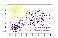
(a) toy dataset distribuion

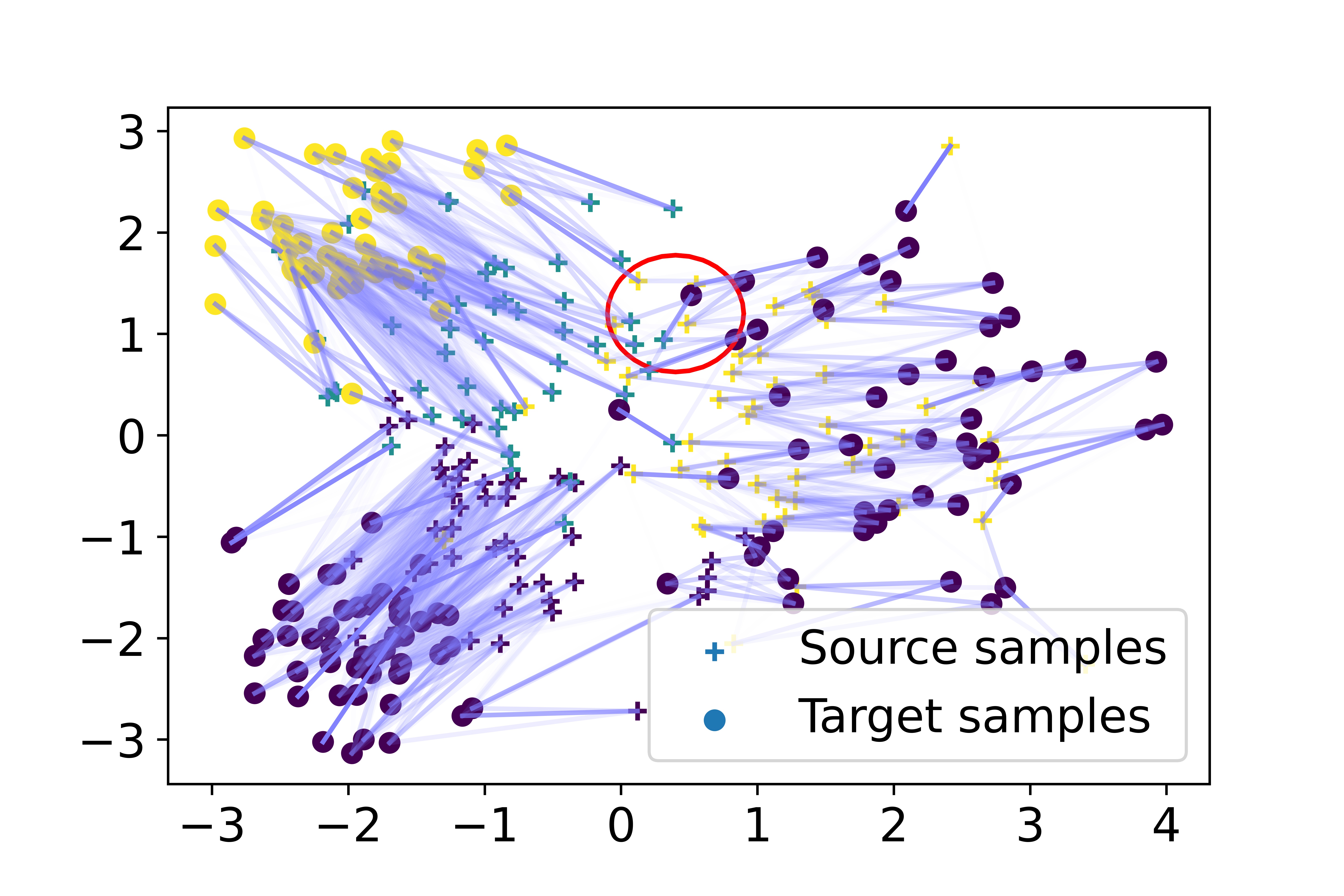
(b) OTDA for toy dataset

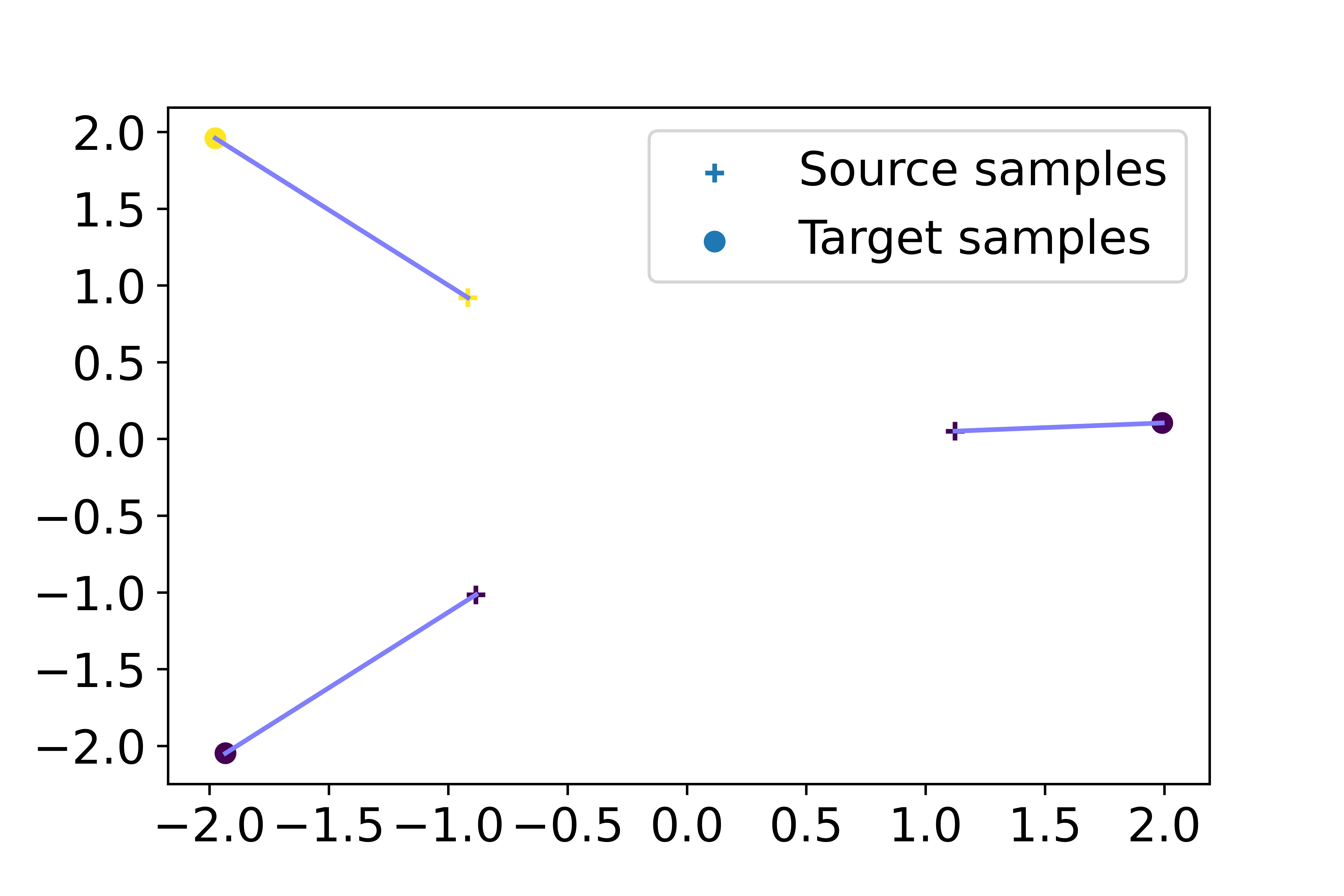
(c) SOT for toy dataset

Figure 2: Toy example to show the effectiveness of substructure-level matching.

To explain the necessity of using the substructures more clearly, we give a toy example. As we can see from Figure 2(a), the source has three clusters that are sampled from a Gaussian Mixture Model (GMM) and the target also has three clusters sampled from a slightly different GMM. Both domains have two classes while the different colors respond to the different classes. It is obvious that one of the classes has two components, which means rough matching may not be suitable. Next, we consider the sample-level matching. The concrete data can be treated as the noisy version of the prototypes, i.e. the cluster centers adding perturbation. Figure 2(b) shows that if we directly match two domains with concrete data points, there will be miss matching. The red circle in Figure 2(b) points one miss matching. Intuitively speaking, the matching of noise points to noise points has no practical meaning.

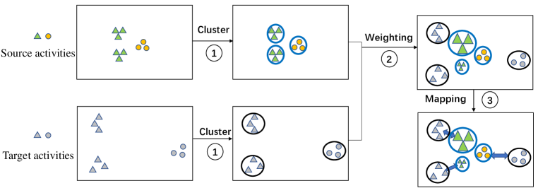
Figure 3: Overview of the SSDA framework.

3.3 SSDA: A general framework for domain adaptation

In this paper, we propose a general Substructural Domain Adaptation (SSDA) method. SSDA is a general framework consistent with the substructure and Figure 3 illustrates the main process of SSDA which mainly contains three steps. Firstly, SSDA clusters the data to obtain the substructures of activities. As a general framework, we can choose a suitable clustering algorithm for customization. Then, it gives weights to the source substructures according to priors or adaptive methods. Weight represents the importance of substructures and different substructures often play different roles. For example, some substructures far away from most data should play small roles with small weights. For simplicity, we usually give uniform weights to all structures without priors. Finally, mapping is performed on the substructures of different domains. We can extend some traditional method, such as CORrelation alignment (CORAL) (Sun et al., 2016), to perform substructure-level matching, which is really commendable.

3.4 SOT: an OT implementation of SSDA

In this section, we propose an OT implementation of SSDA, named SOT. SOT utilizes GMM to get substructures while it uses OT to perform weighting and mapping. According to the substructure representation, we introduce $\mathrm{SOT}_{c}$ with center representation and $\mathrm{SOT}_{g}$ with distribution representation.

3.4.1 Substructures Generation And Representations

We denote $\bm{\delta}\sim\mathcal{N}(0;\bm{\sigma}^{2})$ and $\mathbf{X}$ represents all feature data. Equivalently, $\mathbf{X}_{k}$ conforms to a Gaussian distribution whose center is the corresponding prototypes, i.e. $\mathbf{X}_{k}\sim\mathcal{N}(\mathbf{z}_{k},\bm{\sigma}_{k})$. $\mathbf{z}_{k}$ means the value of $k$th center, $\bm{\sigma}_{k}$ means the $k$th covariance, and $\mathbf{X}_{k}$ means the data belong to the $k$th cluster. Now, we have data $\mathbf{X}$ and our goal is to get $\mathbf{z}_{k}$ and $\bm{\sigma}_{k}$. It is easy to use Expectation Maximum (EM) (Dempster et al., 1977) algorithm to obtain the parameters of the Gaussian Mixture Models.

To maintain label consistency in the source domain, we treat the source domains as a mixture distribution of $C$ Gaussian mixture models and each one corresponds to one class in the source domain. The number of components is determined by the Bayesian Information Criterion (BIC) (Schwarz et al., 1978), i.e.

$$BIC=-2\ln(L)+k\ln(m),$$ (3)

where $L$ represents the maximized value of the likelihood function for the estimated model, $k$ represents the number of free parameters to be estimated, and $m$ is the sample size. We seek $K$ which minimizes BIC. Due to the lack of labels in the target domain, we have to perform clustering on the entire target domain and the number of clusters is up to the specific dataset.

After getting the clusters in the source domain and the target domain, we design two different ways to represent the substructures which correspond to $\mathrm{SOT}_{c}$ and $\mathrm{SOT}_{g}$ respectively. $\mathrm{SOT}_{c}$ with center representation utilizes only information from cluster center, and it is simple and computationally efficient while $\mathrm{SOT}_{g}$ with distribution considers more information on clusters, but it needs some approximations when computing.

$\mathrm{SOT}_{c}$: After clustering, two domains are expressed as the cluster centers, i.e. $\mu_{c,s}=\sum_{i=1}^{k_{s}}w_{s,i}\delta_{\mathbf{z}_{s,i}},\mu_{c,t}=\sum_{i=1}^{k_{t}}w_{t,i}\delta_{\mathbf{z}_{t,i}}$. $\mathbf{z}\in\mathbb{R}^{d}$ represents the cluster centers and $\delta_{\mathbf{z}}$ is a Dirac function at location $\mathbf{z}$. $\mu_{c,s},\mu_{c,t}$ are distributions of the source domain and the target domain respectively and $w$ are probability masses associated to the $\mathbf{z}$. Obviously, $\sum_{i=1}^{k_{s}}w_{s,i}=1,\sum_{i=1}^{k_{t}}w_{t,i}=1$. In addition, the squared Euclidean distance can be chosen as the cost between $\mathbf{z}_{s,i}$ and $\mathbf{z}_{t,j}$, i.e.

$$c(\mathbf{z}_{s,i},\mathbf{z}_{t,j})=||\mathbf{z}_{s,i}-\mathbf{z}_{t,j}||_{2}^{2}.$$ (4)

$\mathrm{SOT}_{g}$: This one utilizes the cluster distributions to represent the substructures, and the covariance of the clusters can be understood as the difficulty of the activity for the person. Therefore, the source domain can be expressed as $\mu_{g,s}=\sum_{i=1}^{k_{s}}w_{s,i}\mathcal{N}(\mathbf{z}_{s,i},\bm{\sigma}_{s,i})$ and the target domain can be expressed as $\mu_{g,t}=\sum_{i=1}^{k_{t}}w_{t,i}\mathcal{N}(\mathbf{z}_{t,i},\bm{\sigma}_{t,i})$. The meanings of the symbols are similar to the first way. The only difference is that we use a Gaussian distribution $\mathcal{N}(\mathbf{z},\bm{\sigma})$ instead of a Dirac function $\delta_{\mathbf{z}}$. In this situation, the squared Wasserstein distance (Peyré et al., 2019) replaces the squared Euclidean distance as the cost function, i.e.

$$c(\mathcal{N}(\mathbf{z}_{s,i},\bm{\sigma}_{s,i}),\mathcal{N}(\mathbf{z}_{t,j},\bm{\sigma}_{t,j})) =W_{2}^{2}(\mathcal{N}(\mathbf{z}_{s,i},\bm{\sigma}_{s,i}),\mathcal{N}(\mathbf{z}_{t,j},\bm{\sigma}_{t,j}))$$

$$=||\mathbf{z}_{s,i}-\mathbf{z}_{t,j}||^{2}+B(\bm{\sigma}_{s,i},\bm{\sigma}_{t,j})^{2},$$

where $B$ is the Bures metric (Bhatia et al., 2019) between positive definite matrices and can be calculated as follows,

$$B(\bm{\sigma}_{s,i},\bm{\sigma}_{t,j})^{2}=tr(\bm{\sigma}_{s,i}+\bm{\sigma}_{t,j}-2(\bm{\sigma}_{s,i}^{1/2}\bm{\sigma}_{t,j}\bm{\sigma}_{s,i}^{1/2})^{1/2}),$$ (5)

where $tr(\cdot)$ denotes the trace of a matrix, $\bm{\sigma}^{1/2}$ is the matrix square root. For simplicity, we force the covariance matrix to be a diagonal matrix, i.e. $\bm{\sigma}=diag(r_{i})_{i=1}^{d}$. In this case, the Bures metric is the Hellinger distance $B(\bm{\sigma}_{s,i},\bm{\sigma}_{t,j})=||\sqrt{\mathbf{r}_{s,i}}-\sqrt{\mathbf{r}_{t,j}}||$. Overall, the cost function is

$$c(\mathcal{N}(\mathbf{z}_{s,i},\bm{\sigma}_{s,i}),\mathcal{N}(\mathbf{z}_{t,j},\bm{\sigma}_{t,j})) =||\mathbf{z}_{s,i}-\mathbf{z}_{t,j}||^{2}+||\sqrt{\mathbf{r}_{s,i}}-\sqrt{\mathbf{r}_{t,j}}||_{2}^{2}$$ (6)

$$=||(\mathbf{z}_{s,i},\sqrt{\mathbf{r}_{s,i}})-(\mathbf{z}_{t,j},\sqrt{\mathbf{r}_{t,j}})||_{2}^{2}.$$

$\mathbf{r}_{s,i}$ and $\mathbf{r}_{t,j}$ represent diagonals of the $i$th source domain cluster’s covariance and the $j$th target domain cluster’s covariance respectively. $(\mathbf{z},\sqrt{\mathbf{r}})$ concatenates the $\mathbf{z}$ and $\sqrt{\mathbf{r}}$ and serves as the new feature of the substructure.

3.4.2 Weighting Source Substructures

For unity, we denote the source domain as $P_{s}=\sum_{i=1}^{k_{s}}w_{s,i}p_{s,i}$ and denotes the target domain as $P_{t}=\sum_{i=1}^{k_{t}}w_{t,i}p_{t,i}$. Due to little information about the target domain, we treat $p_{t,i}$ equally and fix $w_{t,i}$ to $1/k_{t}$. Now, we compute the $w_{s,i}$ adaptively.

Since we only know $\sum_{i=1}^{k_{s}}w_{s,i}=1$, it can be seen as a partial optimal transport problem, and the upper bounds of $w_{s,i}$ are all 1. Obviously, the total cost of the partial optimal transport is $\langle\bm{\pi},\mathbf{C}\rangle_{F}$, where $\langle\cdot,\cdot\rangle_{F}$ is the Frobenius dot product, $\mathbf{C}$ is the cost matrix, and $\bm{\pi}$ is the coupling matrix between two PDFs. For calculation convenience, an entropy item, i.e.$H(\bm{\pi})=\sum_{ij}\pi_{ij}\log\pi_{ij}$, is added. Now, our goal is to obtain the optimal transport.

$$\bm{\pi}^{*}_{1} = \arg\min_{\bm{\pi}}\langle\bm{\pi},\mathbf{C}\rangle_{F}+\lambda_{1}H(\bm{\pi})$$ (7)

$$s.t \bm{\pi}^{T}\mathbf{1}_{k_{s}}=\mathbf{w}_{t}$$

$$\bm{\pi}\mathbf{1}_{k_{t}}\leq\mathbf{1}_{k_{s}}$$

$$\mathbf{1}_{k_{t}}^{T}\bm{\pi}^{T}\mathbf{1}_{k_{s}}=1.$$

$\mathbf{1}_{k}$ is k-dimensional vector of ones and $\lambda_{1}$ is a hyper-parameter that balances the calculation speed and accuracy. $H(\bm{\pi})$ requires $\bm{\pi}\geq 0$. When $\bm{\pi}\geq 0$ and $\mathbf{1}_{k_{t}}^{T}\bm{\pi}^{T}\mathbf{1}_{k_{s}}=1$, it is obvious that $\bm{\pi}\mathbf{1}_{k_{t}}\leq\mathbf{1}_{k_{s}}$ always holds. In addition, $\mathbf{1}^{T}_{k_{t}}\mathbf{w}_{t}=1$ holds, which means $\mathbf{1}_{k_{t}}^{T}\bm{\pi}^{T}\mathbf{1}_{k_{s}}=1$ also always holds. Therefore, Equation equation 7 can be simplified as the following.

$$\bm{\pi}^{*}_{1} = \arg\min_{\bm{\pi}}\langle\bm{\pi},\mathbf{C}\rangle_{F}+\lambda_{1}H(\bm{\pi})$$ (8)

$$s.t \bm{\pi}^{T}\mathbf{1}_{k_{s}}=\mathbf{w}_{t}.$$

We denote the feasible solution set of $\bm{\pi}^{T}\mathbf{1}_{k_{s}}=\mathbf{w}_{t}$ as $C_{1}$. Obviously, the $C_{1}$ is a convex set. The optimization goal of Equation equation 8 is also convex. And, it is easy to get the closed form of this problem. In the following, the Lagrange method is adopted to solve the problem.

We denote $\bm{\phi}$ as the Lagrange multiplier, then our goal can be derived as

$$L=\langle\bm{\pi},\mathbf{C}\rangle_{F}+\lambda_{1}H(\bm{\pi})+\bm{\phi}^{T}(\bm{\pi}^{T}\mathbf{1}_{k_{s}}-\mathbf{w}_{t}).$$

To get the optimal point, the following equations must hold:

$$\frac{\partial L}{\partial\bm{\pi}}=0$$ (9a)

$$\bm{\pi}^{T}\mathbf{1}_{k_{s}}-\mathbf{w}_{t}=\mathbf{0}.$$ (9b)

Using Equation equation 9a, we can get $\mathbf{C}+\lambda_{1}(1+\log\bm{\pi})+\mathbf{1}_{k_{s}}\bm{\phi}^{T}=\mathbf{0},$ which means

$$\bm{\pi}=e^{-\frac{\mathbf{1}_{k_{s}}\bm{\phi}^{T}-\mathbf{C}}{\lambda_{1}}-1}.$$ (10)

Then, we substitute Equation equation 10 into Equation equation 9b and get

$${e^{\frac{-\mathbf{1}_{k_{s}}\bm{\phi}^{T}-\mathbf{C}}{\lambda_{1}}-1}}^{T}\mathbf{1}_{k_{s}}=\mathbf{w}_{t}.$$

Therefore, we get

$${e^{\frac{-\mathbf{C}}{\lambda_{1}}-1}}^{T}\odot{e^{\frac{-\mathbf{1}_{k_{s}}\bm{\phi}^{T}}{\lambda_{1}}}}^{T}\mathbf{1}_{k_{s}}=\mathbf{w}_{t},$$

where $\odot$ means element-wise product. Obviously, each element in the same row of $\exp(\frac{-\mathbf{1}_{k_{s}}\bm{\phi}^{T}}{\lambda_{1}})$ is the same number, and we can easily get the optimal $\bm{\pi}^{*}$. We initialize $\bm{\pi}_{0}=\exp(-\frac{\mathbf{C}}{\lambda_{1}}-1)$ and get

$$\bm{\pi}^{*}_{1}=\bm{\pi}_{0}\mathrm{diag}(\mathbf{w}_{t}\oslash\bm{\pi}_{0}^{T}\mathbf{1}_{k_{s}}),$$ (11)

where $\oslash$ denotes element-wise divide and $\mathrm{diag}$ denotes diagonals. Once the optimal coupling matrix $\bm{\pi}^{*}_{1}$ is obtained, the source weight can be easily calculated as $\mathbf{w}_{s}=\bm{\pi}^{*}_{1}\mathbf{1}_{k_{t}}$.

3.4.3 OT-based Mapping of the Substructures

Through the previous steps, the source domain distribution is $P_{s}=\sum_{i=1}^{k_{s}}w_{s,i}p_{s,i}$ while the target domain distribution is $P_{t}=\sum_{i=1}^{k_{t}}w_{t,i}p_{t,i}$. And the label corresponding to $p_{s,i}$ is the label of the data belongs to $i$th cluster in the source domain, i.e. $\tilde{y}_{s,i}$. According to Equation equation 4 or Equation equation 6, we can easily get the cost matrix $\mathbf{C}$. Following (Courty et al., 2016), the objective for SOT is

$$\bm{\pi}^{*} = \arg\min_{\bm{\pi}}\langle\bm{\pi},\mathbf{C}\rangle_{F}+\lambda H(\bm{\pi})+\eta\Omega(\bm{\pi})$$ (12)

$$s.t \bm{\pi}^{T}\mathbf{1}_{k_{s}}=\mathbf{w}_{t}$$

$$\bm{\pi}\mathbf{1}_{k_{t}}=\mathbf{w}_{s}.$$

$\Omega(\bm{\pi})$ is group-sparse regularizer, and it expects that each target sample receives masses only from source samples that have the same label. And following (Courty et al., 2016), we define the regularizer as $\Omega(\bm{\pi})=\sum_{j}\sum_{cl}||\bm{\pi}(I_{cl},j)||_{2}$, where $||\cdot||_{2}$ denotes the $l_{2}$ norm and $I_{cl}$ contains the indices of rows in $\bm{\pi}$ related to source domain samples of class $cl$. $\bm{\pi}(I_{cl},j)$ is a vector containing coefficients of the $j$th column of $\bm{\pi}$ associated to class $cl$, and it induces the desired sparse representation in the target samples. $\lambda$ and $\eta$ are hyper-parameters. We use generalized conditional gradient (GCG) following (Courty et al., 2016) to solve the optimization problem.

Once obtaining the optimal coupling matrix $\bm{\pi}^{*}$, we can compute the transformation of $\mathbf{p}_{s,i}$ by barycentric mapping, i.e. $\hat{\mathbf{p}}_{s,i}=\arg\min_{\mathbf{p}}\sum_{j}\pi^{*}(i,j)c\left(\mathbf{p},\mathbf{p}_{t,j}\right)$. When the cost function is the squared $l_{2}$ distance, this barycentric mapping can be expressed as:

$$\hat{\mathbf{P}}_{s}=diag(\bm{\pi}^{*}\mathbf{1}_{k_{t}})^{-1}\bm{\pi}^{*}\mathbf{P}_{t},$$ (13)

where $\mathbf{P}_{t}$ represents the target representation and $\hat{\mathbf{P}}_{s}$ represents the source mapping representation. Now, any traditional machine learning model, such as 1-Nearest Neighbor (1NN), can be used to learn the predictions with help of $\hat{\mathbf{P}}_{s}$ and $\tilde{y}_{s,i}$. After getting the label $\tilde{y}_{t,i}$ corresponding to $p_{t,i}$, we assign the same label, $\tilde{y}_{t,i}$, to the data belonging to $p_{t,i}$ in the target domain.

The overall process of SOT is described in Algorithm 1.

Algorithm 1 SOT: Substructural Optimal Transport

Input: source dataset $\mathcal{D}_{s}=\{(\mathbf{x}_{s,i},y_{s,i})\}_{i=1}^{n_{s}}$, target dataset $\mathcal{D}_{t}=\{(\mathbf{x}_{t,i})\}_{i=1}^{n_{t}}$, hyper-parameters $\lambda_{1},\lambda,\eta,k_{t}$
  Output: target labels$\{y_{t,i}\}_{i=1}^{n_{t}}$

1:Use EM for GMM, cluster each class data in the source domain to obtain $\{(\mathbf{p}_{s,i},\tilde{y}_{s,i})\}_{i=1}^{k_{s}}$. The number of clusters is determined by Equation equation 3.

2:Use EM for GMM to obtain $\{(\mathbf{p}_{t,i})\}_{i=1}^{k_{t}}$

3:Compute cost matrix $\mathbf{C}$ according Equation equation 4 ($\mathrm{SOT}_{c}$) or Equation equation 6 ($\mathrm{SOT}_{g}$)

4:Use Equation equation 11 to compute the source substructures’ weights $\mathbf{w}_{s}$. Set $\mathbf{w}_{t}=\frac{\mathbf{1}_{k_{t}}}{k_{t}}$

5:Use GCG to compute the optimal coupling matrix $\bm{\pi}^{*}$

6:According to Equation equation 13, compute the transformation of the source substructures and obtain $\hat{\mathbf{P}_{s}}$

7:Use $\hat{\mathbf{P}}_{s}$ and $\tilde{\mathbf{Y}}_{s}$ to build the model and predict the $\mathbf{P}_{t}$. The predictions are noted as $\tilde{\mathbf{Y}}_{t}$

8:Assign $\tilde{y}_{t,i}$ to the data belonging to $p_{t,i}$ in the target domain

4 Experimental Evaluation

In this section, we evaluate the performance of SOT via extensive experiments on cross-domain activity recognition. The source code of our SOT is at https://github.com/jindongwang/transferlearning/tree/master/code/traditional/sot.

4.1 Dataset and Preprocessing

We adopt four common public datasets. Table 2 describes the information and the selected data volume of these datasets. In the following, we briefly introduce the basic information of each dataset, and more information can be found in their original papers.

UCI daily and sports dataset (DSADS, D) (Barshan & Yüksek, 2014) consists of 19 activities collected from 8 subjects wearing body-worn sensors on 5 body parts. UCI human activity recognition using smartphones data set (UCI-HAR, H) (Anguita et al., 2012) is collected by 30 subjects performing 6 daily living activities with a waist-mounted smartphone. USC-SIPI human activity dataset (USC-HAD, U) (Zhang & Sawchuk, 2012) composes of 9 subjects executing 12 activities with a sensor tied on the front right hip. PAMAP2 physical activity monitoring dataset (PAMAP2, P) (Reiss & Stricker, 2012) contains data of 18 different physical activities, performed by 9 subjects wearing 3 sensors.

Table 2: Information of four datasets. Num means the select data volume.

Dataset	Subject	Activity	Sample	Location	Num
DSADS	8	19	1.14M	Tarso, Right Arm, Left Arm, Right Leg, Left Leg	2400
UCI-HAR	30	6	1.31M	Waist	6616
USC-HAD	14	12	2.81M	Front Right Hip	4187
PAMAP	9	18	2.84M	Wrist, Chest, Ankle	1688

The cross-domain activity recognition experimental setup is in the following ways. Since different datasets use different sensors and contain different classes of activities, we need to unify our experimental setup for datasets first, and we choose the common parts of the sensors and four common categories of activities. Specifically, we utilize the accelerometer and gyroscope, and each sensor provides 3-axial data (x-, y- and z-axis). We combine them by $\alpha=\sqrt{x^{2}+y^{2}+z^{2}}$ following (Wang et al., 2018a). Then, according to (Wang et al., 2018a), we exploit the sliding window technique to extract features, and 19 features from both time and frequency domains are extracted for a single sensor. We extract 38 features from one position since two sensors are selected. We choose data from Right Arm, Waist, Front Right Hip, and Right Wrist from these four datasets respectively, and choose four categories, including lying, walking, ascending, descending. In experiments, we perform unsupervised domain adaptation on the target domain.

4.2 Comparison Methods and Implementation Details

We adopt nine comparison methods including both general transfer learning and cross-domain HAR areas:

1. Baseline models

   • 1NN: 1-Nearest Neighbor.

   • LMNN: Large margin nearest neighbor (Weinberger & Saul, 2009).

2. Rough matching

   • TCA: Transfer component analysis (Pan et al., 2010).

   • SA: Subspace alignment (Fernando et al., 2013).

   • CORAL: CORrelation alignment (Sun et al., 2016).

   • STL: Stratified transfer learning (Wang et al., 2018a).

3. Sample-level matching

   • OT: Optimal transport (Cuturi, 2013).

   • OTDA: Optimal transport for domain adaptation (Courty et al., 2016).

   • MLOT: Metric learning optimal transport (Kerdoncuff et al., 2020).

1NN and LMNN serve as baseline models and TCA, SA, and CORAL perform the rough matching while OT, OTDA, and MLOT belong to sample-level matching methods. And all of these methods use a 1NN classifier for the classification tasks. We conduct experiments in every pair of four datasets and construct 12 tasks in total.

For most of the comparison methods, we use the codes from (Wang et al., ) for implementation. For a particular hyper-parameter configuration, we follow the similar protocol used in (Courty et al., 2016). The target domain is partitioned in validation and test sets. The validation set is used to obtain the best accuracy in the range of the possible hyper-parameters. The hyper-parameter range used follows (Kerdoncuff et al., 2020) and we slightly reduce the range to fit our task. With the best selected hyper-parameters, we evaluate the performance on the testing set. Classification accuracy on the target domain is adopted as the evaluation metric.

4.3 Classification Results

Table 3: Activity recognition results on 12 cross-domain tasks.

method	D$\rightarrow$H	D$\rightarrow$U	D$\rightarrow$P	H$\rightarrow$D	H$\rightarrow$U	H$\rightarrow$P	U$\rightarrow$D	U$\rightarrow$H	U$\rightarrow$P	P$\rightarrow$D	P$\rightarrow$H	P$\rightarrow$U	AVG
NA	62.70	56.40	66.03	65.16	55.03	60.81	71.30	61.38	60.37	60.99	55.26	51.63	60.59
LMNN	55.24	65.74	48.38	64.27	56.55	65.00	64.58	65.46	67.13	59.53	39.11	41.21	57.68
TCA	60.79	51.98	65.66	62.50	41.87	52.06	69.06	53.43	60.88	57.81	46.38	51.45	56.16
SA	63.61	57.36	65.44	66.35	55.60	60.88	70.62	59.64	61.18	62.60	55.45	50.58	60.78
CORAL	64.23	52.25	64.85	64.48	53.03	64.41	68.75	61.93	60.15	60.21	56.20	54.46	60.41
STL	62.83	70.93	65.66	66.15	65.89	67.43	74.69	68.76	65.00	68.96	56.75	55.27	65.69
OT	62.13	65.86	65.66	68.91	58.58	67.50	69.90	59.49	63.75	66.77	51.71	57.59	63.15
OTDA	59.36	54.97	65.52	68.91	59.45	67.50	70.26	62.25	63.09	67.19	53.41	59.09	62.58
MLOT	62.53	53.33	64.85	68.12	58.10	62.13	69.53	59.68	61.25	65.99	63.30	49.24	61.51
$\mathrm{SOT}_{c}$	67.74	79.74	73.31	73.39	70.87	73.23	80.99	78.04	74.41	76.46	72.82	76.51	74.79
$\mathrm{SOT}_{g}$	74.84	79.74	68.68	73.39	71.26	73.23	79.90	72.82	72.28	74.48	72.82	76.51	74.16

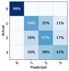
(a) OTDA

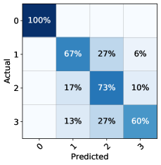
(b) $\mathrm{SOT}_{c}$

Figure 4: Confusion matrices for $U\rightarrow D$.

The results of classification are shown in Table 3 and Figure 4. From these results, we have the following observations: 1) Both $\mathrm{SOT}_{c}$ and $\mathrm{SOT}_{g}$ achieve the best classification accuracy on all tasks. It is obvious that SOT significantly outperforms other methods with a remarkable improvement (over $\mathbf{9}\%$ on average). 2) Compared to baseline methods, rough matching methods and sample-level matching methods only have slight improvements due to neglecting the details or introducing much noise. Thus, being too rough or too delicate is not suitable for cross-dataset activity recognition. 3) Figure 4 shows lying is easy to identify correctly while walking, ascending and descending are difficult to classify, which is in line with the intuition and is consistent with Figure 5(a). 4) $\mathrm{SOT}_{g}$ is slightly worse than $\mathrm{SOT}_{c}$. Maybe because $\mathrm{SOT}_{g}$ uses more approximations when computing. In the following experiments, we use $\mathrm{SOT}_{c}$ by default if there is no special instruction.

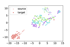
(a) T-SNE for substructures

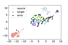
(b) Errors in substructures

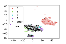
(c) Errors in data

Figure 5: Visualization for $U\rightarrow D$ using SOT. Different colors mean different classes while black means error predictions. The boundaries of different colors correspond to the boundaries of different classes.

4.4 Visualization Study

As we can see in Figure 5(a), the number of points is much smaller after clustering, which can bring high efficiency, and the margins between points are bigger. The class of the substructures in the target domain is temporarily determined by most of the data in the corresponding cluster. In Figure 5(b), we can see that it is easy to misclassify the points which are near the margins or intersected with other classes’ points. Due to the bigger margins and the fewer intersecting points, the accuracy on the substructures is $73\%$ while the accuracy on raw data using OTDA is $70.375\%$. Figure 5(c) shows the misclassified data using $\mathrm{SOT}_{c}$ and the accuracy is improved over $\mathbf{9}\%$ due to the exploitation of the substructures.

4.5 Ablation Study

We first demonstrate SSDA is not limited to its OT implementation (i.e., SOT), but a general framework, and then evaluate the importance and robustness of three important parts of SOT, namely, substructures generation, weighting source substructures and OT-based mapping of substructures.

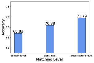
(a) CORAL

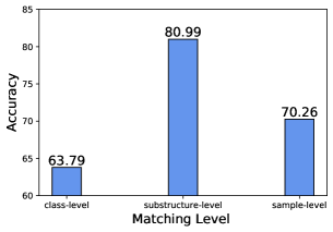
(b) OTDA

Figure 6: Accuracy of different matching levels with different methods for task $U\rightarrow D$.

4.5.1 Implementing SSDA using other methods

We implement CORAL with domain-, class- and substructure-level matching and Figure 6(a) shows that class-level matching CORAL gets better accuracy than domain-level matching while substructure-level matching CORAL achieves the best accuracy, which demonstrates finer matching gets better results. In addition, we implement OTDA with class-, substructure- and sample-level matching, and Figure 6(b) illustrates that substructure-level matching OTDA gets a better accuracy than the sample-level matching OTDA, which may be substructure-level matching is robust to noise. Overall, Figure 6 demonstrates SSDA is a general framework and can achieve commendable results.

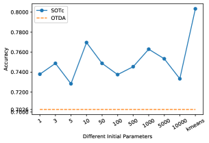
(a) Results for $U\rightarrow D$ using different random params for GMM

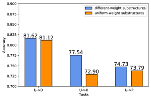
(b) Results for $U\rightarrow D$ using substructures with uniform or different weights

Figure 7: Ablation study of substructures generation and weighting source substructures.

4.5.2 Substructures generation

We generate substructures with GMM using different initial parameters and the results are in Figure 7(a). The x-axis shows the different initial states. Obviously, SOT performs better than OTDA on any random initial states. The initial parameters obtained from k-means get the best accuracy, which indicates that good clustering results bring high accuracy.

4.5.3 Weighting source substructures

To demonstrate the effect of weighting source substructures, we compare the accuracy between the experiments with it and without it. Without weighting source substructures, we simply assign the same weight to all the source substructures. Figure 7(b) shows there is an improvement with weighting source substructures.

(a) $\eta=0$

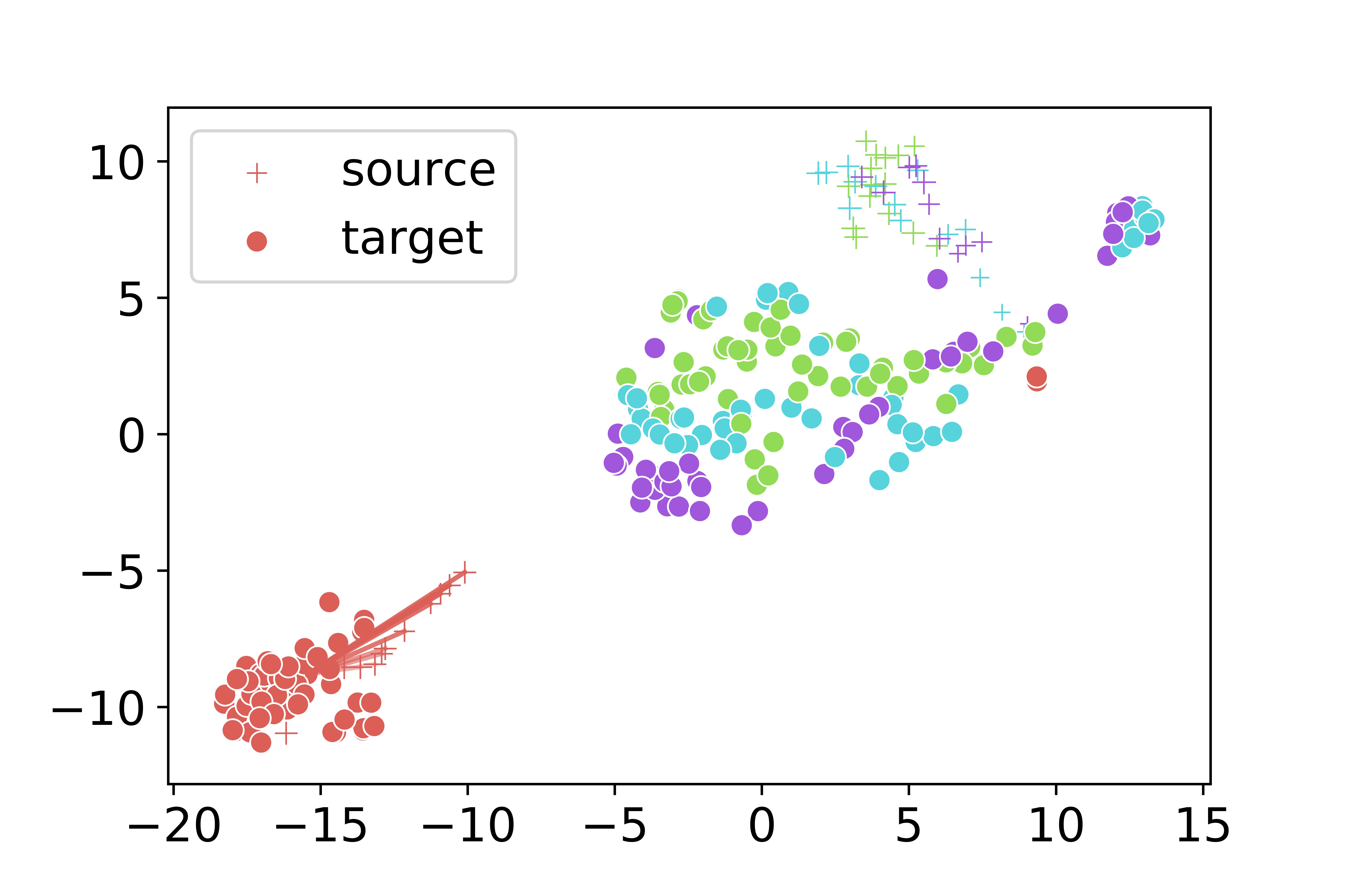
(b) $\eta=0.5$

Figure 8: The group regularizer’s function.

4.5.4 OT-based mapping of substructures

In this part, we illustrate the function of the group regularizer. No group regularizer is used in Figure 8(a) while there is a group regularizer with $\eta=0.5$ is used in Figure 8(b). In Figure 8(a), some points with different colors are linked with the red point while only red points are linked with the red point in Figure 8(b), which are caused by the group regularizer.

4.6 Parameter Sensitivity

In this section, we evaluate the parameter sensitivity of SOT. SOT involves four parameters: $\lambda_{1}$, $\lambda$, $\eta$ and $k_{t}$. We change one parameter and fix the other parameters to observe the performance of SOT. In Figure 9, the red points are the optimal points, and we observe the surrounding results. From 9(a)-9(d), we can see that the results with parameters around the red points are all better than OTDA. The results reveal that SOT is more effective and robust than other methods under different parameters near the optimal.

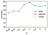
(a) $\lambda_{1}$

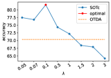
(b) $\lambda$

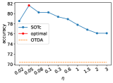
(c) $\eta$

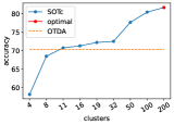
(d) $k_{t}$

Figure 9: Influence of different hyper-parameters.

4.7 Convergence and Time Complexity

In this section, we investigate the convergence and time complexity. In Figure 10(a), we can see SOT convergences in the 10th epoch. And in the actual experiments, 20 epochs are enough for SOT. This means our SOT can reach fast convergence. With the same hyper-parameters, SOT is $\mathbf{5}\times$ faster than traditional OT-based DA methods.

To compare the time complexity, we conduct each experiment 10 times and sum over the time. Figure 10(b) indicates that SOT gets the best accuracy while the time spent is much less than TCA and MLOT. When we slightly change the parameters of OTDA, the time used changes from $71.11$s to $285.32$s. From Figure 10(c), we can see that GMMs use most of the time in SOT. These two parts can be fixed in real experiments, which means we only need to pay attention to the parts of weighting and mapping. Obviously, the time used in the weighting part is negligible, and the time used in the mapping part is smaller than all the other methods compared. In the following, we analyze the time complexity theoretically.

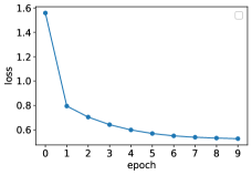
(a) Convergence

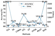
(b) Time Complexity and Accuracy Comparisons

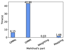
(c) Time Spent of Each Part in SOT

Figure 10: Convergence and Time Complexity.

As we know, without the entropy regularizer, combinatorial algorithms, such as the simplex methods and its network variants, are used to solve the optimal transport. However, their computational complexity is shown to be $O((n_{s}+n_{t})n_{s}n_{t}\log(n_{s}+n_{t}))$, which is impossible to handle large datasets. When handling the OT with the entropy regularizer, we can get an algorithm with the quadratic complexity, which is still below our expectations. The key problem is that $n_{s}$ and $n_{t}$ are too large to get the fast results. To deal with this problem, we use the substructures instead of initial data points. The numbers of the substructures are $k_{s}$ and $k_{t}$ respectively, and they are much smaller than $n_{s}$ and $n_{t}$. To get the substructures, GMM, whose time complexity is $O(L_{1}KN)$, is adopted. $K$ is the number of clusters, $N$ is the number of data, while $L_{1}$ is the number of iterations. We can get the weights of the substructures with one matrix operation and the time spent on this operation is negligible. To sum up, the time complexity of our method is about $O(L_{1}KN+L_{2}K^{2})$, where $L_{1}$ and $L_{2}$ are the numbers of the iterations, and they are much smaller than N.

5 Conclusions and Future Work

Leveraging labeled data from auxiliary domains is a usual way to deal with the label scarcity problem in Human Activity Recognition. In this paper, we propose SSDA to utilize substructures and propose an OT based implementation, SOT, for cross-domain activity recognition. Comparing to existing methods which perform rough matching or sample-level matching, SSDA obtains the internal substructures and completes substructures-level matching which considers more fine-grained locality information of domains and is robust to noise in a certain degree. Comprehensive experiments on four large public datasets demonstrate the significant superiority of SOT over other state-of-the-art methods. In addition, SOT is much faster than other methods, which means it can be used in the larger datasets.

In the future, we plan to extend SOT using deep clustering, as well as applying SSDA to other fine-grained activity recognition problems.

References

- Anguita et al. (2012) Davide Anguita, Alessandro Ghio, Luca Oneto, Xavier Parra, and Jorge L Reyes-Ortiz. Human activity recognition on smartphones using a multiclass hardware-friendly support vector machine. In International workshop on ambient assisted living, pp. 216–223. Springer, 2012.
- Barshan & Yüksek (2014) Billur Barshan and Murat Cihan Yüksek. Recognizing daily and sports activities in two open source machine learning environments using body-worn sensor units. The Computer Journal, 57(11):1649–1667, 2014.
- Beddiar et al. (2020) Djamila Romaissa Beddiar, Brahim Nini, Mohammad Sabokrou, and Abdenour Hadid. Vision-based human activity recognition: a survey. Multimedia Tools and Applications, 79(41):30509–30555, 2020.
- Bhatia et al. (2019) Rajendra Bhatia, Tanvi Jain, and Yongdo Lim. On the bures–wasserstein distance between positive definite matrices. Expositiones Mathematicae, 37(2):165–191, 2019.
- Bux et al. (2017) Allah Bux, Plamen Angelov, and Zulfiqar Habib. Vision based human activity recognition: a review. In Advances in Computational Intelligence Systems, pp. 341–371. Springer, 2017.
- Castro et al. (2016) HF Castro, V Correia, E Sowade, KY Mitra, JG Rocha, RR Baumann, and S Lanceros-Méndez. All-inkjet-printed low-pass filters with adjustable cutoff frequency consisting of resistors, inductors and transistors for sensor applications. Organic Electronics, 38:205–212, 2016.
- Chen & Wang (2018) Zhangjie Chen and Ya Wang. Infrared–ultrasonic sensor fusion for support vector machine–based fall detection. Journal of Intelligent Material Systems and Structures, 29(9):2027–2039, 2018.
- Cook et al. (2013) Diane Cook, Kyle D Feuz, and Narayanan C Krishnan. Transfer learning for activity recognition: A survey. Knowledge and information systems, 36(3):537–556, 2013.
- Courty et al. (2016) Nicolas Courty, Rémi Flamary, Devis Tuia, and Alain Rakotomamonjy. Optimal transport for domain adaptation. IEEE transactions on pattern analysis and machine intelligence, 39(9):1853–1865, 2016.
- Cuturi (2013) Marco Cuturi. Sinkhorn distances: Lightspeed computation of optimal transportation distances. Advances in Neural Information Processing Systems, 26:2292–2300, 2013.
- Dai et al. (2020) Yong Dai, Jian Liu, Xiancong Ren, and Zenglin Xu. Adversarial training based multi-source unsupervised domain adaptation for sentiment analysis. In AAAI, pp. 7618–7625, 2020.
- Dang et al. (2020) L Minh Dang, Kyungbok Min, Hanxiang Wang, Md Jalil Piran, Cheol Hee Lee, and Hyeonjoon Moon. Sensor-based and vision-based human activity recognition: A comprehensive survey. Pattern Recognition, 108:107561, 2020.
- Das & Lee (2018a) Debasmit Das and CS George Lee. Sample-to-sample correspondence for unsupervised domain adaptation. Engineering Applications of Artificial Intelligence, 73:80–91, 2018a.
- Das & Lee (2018b) Debasmit Das and CS George Lee. Unsupervised domain adaptation using regularized hyper-graph matching. In 2018 25th IEEE International Conference on Image Processing (ICIP), pp. 3758–3762. IEEE, 2018b.
- Dawn & Shaikh (2016) Debapratim Das Dawn and Soharab Hossain Shaikh. A comprehensive survey of human action recognition with spatio-temporal interest point (stip) detector. The Visual Computer, 32(3):289–306, 2016.
- Dempster et al. (1977) Arthur P Dempster, Nan M Laird, and Donald B Rubin. Maximum likelihood from incomplete data via the em algorithm. Journal of the Royal Statistical Society: Series B (Methodological), 39(1):1–22, 1977.
- Fernando et al. (2013) Basura Fernando, Amaury Habrard, Marc Sebban, and Tinne Tuytelaars. Unsupervised visual domain adaptation using subspace alignment. In Proceedings of the IEEE international conference on computer vision, pp. 2960–2967, 2013.
- Feuz & Cook (2017) Kyle D Feuz and Diane J Cook. Collegial activity learning between heterogeneous sensors. Knowledge and information systems, 53(2):337–364, 2017.
- Hassan et al. (2018a) Mohammad Mehedi Hassan, Shamsul Huda, Md Zia Uddin, Ahmad Almogren, and Majed Alrubaian. Human activity recognition from body sensor data using deep learning. Journal of medical systems, 42(6):99, 2018a.
- Hassan et al. (2018b) Mohammed Mehedi Hassan, Md Zia Uddin, Amr Mohamed, and Ahmad Almogren. A robust human activity recognition system using smartphone sensors and deep learning. Future Generation Computer Systems, 81:307–313, 2018b.
- Hu et al. (2018) Chunyu Hu, Yiqiang Chen, Lisha Hu, and Xiaohui Peng. A novel random forests based class incremental learning method for activity recognition. Pattern Recognition, 78:277–290, 2018.
- Ignatov (2018) Andrey Ignatov. Real-time human activity recognition from accelerometer data using convolutional neural networks. Applied Soft Computing, 62:915–922, 2018.
- Jia et al. (2020) Guangyu Jia, Hak-Keung Lam, Junkai Liao, and Rong Wang. Classification of electromyographic hand gesture signals using machine learning techniques. Neurocomputing, 2020.
- Kerdoncuff et al. (2020) Tanguy Kerdoncuff, Rémi Emonet, and Marc Sebban. Metric learning in optimal transport for domain adaptation. 2020.
- Khan et al. (2018) Md Abdullah Al Hafiz Khan, Nirmalya Roy, and Archan Misra. Scaling human activity recognition via deep learning-based domain adaptation. In 2018 IEEE International Conference on Pervasive Computing and Communications (PerCom), pp. 1–9. IEEE, 2018.
- Khan & Taati (2017) Shehroz S Khan and Babak Taati. Detecting unseen falls from wearable devices using channel-wise ensemble of autoencoders. Expert Systems with Applications, 87:280–290, 2017.
- Li et al. (2020) Juntao Li, Ruidan He, Hai Ye, Hwee Tou Ng, Lidong Bing, and Rui Yan. Unsupervised domain adaptation of a pretrained cross-lingual language model. arXiv preprint arXiv:2011.11499, 2020.
- Lin et al. (2016) Yuewei Lin, Jing Chen, Yu Cao, Youjie Zhou, Lingfeng Zhang, Yuan Yan Tang, and Song Wang. Cross-domain recognition by identifying joint subspaces of source domain and target domain. IEEE transactions on cybernetics, 47(4):1090–1101, 2016.
- Long et al. (2013) Mingsheng Long, Jianmin Wang, Guiguang Ding, Jiaguang Sun, and Philip S Yu. Transfer feature learning with joint distribution adaptation. In Proceedings of the IEEE international conference on computer vision, pp. 2200–2207, 2013.
- Pan & Yang (2009) Sinno Jialin Pan and Qiang Yang. A survey on transfer learning. IEEE Transactions on knowledge and data engineering, 22(10):1345–1359, 2009.
- Pan et al. (2010) Sinno Jialin Pan, Ivor W Tsang, James T Kwok, and Qiang Yang. Domain adaptation via transfer component analysis. IEEE Transactions on Neural Networks, 22(2):199–210, 2010.
- Peyré et al. (2019) Gabriel Peyré, Marco Cuturi, et al. Computational optimal transport: With applications to data science. Foundations and Trends® in Machine Learning, 11(5-6):355–607, 2019.
- Qin et al. (2019) Xin Qin, Yiqiang Chen, Jindong Wang, and Chaohui Yu. Cross-dataset activity recognition via adaptive spatial-temporal transfer learning. Proceedings of the ACM on Interactive, Mobile, Wearable and Ubiquitous Technologies, 3(4):1–25, 2019.
- Redko et al. (2017) Ievgen Redko, Amaury Habrard, and Marc Sebban. Theoretical analysis of domain adaptation with optimal transport. In Joint European Conference on Machine Learning and Knowledge Discovery in Databases, pp. 737–753. Springer, 2017.
- Reiss & Stricker (2012) Attila Reiss and Didier Stricker. Introducing a new benchmarked dataset for activity monitoring. In 2012 16th International Symposium on Wearable Computers, pp. 108–109. IEEE, 2012.
- Rey & Lukowicz (2017) Vitor F Rey and Paul Lukowicz. Label propagation: An unsupervised similarity based method for integrating new sensors in activity recognition systems. Proceedings of the ACM on Interactive, Mobile, Wearable and Ubiquitous Technologies, 1(3):1–24, 2017.
- Reyes-Ortiz et al. (2016) Jorge-L Reyes-Ortiz, Luca Oneto, Albert Samà, Xavier Parra, and Davide Anguita. Transition-aware human activity recognition using smartphones. Neurocomputing, 171:754–767, 2016.
- Rokni & Ghasemzadeh (2018) Seyed Ali Rokni and Hassan Ghasemzadeh. Autonomous training of activity recognition algorithms in mobile sensors: A transfer learning approach in context-invariant views. IEEE Transactions on Mobile Computing, 17(8):1764–1777, 2018.
- Schwarz et al. (1978) Gideon Schwarz et al. Estimating the dimension of a model. The annals of statistics, 6(2):461–464, 1978.
- Sun et al. (2016) Baochen Sun, Jiashi Feng, and Kate Saenko. Return of frustratingly easy domain adaptation. In AAAI Conference on Artificial Intelligence (AAAI), 2016.
- Tan et al. (2018) Chuanqi Tan, Fuchun Sun, Tao Kong, Wenchang Zhang, Chao Yang, and Chunfang Liu. A survey on deep transfer learning. In International conference on artificial neural networks, pp. 270–279. Springer, 2018.
- Triboan et al. (2019) Darpan Triboan, Liming Chen, Feng Chen, and Zumin Wang. A semantics-based approach to sensor data segmentation in real-time activity recognition. Future Generation Computer Systems, 93:224–236, 2019.
- Villani (2008) Cédric Villani. Optimal transport: old and new, volume 338. Springer Science & Business Media, 2008.
- Wang et al. (2017) Jindong Wang, Yiqiang Chen, Shuji Hao, Wenjie Feng, and Zhiqi Shen. Balanced distribution adaptation for transfer learning. In 2017 IEEE International Conference on Data Mining (ICDM), pp. 1129–1134. IEEE, 2017.
- Wang et al. (2018a) Jindong Wang, Yiqiang Chen, Lisha Hu, Xiaohui Peng, and S Yu Philip. Stratified transfer learning for cross-domain activity recognition. In 2018 IEEE International Conference on Pervasive Computing and Communications (PerCom), pp. 1–10. IEEE, 2018a.
- Wang et al. (2018b) Jindong Wang, Wenjie Feng, Yiqiang Chen, Han Yu, Meiyu Huang, and Philip S Yu. Visual domain adaptation with manifold embedded distribution alignment. In Proceedings of the 26th ACM international conference on Multimedia, pp. 402–410, 2018b.
- Wang et al. (2019) Jindong Wang, Yiqiang Chen, Shuji Hao, Xiaohui Peng, and Lisha Hu. Deep learning for sensor-based activity recognition: A survey. Pattern Recognition Letters, 119:3–11, 2019.
- Wang et al. (2020) Jindong Wang, Yiqiang Chen, Wenjie Feng, Han Yu, Meiyu Huang, and Qiang Yang. Transfer learning with dynamic distribution adaptation. ACM Transactions on Intelligent Systems and Technology (TIST), 11(1):1–25, 2020.
- (49) Jindong Wang et al. Everything about transfer learning and domain adapation. http://transferlearning.xyz.
- Wang & Deng (2018) Mei Wang and Weihong Deng. Deep visual domain adaptation: A survey. Neurocomputing, 312:135–153, 2018.
- Weinberger & Saul (2009) Kilian Q Weinberger and Lawrence K Saul. Distance metric learning for large margin nearest neighbor classification. Journal of Machine Learning Research, 10(2), 2009.
- Weiss et al. (2016) Karl Weiss, Taghi M Khoshgoftaar, and DingDing Wang. A survey of transfer learning. Journal of Big data, 3(1):9, 2016.
- Wilson & Cook (2020) Garrett Wilson and Diane J Cook. A survey of unsupervised deep domain adaptation. ACM Transactions on Intelligent Systems and Technology (TIST), 11(5):1–46, 2020.
- Xiao & Song (2018) Qinkun Xiao and Ren Song. Action recognition based on hierarchical dynamic bayesian network. Multimedia Tools and Applications, 77(6):6955–6968, 2018.
- Zhang & Sawchuk (2012) Mi Zhang and Alexander A. Sawchuk. Usc-had: A daily activity dataset for ubiquitous activity recognition using wearable sensors. In ACM International Conference on Ubiquitous Computing (Ubicomp) Workshop on Situation, Activity and Goal Awareness (SAGAware), Pittsburgh, Pennsylvania, USA, September 2012.
- Zhao et al. (2018a) Aite Zhao, Lin Qi, Jie Li, Junyu Dong, and Hui Yu. A hybrid spatio-temporal model for detection and severity rating of parkinson’s disease from gait data. Neurocomputing, 315:1–8, 2018a.
- Zhao et al. (2020) Jiachen Zhao, Fang Deng, Haibo He, and Jie Chen. Local domain adaptation for cross-domain activity recognition. IEEE Transactions on Human-Machine Systems, 2020.
- Zhao et al. (2017) Mingmin Zhao, Shichao Yue, Dina Katabi, Tommi S Jaakkola, and Matt T Bianchi. Learning sleep stages from radio signals: A conditional adversarial architecture. In International Conference on Machine Learning, pp. 4100–4109, 2017.
- Zhao et al. (2018b) Yu Zhao, Rennong Yang, Guillaume Chevalier, Ximeng Xu, and Zhenxing Zhang. Deep residual bidir-lstm for human activity recognition using wearable sensors. Mathematical Problems in Engineering, 2018, 2018b.
- Zhao et al. (2011) Zhongtang Zhao, Yiqiang Chen, Junfa Liu, Zhiqi Shen, and Mingjie Liu. Cross-people mobile-phone based activity recognition. In Twenty-second international joint conference on artificial intelligence, 2011.
- Zhu et al. (2020) Yongchun Zhu, Fuzhen Zhuang, Jindong Wang, Guolin Ke, Jingwu Chen, Jiang Bian, Hui Xiong, and Qing He. Deep subdomain adaptation network for image classification. IEEE Transactions on Neural Networks and Learning Systems, 2020.